Article

Time-Series MODIS-Based Remote Sensing and Explainable Machine Learning for Assessing Grassland Resilience in Arid Regions

1
State Key Laboratory of Ecological Safety and Sustainable Development in Arid Lands, Xinjiang Institute of Ecology and Geography, Chinese Academy of Sciences, Urumqi 830011, China
2
University of Chinese Academy of Sciences, Beijing 100049, China
3
Polish-Chinese Centre for Environmental Research, Institute of Earth Sciences, University of Silesia in Katowice, 40-007 Katowice, Poland
*
Author to whom correspondence should be addressed.
Remote Sens. 2025, 17(16), 2749; https://doi.org/10.3390/rs17162749
Submission received: 13 June 2025 / Revised: 3 August 2025 / Accepted: 4 August 2025 / Published: 8 August 2025

Abstract

Grassland ecosystems in arid regions increasingly experience resilience loss due to intensifying climatic variability. However, the limited interpretability of conventional machine learning models constrains our understanding of underlying ecological drivers. This study constructs an integrative framework that combines temporal autocorrelation (TAC) metrics with explainable machine learning, employing Random Forest and SHAP (SHapley Additive exPlanations) analysis. Time series of satellite-derived vegetation indices from MODIS (2001–2023), particularly the kernel Normalized Difference Vegetation Index (KNDVI), support the generation of TAC and its trend-based derivative δTAC. The framework assesses ecosystem resilience across seven representative grassland types in Xinjiang, capturing diverse responses to climate variability and vegetation dynamics. Results reveal pronounced spatial heterogeneity: resilience declines in radiation-stressed arid zones, while hydrothermally stable regions maintain stronger recovery capacity. Key drivers include temperature variability and vegetation dynamics, with divergent effects among grassland types. Meadow and Typical Steppe exhibit higher resilience under stable hydrothermal regimes, whereas desert and alpine systems show greater sensitivity to warming and climatic fluctuations. This framework enhances diagnostic transparency and ecological insight, offering a spatially explicit, data-driven tool for resilience monitoring. The findings support the formulation of targeted adaptation strategies and sustainable grassland management in response to ongoing climate change.

1. Introduction

Grassland ecosystems cover approximately 30–40% of Earth’s terrestrial surface, support biodiversity, regulate climate, and drive global biogeochemical cycles [1,2,3]. These systems have underpinned rural livelihoods, particularly in arid and semi-arid regions, where ecological functions directly sustain socio-economic stability [4,5]. In recent decades, intensifying climate variability and anthropogenic disturbances have accelerated grassland degradation, with nearly half of global rangelands now affected [6,7] Compound stressors—such as droughts, heatwaves, and altered precipitation regimes—have continued to impair ecosystem functioning [8,9,10]. Although grasslands play essential roles in sustaining ecological and economic systems, most existing studies have emphasized static indicators such as biomass, productivity, or carbon storage [11,12,13]. These indicators reflect the ecosystem state but fail to capture the capacity to recover after disturbance—an essential component of long-term stability [14,15]. This gap persists despite growing recognition of resilience as a critical dimension of ecosystem response [14,16,17]. Accurately evaluating resilience presents a major challenge, especially with increasing climate and human impacts [18].
Efforts to quantify resilience have often relied on empirical indices or linear statistical models, which fail to account for the complexity and nonlinearity inherent in dryland ecosystems [19]. In contrast, machine learning (ML) methods can accommodate high-dimensional interactions and nonlinear responses, offering a flexible modeling framework for ecological inference [20,21,22]. However, limited interpretability has constrained the practical utility of conventional ML models. Explainable machine learning (XML) techniques bridge this gap by integrating predictive accuracy with model transparency [23,24,25]. Random Forest (RF), a robust tree-based ensemble learning algorithm, enables nonlinear modeling across heterogeneous landscapes. SHapley Additive exPlanations (SHAP), grounded in cooperative game theory, can disaggregate model outputs to quantify the marginal effect of each predictor [26]. Recent studies have applied SHAP to forest productivity, species distribution, and ecosystem state transition [27,28,29]. However, few have extended these tools to resilience assessment in grassland ecosystems.
Resilience, first introduced by Holling (1973) [30], refers to an ecosystem’s ability to absorb disturbances while maintaining essential functions and structure. Later distinctions identified engineering resilience—rapid return to equilibrium—and ecological resilience, which emphasizes persistence and adaptive capacity [31,32]. Among quantitative indicators, temporal autocorrelation (TAC) emerged as a robust proxy for assessing ecological resilience, particularly through remotely sensed vegetation indices. TAC quantifies system memory and recovery lag by measuring the correlation of an ecosystem state variable with its previous value, typically at a one-year lag (AC1) [19]. This approach does not rely on disturbance annotations and has been successfully applied across various ecosystems including forests, wetlands, and grasslands [19,33,34]. The advantages of TAC lie in its ability to detect critical slowing down and provide early warning signals of regime shifts under increasing environmental pressure. Its consistent performance across spatial and temporal scales makes it particularly suitable for long-term resilience monitoring using remote sensing data. In this study, TAC was derived from an AC1 of standardized anomalies in KNDVI, a widely used proxy for vegetation dynamics and ecosystem state. Lower TAC values indicate faster post-disturbance recovery and thus greater resilience. KNDVI has been extensively adopted in resilience-related studies due to its sensitivity to vegetation changes and compatibility with high-temporal-resolution remote sensing products [35,36,37,38]. It also supports the detection of spatial vegetation heterogeneity and landscape-scale responses to climate-induced disturbances when integrated with spatial simulation methods [39]. By applying this framework across multiple grassland types, the objective was to reveal spatial patterns and the principal climatic and ecological factors influencing resilience variability.
Northwest China, particularly the Xinjiang region, encompasses a broad spectrum of ecological conditions shaped by diverse topography, steep climatic gradients, and over 50 million hectares of grassland. These grasslands range from alpine meadows in the Altai Mountains—characterized by cold and humid high-altitude environments—to desert–steppe mosaics around the Tarim Basin, dominated by strong solar radiation and moisture deficits [40,41,42]. These grassland formations reflect the interplay of natural zonation, edaphic conditions, and long-term land use history, including traditional grazing practices. Human disturbances such as overgrazing, land reclamation, and infrastructure development further modulate ecological processes, intensifying vegetation stress and altering resilience patterns. As such, Xinjiang provides a heterogeneous and representative landscape for examining how different grassland ecosystems respond to multifactor stressors. However, limited research has applied TAC-based metrics in this context, and few studies have integrated explainable machine learning approaches to investigate how specific climatic factors influence resilience trajectories across different grassland types.
This study constructs a spatiotemporal framework for assessing grassland resilience across Xinjiang from 2001 to 2023. The analysis integrates TAC and δTAC with RF modeling and SHAP-based interpretation. Specifically, we carried out the following work: (1) developing a resilience modeling structure using vegetation indicators and climatic factors; (2) quantifying resilience magnitude and trends through TAC and δTAC; (3) interpreting the relative influence of environmental drivers using SHAP. This approach enhances ecological insight into resilience dynamics, supports early diagnosis of degradation risks, and informs adaptive management strategies in dryland systems increasingly exposed to climatic instability.

2. Materials and Methods

2.1. Study Area

The Xinjiang Uygur Autonomous Region in Northwest China spans approximately 1.66 million km2, accounting for one-sixth of the country’s land area (Figure 1). The region features significant topographic variation, with mountain ranges like the Altai, Tianshan, and Kunlun–Karakoram separating the Junggar and Tarim Basins. Elevation ranges from −157 m to 8566 m, contributing to pronounced ecological and climatic differences.
A strongly continental arid climate dominates Xinjiang, with precipitation generally low but highly variable due to complex terrain. Annual precipitation ranges from less than 50 mm in hyper-arid basins like Turpan and Hotan to over 450 mm in mountainous areas such as Ili and Altai. On average, the region receives around 200 mm of rainfall per year, while potential evaporation exceeds 4500 mm, and annual sunshine duration can reach 3600 h. These extreme hydrothermal conditions constrain vegetation growth and contribute to ecological fragility across the region. Land cover data derived from the 2020 China Land Cover Dataset (CLCD) indicate that unused land dominates (62.3%) in Xinjiang, followed by grassland (24.1%) mainly distributed along the Tianshan and Altai foothills, cropland (6.8%) in the Ili River Valley and southern oasis zones, forest (3.5%) at high altitudes, and limited built-up (1.2%) and water areas (2.1%). As China’s second-largest pastoral region, Xinjiang supports ~52 million hectares of grassland—about 20% of the national total—playing a critical role in biodiversity conservation, ecological regulation, and rural livelihoods [44,45].
Seven major grassland types reflect Xinjiang’s ecological heterogeneity: Temperate Meadow Steppe, Temperate Typical Steppe, Temperate Desert Steppe, Temperate Steppe Desert, Temperate Desert, Alpine Steppe, and Other Vegetation. These types span a gradient from humid and thermally moderate conditions in the north and northwest to increasingly arid, high-radiation environments in the south and interior. Temperate Meadow Steppe occurs under optimal hydrothermal conditions, with the highest productivity and vegetation indices. Typical Steppe forms in moderately warm and moist regions, supporting stable vegetation and intermediate productivity. Transitional types—Temperate Desert Steppe and Steppe Desert—develop under drier, warmer conditions and exhibit more variable vegetation responses. The Temperate Desert, shaped by intense radiation and limited rainfall, hosts sparse, drought-adapted plant communities. Alpine Steppe, distributed at high elevations, experiences severe thermal limitations but maintains moderate-to-high KNDVI and FVC values during its brief growing season.
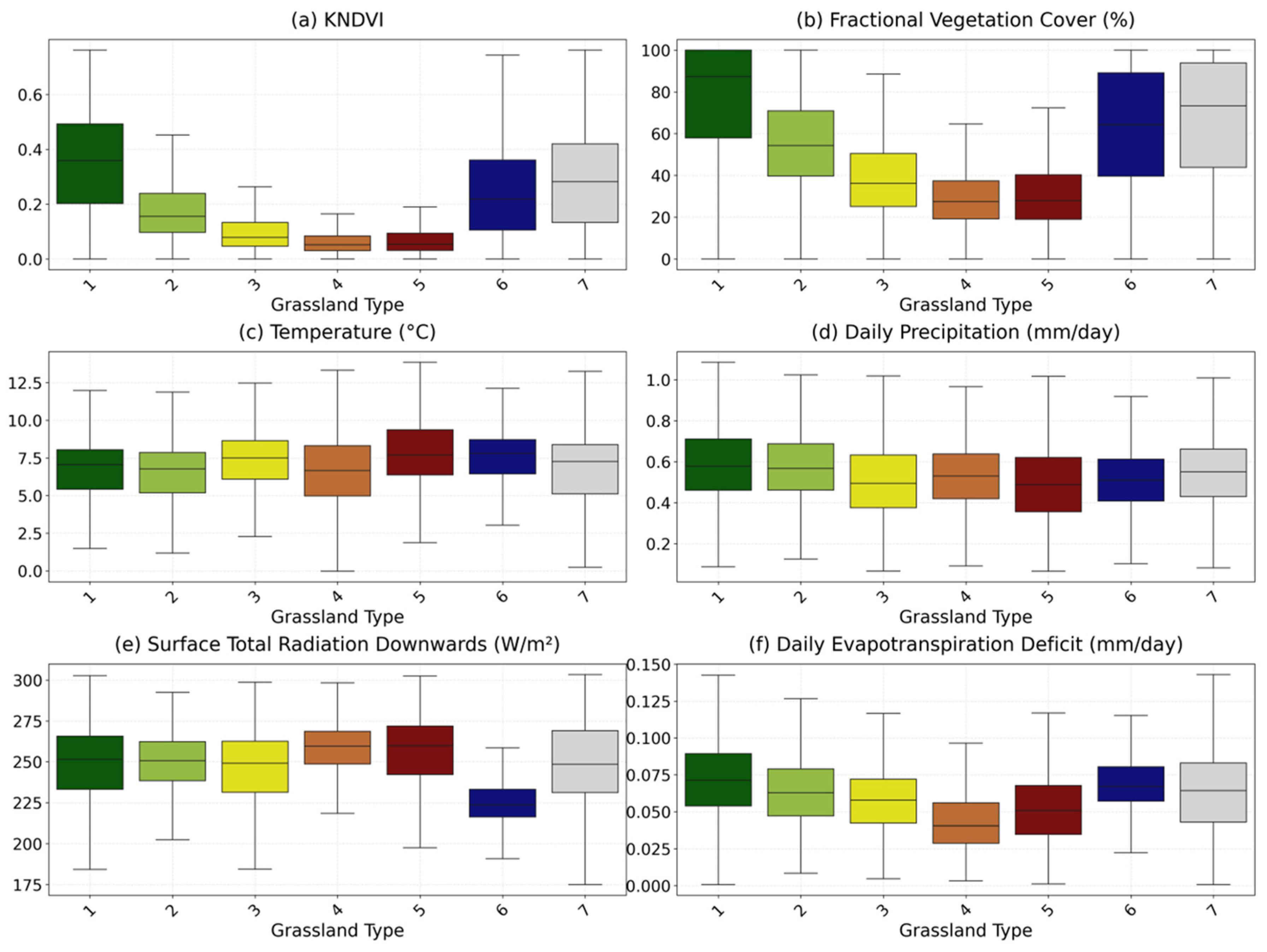
Environmental variables exhibit clear gradients across these types (Figure 2): mean temperature peaks in desert and transitional types, while Alpine Steppe records the lowest temperatures. Precipitation is highest in Temperate Meadow Steppe and declines toward arid systems. Notably, Alpine Steppe receives precipitation levels similar to some desert systems, indicating that temperature—not moisture—is the dominant limiting factor in high-altitude ecosystems. Surface total radiation (STRD) increases modestly with aridity, while evapotranspiration deficit (ETD) shows more complex patterns, shaped by both atmospheric demand and vegetation structure. These climate–vegetation gradients highlight the ecological distinctiveness of each grassland type. Variations in vegetation cover, climatic sensitivity, and hydrothermal constraints suggest that different grassland types exhibit distinct resilience patterns and responses to external stressors such as drought, warming, or radiation pressure. Consequently, resilience assessment must be type-specific, reflecting both the local environment and the intrinsic ecological traits of each grassland system.

2.2. Dataset

This study used multiple gridded and station-based datasets to characterize climate, vegetation, and land use patterns in Xinjiang from 2000 to 2023. The data sources and descriptions are summarized in Table 1.
Daily precipitation and temperature records (2001–2019) were obtained from the China Surface Climate Daily Dataset (V3.0) provided by the China Meteorological Administration (http://data.cma.cn/, accessed on 11 August 2024). Data for 2020–2023 were estimated using linear regression based on national-level observations [46,47].
Surface total radiation downward (STRD) and evapotranspiration (ET) (2001–2023) were obtained from the ERA5 hourly reanalysis dataset (https://cds.climate.copernicus.eu, accessed on 3 September 2024). These data have a native spatial resolution of approximately 0.25° (25 km) [48].
Normalized Difference Vegetation Index (NDVI) data were obtained from the MODIS MOD13A2 Version 6 product [49] (https://lpdaac.usgs.gov/products/mod13a2v006/, accessed on 6 August 2024), which provides 16-day composites at 1 km spatial resolution.
Fractional Vegetation Cover (FVC) data were obtained from a 250 m resolution dataset published by Gao Jixi et al. (2024) [50] through the National Tibetan Plateau Data Center (https://data.tpdc.ac.cn, accessed on 19 October 2024).
Land use data (2000–2023) were sourced from Wuhan University’s State Key Laboratory of Surveying and Mapping Remote Sensing (https://zenodo.org/records/12779975, accessed on 20 July 2024). The original resolution of this dataset is 30 m [43].
Grassland ecosystem types were obtained from a 1 km classification dataset published by Tang et al. (2020) [51] based on the national vegetation map of China (https://data.tpdc.ac.cn/zh-hans/data/20722773-9955-4d6e-a761-ed23814aca41, accessed on 14 December 2024).

2.3. Methodology

All data processing and analysis were conducted using ArcGIS 10.8 and Python 3.9. This study established an integrated framework to assess grassland resilience across Xinjiang from 2001 to 2023. Vegetation resilience was characterized by TAC of vegetation indices, which reflects the system’s recovery ability after climate disturbances. Key variables include vegetation metrics (KNDVI and FVC), temperature, precipitation, surface radiation, and evapotranspiration deficit. A Random Forest (RF) model was used to explore the relationship between TAC and environmental drivers. To enhance interpretability, the SHAP method was applied to quantify the relative importance of each predictor and provide transparent insights into resilience mechanisms.

2.3.1. Data Preprocessing

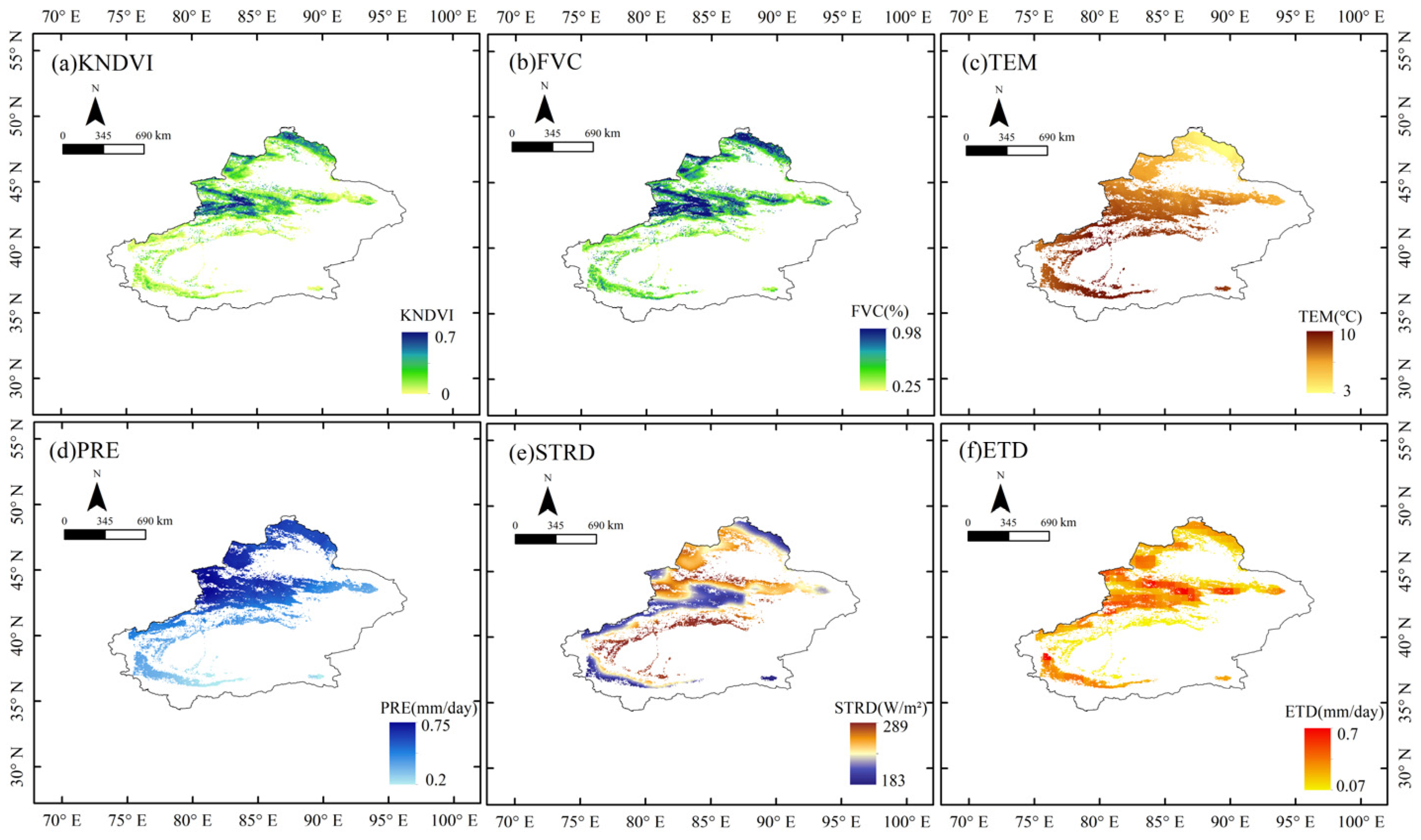
Land use data were first resampled from 30 m to 1 km resolution using the Resample tool in ArcGIS 10.8, and only pixels classified as grassland were retained. These pixels were then converted to point data, with coordinates rounded to five decimal places to generate a fixed spatial reference grid. Grassland type classification data were overlaid on this grid, and only types 1 to 7 were selected for further analysis. Daily precipitation and temperature records from 54 meteorological stations were averaged annually and spatialized using Kriging interpolation to produce continuous raster surfaces. ERA5 hourly data, including surface radiation and evapotranspiration, were first aggregated to annual means and then interpolated to the reference points using cubic interpolation based on georeferenced raster layers. Raster values from all datasets were extracted to the unified point grid using the Extract Values to Points tool with the INTERPOLATE option enabled. NDVI and FVC data were aggregated to annual means prior to extraction. Missing values in the resulting panel dataset were filled using a five-nearest-neighbor interpolation. After all filtering steps, a total of 290,010 annual grassland observations were retained from 2001 to 2023. For each climatic variable, the coefficient of variation was calculated over a two-year moving window to represent short-term variability, while one-year-lagged autocorrelation was computed to indicate temporal persistence. The spatial distributions of the six primary predictor variables—KNDVI, FVC, TEM, PRE, STRD, and ETD—are provided in Figure 3 to support the preprocessing and modeling processes.

2.3.2. Random Forest Model for Long-Term TAC

An RF regression model assessed drivers of long-term TAC, used here as a proxy for ecological resilience. TAC was computed using standardized anomalies of KNDVI with a one-year lag:
T A C ( τ ) = C o v ( X t , X ( t τ ) ) V a r ( X t )
where X t denotes the standardized anomaly of KNDVI in year t. Input variables included vegetation indicators (KNDVI, FVC), climatic means (PRE, TEM, STRD, ETD), variability metrics (CVs over two-year windows), and autocorrelations (ACs based on one-year lags). The RF model used 80% of the data for training and 20% for testing, with 100 trees. Model performance was evaluated using the coefficient of determination (R2) and root mean square error (RMSE), defined, respectively, as
R 2 = 1 i = 1 n ( y i y i ^ ) 2 i = 1 n ( y i y ¯ ) 2
RMSE = 1 n i = 1 n ( y i y i ^ ) 2
where y i is the observed value, y i ^ is the predicted value, y ¯ is the mean of observed values, and n is the number of samples. R2 measures the proportion of variance in the observed data explained by the model, with values closer to 1 indicating better fit. RMSE quantifies the average prediction error in the same units as the target variable, with lower values indicating higher accuracy. A complete list of environmental variables used in the RF model, along with their categories and abbreviations, is provided in Table 2.

2.3.3. Calculation of Enhanced TAC and Linear Trend (δTAC)

Annual TAC values were predicted using RF models and recalculated with fixed lag-1 AC values from 2001. This isolated the portion of TAC attributable to climate autocorrelation:
T A C a c = T A C 1 T A C 2
where T A C 1 represents the annual TAC derived from the original RF model and T A C 2 is the TAC predicted using the fixed autocorrelation values from 2001. The Enhanced TAC was calculated as the difference between these two:
T A C e n h a n c e d = T A C t T A C a c
where T A C t denotes the annual TAC and T A C a c reflects the autocorrelation-derived portion. The trend of Enhanced TAC was quantified using the slope of the regression line over time:
δ T A C = t = 1 n ( t t ¯ ) ( T A C ( e n h a n c e d , t ) T A C e n h a n c e d ¯ ) t = 1 n ( t t ¯ ) 2
Negative TAC indicates resilience gain, while positive values indicate resilience loss.

2.3.4. SHAP-Driven Explainability Analysis

SHAP is an interpretable machine learning method based on cooperative game theory. It calculates the contribution of each feature to a model prediction by simulating all possible combinations of features and evaluating how much each feature adds when it is included. The Shapley value for a feature is the average of its marginal contributions across all possible feature subsets. This method ensures a fair and consistent allocation of contribution scores, satisfying properties such as additivity and symmetry.
ϕ i = S F \ i | S | ! ( | F | | S | 1 ) ! | F | ! f ( S i f ( S )
where ϕ i denotes the SHAP value assigned to feature i , F represents the complete set of features, S F \ i is any subset not containing feature i , and f ( S ) refers to the model prediction based only on the subset S .
Unlike traditional feature importance methods in machine learning—such as the mean decrease in impurity in Random Forest—SHAP provides local interpretability by assigning a separate contribution value to each feature for each individual prediction. It also accounts for feature interactions and avoids bias toward features with many categories or high variance. This makes SHAP particularly suited for understanding complex ecological processes with nonlinear interactions.
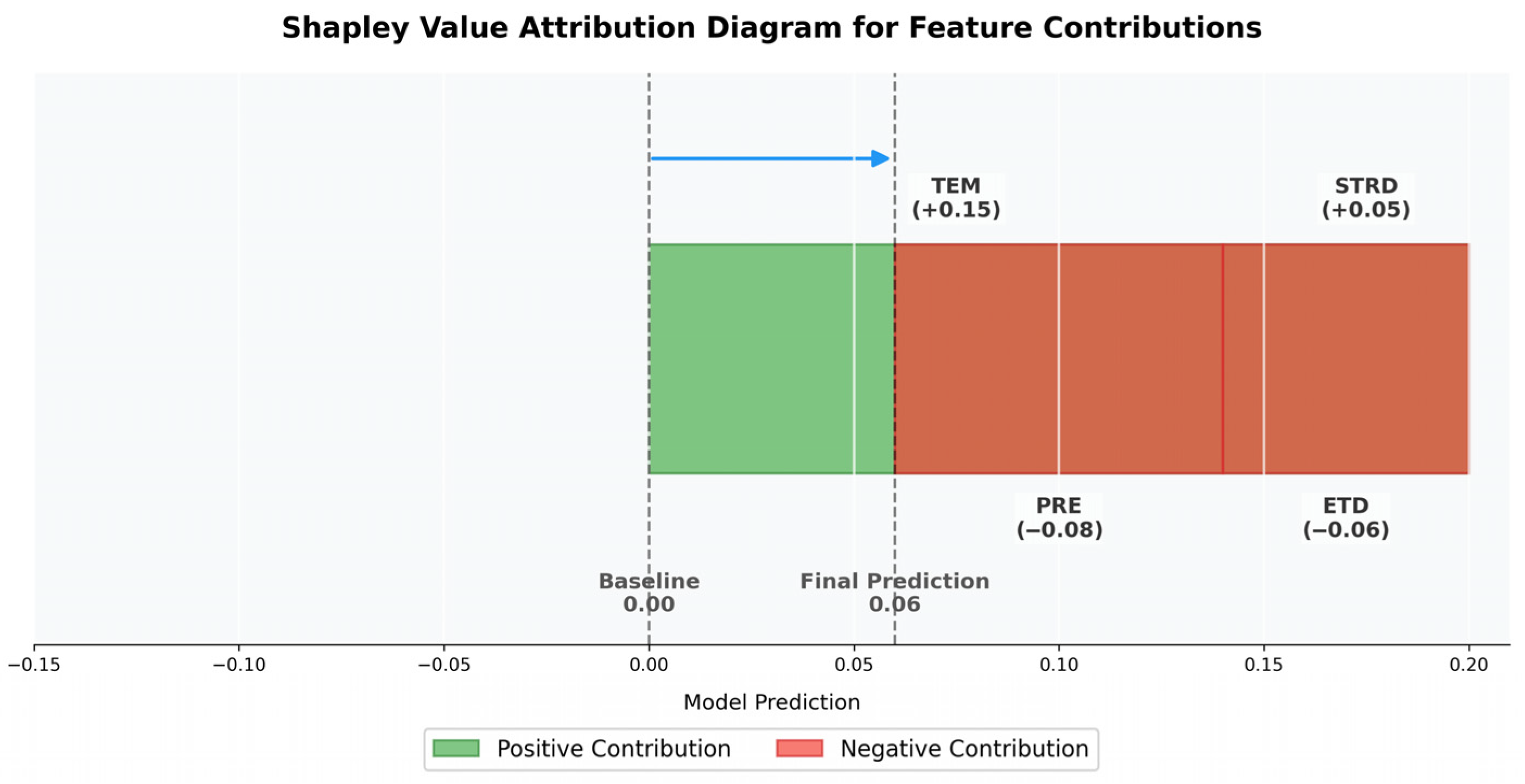
Figure 4 further details the attribution of Shapley values to the individual features in relation to the final model prediction. This plot illustrates how each predictor variable influences a single prediction of the Random Forest model for δTAC. The baseline (0.00) represents the centered SHAP value, corresponding to the model’s average prediction across all samples. The final prediction (+0.06) indicates that this sample’s output is 0.06 units above the mean model prediction. TEM contributes positively (+0.15), pushing the prediction upward; PRE and ETD both contribute negatively (−0.08 and −0.06, respectively), lowering the prediction; STRD has a small positive contribution (+0.05). The green bars represent positive contributions to the model output, while the red bars represent negative effects. This example highlights how SHAP values help disentangle the role of each feature in localized prediction outcomes, aiding model interpretability.

3. Results

3.1. Spatiotemporal Patterns of Grassland Resilience

3.1.1. Spatiotemporal Distribution of Long-Term TAC

TAC serves as a quantitative proxy for ecosystem resilience, capturing the degree to which vegetation conditions each year depend on the previous year’s state. Higher TAC values reflect stronger system inertia and slower recovery from perturbations, indicating reduced resilience. In contrast, lower TAC values signal rapid recovery and high adaptive capacity.
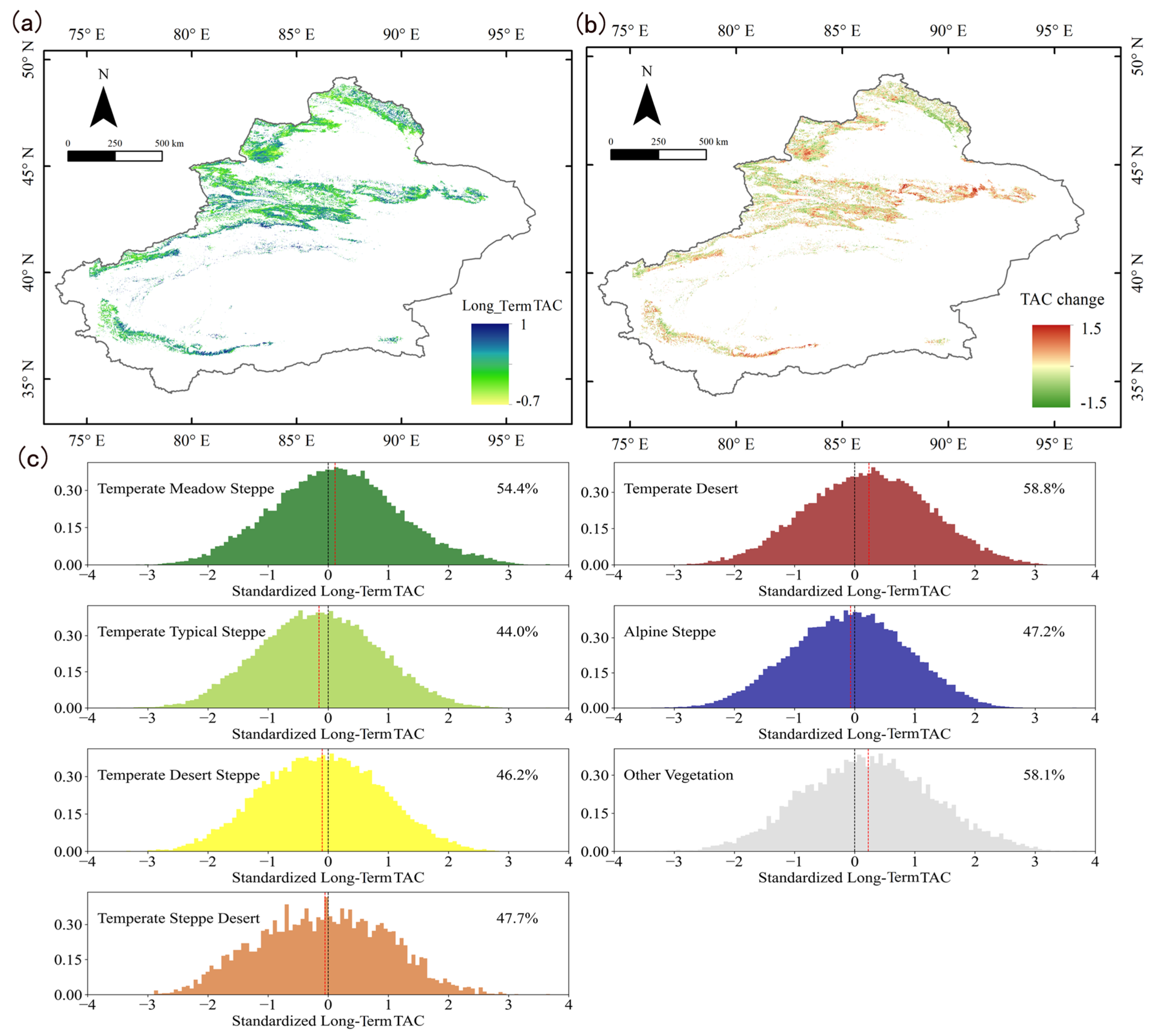
Long-term TAC, calculated from standardized KNDVI anomalies over the 2001–2023 period, revealed distinct spatial gradients in resilience across Xinjiang (Figure 5a). Lower TAC values dominated the northern, northwestern, and central regions, indicating high resilience under favorable hydrothermal conditions and relatively stable disturbance regimes. These areas typically corresponded to Temperate Meadow Steppe and Temperate Typical Steppe zones, where precipitation and thermal stability supported rapid vegetative recovery. In contrast, higher TAC values appeared prominently in the southern and southeastern portions of the study area, particularly within Temperate Desert and Steppe Desert grasslands. These regions experience persistent aridity, intense solar radiation, and limited vegetative buffering capacity, which collectively reduce recovery rates and increase system inertia—manifesting as diminished resilience.
Temporal comparisons between the early (2001–2010) and recent (2011–2023) periods (Figure 5b) highlighted that 39% of grassland areas showed increasing TAC values over time, indicating resilience decline. These changes are most evident in arid grasslands and ecotonal regions, suggesting the influence of intensified climatic stress, prolonged drought episodes, and cumulative ecosystem degradation. Conversely, declining TAC trends in the north and northwest implied enhanced resilience, possibly linked to ecological restoration, reduced disturbance, or favorable climatic shifts.
Standardized TAC distributions further differentiated resilience characteristics across grassland types (Figure 5c). Temperate Desert and Other Vegetation exhibited right-skewed distributions, with a concentration of high TAC values indicative of weak resilience. In contrast, Temperate Typical Steppe, Desert Steppe, Steppe Desert, and Alpine Steppe showed more symmetric distributions centered around lower TAC values, reflecting higher overall resilience and stronger recovery capacity under disturbance.
These spatiotemporal patterns highlight that grassland resilience in Xinjiang is governed by both large-scale environmental gradients and the functional characteristics of different grassland types, underscoring the need for integrated assessments that reflect long-term ecological variability and system heterogeneity.

3.1.2. Spatiotemporal Distribution of Enhanced TAC and δTAC

Enhanced TAC was calculated by recalculating annual TAC using fixed lag-1 autocorrelation values from 2001, thereby isolating and removing the influence of climate memory. This adjustment allows clearer attribution of resilience to vegetation dynamics rather than persistent climatic effects. While long-term TAC reflects overall resilience by capturing vegetation recovery delays, it is sensitive to serial climate variability such as sustained drought or warming. Enhanced TAC removes this confounding factor and highlights the intrinsic capacity of ecosystems to recover after disturbance, independent of low-frequency climatic persistence.
δTAC, defined as the temporal slope of Enhanced TAC, quantifies the direction and magnitude of resilience change. Unlike TAC, which represents average system inertia, δTAC captures resilience trends—whether systems are becoming more stable or increasingly fragile over time. Together, long-term TAC, Enhanced TAC, and δTAC offer complementary insights: the first reflects integrated recovery behavior under full climatic influence, the second reveals the vegetation system’s own recovery characteristics, and the third tracks long-term changes in resilience trajectory.
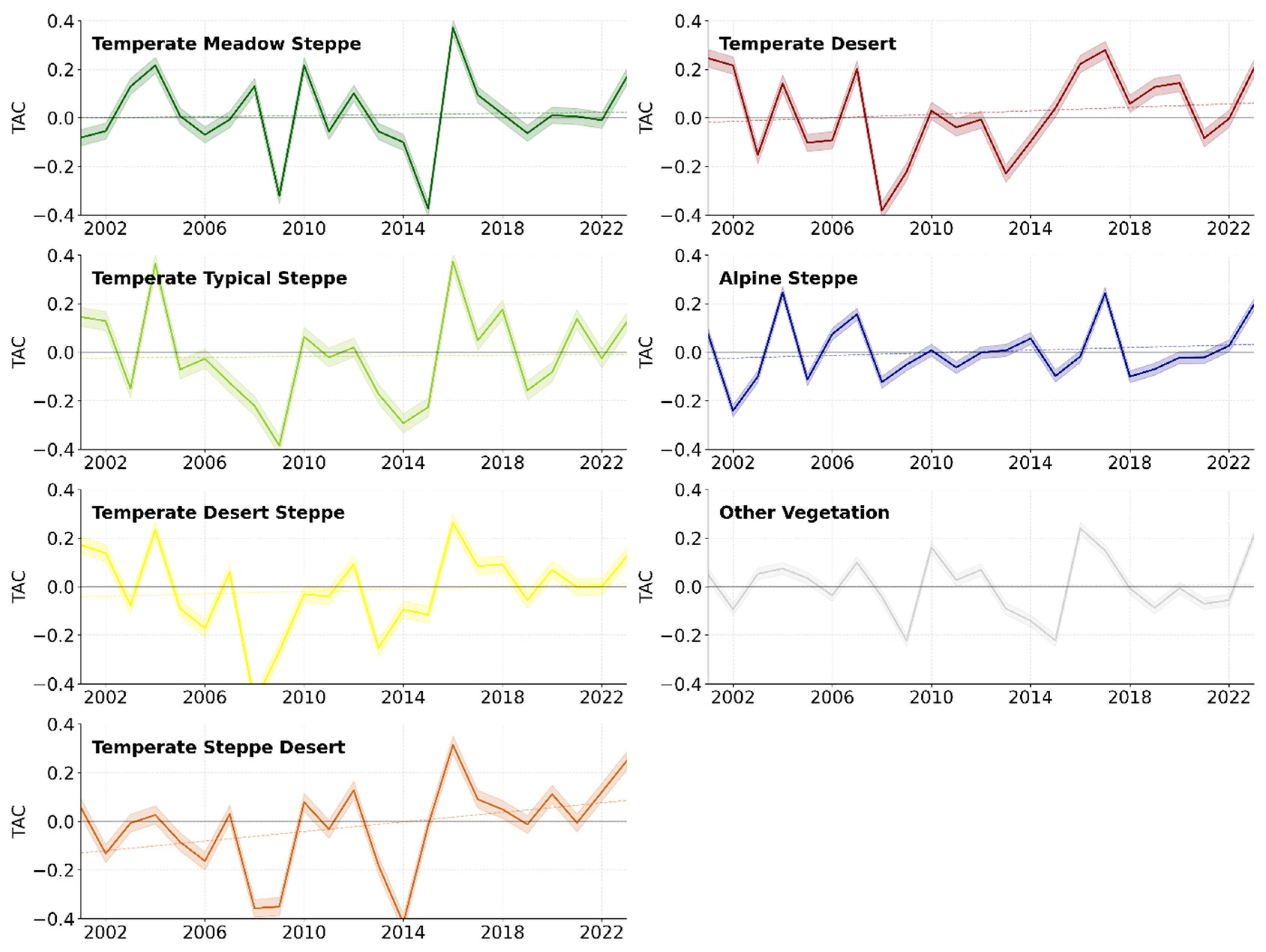
Temporal trajectories of Enhanced TAC (Figure 6) displayed considerable interannual variability across grassland types. Sharp increases in Enhanced TAC—observed in 2004, 2010, 2016, and 2023—indicated abrupt declines in resilience, potentially corresponding to critical slowing down (CSD) events triggered by extreme drought or land use disturbances. These sudden upward shifts may reflect early warning signals of ecosystem instability. Among grassland types, Steppe Desert and Temperate Desert showed pronounced year-to-year volatility, consistent with their exposure to climatic extremes and limited vegetative buffering. Alpine Steppe, by contrast, exhibited more stable dynamics, likely due to thermal constraints that dampened abrupt vegetative fluctuations.
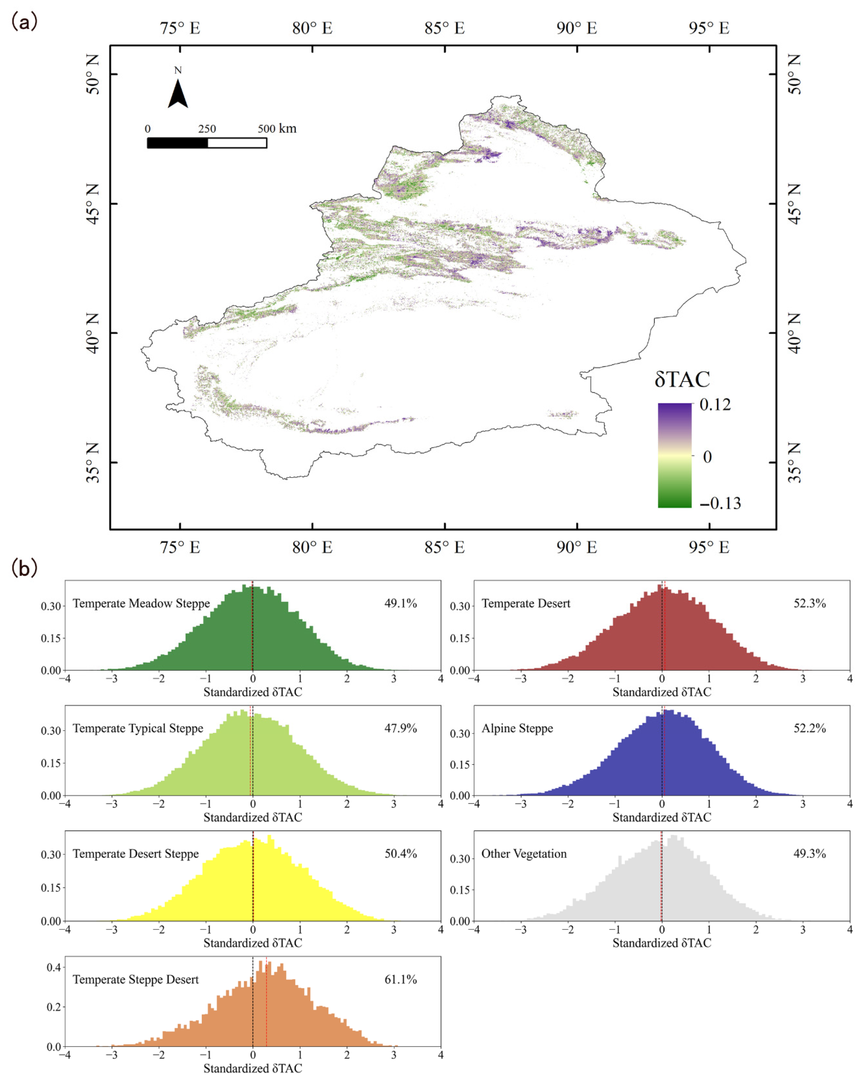
To quantify long-term resilience trends, the linear slope of Enhanced TAC—denoted as δTAC—was computed at the pixel level. Spatial patterns (Figure 7a) showed widespread positive δTAC in southern and eastern regions, signaling ongoing resilience decline in arid transition zones. Meanwhile, negative δTAC in northern and central areas suggests gradual recovery and improved resilience. Distributional analysis of standardized δTAC values across grassland types (Figure 7b) supported these findings. Steppe Desert and Temperate Desert displayed right-skewed distributions, with over 50% of pixels exhibiting positive δTAC, indicative of pervasive resilience degradation. In contrast, Temperate Meadow Steppe and Typical Steppe showed symmetric distributions centered near zero, suggesting relative resilience stability. Alpine Steppe and Other Vegetation types presented broader and more heterogeneous δTAC distributions, reflecting mixed recovery pathways shaped by topographic variation and climatic exposure.
Collectively, the spatial patterns of TAC and δTAC, their temporal dynamics, and grassland-type-specific distributions reveal highly heterogeneous resilience trajectories across Xinjiang’s grassland ecosystems. These divergences reflect complex interactions between vegetation structure, climatic variability, and ecological feedback. The observed spatiotemporal contrasts emphasize that resilience is not uniform but shaped by type-specific environmental thresholds and adaptive capacities. Consequently, effective management under accelerating climate pressures requires localized adaptation strategies and differentiated restoration frameworks tailored to the unique ecological contexts of each grassland system.

3.2. Modeling and Interpretation of Long-Term TAC and δTAC

3.2.1. Modeling and Interpretation of Long-Term TAC

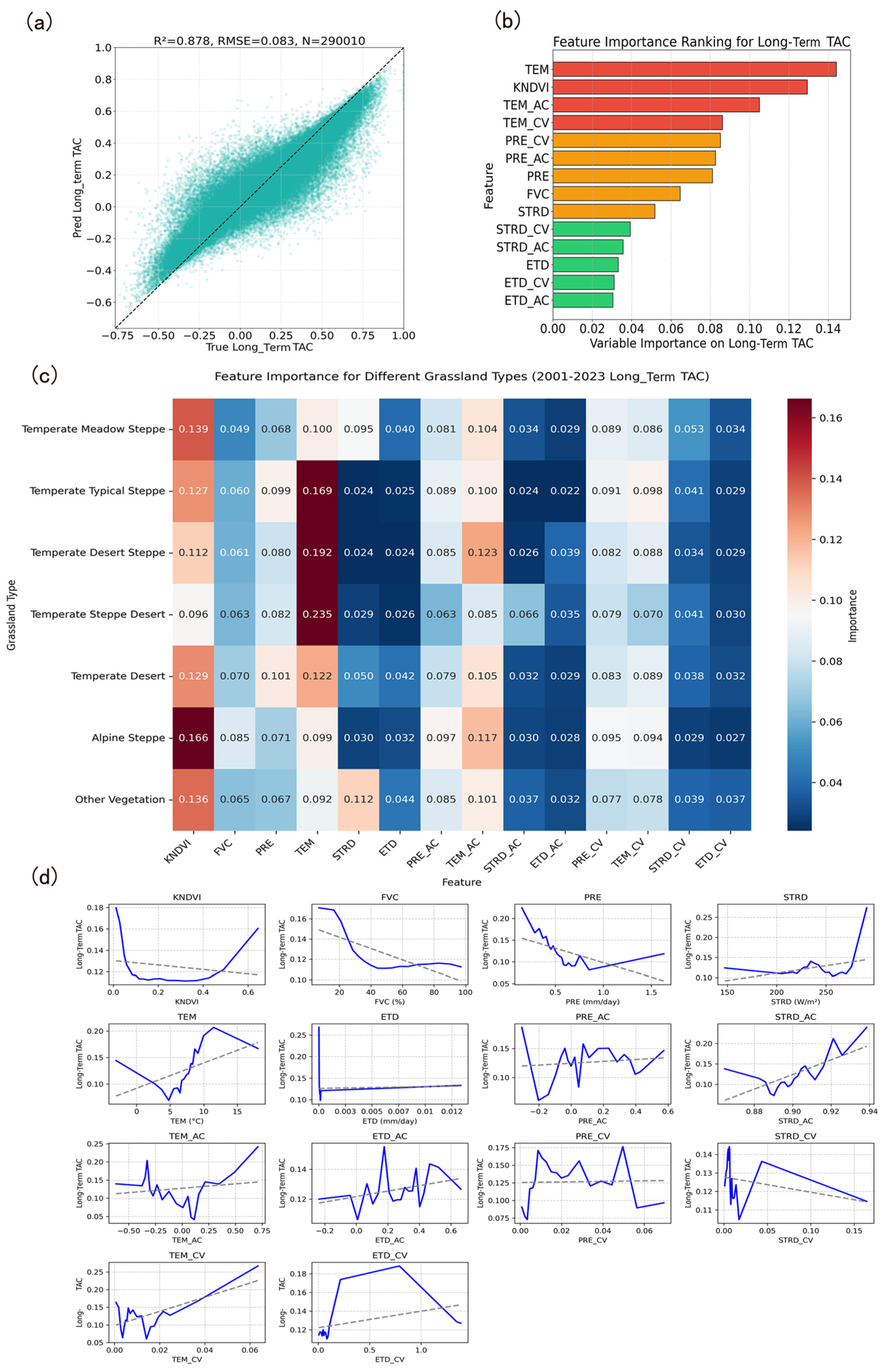
An RF regression model was developed to identify the primary drivers of long-term TAC across grassland ecosystems from 2001 to 2023. Fourteen predictors, including vegetation indices (KNDVI, FVC), climatic means (TEM, PRE, STRD, ETD), and their temporal characteristics (autocorrelation and coefficient of variation), were used. The models were trained separately for each grassland type using an 80:20 train–test split. As shown in Figure 8, the model’s performance and the relative importance of these predictors varied across different grassland types, providing insights into the key drivers of ecosystem resilience.
As shown in Figure 8a, the model demonstrated strong predictive performance (test R2 = 0.878; RMSE = 0.083; n = 290,010), highlighting its power and generalizability. Figure 8b indicates that temperature (TEM) was the most influential predictor, followed by KNDVI, with temperature’s temporal characteristics (TEM_AC and TEM_CV) also playing a key role. Precipitation metrics (PRE_AC and PRE_CV) highlighted the importance of climate memory and variability. Figure 8c shows that KNDVI dominated in Alpine Steppe, while temperature variables had a stronger influence in arid regions, and precipitation was crucial in Temperate Desert Steppe. These differences suggest distinct resilience pathways, emphasizing the need for region-specific restoration strategies. Table S1 (Supplementary Materials) presents a summary of model performance. All models achieved high training R2 (0.92), but testing R2 varied between 0.45 and 0.67, suggesting potential overfitting in some models, which will be discussed in more detail.
Figure 8d reveals a U-shaped relationship between KNDVI and TAC. This suggests that moderate vegetation density was associated with the highest resilience. FVC showed diminishing returns, while precipitation negatively correlated with TAC, particularly below 0.8 mm/day. TAC increased with STRD and TEM, suggesting that higher solar radiation and temperature suppress recovery. Temporal metrics revealed that lower AC values were linked to faster recovery, while CV metrics generally correlated positively with TAC, indicating that higher variability reduces stability. The RF models identified key climatic and vegetative controls on grassland resilience, offering insights for tailored management strategies.
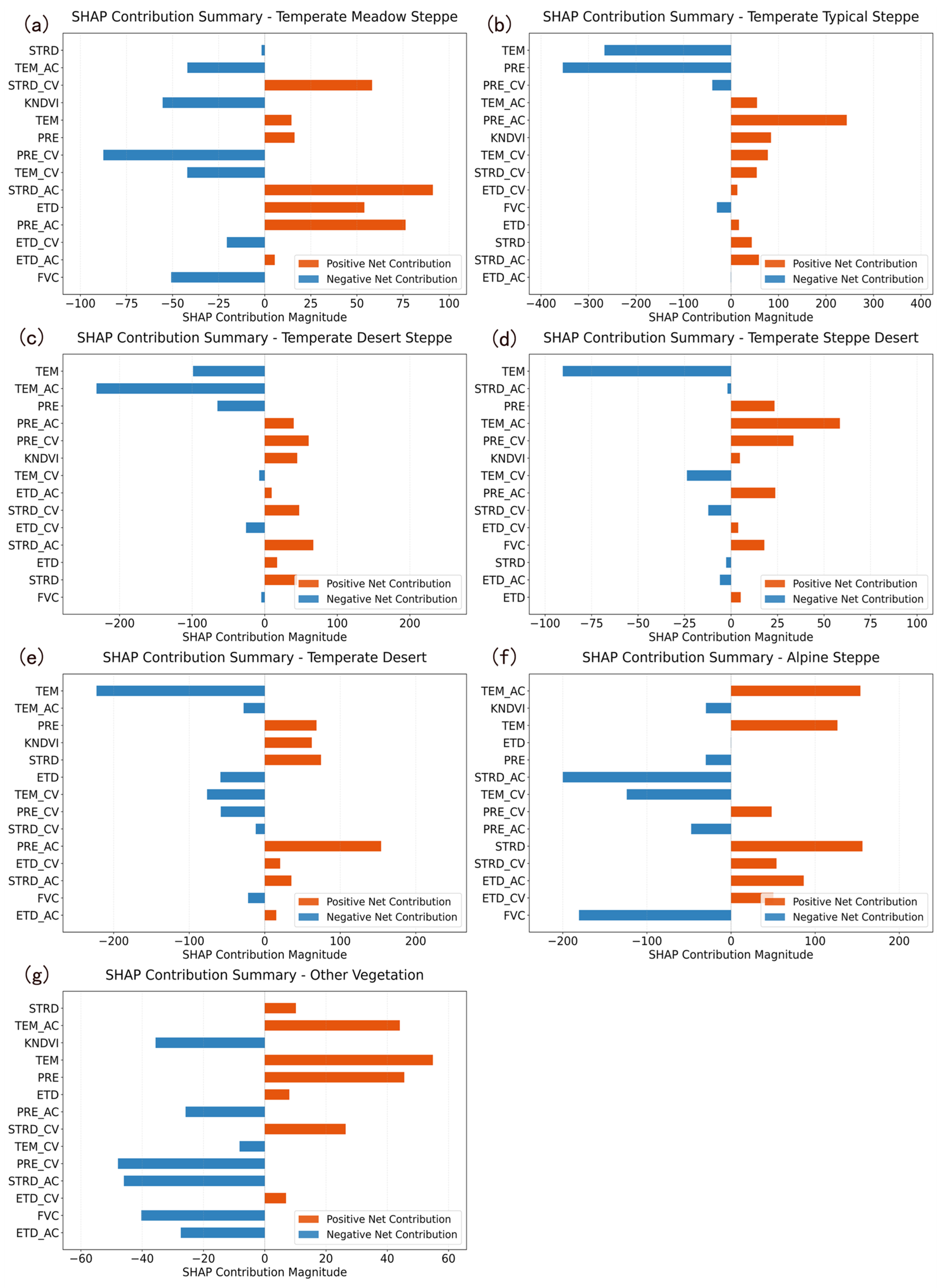
To evaluate the regulatory roles of climatic and vegetative factors on grassland resilience, SHAP analysis was conducted on the outputs of the long-term TAC model. Figure 9 summarizes the marginal effects of individual predictors across seven grassland types. Negative SHAP values indicated enhanced resilience associated with a given variable, while positive values denoted increased TAC and reduced recovery capacity. Variables are sorted from top to bottom according to their total contribution magnitude, defined as the sum of the absolute SHAP values across all years. The underlying SHAP values were computed using an additive decomposition approach applied to the Random Forest model outputs, capturing the marginal effect of each predictor on TAC.
To ensure balanced sampling, stratified subsamples were used for each type: 3000–5000 observations per category, based on sample size and representativeness. SHAP results revealed type-specific patterns. In Temperate Meadow Steppe (Figure 9a), STRD, TEM_AC, STRD_CV, and KNDVI had the most decisive influence, with stable radiation and vegetation cover improving resilience and radiation variability reducing it. Temperature and precipitation supported the recovery in the typical steppe (Figure 9b), while persistent climate conditions (e.g., PRE_AC) weakened elasticity.
In Desert Steppe (Figure 9c) and Steppe Desert (Figure 9d), warming and thermal stability enhanced resilience, while climatic fluctuations weakened it. In Temperate Desert (Figure 9e), rising temperatures promoted resilience, but elevated levels of radiation and precipitation were linked to reduced recovery capacity, possibly due to stress from environmental extremes. Alpine Steppe (Figure 9f) showed resilience suppression under warming, while vegetation indicators (KNDVI, FVC) supported recovery. In Other Vegetation types (Figure 9g), STRD, temperature persistence, and precipitation autocorrelation dominated the response, with vegetation contributing to resilience stability.
Overall, SHAP analysis revealed that vegetation conditions and climate variability jointly regulated ecosystem resilience. These findings underscored the importance of type-specific pathways and highlighted key targets for ecological restoration and adaptive climate responses in grassland systems.

3.2.2. Modeling and Interpretation of δTAC

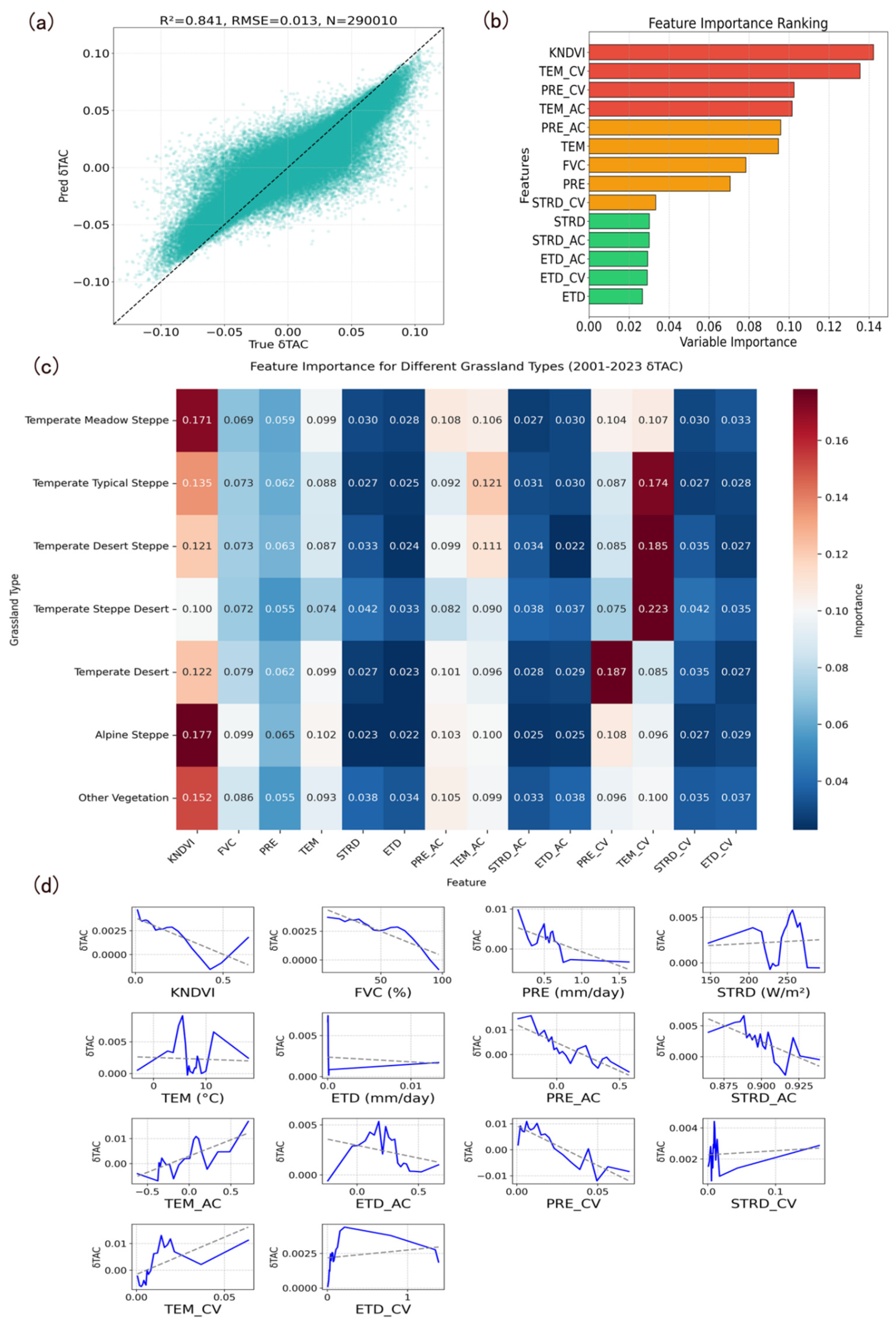
To isolate long-term changes in grassland resilience beyond climatic inertia, this study models δTAC—the linear trend of Enhanced TAC derived after removing climate autocorrelation. The RF regression model, trained on 2001–2023 data, achieved strong overall accuracy (R2 = 0.841; RMSE = 0.013; n = 290,010), though slightly lower than the long-term TAC model, reflecting the greater complexity of trend prediction under shifting environmental regimes. As shown in Figure 10, the model highlighted the key factors influencing δTAC and provided a clearer understanding of the underlying trends in grassland resilience.
KNDVI was identified as the most important predictor of δTAC, followed by interannual variability in temperature and precipitation (TEM_CV, PRE_CV). Unlike the long-term TAC model, climate autocorrelation variables had lower importance, consistent with δTAC’s emphasis on system responsiveness rather than persistence. Feature importance varied across grassland types: KNDVI dominated in alpine and meadow steppes, while temperature variability played a leading role in desert systems. These patterns reflect divergent resilience mechanisms across ecological zones. As shown in Table S2 (Supplementary Materials), model performance varies by grassland type. Temperate Typical Steppe and Desert Steppe showed relatively robust test accuracy (R2 ≈ 0.57), whereas the Alpine Steppe and Other Vegetation types performed poorly (R2 < 0.35), likely due to higher ecological heterogeneity or omitted variables. Despite high training scores for all types, the gap in testing accuracy suggested potential overfitting in complex or data-limited regions. Partial dependence plots revealed the marginal effects of key variables. A U-shaped curve for KNDVI indicated that moderate vegetation density supported more favorable resilience trends, while FVC showed diminishing influence. Precipitation exerted a strong negative effect on δTAC within the range of 0.5–1.5 mm/day, underscoring the stabilizing role of moderate moisture. In contrast, high values of TEM_CV and STRD_CV increased δTAC, suggesting that climate variability weakened resilience trajectories. This δTAC-based modeling framework provided a dynamic complement to long-term TAC analysis, capturing directional trends in resilience loss or recovery. By highlighting the effects of vegetation structure and climatic fluctuation, it supported proactive, spatially targeted grassland management under growing environmental uncertainty.
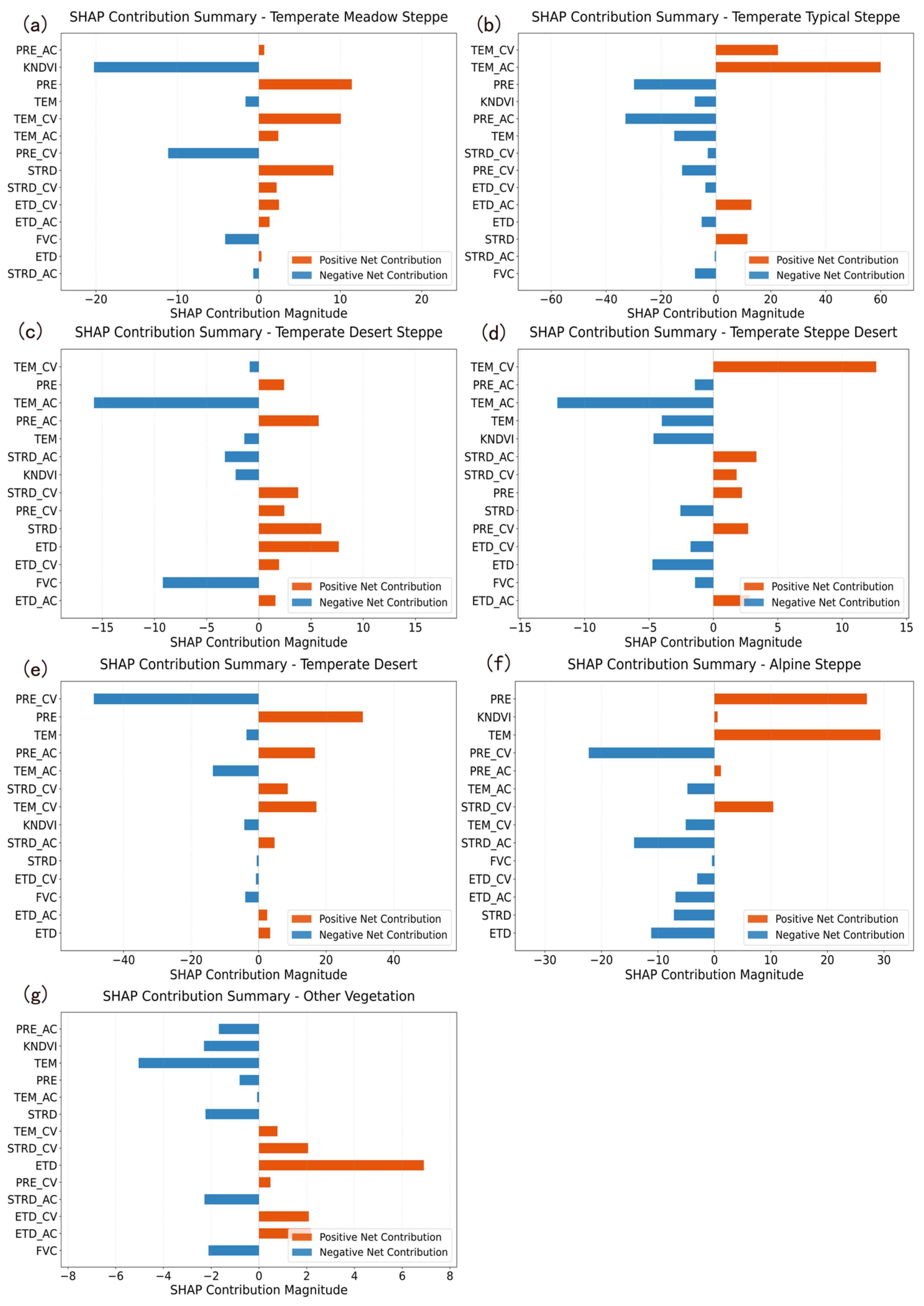
Figure 11 summarizes SHAP results for the δTAC model, illustrating how vegetative and climatic contributions to resilience trends vary across ecosystem types. Compared to the long-term TAC model, δTAC focused on short-term trends and excluded climate memory, enabling clearer insights into how environmental variability shaped resilience dynamics.
In Temperate Meadow Steppe (Figure 11a), resilience benefits from high vegetation activity (KNDVI) and stable precipitation regimes (low PRE_CV). Temperate Typical Steppe (Figure 11b) showed resilience gains from increased temperature (TEM) and precipitation (PRE), while temperature-related persistence (TEM_AC) and variability (TEM_CV) reduced recovery, highlighting sensitivity to unstable thermal regimes. In Temperate Desert Steppe (Figure 11c) and Temperate Steppe Desert (Figure 11d), temperature variability (TEM_CV) emerges as the dominant negative driver, while temperature autocorrelation (TEM_AC) supports resilience by buffering thermal fluctuations. Compared to the long-term TAC model, the positive effect of warming diminished, indicating fewer resilience benefits from rising temperatures under fluctuating conditions.
In Temperate Desert ecosystems (Figure 11e), precipitation (PRE) played the leading positive role, reflecting water limitation as the primary recovery constraint. However, high precipitation variability (PRE_CV) offsets these gains, suggesting that inconsistent moisture inputs hinder long-term resilience. In Alpine Steppe (Figure 11f), temperature-related stress (TEM, TEM_CV) continues to suppress resilience, while precipitation shifted from a neutral or negative role to a positive one, suggesting that warming-induced water availability may support recovery in cold, high-altitude systems. In Other Vegetation types (Figure 11g), climate-related factors—temperature, precipitation, and autocorrelation—consistently inhibit resilience, indicating heightened sensitivity to environmental disturbance. Notably, the evapotranspiration deficit (ETD) appeared as the strongest positive contributor to δTAC, reinforcing that water stress significantly weakens recovery capacity.
Overall, δTAC-based SHAP analysis highlighted the diverging roles of climate variability, vegetation condition, and stress exposure across steppe types. It emphasized the need for tailored adaptation strategies: for instance, stabilizing thermal conditions in Desert Steppes, increasing moisture retention in alpine zones, and mitigating water stress in degraded or mixed-cover landscapes.

4. Discussion

4.1. A TAC-Based Method for Grassland Resilience Evaluation

This study introduces a novel framework combining TAC, Enhanced TAC, and δTAC indicators to assess grassland resilience in Xinjiang from 2001 to 2023. By integrating RF regression with SHAP-based interpretability, the framework disentangles vegetation recovery dynamics from climate memory, enabling type-specific resilience evaluations across diverse ecosystems—from productive meadow steppes to cold alpine zones and arid desert grasslands. The use of SHAP values improves model transparency by quantifying the individual effects of environmental drivers [24,52]. This approach enhances resilience modeling by linking spatial heterogeneity and grassland functional types to their climatic sensitivities, thereby improving diagnostic clarity compared to conventional metrics. In arid and semi-arid environments, increasing climate instability and shifting land use patterns continue to erode ecosystem stability and recovery potential [53]. Accurately identifying the mechanisms underpinning resilience trajectories remains essential for guiding regionally tailored ecological adaptation strategies [54,55]. While most previous studies have concentrated on forest ecosystems [28,33,56,57,58], this work extends resilience assessment to temperate grasslands and alpine systems, particularly within Xinjiang’s ecologically heterogeneous context. By separately modeling long-term TAC and its temporal trend δTAC, the analysis distinguishes between two dimensions of resilience. Long-term TAC reflects the average system inertia over two decades, shaped predominantly by background climatic conditions—particularly mean temperature—and baseline vegetation structure [59]. This suggests that inherent resilience capacity is strongly governed by steady-state thermal regimes and ecosystem biomass levels.
In contrast, δTAC captures the direction and pace of resilience change over time, with its variation more closely linked to climatic instability—namely interannual fluctuations in temperature and precipitation (TEM_CV, PRE_CV)—and vegetation responsiveness [60]. These results imply that while stable climates and dense vegetation support resilience maintenance, increasing climate volatility erodes recovery potential even in structurally intact ecosystems. This differentiation between resilience level and resilience trend provides greater diagnostic clarity and is particularly relevant for climate-sensitive ecosystems such as Desert Steppe, alpine tundra, and transitional zones. The findings align with global studies that report widespread declines in ecosystem resilience under rising climate variability [58,61,62], reinforcing the urgency of integrating temporal climate dynamics into resilience assessment frameworks.

4.2. Grassland-Type Differences in Climate and Vegetation Responses

Model outputs revealed clear divergence in resilience responses among grassland types, shaped by both climatic variability and vegetation characteristics. In relatively humid systems such as Temperate Meadow and Typical Steppe, stability in radiation (STRD_CV) and temperature (TEM_AC), along with higher vegetation indices (e.g., KNDVI), were associated with lower δTAC, indicating stronger resilience under stable hydrothermal conditions [63,64]. However, persistent precipitation signals (PRE_AC) slightly increased δTAC in Typical Steppe, suggesting that overly stable moisture regimes may reduce system elasticity [15]. In more arid types—such as Desert Steppe, Steppe Desert, and Temperate Desert—temperature variability (TEM_CV) emerged as a key destabilizing factor, consistently elevating δTAC. While moderate rainfall variability (PRE_CV) supported resilience in some desert systems, high precipitation levels increased δTAC, implying that excessive water inputs may reduce resilience in ecologically fragile areas [65,66]. These findings echo earlier research indicating a resilience optimum at intermediate precipitation levels, with both drought and excess rainfall increasing vulnerability [34,67,68]. Alpine Steppe systems displayed distinct dynamics: while high vegetation activity (KNDVI and FVC) improved resilience, sustained warming raised δTAC, reflecting long-term sensitivity to thermal stress [69,70,71]. In heterogeneous areas categorized as Other Vegetation types, evapotranspiration deficit (ETD), followed by temperature and precipitation autocorrelation, exerted the strongest influence, highlighting the combined role of climatic memory and water limitation. Overall, the results underscore that grassland resilience trajectories are not uniform but vary systematically with hydrothermal context, vegetation structure, and the nature of climatic fluctuations. Effective adaptation and restoration efforts must therefore account for these biome-specific response patterns rather than applying uniform management strategies.

4.3. Model Limitations and Sampling Considerations

Despite its high training accuracy (R2 > 0.92), the model’s predictive performance in underrepresented or ecologically heterogeneous grassland types—particularly Alpine Steppe (test R2 = 0.450) and Other Vegetation (test R2 = 0.484)—was substantially lower than in more uniform ecosystems. This discrepancy may reflect overfitting or reduced generalizability due to the strong spatial variability and complex degradation pathways in these systems.
To address these challenges, three strategies were adopted. First, we employed an 80:20 train–test split to maximize training data volume. This adjustment significantly improved model performance, especially in high-variance environments such as alpine ecosystems, where sufficient training samples are crucial to capturing ecological complexity. Second, the modeling process was stratified by grassland type, with separate RF models trained for each ecological zone. This type-specific modeling approach helps isolate heterogeneity and improves the ecological interpretability of driver–response relationships within each grassland system. Third, in the SHAP analysis stage, stratified subsampling was applied to mitigate the interpretive bias introduced by imbalanced sample sizes across grassland types. Between 1000 and 5000 samples were selected per type, depending on total availability and representativeness (see Table S3). This approach ensures that dominant vegetation types do not overwhelm the feature attribution process, thereby improving the fairness and comparability of SHAP-derived insights.
Nevertheless, some limitations remain. The reduced performance in Alpine Steppe and other heterogeneous areas may stem from ecological complexity and the absence of key socio-economic drivers such as grazing intensity or land use pressure, which are not captured by remote sensing alone. Future work should consider incorporating anthropogenic variables and refining stratified sampling strategies to improve model generalizability.

4.4. Application Potential for Monitoring and Management

These findings offer valuable guidance for adaptive management in grassland ecosystems and other climate-sensitive biomes. Specifically, identifying resilience drivers for distinct grassland types facilitates the formulation of tailored intervention strategies. For instance, temperature variability was found to be the dominant stressor in Temperate Desert Steppe, underscoring the need for targeted monitoring of thermal anomalies and the development of climate-informed early warning systems. In Alpine Steppe ecosystems, sustained warming was identified as a primary factor contributing to resilience decline, highlighting the importance of strategies that mitigate thermal stress and support vegetation productivity during short growing seasons. As a trend-sensitive indicator, δTAC enables timely detection of resilience degradation and informs spatial prioritization for ecological intervention. Regions exhibiting persistently elevated δTAC values reflect diminished recovery capacity and should be prioritized in restoration planning, outcome-based ecological governance, and compensation frameworks. Importantly, the modeling framework established in this study offers strong transferability to other climate-sensitive ecosystems. While developed in the context of Xinjiang’s grasslands, the TAC-based system—particularly δTAC—can be applied to assess resilience dynamics in shrublands, wetlands, savannas, and dry forests, where climatic variability and vegetation responses are similarly interlinked. This framework supports the detection of resilience thresholds, refinement of land use practices such as rotational grazing, and long-term ecosystem monitoring under environmental change. By integrating both structural and temporal dimensions of ecosystem resilience, it enhances early detection of resilience decline and informs spatially explicit, regionally adaptive management strategies. Future research could further generalize this approach by incorporating additional dynamic indicators and socio-ecological variables—such as grazing intensity, land use transitions, and institutional governance—thereby enabling a more holistic understanding of resilience mechanisms. Such multidimensional integration offers a robust and scalable pathway for resilience-informed ecosystem management across diverse landscapes.

5. Conclusions

This study developed a multidimensional diagnostic framework to assess the resilience of grassland ecosystems in Xinjiang by integrating TAC, Enhanced TAC, and δTAC indicators with RF modeling and SHAP-based explainability. The results revealed significant spatial and typological differences in resilience status and trends. Vegetation activity, climate variability, and temperature fluctuations were identified as dominant drivers, while δTAC proved effective in capturing early warning signals of resilience decline, enabling the identification of high-risk areas.
The proposed framework provides a practical basis for ecological decision-making. First, it can assist local authorities in delineating high-priority zones for restoration investment, especially in grassland types with consistent declines in δTAC. Second, it supports the formulation of differentiated management strategies—such as rotational grazing schemes or grazing bans—tailored to ecosystem sensitivity levels. Third, the framework can inform performance-based ecological compensation mechanisms, where subsidy allocations are dynamically adjusted according to spatial patterns of degradation risk and resilience loss. Lastly, by integrating early warning indicators into routine monitoring systems, land managers can adopt more timely and cost-effective responses to prevent irreversible ecosystem shifts. Future work should explore integrating socio-economic drivers, such as grazing intensity and land tenure patterns, to improve model generalizability and inform cross-sectoral policy. Expanding this framework to other arid and semi-arid regions would further enhance its utility for national ecological restoration programs.
To improve predictive robustness and practical applicability, future efforts should consider the following: (1) incorporating anthropogenic variables such as grazing intensity or infrastructure proximity; (2) applying stratified sampling or oversampling methods to balance ecological types; (3) refining algorithms through cross-validation, ensemble averaging, or Bayesian optimization. Additionally, the integration of critical slowing down (CSD) metrics and lagged climate autocorrelation indicators may enhance the framework’s ability to detect resilience thresholds more reliably. Overall, this study provides a replicable approach to monitoring ecosystem resilience and offers a science-based tool to support targeted, data-informed grassland governance in arid and semi-arid regions.

Supplementary Materials

The following supporting information can be downloaded at: https://www.mdpi.com/article/10.3390/rs17162749/s1, Table S1: Long-term TAC model performance; Table S2: δTAC model performance; Table S3: Stratified sampling scheme for SHAP analysis across grassland types.

Author Contributions

R.L. conducted data processing, modeling, and wrote the first draft. Y.Y. designed the research and supervised the study. I.M. and M.W. contributed to ecological interpretation and manuscript revision. Z.G., Y.L., X.D., J.H., L.S., C.L., and R.Y. supported data collection, figure generation, and the literature review. All authors contributed substantially to manuscript revision and approved the final version. All authors have read and agreed to the published version of the manuscript.

Funding

This research has been funded by the National Key Research and Development Program of China (2023YFF0805603) and the Key Research and Development Program of Xinjiang (2022B01032-4).

Data Availability Statement

The data supporting the findings of this study have been deposited in Figshare [72] and are publicly available via the following DOI: https://doi.org/10.6084/m9.figshare.28804409.v2 (accessed on 5 August 2025).

Acknowledgments

During the preparation of this work, the authors used ChatGPT-4o (OpenAI) to improve language clarity and grammar. After using this tool, the authors reviewed and edited the content as needed and take full responsibility for the content of the publication.

Conflicts of Interest

The authors declare no conflicts of interest.

References

  1. Poulter, B.; Frank, D.; Ciais, P.; Myneni, R.B.; Andela, N.; Bi, J.; Broquet, G.; Canadell, J.G.; Chevallier, F.; Liu, Y.Y.; et al. Contribution of semi-arid ecosystems to interannual variability of the global carbon cycle. Nature 2014, 509, 600–603. [Google Scholar] [CrossRef]
  2. Díaz, S.; Zafra-Calvo, N.; Purvis, A.; Verburg, P.H.; Obura, D.; Leadley, P.; Chaplin-Kramer, R.; De Meester, L.; Dulloo, E.; Martín-López, B.; et al. Set ambitious goals for biodiversity and sustainability. Science 2020, 370, 411–413. [Google Scholar] [CrossRef]
  3. Environment Programme. Intergovernmental Panel on Climate Change Climate Change 2021: The Physical Science Basis. In Proceedings of the Contribution of Working Group I to the Sixth Assessment Report of the Intergovernmental Panel on Climate Change, Cambridge, UK; New York, NY, USA, 9 August 2021; p. 2391. [Google Scholar]
  4. Du, B.; Zhen, L.; Yan, H.; De Groot, R. Effects of Government Grassland Conservation Policy on Household Livelihoods and Dependence on Local Grasslands: Evidence from Inner Mongolia, China. Sustainability 2016, 8, 1314. [Google Scholar] [CrossRef]
  5. Lan, X.; Zhang, Q.; Xue, H.; Liang, H.; Wang, B.; Wang, W. Linking sustainable livelihoods with sustainable grassland use and conservation: A case study from rural households in a semi-arid grassland area, China. Land Use Policy 2021, 101, 105186. [Google Scholar] [CrossRef]
  6. Hou, Q.; Ji, Z.; Yang, H.; Yu, X. Impacts of climate change and human activities on different degraded grassland based on NDVI. Sci. Rep. 2022, 12, 15918. [Google Scholar] [CrossRef] [PubMed]
  7. United Nations Convention to Combat Desertification Global. Land Outlook: Rangeland Degradation Threatens Food Security and Ecosystem Health; UNCCD: Bonn, Germany, 2022. [Google Scholar]
  8. Drake, J.E.; Tjoelker, M.G.; Vårhammar, A.; Medlyn, B.E.; Reich, P.B.; Leigh, A.; Pfautsch, S.; Blackman, C.J.; López, R.; Aspinwall, M.J.; et al. Trees tolerate an extreme heatwave via sustained transpirational cooling and increased leaf thermal tolerance. Glob. Change Biol. 2018, 24, 2390–2402. [Google Scholar] [CrossRef] [PubMed]
  9. Byrne, B.; Liu, J.; Lee, M.; Yin, Y.; Bowman, K.W.; Miyazaki, K.; Norton, A.J.; Joiner, J.; Pollard, D.F.; Griffith, D.W.T.; et al. The Carbon Cycle of Southeast Australia During 2019–2020: Drought, Fires, and Subsequent Recovery. AGU Adv. 2021, 2, e2021AV000469. [Google Scholar] [CrossRef]
  10. Tao, S.; Wigneron, J.-P.; Chave, J.; Tang, Z.; Wang, Z.; Zhu, J.; Guo, Q.; Liu, Y.Y.; Ciais, P. Little evidence that Amazonian rainforests are approaching a tipping point. Nat. Clim. Change 2023, 13, 1317–1320. [Google Scholar] [CrossRef]
  11. Su, J.; Zhao, Y.; Xu, F.; Bai, Y. Multiple global changes drive grassland productivity and stability: A meta-analysis. J. Ecol. 2022, 110, 2850–2869. [Google Scholar] [CrossRef]
  12. Bangira, T.; Mutanga, O.; Sibanda, M.; Dube, T.; Mabhaudhi, T. Remote Sensing Grassland Productivity Attributes: A Systematic Review. Remote Sens. 2023, 15, 2043. [Google Scholar] [CrossRef]
  13. She, Y.; Li, X.; Zhang, J.; Zhou, H. Effects of soil characteristics on grassland productivity in long-term artificial grassland establishment. Glob. Ecol. Conserv. 2024, 54, e03136. [Google Scholar] [CrossRef]
  14. Carpenter, S.; Walker, B.; Anderies, J.M.; Abel, N. From metaphor to measurement: Resilience of what to what? Ecosystems 2001, 4, 765–781. [Google Scholar] [CrossRef]
  15. Scheffer, M.; Bascompte, J.; Brock, W.A.; Brovkin, V.; Carpenter, S.R.; Dakos, V.; Held, H.; van Nes, E.H.; Rietkerk, M.; Sugihara, G. Early-warning signals for critical transitions. Nature 2009, 461, 53–59. [Google Scholar] [CrossRef] [PubMed]
  16. Suding, K.N.; Gross, K.L.; Houseman, G.R. Alternative states and positive feedbacks in restoration ecology. Trends Ecol. Evol. 2004, 19, 46–53. [Google Scholar] [CrossRef]
  17. Reynolds, J.F.; Smith, D.M.S.; Lambin, E.F.; Turner, B.L.; Mortimore, M.; Batterbury, S.P.J.; Downing, T.E.; Dowlatabadi, H.; Fernández, R.J.; Herrick, J.E.; et al. Global Desertification: Building a Science for Dryland Development. Science 2007, 316, 847–851. [Google Scholar] [CrossRef] [PubMed]
  18. Angeler, D.G.; Allen, C.R. Quantifying resilience. J. Appl. Ecol. 2016, 53, 617–624. [Google Scholar] [CrossRef]
  19. Dakos, V.; Carpenter, S.R.; Brock, W.A.; Ellison, A.M.; Guttal, V.; Ives, A.R.; Kéfi, S.; Livina, V.; Seekell, D.A.; van Nes, E.H.; et al. Methods for Detecting Early Warnings of Critical Transitions in Time Series Illustrated Using Simulated Ecological Data. PLoS ONE 2012, 7, e41010. [Google Scholar] [CrossRef] [PubMed]
  20. Olden, J.D.; Lawler, J.J.; Poff, N.L. Machine learning methods without tears: A primer for ecologists. Q. Rev. Biol. 2008, 83, 171–193. [Google Scholar] [CrossRef] [PubMed]
  21. Peters, D.P.C.; Havstad, K.M.; Cushing, J.; Tweedie, C.; Fuentes, O.; Villanueva-Rosales, N. Harnessing the power of big data: Infusing the scientific method with machine learning to transform ecology. Ecosphere 2014, 5, art67. [Google Scholar] [CrossRef]
  22. Reichstein, M.; Camps-Valls, G.; Stevens, B.; Jung, M.; Denzler, J.; Prabhat, C.N. Deep learning and process understanding for data-driven Earth system science. Nature 2019, 566, 195–204. [Google Scholar] [CrossRef]
  23. Ribeiro, M.T.; Singh, S.; Guestrin, C. “Why Should I Trust You?”: Explaining the Predictions of Any Classifier. In Proceedings of the 22nd ACM SIGKDD International Conference on Knowledge Discovery and Data Mining, San Francisco, CA, USA, 16 February 2016; pp. 1135–1144. [Google Scholar]
  24. Lundberg, S.M.; Lee, S.-I. A unified approach to interpreting model predictions. In Proceedings of the 31st International Conference on Neural Information Processing Systems, Long Beach, CA, USA, 4–9 December 2017; pp. 4768–4777. [Google Scholar]
  25. Lipton, Z.C. The mythos of model interpretability. Commun. ACM 2018, 61, 36–43. [Google Scholar] [CrossRef]
  26. Lundberg, S.M.; Erion, G.G.; Lee, S.-I.J.A. Consistent Individualized Feature Attribution for Tree Ensembles. arXiv 2018, arXiv:1802.03888. [Google Scholar]
  27. Cha, Y.; Shin, J.; Go, B.; Lee, D.S.; Kim, Y.; Kim, T.; Park, Y.S. An interpretable machine learning method for supporting ecosystem management: Application to species distribution models of freshwater macroinvertebrates. J. Environ. Manag. 2021, 291, 112719. [Google Scholar] [CrossRef] [PubMed]
  28. Chen, J.; Wang, S.; Shi, H.; Chen, B.; Wang, J.; Zheng, C.; Zhu, K. Radiation and temperature dominate the spatiotemporal variability in resilience of subtropical evergreen forests in China. Front. For. Glob. Change 2023, 6, 1166481. [Google Scholar] [CrossRef]
  29. Delaney, J.T.; Larson, D.M. Using explainable machine learning methods to evaluate vulnerability and restoration potential of ecosystem state transitions. Conserv. Biol. 2024, 38, e14203. [Google Scholar] [CrossRef]
  30. Holling, C.S. Systematics. Resilience and Stability of Ecological Systems. Annu. Rev. Ecol. Syst. 1973, 4, 1–23. [Google Scholar] [CrossRef]
  31. Pimm, S.L. The complexity and stability of ecosystems. Nature 1984, 307, 321–326. [Google Scholar] [CrossRef]
  32. Resilience, A. Resilience Alliance: A New Perspective on Ecosystem Management and Sustainability; Resilience Alliance: Stockholm, Sweden, 2002. [Google Scholar]
  33. Forzieri, G.; Dakos, V.; McDowell, N.G.; Ramdane, A.; Cescatti, A. Emerging signals of declining forest resilience under climate change. Nature 2022, 608, 534–539. [Google Scholar] [CrossRef]
  34. Smith, T.; Boers, N. Global vegetation resilience linked to water availability and variability. Nat. Commun. 2023, 14, 498. [Google Scholar] [CrossRef] [PubMed]
  35. Fan, X.; Hao, X.; Hao, H.; Zhang, J.; Li, Y. Comprehensive Assessment Indicator of Ecosystem Resilience in Central Asia. Water 2021, 13, 124. [Google Scholar] [CrossRef]
  36. Zhang, S.; Yang, Y.; Wu, X.; Li, X.; Shi, F. Postdrought Recovery Time Across Global Terrestrial Ecosystems. J. Geophys. Res. Biogeosci. 2021, 126, e2020JG005699. [Google Scholar] [CrossRef]
  37. Wu, J.; Sun, Z.; Yao, Y.; Liu, Y. Trends of Grassland Resilience under Climate Change and Human Activities on the Mongolian Plateau. Remote Sens. 2023, 15, 2984. [Google Scholar] [CrossRef]
  38. Zhang, Y.; Liu, X.; Jiao, W.; Wu, X.; Zeng, X.; Zhao, L.; Wang, L.; Guo, J.; Xing, X.; Hong, Y. Spatial Heterogeneity of Vegetation Resilience Changes to Different Drought Types. Earth’s Future 2023, 11, e2022EF003108. [Google Scholar] [CrossRef]
  39. Paudel, A.; Chen, Y.-H.; Brodylo, D.; Markwith, S.H. Spatial Monte Carlo Simulation and Analysis of Climate Change Enhanced Fire and Projected Landscape-Scale Variation in Vegetation Heterogeneity. J. Geovis. Spat. Anal. 2024, 8, 22. [Google Scholar] [CrossRef]
  40. Zhang, S.; Lei, J.; Tong, Y.; Zhang, X.; Lu, D.; Fan, L.; Duan, Z. Temporal and spatial responses of ecological resilience to climate change and human activities in the economic belt on the northern slope of the Tianshan Mountains, China. J. Arid Land 2023, 15, 1245–1268. [Google Scholar] [CrossRef]
  41. Chen, Y.; Fang, G.; Li, Z.; Zhang, X.; Gao, L.; Elbeltagi, A.; Shaer, H.E.; Duan, W.; Wassif, O.M.A.; Li, Y.; et al. The Crisis in Oases: Research on Ecological Security and Sustainable Development in Arid Regions. Annu. Rev. Environ. Resour. 2024, 49, 1–20. [Google Scholar] [CrossRef]
  42. He, X.; Zhang, L.; Lu, Y.; Chai, L. Spatiotemporal Variations of Vegetation and Its Response to Climate Change and Human Activities in Arid Areas—A Case Study of the Shule River Basin, Northwestern China. Forests 2024, 15, 1147. [Google Scholar] [CrossRef]
  43. Yang, J.; Huang, X. The 30 m annual land cover datasets and its dynamics in China from 1985 to 2023. Earth Syst. Sci. Data 2024, 13, 3907–3925. [Google Scholar] [CrossRef]
  44. Yu, G.; Lu, C.; Xie, G.; Luo, Z.; Yang, L. Grassland ecosystem services and their economic evaluation in qinghai-tibetan plateau based on RS and GIS. In Proceedings of the 2005 IEEE International Geoscience and Remote Sensing Symposium, 2005. IGARSS’05, Seoul, Republic of Korea, 29–29 July 2005; Volume 4, pp. 2961–2964. [Google Scholar]
  45. Wan, Q.; Meng, Y.; Xie, X.; Zhang, X.; Han, C.; Li, J. An analysis on spatiotemporal differentiation characteristics of the ecosystem service value of the Xinjiang Production and Construction Corps. Shengtai Xuebao Acta Ecol. Sin. 2014, 34, 7057–7066. [Google Scholar] [CrossRef]
  46. China Meteorological Administration. China Ground Climate Data Daily Dataset (SURF_CLI_CHN_MUL_DAY); Version 1.0; China Meteorological Administration: Beijing, China, 2014. Available online: http://data.cma.cn/ (accessed on 11 August 2024).
  47. China Meteorological Administration. China Ground Climate Data Daily Dataset (SURF_CLI_CHN_MUL_DAY); Version 3.0; China Meteorological Administration: Beijing, China, 2019. Available online: http://data.cma.cn/ (accessed on 11 August 2024).
  48. Hersbach, H.; Bell, B.; Berrisford, P.; Biavati, G.; Horányi, A.; Muñoz Sabater, J.; Nicolas, J.; Peubey, C.; Radu, R.; Rozum, I.; et al. ERA5 hourly data on single levels from 1940 to present. Copernicus Climate Change Service (C3S) Climate Data Store (CDS), 2023. Available online: https://cds.climate.copernicus.eu (accessed on 3 September 2024).
  49. Didan, K. MOD13A2 MODIS/Terra Vegetation Indices 16-Day L3 Global 1km SIN Grid V006. Available online: https://www.earthdata.nasa.gov/data/catalog/lpcloud-mod13a2-006 (accessed on 6 August 2024).
  50. Gao, J.; Shi, Y.; Zhang, H.; Chen, X.; Zhang, W.; Shen, W.; Xiao, T.; Zhang, Y. China Regional 250 m Fractional Vegetation Cover Dataset (2000–2023). National Tibetan Plateau Data Center, 2024. Available online: https://data.tpdc.ac.cn (accessed on 19 October 2024).
  51. Tang, J.; Xu, X.; Zhang, A.; Zhang, N. Spatial and Temporal Variation of Temperate Grassland Types in Eurasia—China Regional Three-Level Classification (1980s). National Tibetan Plateau Data Center, 2020. Available online: https://data.tpdc.ac.cn/zh-hans/data/20722773-9955-4d6e-a761-ed23814aca41 (accessed on 14 December 2024).
  52. Saeed, W.; Omlin, C. Explainable AI (XAI): A systematic meta-survey of current challenges and future opportunities. Knowl. Based Syst. 2023, 263, 110273. [Google Scholar] [CrossRef]
  53. Berdugo, M.; Delgado-Baquerizo, M.; Soliveres, S.; Hernández-Clemente, R.; Zhao, Y.; Gaitán, J.J.; Gross, N.; Saiz, H.; Maire, V.; Lehmann, A.; et al. Global ecosystem thresholds driven by aridity. Science 2020, 367, 787–790. [Google Scholar] [CrossRef]
  54. Scheffer, M.; Carpenter, S.; Foley, J.A.; Folke, C.; Walker, B. Catastrophic shifts in ecosystems. Nature 2001, 413, 591–596. [Google Scholar] [CrossRef]
  55. Mayer, A.L.; Rietkerk, M. The Dynamic Regime Concept for Ecosystem Management and Restoration. BioScience 2004, 54, 1013–1020. [Google Scholar] [CrossRef]
  56. Stevens-Rumann, C.S.; Kemp, K.B.; Higuera, P.E.; Harvey, B.J.; Rother, M.T.; Donato, D.C.; Morgan, P.; Veblen, T.T. Evidence for declining forest resilience to wildfires under climate change. Ecol. Lett. 2018, 21, 243–252. [Google Scholar] [CrossRef]
  57. Li, J.; He, B.; Ahmad, S.; Mao, W. Leveraging explainable machine learning models to assess forest health: A case study in Hainan, China. Ecol. Evol. 2023, 13, e10558. [Google Scholar] [CrossRef]
  58. Boulton, C.A.; Lenton, T.M.; Boers, N. Pronounced loss of Amazon rainforest resilience since the early 2000s. Nat. Clim. Change 2022, 12, 271–278. [Google Scholar] [CrossRef]
  59. Kéfi, S.; Guttal, V.; Brock, W.A.; Carpenter, S.R.; Ellison, A.M.; Livina, V.N.; Seekell, D.A.; Scheffer, M.; van Nes, E.H.; Dakos, V. Early Warning Signals of Ecological Transitions: Methods for Spatial Patterns. PLoS ONE 2014, 9, e92097. [Google Scholar] [CrossRef]
  60. Hughes, T.P.; Kerry, J.T.; Connolly, S.R.; Baird, A.H.; Eakin, C.M.; Heron, S.F.; Hoey, A.S.; Hoogenboom, M.O.; Jacobson, M.; Liu, G.; et al. Ecological memory modifies the cumulative impact of recurrent climate extremes. Nat. Clim. Change 2019, 9, 40–43. [Google Scholar] [CrossRef]
  61. Xu, C.; Ke, Y.; Zhou, W.; Luo, W.; Ma, W.; Song, L.; Smith, M.D.; Hoover, D.L.; Wilcox, K.R.; Fu, W.; et al. Resistance and resilience of a semi-arid grassland to multi-year extreme drought. Ecol. Indic. 2021, 131, 108139. [Google Scholar] [CrossRef]
  62. Yao, Y.; Liu, Y.; Fu, F.; Song, J.; Wang, Y.; Han, Y.; Wu, T.; Fu, B. Declined terrestrial ecosystem resilience. Glob. Change Biol. 2024, 30, e17291. [Google Scholar] [CrossRef]
  63. Liu, L.; Gou, X.; Wang, X.; Yang, M.; Qie, L.; Pang, G.; Wei, S.; Zhang, F.; Li, Y.; Wang, Q.; et al. Relationship between extreme climate and vegetation in arid and semi-arid mountains in China: A case study of the Qilian Mountains. Agric. For. Meteorol. 2024, 348, 109938. [Google Scholar] [CrossRef]
  64. Wei, M.; Jiao, L.; Zhang, P.; Xue, R.; Wang, X.; Li, Q.; Jin, M. Spatial and temporal characteristics of vegetation resilience to drought in China. Sci. China Earth Sci. 2025, 68, 2310–2327. [Google Scholar] [CrossRef]
  65. Hossain, M.L.; Li, J.; Lai, Y.; Beierkuhnlein, C. Long-term evidence of differential resistance and resilience of grassland ecosystems to extreme climate events. Environ. Monit. Assess. 2023, 195, 734. [Google Scholar] [CrossRef] [PubMed]
  66. Wang, C.; Vera-Vélez, R.; Lamb, E.G.; Wu, J.; Ren, F. Global pattern and associated drivers of grassland productivity sensitivity to precipitation change. Sci. Total Environ. 2022, 806, 151224. [Google Scholar] [CrossRef]
  67. Cao, W.; Bai, J.; Yu, L. Grassland-type ecosystem stability in China differs under the influence of drought and wet events. J. Arid. Land 2024, 16, 615–631. [Google Scholar] [CrossRef]
  68. Wang, Y.; Klaus, V.H.; Gilgen, A.K.; Buchmann, N. Temperate grasslands under climate extremes: Effects of plant diversity on ecosystem services. Agric. Ecosyst. Environ. 2025, 379, 109372. [Google Scholar] [CrossRef]
  69. Shen, M.; Tang, Y.; Chen, J.; Zhu, X.; Zheng, Y. Influences of temperature and precipitation before the growing season on spring phenology in grasslands of the central and eastern Qinghai-Tibetan Plateau. Agric. For. Meteorol. 2011, 151, 1711–1722. [Google Scholar] [CrossRef]
  70. Duan, H.; Xue, X.; Wang, T.; Kang, W.; Liao, J.; Liu, S. Spatial and Temporal Differences in Alpine Meadow, Alpine Steppe and All Vegetation of the Qinghai-Tibetan Plateau and Their Responses to Climate Change. Remote Sens. 2021, 13, 669. [Google Scholar] [CrossRef]
  71. Li, Y.; Gong, J.; Zhang, Y.; Gao, B. NDVI-Based Greening of Alpine Steppe and Its Relationships with Climatic Change and Grazing Intensity in the Southwestern Tibetan Plateau. Land 2022, 11, 975. [Google Scholar] [CrossRef]
  72. Liu, R. Grassland Resilience Assessment Using Explainable Machine Learning in Arid Ecosystems of Northwest China (2001–2023). Figshare. Dataset. 2025. Available online: https://figshare.com/articles/dataset/Grassland_Resilience_Assessment_Using_Explainable_Machine_Learning_in_Arid_Ecosystems_of_Northwest_China_2001_2023_/28804409/2 (accessed on 5 August 2025).
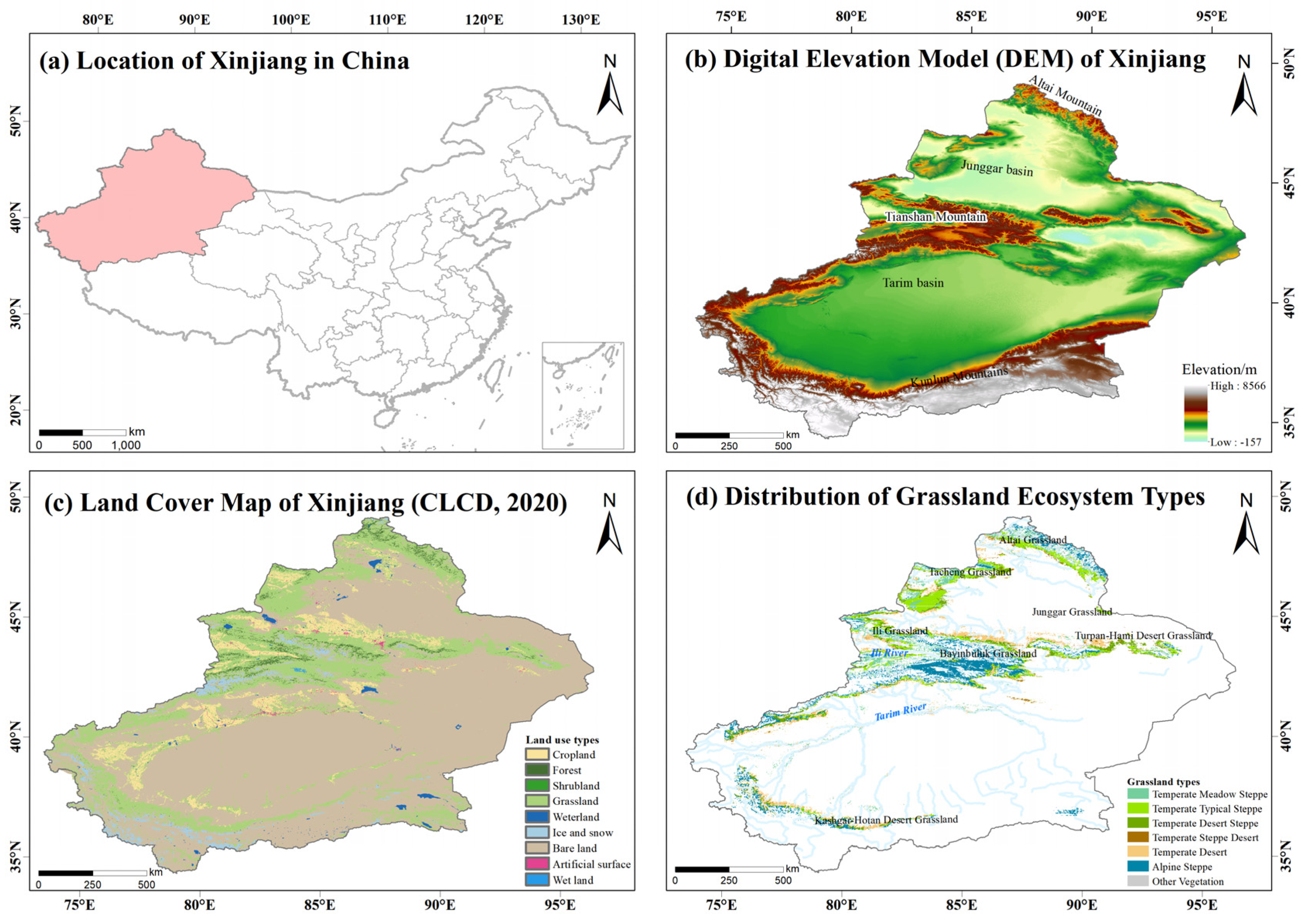
Figure 1. Overview of the study area in Xinjiang. (a) Geographic location of Xinjiang within China. (b) Digital Elevation Model (DEM) showing elevation patterns, the Tianshan Mountains, Junggar Basin, and Tarim Basin. (c) Land cover classification based on the China Land Cover Dataset (CLCD, 2020) [43], including cropland, forest, shrubland, grassland, and bare land. (d) Distribution of seven grassland ecosystem types. All spatial layers were resampled to 1 km resolution and processed using ArcGIS 10.8.
Remotesensing 17 02749 g001
Figure 2. Boxplots illustrating variations in key environmental and vegetation variables across seven dominant grassland types in Xinjiang from 2001 to 2023. (a) Kernel Normalized Difference Vegetation Index (KNDVI), (b) Fractional Vegetation Cover (FVC), (c) mean annual temperature (°C), (d) mean daily precipitation (mm/day), (e) surface total downward radiation (W·m−2), (f) daily evapotranspiration deficit (ETD, mm/day). Grassland types: 1—Temperate Meadow Steppe; 2—Temperate Typical Steppe; 3—Temperate Desert Steppe; 4—Temperate Steppe Desert; 5—Temperate Desert; 6—Alpine Steppe; 7—Other Vegetation. Boxes show interquartile ranges (IQRs), horizontal lines indicate medians, whiskers extend to 1.5 × IQR. This figure highlights environmental gradients shaping grassland resilience in arid northwestern China.
Remotesensing 17 02749 g002
Figure 3. Spatial distribution of key climate and vegetation variables in Xinjiang, 2001–2023. (a) Kernel Normalized Difference Vegetation Index (KNDVI); (b) Fractional Vegetation Cover (FVC); (c) mean annual air temperature (TEM, °C); (d) mean annual precipitation (PRE, mm/day); (e) surface total radiation downward (STRD, W/m2); (f) evapotranspiration deficit (ETD, mm/day).
Remotesensing 17 02749 g003
Figure 4. SHAP value waterfall diagram showing individual feature contributions to model prediction. Features: TEM + 0.15, PRE − 0.08, ETD − 0.06, STRD + 0.05. Baseline 0.00 is the mean prediction. Final output exceeds baseline by +0.06 units. Green bars indicate positive contributions, red bars negative contributions.
Remotesensing 17 02749 g004
Figure 5. Spatial patterns and distribution characteristics of long-term vegetation temporal autocorrelation (TAC) in Xinjiang’s grasslands from 2001 to 2023. (a) Long-term TAC map: Blue indicates higher TAC (lower resilience), yellow shows lower TAC (higher resilience). (b) TAC change map (2001–2010 vs. 2011–2023): Red denotes resilience decline, green indicates improvement. (c) Standardized TAC distributions for seven grassland types. Dashed lines: Black = mean (zero), red = median. Percentages show pixels with TAC > 0 (lower than average resilience).
Remotesensing 17 02749 g005
Figure 6. Temporal dynamics of Enhanced Temporal Autocorrelation (TAC) across grassland types in Xinjiang from 2001 to 2023. Interannual trajectories for seven dominant grassland types with confidence intervals (shaded). Enhanced TAC fluctuations reflect ecosystem resilience changes, where sharp increases (e.g., 2004, 2010, 2016, 2023) indicate resilience loss linked to critical slowing down (CSD). These patterns signal early warnings of ecosystem instability under climate extremes or human disturbances. Solid horizontal lines represent zero TAC, while dashed lines indicate the fitted linear trends (slopes) over time.
Remotesensing 17 02749 g006
Figure 7. Spatial and distributional characteristics of δTAC across Xinjiang’s grassland ecosystems (2001–2023). (a) TAC spatial distribution: Purple indicates higher values (resilience loss), green shows lower values (resilience improvement). (b) Standardized histograms of δTAC for seven dominant grassland types. Dashed lines: Black = mean (zero), red = median. Percentages show pixels with δTAC > 0 (lower than average resilience).
Remotesensing 17 02749 g007
Figure 8. Model performance and variable contributions for predicting long-term TAC using the Random Forest model. (a) Scatterplot comparing predicted and observed long-term TAC values, indicating strong predictive accuracy. (b) Feature importance ranking based on mean decrease in impurity, identifying TEM, KNDVI, TEM_AC, and PRE_CV as major predictors. (c) Heatmap of feature importance across grassland types, showing spatial heterogeneity in the contribution of key variables. (d) Partial dependence plots (PDPs) illustrating the marginal effects of key predictors on long-term TAC, with several variables showing nonlinear or threshold-like responses.
Remotesensing 17 02749 g008
Figure 9. SHAP summary plots for long-term TAC across grassland types. Panels (ag) show net contributions of key predictors for each grassland type. Bars are color-coded to indicate direction: red for positive net contribution (associated with resilience decline) and blue for negative net contribution (associated with resilience improvement). Predictors are sorted from top to bottom by their total SHAP contribution magnitude.
Remotesensing 17 02749 g009
Figure 10. Model performance and variable contributions for predicting δTAC using the Random Forest model. (a) Scatterplot comparing predicted and observed δTAC values, indicating robust model performance. (b) Feature importance ranking based on mean decrease in impurity, identifying KNDVI, TEM_CV, PRE_CV, and TEM_AC as dominant predictors. (c) Heatmap of feature importance across grassland types, highlighting ecosystem-specific patterns in variable influence on δTAC. (d) Partial dependence plots (PDPs) illustrating the marginal effects of key predictors on δTAC, with KNDVI exhibiting a U-shaped relationship and other variables showing monotonic or threshold-type responses.
Remotesensing 17 02749 g010
Figure 11. SHAP summary plots for δTAC across grassland types. Panels (ag) show the net contributions of key predictors for each grassland type. Bars are color-coded to indicate direction: Red for positive net contribution (associated with resilience decline) and blue for negative net contribution (associated with resilience improvement). Predictors are sorted from top to bottom by their total SHAP contribution magnitude.
Remotesensing 17 02749 g011
Table 1. Data sources and descriptions.
Data TypeTime RangeSpatial ResolutionData Source
Meteorological Data
(Precipitation, Temperature)
2001–2019Point (station-based)China Surface Climate Daily Dataset (V3.0) (SURF_CLI_CHN_MUL_DAY)
Surface Total Radiation Downward (STRD)2001–2023~0.25° (~25 km)ERA5 Reanalysis Dataset
Evapotranspiration (ET)2001–2023~0.25° (~25 km)ERA5 Reanalysis Dataset
Normalized Difference Vegetation Index
(NDVI)
2001–20231 kmMODIS MOD13A2 Product
Fractional Vegetation Cover
(FVC)
2000–2023250 mNational Tibetan Plateau Scientific Data Center (250 m NDVI Product)
Land Use Data2000–202330 mWuhan University State Key Laboratory of Surveying and Mapping Remote Sensing Information Engineering
Grassland Type Classification20201 kmTemporal and Spatial Variability of Temperate Grassland Types in Eurasia
Table 2. Variables used in random forest model.
Variable NameCategoryLabel
Average KNDVIVegetation AttributesKNDVI
Average FVCVegetation AttributesFVC
Average Total Precipitation (PRE)Climate BackgroundPRE
Average Surface Total Radiation Downwards (STRD)Climate BackgroundSTRD
Average Air Temperature (TEM)Climate BackgroundTEM
Average Evapotranspiration Deficit (ETD)Climate BackgroundETD
Temporal Autocorrelation of PrecipitationClimate AutocorrelationPRE _ AC
Temporal Autocorrelation of Surface Total Radiation DownwardClimate AutocorrelationSTRD_AC
Temporal Autocorrelation of Air TemperatureClimate AutocorrelationTEM_AC
Temporal Autocorrelation of EvapotranspirationClimate AutocorrelationETD_AC
Variable Coefficient of PrecipitationClimate VariabilityPRE_CV
Variable Coefficient of Surface Total Radiation DownwardClimate VariabilitySTRD_CV
Variable Coefficient of Air TemperatureClimate VariabilityTEM_CV
Variable Coefficient of Evapotranspiration DeficitClimate VariabilityETD_CV
Disclaimer/Publisher’s Note: The statements, opinions and data contained in all publications are solely those of the individual author(s) and contributor(s) and not of MDPI and/or the editor(s). MDPI and/or the editor(s) disclaim responsibility for any injury to people or property resulting from any ideas, methods, instructions or products referred to in the content.