Article

Enhancing Hyperlocal Wavelength-Resolved Solar Irradiance Estimation Using Remote Sensing and Machine Learning

Department of Physics, University of Texas at Dallas, Richardson, TX 75080, USA
*
Author to whom correspondence should be addressed.
Remote Sens. 2025, 17(16), 2753; https://doi.org/10.3390/rs17162753
Submission received: 27 June 2025 / Revised: 30 July 2025 / Accepted: 6 August 2025 / Published: 8 August 2025

Abstract

Accurate characterization of surface solar irradiance at fine spatial, temporal, and spectral resolution is central to applications such as solar energy and environmental monitoring. On the one hand, modeling radiative transfer to achieve such accuracy requires detailed characterization of a wide range of factors, including the vertical profiles of gaseous and particulate absorbers and scatterers, wavelength-resolved surface reflectivity, and the three-dimensional morphology of clouds. On the other hand, satellite-based remote sensing products typically provide top-of-the-atmosphere irradiance at coarse spatial resolutions, where individual pixels can span several kilometers, failing to capture fine-scale intra-pixel variability. In this study, we introduce a machine learning framework that integrates large-scale remote sensing satellite data with hyperlocal, second-by-second ground-based measurements from an ensemble of low-cost spectral sensors to estimate the wavelength-resolved surface solar irradiance spectra at the hyperlocal level. The satellite data are obtained from the Harmonized Sentinel-2 MSI (MultiSpectral Instrument), Level-2A Surface Reflectance (SR) product, which offers high-resolution surface reflectance data. By leveraging machine learning, we model the relationship between satellite-derived surface reflectance and ground-based spectral measurements to predict high-resolution, wavelength-resolved irradiance, using target data obtained from an NIST-calibrated reference instrument. By utilizing a low-cost sensor ensemble that is easily deployable at scale, combined with downscaled satellite data, this approach enables accurate modeling of intra-pixel variability in surface-level solar irradiance with high temporal resolution. It also enhances the utility of the Harmonized Sentinel-2 MSI data for operational remote sensing. Our results demonstrate that the model is able to estimate surface solar irradiance with an R2 ≈ 0.99 across all 421 spectral bins from 360 nm to 780 nm at 1 nm resolution, offering strong potential for applications in solar energy forecasting, urban climate research, and environmental monitoring.

1. Introduction

The Sun is the central energy source for the Earth, supplying virtually all energy required for life, ranging from single cells to entire ecosystems [1]. Solar energy, harvested through solar-responsive architectural designs such as photovoltaic cells and panels, is one of the cleanest and most abundant renewable energy resources, with the potential to contribute significantly to mitigating climate change. The Sun is also the primary energy source that drives atmospheric chemistry: a host of photochemical and environmental processes such as photolysis and atmospheric radiative heating. Photolysis reactions are critical to atmospheric chemistry and air quality, functioning as key mechanisms in the formation and degradation of atmospheric pollutants, including ozone (O3), nitrogen oxides (NOx), hydrocarbons, sulfur dioxide (SO2), and volatile organic compounds [2,3,4]. The intensity of incident solar radiation plays a key role in determining photolysis rates. Good estimates of photolysis rates are essential in accurately inferring the effects of air pollution. As such, models of atmospheric radiative transfer play a key role in modeling atmospheric chemistry and the weather/climate system [5,6,7,8,9]. Therefore, an accurate solar-irradiance spectrum is an essential parameter in any planetary atmosphere or climate model.

Quantifying the Surface Solar Irradiance Spectra

The quantity of solar energy received per unit area per unit time at the Earth’s surface is termed the surface solar irradiance (SSI). The intensity of solar radiation incident at the Earth’s surface is influenced by variations in the Sun–Earth distance and the solar zenith angle. It is also strongly dependent on wavelength, as well as on the vertical profiles of atmospheric composition and temperature. These factors govern radiative extinction through absorption and scattering processes, along with contributions from thermal emission. Accurately modeling surface irradiance requires accounting for all of light absorption, multiple scattering, and surface reflection (Figure 1).
Measurements of SSI have a significant bearing in solar energy applications [10]. The global deployment of photovoltaic power systems has expanded rapidly over the past decade and is projected to continue increasing [11,12]. In this context, both the variability of irradiance and the magnitude of its temporal fluctuations over defined intervals are of particular interest [11,13]. Of equal significance, given its role as a primary driver of atmospheric phenomena and its direct influence on atmospheric composition and chemical processes, the accurate and high-resolution quantification of SSI is essential for addressing the increasing risk of poor air quality [14]. Since SSI is modulated by the scattering and absorption of aerosols and atmospheric gases, it has fluctuated with progressing climate change [15,16]. Under clear sky conditions, approximately 20% to 30% of incoming solar radiation is attenuated during its downward propagation due to scattering and absorption by atmospheric constituents [17,18,19]. Furthermore, SSI exhibits a non-linear variability dependent upon cloud cover [20], particularly under overcast sky conditions. SSI can occasionally exceed clear-sky or even extraterrestrial levels due to radiation scattering by broken clouds, a phenomenon known as cloud enhancement [21,22]. Concurrently, cloud shadows generate dynamic patterns of alternating high and low irradiance, leading to steep ramp rates and spatial heterogeneity in surface heat fluxes. SSI thus exhibits spatiotemporal variability spanning several orders of magnitude. To fully capture and model this variability, spatial and temporal resolutions as fine as tens of meters and seconds are required [23].
SSI is traditionally measured using ground-based radiometers, such as pyranometers and spectroradiometers, which provide high-accuracy, high-temporal-resolution data under local atmospheric conditions. However, dense networks with spatial coverage of the scope required to represent local neighborhood scales are made impractical due to cost and maintenance constraints. To address this limitation, satellite-based remote sensing offers an alternative by estimating SSI over large geographic areas [24,25,26,27]. These estimates are not direct measurements of irradiance, but are derived using computational models that integrate satellite-observed parameters such as cloud cover, aerosol optical depth, and surface reflectance to infer SSI at the surface. While satellite products provide broader coverage and are invaluable for climate and energy applications, their accuracy depends heavily on the quality of input data and the assumptions within the radiative transfer models used. As previously encountered in the present discourse, the accurate modeling of radiative transfer requires accounting for all of scattering, absorption, and reflection scenarios, as well as the effect from cloud cover. Hence, their computational overhead is significantly greater, and requires a substantial number of input variables. This is particularly relevant for models employing rigorous line-by-line calculations across the full solar spectrum. To reduce computational complexity, many radiative transfer models adopt approximations by replacing the vast array of absorption and scattering coefficients for individual atmospheric constituents with a smaller, representative set [28]. Although aerosol distributions vary significantly over short timescales and distances—typically hours and tens of kilometers [29,30]—most irradiance models use simplified climatologies with fixed annual or monthly values at coarse spatial resolutions [31,32]. As a result, depending on the atmospheric composition at a given location and time, such models may under or overestimate SSI. Even the more accurate remote sensing SSI products are constrained by limited spatial resolution, limited temporal resolution or both. Many products still operate at coarse spatial scales of several kilometers. These limitations hinder their ability to capture fine-scale variability in irradiance, particularly under rapidly changing atmospheric conditions, such as broken cloud fields or aerosol plumes and land surface heterogeneity due to complex tree canopies or man-made structures.
The present study is motivated by the need to address this lack of accurate SSI estimates at sufficiently fine spatial and temporal resolutions to capture and characterize its inherent variability and support detailed atmospheric and surface energy analyses. Here, we introduce a machine learning-based framework that facilitates the quantification of wavelength-resolved SSI at hyperlocal scales by integrating real-time measurements from an ensemble of low-cost spectral sensors with remote sensing-derived data. The sensor ensemble, capable of scalable neighborhood-level deployment due to their relatively lower cost, enables dense spatial sampling of irradiance-related parameters. Together with remotely-sensed surface reflectance data, these measurements serve as inputs to the model, which is trained to effectively reproduce the spectral irradiance observations made by a co-located NIST-calibrated reference instrument. This approach addresses key limitations of remote sensing SSI products such as coarse resolution and temporal data gaps, and offers a scalable, data-driven solution for high-accuracy solar irradiance estimation in support of solar energy, urban climate, and environmental monitoring applications.

2. Materials and Methods

2.1. Low-Cost Sensor Module

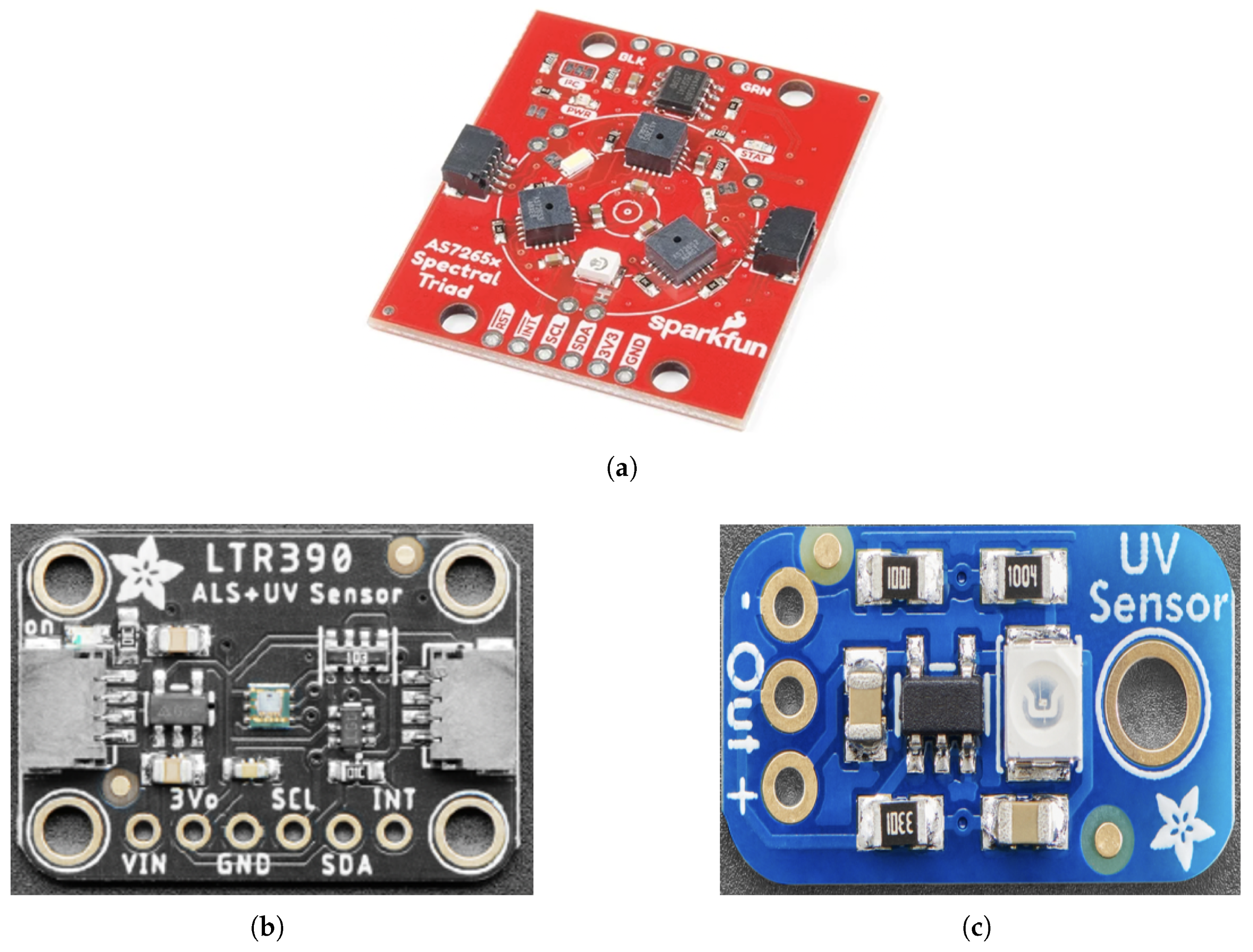
The spectral sensors for the low-cost module were selected based on criteria intended to circumvent the high cost and frequent maintenance requirements typically associated with high-precision instrumentation, thereby being suitable for scalable and dense spatial deployment. These criteria included long-term operational stability, extended sensor lifetime, reduced hardware cost, ease of integration with mobile platforms, and a simplified, robust design. The ensemble includes: an AS7265x Smart Spectral Sensor manufactured by ams Osram [33,34](from SparkFun Electronics, CO, USA), an lLTR390 UV Sensor manufactured by Adafruit Industries [35] (Adafruit Industries, NY, USA), and an Analog GUVA-S12SD UV Sensor also manufactured by Adafruit Industries [36] (Adafruit Industries, NY, USA), at a combined cost of approximately USD 80. Figure 2 depicts the components of the low-cost sensor ensemble.
The constituent sensors were also selected to ensure broad spectral coverage across the solar spectrum. The AS7265x, a smart 18-channel sensor that combines three sensors: the AS72651, the AS72652, and the AS72653, gives raw counts corresponding to the number of photons in each of 18 channels from 400 nm to 1000 nm. The LTR390, one of the few low-cost ultraviolet (UV) sensors available [35], offers UVA sensing with a peak spectral response between 300 nm and 350 nm, and gives unitless digital output values corresponding to both ambient light and UVA intensity. The GUVA-S12SD is capable of detecting the 240 nm to 370 nm range of light, covering the UVB, and most of the UVA spectrum. The output is an analog voltage signal that varies in proportion to the intensity of incident UV radiation, serving as a proxy for the incident UV abundance. The sensors are temporally synced and operate at a temporal frequency of 10 s. In addition to the main body of spectral sensors, the module also hosts a GPS sensor that records the longitude, latitude, and the altitude of the location being observed.
While the low-cost sensor ensemble was curated to span a broad spectral range, and albeit being sufficient for capturing key spectral features relevant to SSI estimation, low-cost sensors are inherently not equivalent in precision to research-grade instruments. Therefore, since the objective is to be able to reproduce NIST-traceable irradiance estimates from these low-cost measurements, the input feature set was augmented with additional key physical determinants of SSI. This included the solar zenith angle, solar azimuth angle, and the surface reflectance. The availability of solar radiation is primarily governed by the Sun’s position relative to the observer [37]. The solar zenith angle and solar azimuth angle determine the position of the Sun in the sky relative to a point on Earth’s surface, and hence play a critical role in the magnitude and distribution of SSI.

2.2. Remote Sensing-Based Surface Reflectance Data

Surface reflectance (SR) is the most fundamental remotely sensed surface parameter, serving as the primary input for a wide range of higher-level land products that depend on solar reflectance characteristics such as vegetation indices, leaf area index, land cover classification, land cover change, and surface albedo [38]. SR is a measure of the fraction of incoming solar radiation that is reflected from the Earth’s surface. It is strongly dependent on the optical properties and structures of the surface. For example, vegetation, soil, water, and snow exhibit distinct reflectance characteristics; snow-covered surfaces typically show much higher reflectance, particularly in the visible spectrum, compared to non-snow-covered land [39], while near-infrared reflectance is specifically sensitive to the vegetation type [40]. Especially in urban areas, SR exhibits significant spatial heterogeneity based on urban geometry surface component variation such as the design, structure, and material of buildings and surfaces in cities (e.g., building shapes, materials, road layouts) [41]. SR is sensitive to changes in land surface caused by both natural and anthropogenic factors [42], and can therefore serve as a proxy for the nature and extent of reflection experienced by downwelling solar radiation at a given location.
As illustrated in Figure 1, surface-reflected radiation forms a significant component of the the total radiative flux at a given point. There could be a radius of surrounding reflectivity that could be affecting and contributing to our SSI measurements, particularly in densely built urban landscapes. Therefore, we augmented the model’s input features with SR data. The data were sourced from the Harmonized Sentinel-2 MSI: MultiSpectral Instrument, Level-2A (SR) product [43]. The MultiSpectral Instrument (MSI) onboard the European Space Agency’s Sentinel-2 satellite constellation is a wide-swath, high-resolution imaging sensor designed for Earth observation across multiple spectral bands. It provides orthorectified, atmospherically corrected SR in 13 spectral bands spanning wavelengths from 442.3 nm to 2202.4 nm, with spatial resolutions of 10 m, 20 m, and 60 m depending on the band. The revisit interval is 5 days. The data are available to query on the Google Earth Engine (GEE) platform. This particular SR product was chosen for several reasons. Firstly, the relatively higher spatial resolution (∼ O ( 10 m ) ) and spectral resolution ensure more accurate and detailed sampling. Secondly, the revisit interval of 5 days is comparatively much smaller than the temporal scale of the inter-day variability in SR [44]. This is especially true in urban settings where surface characteristics remain relatively unchanged over such short intervals, and seasonal trends dominate over daily fluctuations. Finally, its availability on GEE allows spatial and temporal data retrieval to be handled on the cloud, removing the burden of computationally expensive spatial interpolation and large data downloads on the host device. This significantly reduces processing and storage overhead on resource-constrained sensor modules deployed in the field, while still enabling near-real-time integration with local sensor measurements for on-device predictive modeling with edge computing.
We chose SR bands B1, B2, B3, B4, B5, B6, B7, B8, and B8A, which fall within the spectral range of interest for our SSI estimation as inputs to the model.
The Table 1 below lists all the input features used as predictors to the SSI estimation model.

2.3. Reference Instrument

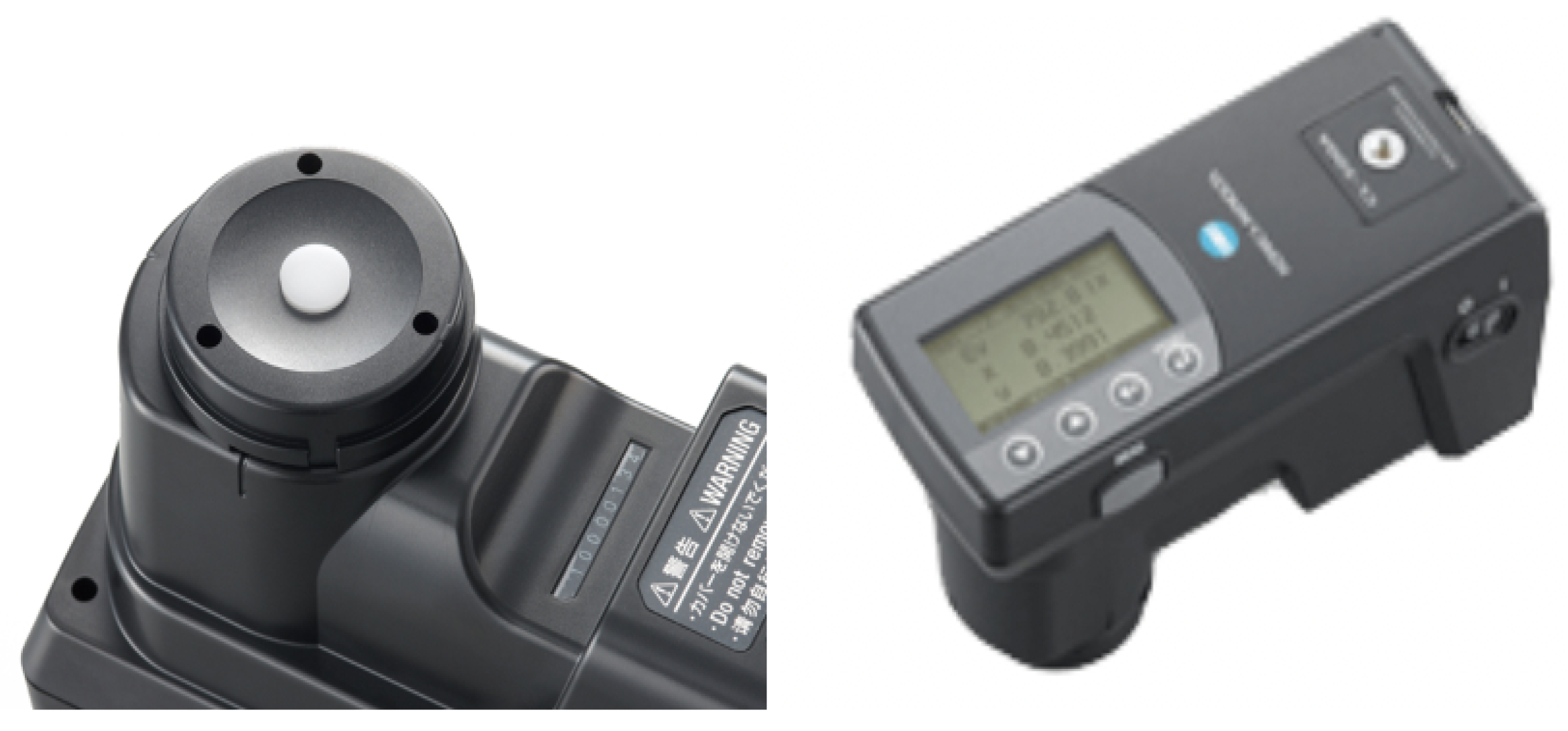
The reference instrument used was an NIST-calibrated Konica Minolta CL-500A spectrophotometer [45] (Konica Minolta Sensing Americas Inc., NJ, USA) with a cost of approximately USD 6000. The Konica Minolta CL-500A (shown in Figure 3) conforms to both DIN and JIS standards. It provides the wavelength-resolved spectral irradiance every 5 s in Wm−2nm−1 at 1 nm resolution from 360 nm to 780 nm in 421 wavelength bins.

2.4. Machine Learning

Machine learning (ML), a branch of artificial intelligence, enables systems to learn from data by example rather than through explicit rule-based programming. It builds empirical models by optimizing patterns derived from sample data, rather than relying on predefined, deterministic algorithms. ML has been effectively applied across diverse domains including in the field of climate physics as an automated method for constructing empirical models directly from data, with notable applications in air quality forecasting [46,47,48,49] and radiative transfer modeling [50]. In the present study, we apply multivariate non-linear nonparametric ML to model wavelength-resolved SSI based on spectral data from a low-cost sensor ensemble and satellite-derived SR, calibrated against target measurements from an NIST-calibrated spectrophotometer.

2.5. Workflow

The reference instrument, capable of providing highly accurate SSI measurements, was co-located and deployed alongside the low-cost sensor module to obtain precise target SSI values for training and validating the machine learning model. The compound module consisting of the low-cost sensor suite and the reference instrument were hosted on the roof of a car and driven in different locations within the Dallas–Fortworth metroplex and the residential cities of Richardson, TX and Carrolton, TX to ensure sampling from varied regions and landscapes at different times during daytime from November 2024 to May 2025. The geographical route of one such data collection trip is given in Figure 4 below. After data collection, in order to integrate the data into a unified dataset for training and validation, all sources were resampled at 10 s intervals and merged based on timestamp alignment. Following this, entries containing NaN values and duplicate samples were removed. The solar zenith and azimuth angles were computed using the Python library pvlib [51] for each individual record. The SR product was queried via the GEE, based on the geographic coordinates (latitude and longitude) and timestamps recorded by the low-cost sensor module. For each coordinate–time pair, the closest Sentinel-2 observation within a 5-day window was identified by minimizing the time difference from the ground-based measurement. Mean surface reflectance values were then extracted for the specific location of observation at 10-m spatial resolution using point-based reduction. The extracted values were subsequently appended to the original dataset, yielding a temporally and spatially aligned data table supplemented with satellite-derived reflectance features. Since satellite-derived measurements can be affected by heavy cloud cover, the Sentinel-2 SR product includes a quality assurance band (QA60) that flags the presence of opaque and cirrus clouds. This QA60 information was used to identify and exclude data instances with potentially unreliable SR values due to cloud obstruction.
Then, the final dataset containing 40,522 individual records was randomly shuffled and split up into two portions, 80% allocated as the training set and the remaining 20% isolated as an independent testing set, on which to assess the performance of the model. We employed the train_test_split function from sklearn.model_selection of the scikit-learn [52] Python library with the shuffle parameter at its default value of True, for this purpose.
The regression algorithm chosen to model SSI was the random forest regressor (RFR) implemented using the scikit-learn [52] library (Version: 1.3.2) in Python (Version 3.8.10). RFR is a flexible regression algorithm with a high degree of accuracy that uses an ensemble of decision trees to make predictions. It combines the output of multiple decision trees to achieve better accuracy and reduce overfitting. RFR can handle large datasets and also supports multi-output regression natively, making it suitable for the present task of predicting wavelength-resolved SSI in 421 spectral bins.
The RFR model was trained on the training set using three-fold cross-validation with the features in Table 1 as inputs to the model and the wavelength-resolved SSI in 421 spectral bins as measured by the reference instrument as the output targets, with hyperparameter optimization using a grid search to build the model with the optimal performance. The hayperparameters tuned during the grid search were as follows: the number of trees (n_estimators), maximum depth of the tree (max_depth), and the number of features to consider when looking for the best split (max_features). The values explored spanned a range of 100 to 500 for n_estimators, 3 to 10 for max_depth, and typical options ’sqrt’, ’log2’, and None for max_features. The final hyperparameter optimized model was trained on the full training set.

3. Results

We developed and trained the ML model to estimate the wavelength-resolved SSI spectrum using only a minimal set of inputs: the spectral responses from an ensemble of low-cost sensors, remotely sensed SR, and easily computable solar geometry parameters, namely, the solar zenith and azimuth angles. The model’s performance was then evaluated on the previously unseen testing set that was held out during training to assess its predictive accuracy and generalization capability. In this section, we present the results.
The scatter plots of estimated vs. true irradiance (i.e., irradiance values observed from the reference instrument) in Figure 5 depict the predictive performance of the model on the training (green) and independent testing (blue) sets across the entire spectrum from 360 nm to 780 nm. The model achieved a co-efficient of determination ( R 2 ) of 0.999 on the training set and an R 2 of 0.997 on the testing set with a significant majority of data points concentrated closer to the 1:1 line. This reflects strong predictive performance, with the high R 2 value on the testing set indicating a good level of generalization to unseen data.
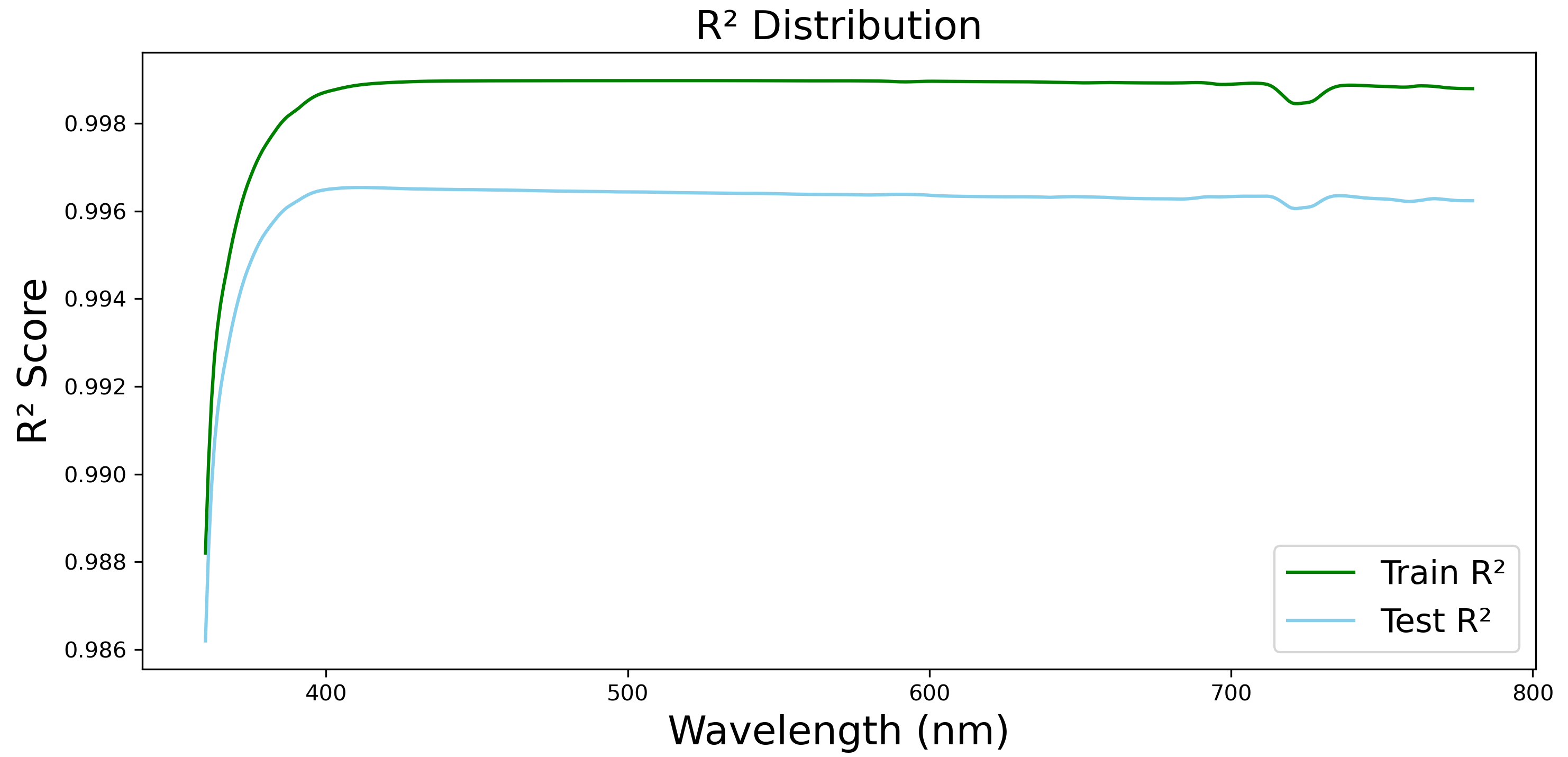
We also evaluated the performance across individual spectral bins. The R 2 values for the performance of the model on the training and testing sets in each individual wavelength bin are given in Figure 6. The model yielded R 2 0.99 across all 421 wavelength bins on the testing set.
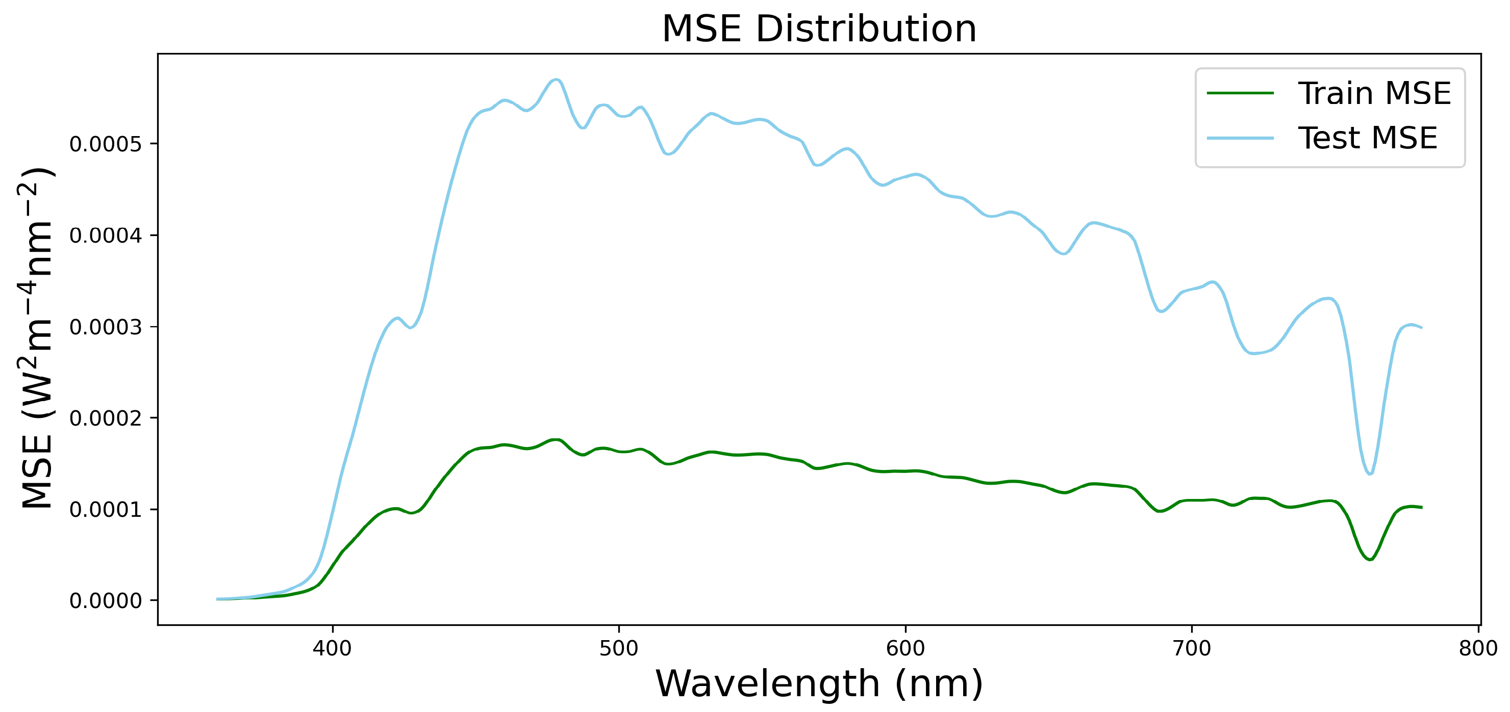
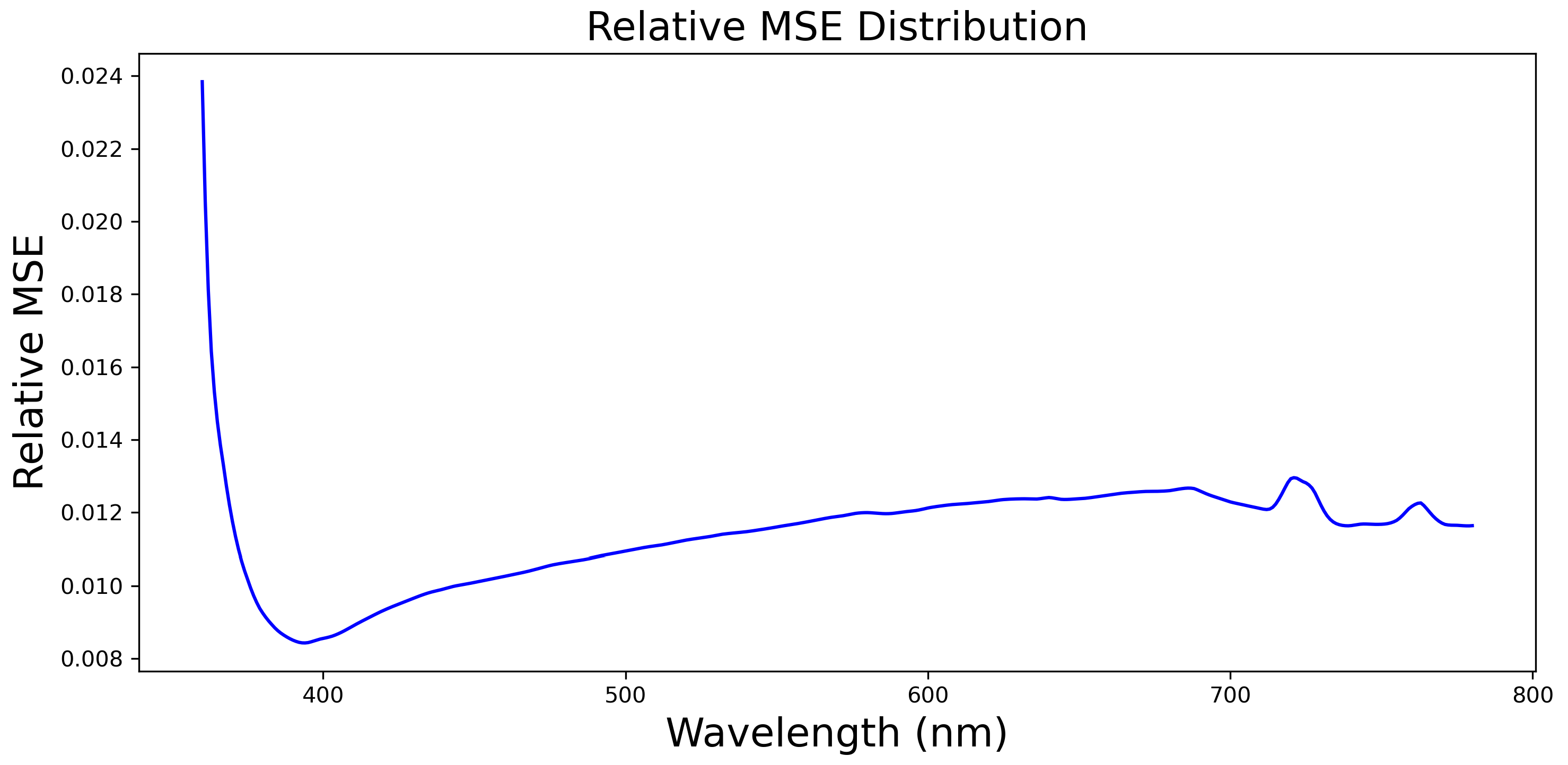
Figure 7 depicts the mean squared error (MSE) for each bin. The MSE across the wavelengths seems to vary in proportion to the magnitude of the values, i.e., the scale of irradiance values within that bin, roughly following the trends in the irradiance variation across the wavelength region. For example, the shortwave bins, particularly in the UV range, are significantly attenuated in the upper atmosphere before reaching the surface, resulting in lower irradiance values in those bins compared to those in the visible region. Therefore, consequently, the MSEs corresponding to these regions are lower in value. In order to gain more context, we further evaluated the relative MSE for each bin. The relative MSE contextualizes the prediction error in relation to the reference scale of the target variable. Figure 8 gives the relative MSEs evaluated on the testing set across the 421 wavelength bins. The relative MSE remains consistently and significantly below unity across all wavelength bins, indicating that the model’s predictive errors are reasonably small in magnitude relative to the corresponding spectral solar irradiance values in each bin. This reflects reliable performance across the entire spectral range.

Application of the Model for Spectral Irradiance Estimation

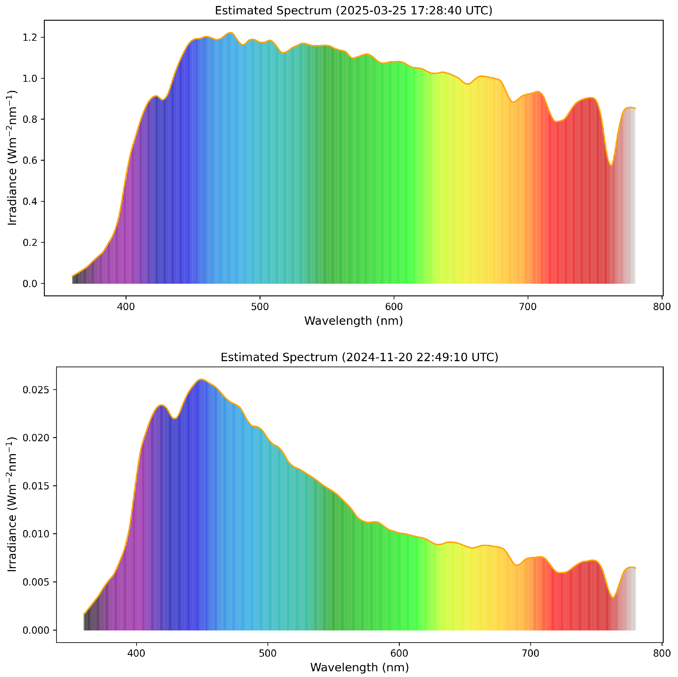
Next, we chose at random a subset of instances from the testing set, and applied our model to estimate the full spectral irradiance from 360 nm to 780 nm using only the readings from the low-cost sensor ensemble, the SR data, and the computed solar zenith and azimuth angles. Figure 9 depicts the estimated irradiance spectra for two representative cases: the top panel corresponding to a day reported as mostly cloudy [53], and the lower panel corresponding to a day reported as relatively clear [54] in the local meteorological records. It is seen how the contrasting weather conditions are reflected in the spectra; the clear-sky spectrum displaying defined peaks in the shorter wavelengths characteristic of a blue sky, whereas the cloudier instance displays a comparatively flattened and diffused shape especially across the blue to red portion of the spectrum. This spectral smoothing arises from enhanced scattering and absorption by cloud water droplets, resulting in a whiter sky appearance. Figure 10 compares the estimated spectra and the corresponding ground-truth spectra measured by the reference instrument. The comparison shows that the ML model effectively captures the overall spectral shape and irradiance values.
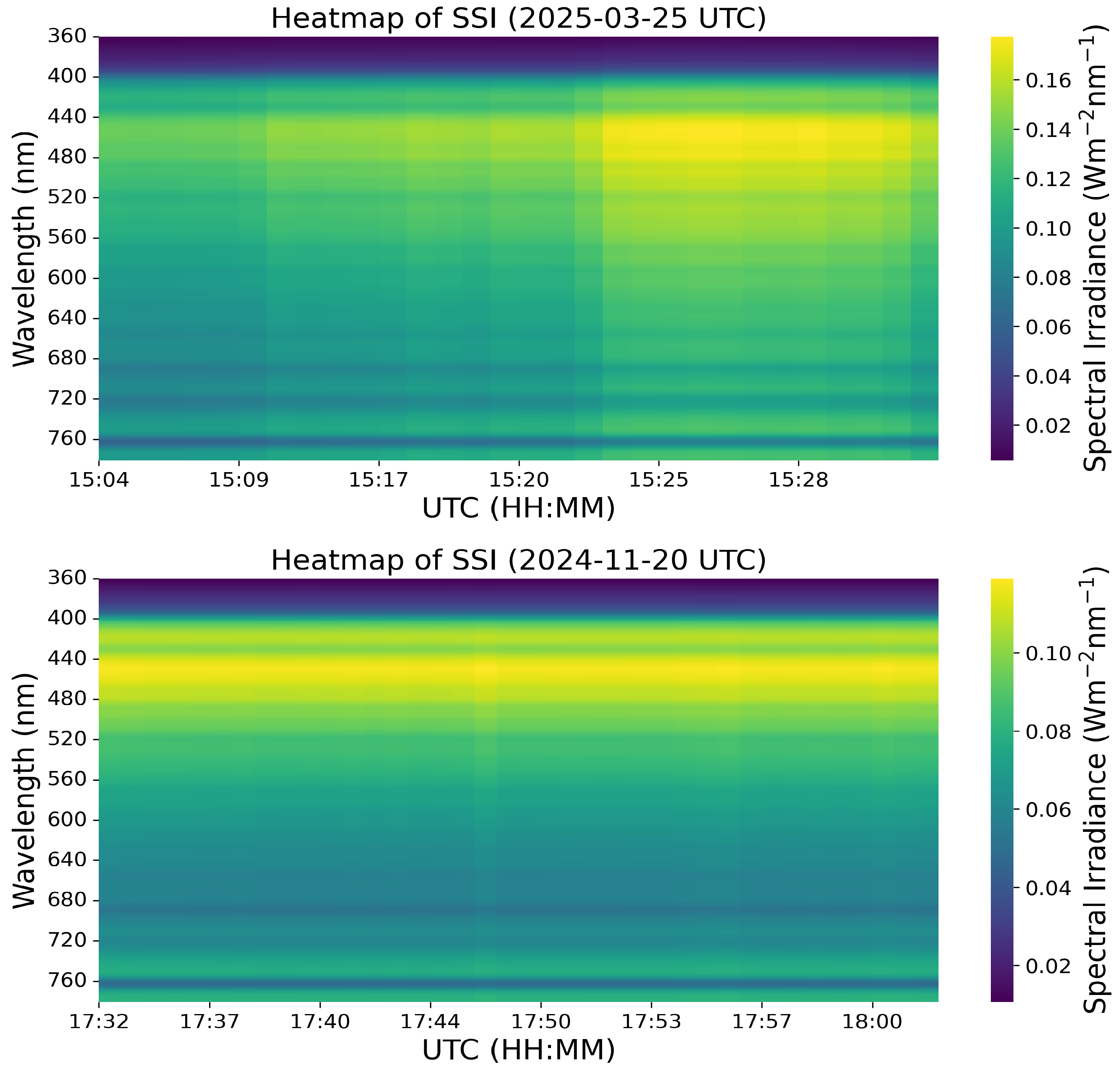
We then selected sets of consecutive time points that were available in the testing set from the same two days to build a time series of SSI and further observe how the respective weather conditions of the day are reflected in the irradiance patterns. Figure 11 depicts the wavelength-resolved SSI estimated by the model across short time intervals on a generally cloudy day (top panel) and a generally clear-sky day (lower panel). The clear-sky weather is clearly apparent in the lower heatmap by the bright, well-defined band corresponding to the blue region of light, sharply contrasting with the adjacent wavelength bands, whereas the top panel corresponding to comparatively cloudier conditions exhibits muted contrast across most of the spectral range. Microscopic water droplets, which form clouds, are excellent sources of Mie scattering [55], which is relatively wavelength-independent, resulting in a more uniform distribution of visible light wavelengths. In contrast, on clearer days, unhindered by clouds, Rayleigh scattering [56] from atmospheric constituents is more prominent. Rayleigh scattering is wavelength-dependent, and most effective at shorter wavelengths, thereby accounting for the peak in the blue-violet region. Figure 12 compares the spectral heatmaps generated by the model with the ground-truth measurements from the reference instrument, using the relative absolute error (RAE). The RAE is defined as:
RAE = | y ^ y | | y |
where y ^ is the model-estimated spectral irradiance value and y is the ground-truth or the corresponding reference instrument reading. In both cases, a substantial majority of estimates fall below approximately 15% RAE. Although the second case includes some points with RAEs around 20%, these represent a smaller proportion of the total. In environmental sensing, an RAE below 20% is often acceptable, considering intrinsic challenges such as sensor noise and atmospheric variability.

4. Extending the SSI Estimation Model to Incorporate Split Conformal Prediction for Principled Uncertainty Quantification

Our proposed approach to quantifying SSI pivots on leveraging ML. ML models inherently involve a certain level of uncertainty. As an extension of this work, to address this, we explored the incorporation of split conformal prediction into our framework to enable the generation of statistically rigorous confidence intervals for our model estimates.
Split conformal prediction [57,58,59] constructs prediction intervals using a hold-out calibration set that is separate from the training data. After training a prediction model on the training set, a nonconformity score, in this case, the absolute error:
R i = | f ( X i ) y i |
where f ( X i ) is the trained ML model applied to the ith calibration record and y i is the true value of the target at the ith instance, is computed for each point in the calibration set. The interval half width δ α is then calculated as the ( 1 α ) ( 1 + 1 n ) th empirical quantile to ensure a coverage level of ( 1 α ) on the calibration set. Prediction intervals for new data are then formed as f ( X n e w ) ± δ α .
To integrate the framework with conformal prediction, we retrained our model, this time splitting the dataset to set aside a calibration set: a total of 20% of the total dataset was isolated as an independent testing set, and the remaining 80% was resplit to allocate 80% as the training set and 20% as the calibration set for the conformal prediction. Then, using the trained model and the calibration set, split conformal prediction as implemented in the Python library Puncc (Predictive uncertainty calibration and conformalization) [57] was applied to evaluate the associated uncertainty of the model. We set α = 0.2 for a coverage corresponding to 80%. Finally, the model was evaluated on the independent testing set and the performance metrics were generated.
Given the substantially large size of our dataset, the additional data split to isolate a calibration set had a negligible impact on the overall model performance. We present below the performance metrics of the model integrated with split conformal prediction: Figure 13 illustrates the model’s predictive performance on both the training set (green) and the independent testing set (blue) across the full spectral range of 360 nm to 780 nm. Figure 14 presents the R 2 for the model’s performance in each individual wavelength bin on both the training and testing sets. Figure 15 shows the MSE per bin, while Figure 16 illustrates the relative MSE values computed on the testing set across all 421 wavelength bins.
The metrics depicted in Figure 13 through Figure 16 are comparable to and closely mirror Figure 5 through Figure 8, demonstrating that the integration of uncertainty estimation can be adopted without compromising the predictive accuracy of the model.
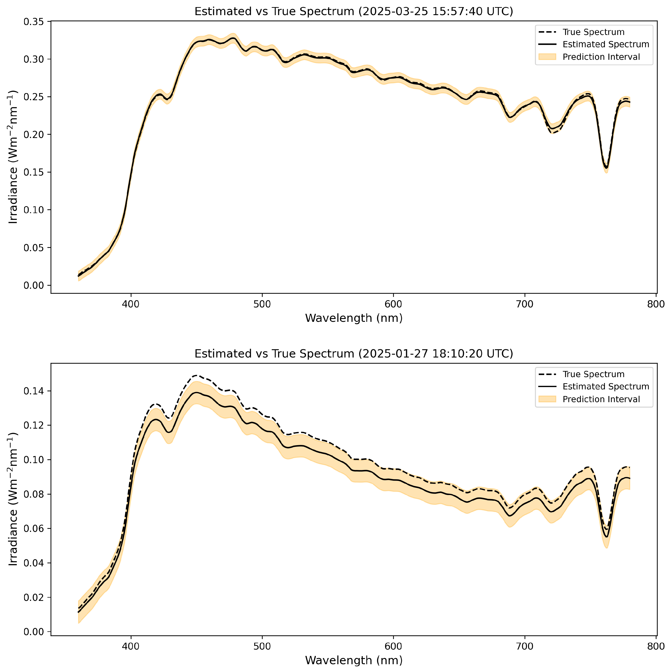
We randomly selected a subset of instances from the testing set and applied the model augmented with split conformal prediction to estimate the full spectral irradiance from 360 nm to 780 nm, along with 80% conformal prediction intervals. Figure 17 presents two examples of the estimated spectral irradiance, each accompanied by 80% conformal prediction intervals and compared against the corresponding ground-truth spectra.
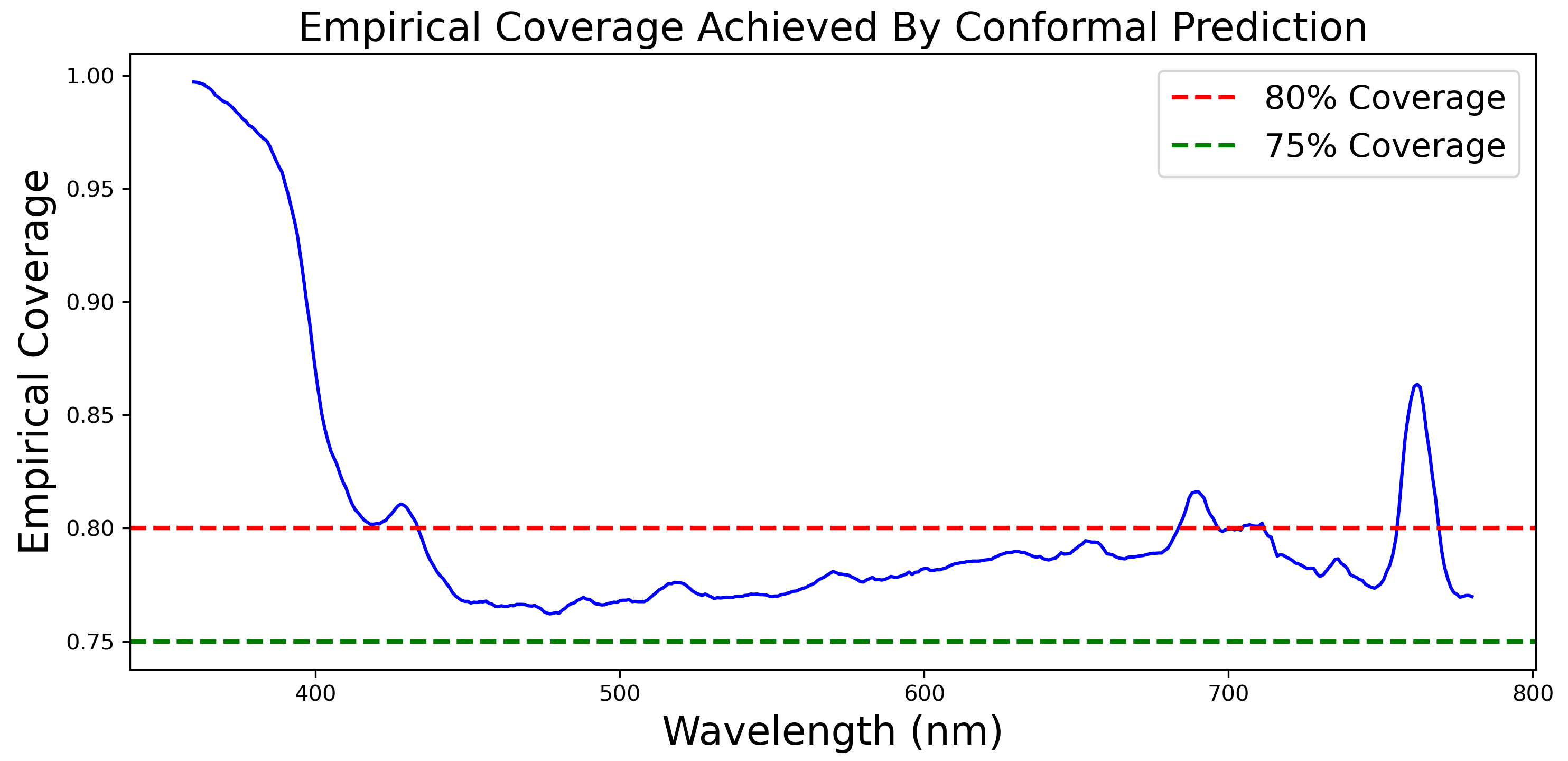
We also evaluated the empirical coverage achieved by the predicted uncertainty on the independent testing set, assessing the percentage of ground-truth values that actually fall within the model’s prediction interval for each wavelength bin. The results are showcased in Figure 18.
The majority of the wavelength bins, particularly in the 450 nm–750 nm region, fall within or acceptably close to the expected 80% coverage level. This indicates that the prediction interval generated from split conformal prediction provides a valid and reliable uncertainty quantification for these regions. However, the shorter wavelength bins (approximately 360 nm–420 nm) exhibit notable over-coverage, with the prediction interval capturing the true values nearly 100% of the time. This can indicate that the prediction interval is excessively wide for these wavelength regions. These shorter wavelengths tend to have weaker irradiance in many terrestrial environments, especially under atmospheric attenuation. As a result, these wavelength bins generally contain irradiance values smaller in magnitude compared to the rest of the spectrum. Therefore the prediction interval generated from split conformal prediction for the model can be disproportionately large relative to the signal strength in these bins. This does not reflect the model’s predictive accuracy (which is measured by metrics such as R 2 and MSE), and solely pertains to the practical usefulness of the predicted uncertainty in these spectral regions. Specifically, overly wide intervals reduce the informativeness in the uncertainty quantification.

5. Societal Relevance and Significance

In this study, we have proposed a machine learning approach that utilizes an ensemble of low-cost sensors together with remote-sensed SR data to accurately estimate wavelength-resolved SSI comparable to observations made by a research grade spectrometer. The model’s performance on the testing data demonstrates its ability to estimate SSI with reasonable accuracy across the wavelength range of 360 nm to 780 nm.
As discussed in Section 1, SSI shows spatiotemporal variability across multiple orders of magnitude, driven by factors such as cloud fields, atmospheric scattering, and absorption by gas molecules, aerosols, and surface elements like vegetation, etc. Studies [23,60] show that the variability in SSI can be on scales as small as seconds or meters. Drawing on a decade of high-resolution SSI data and cloud size distribution modeling to study how cloud size distributions drive the spatiotemporal scales of irradiance variability, ref. [23] demonstrated that fully modeling the variability in SSI requires resolving down to scales as fine as tens of meters. However, achieving this level of spatial resolution using conventional ground-based radiometers is impractical due to cost constraints. Also, in practice, even the most detailed operational weather models run at a resolution of around 1 km [60]. Many remote sensing products providing SSI operate at scales of several kilometers. For example, the satellite-based SSI product Heliosat (SARAH) [26] typically provides data at spatial resolutions corresponding to a 0.05 latitude, longitude grid, and the Copernicus Atmosphere Monitoring Service (CAMS) Radiation Service [24,25] operates on a 0.1 latitude, longitude grid. Therefore, these are inadequate to capture SSI at the required scales. Our approach provides a potential alternative to address this, since due to their affordability, the low-cost sensor modules can be practically deployed at the hyperlocal scale bypassing the cost constraints introduced by conventional spectroradiometers. By hosting the trained model on an edge device and integrating it with satellite-derived SR data, SSI can be estimated using real-time readings from the sensor ensemble alongside the remotely sensed inputs. Since the SR data are available at a temporal frequency of five days, and each sensor module will typically be deployed at a fixed location, this eliminates the need to query SR data for every individual reading. Instead, the SR data can be retrieved once for the specific location and reused until the next satellite revisit.

6. Discussion and Future Directions

In the current study, we have built and validated our framework for SSI estimation based on data collected within the Dallas–Fort Worth climate region, which is humid subtropical with hot summers and generally mild winters [61] and is predominantly urban. This naturally excludes any extensive rural landscapes or heavily snow/ice-covered terrains where phenomena such as snow–cloud confusion [62] become relevant, and where snow cover, in combination with canopy structure, influences reflectance properties in distinct ways [39]. In future work, we aim to expand the data collection across diverse climatic and land use zones to assess the broader applicability of our framework. While the present work showcases the effectiveness of our proposed framework at SSI estimation using the data collected so far from November 2024 to May 2025, since SSI exhibits seasonal variation, the data collection is ongoing, and we intend to incorporate additional data to extend the model’s applicability across the full year.
While we have attempted to curate our low-cost sensor ensemble to include sensors with long-term operational stability, over time, sensors, especially low-cost ones, can experience drift where their measurements slowly become less accurate due to environmental exposure or internal hardware degradation. This can compromise the readings obtained from these, and consequentially the SSI inferred from these readings. Therefore, once the sensor modules are deployed, it is imperative that periodic checks are carried out to ensure reliable performance with ongoing routine calibration and validation. It is also worth noting that the proposed framework for SSI estimation is bound by the capabilities and limitations of the reference instrument used for calibration. While we have utilized an NIST-calibrated Konica Minolta CL-500A conforming to both DIN and JIS standards in order to enable research-grade SSI measurements, it is limited by its range of wavelength measurement, i.e., 360 nm to 780 nm.
While deep learning architectures such as convolutional neural networks are well suited for modeling complex spatial or sequential patterns such as those found in spectral data, they were not explored in the current study. A primary focus was on achieving deployment efficiency on resource-constrained platforms, where tree-based models like RFRs provide a favorable balance between performance and computational cost. They perform well with smaller datasets, whereas neural networks typically require larger amounts of data to achieve similar accuracy [63]. Many CNN architectures require specialized hardware like GPUs, which can be impractical to facilitate on low-cost devices meant for deployment at scale. Tree-based algorithms have also been widely and successfully applied in the literature for estimating environmental parameters from low-cost sensor data and in various remote sensing tasks [64,65]. While not explored within the scope of the present study since the predictive performance of our approach using RFR was found to be sufficiently strong, a quantitative comparison between RFR and deep learning approaches would be a valuable direction for future research.
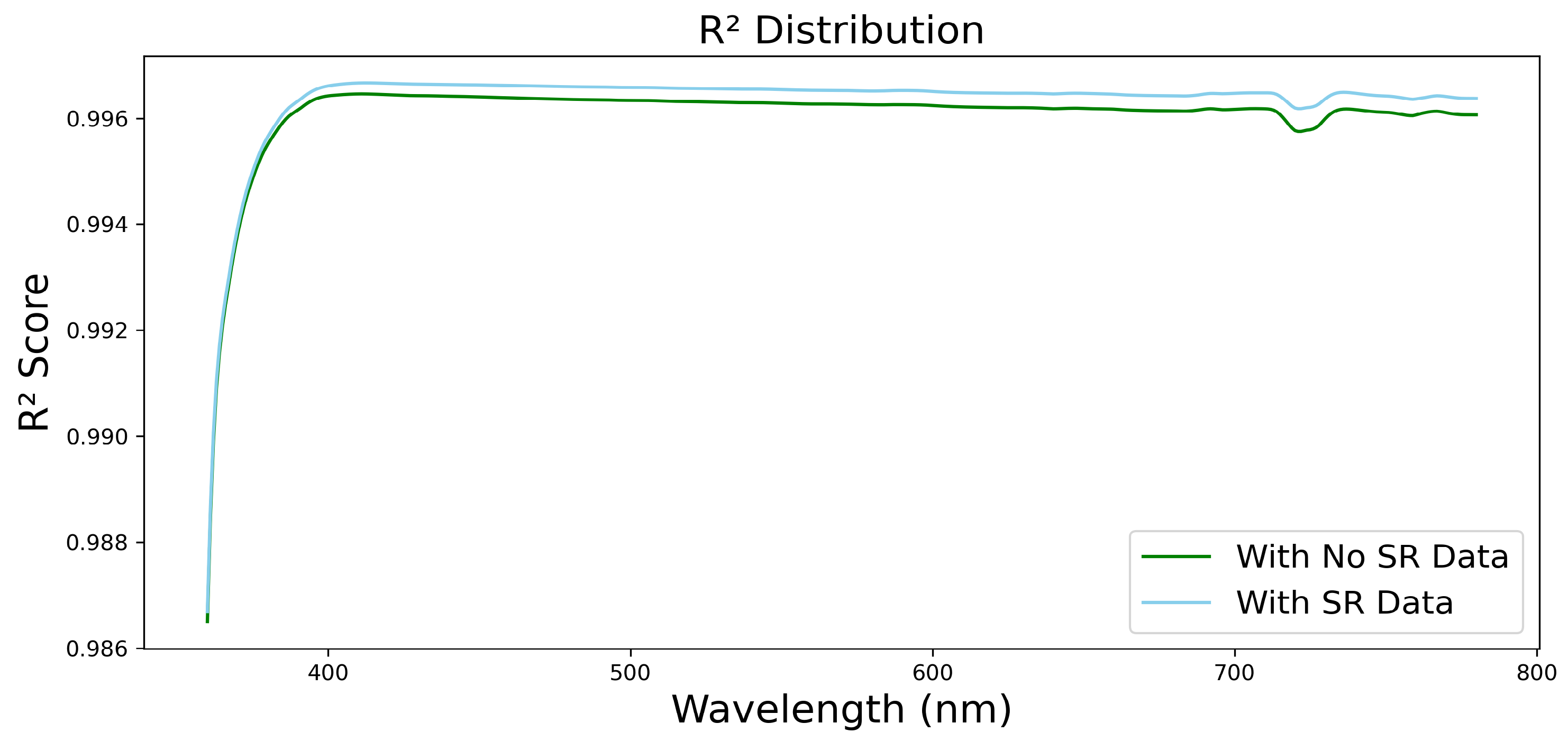
The Sentinel-2 SR product provides reflectance values every five days, captured at a single time during the day. Although SR is a directional quantity influenced by solar illumination geometry, and thus varies diurnally with changes in solar zenith angle, the use of once-daily Sentinel-2 SR data proves effective for predicting SSI at various times of the day, as is apparent from the performance metrics of the model. This is because SR serves as a robust proxy for surface characteristics relevant to irradiance. As detailed in Section 2.2, SR encodes intrinsic land surface properties, such as land cover type, vegetation density, and built environment features, all of which strongly modulate local solar reflectance and, consequently, SSI. Moreover, Sentinel-2 SR observations are typically acquired at consistent local solar times, providing temporal regularity across scenes. Our model includes solar angle parameters, and is trained on a large, diverse dataset spanning a wide range of times, geographic locations, and atmospheric conditions. This diversity enables the model to implicitly learn the stable surface signal embedded in SR. Also, the intra-day variation in SR due to changes in solar geometry is generally small compared to the variation in SSI introduced by dynamic atmospheric conditions such as clouds and aerosols. In fact we evaluated the model’s performance with and without the SR bands as input features. Figure 19 and Figure 20 below show respectively the variation in R2 and MSE evaluated on the testing set across the wavelength range for both approaches. It is evident that incorporating SR leads to improved model performance. This serves as an example of effectively downscaling coarse-temporal-resolution satellite data to derive parameters with high temporal resolution.
While the use of SR as a stable predictor is both logical and empirically validated by the model’s improved performance, it is not without limitations in the operational context. Satellite-derived data can be obstructed and unavailable in heavy, opaque cloud conditions. Since the SR input is available at a 5-day resolution and given that the temporal variability of SR is typically slower than the daily scale, occasional cloudiness on random days is unlikely to affect operation. However, in geographical locations that experience persistent cloud cover over extended periods (e.g., monsoon regions during monsoon seasons), the absence of recent SR observations could hinder the model’s ability to continuously estimate SSI. This constitutes a key limitation in our approach. In such regions, an alternative may be to replace the missing SR instances with monthly averaged values. However, this should be done only after a careful analysis of the temporal variability of SR and its stability over time in the specific region.
We also explored integrating split conformal prediction into our ML model to enable uncertainty quantification. This approach yielded statistically valid and meaningful uncertainty quantification across the majority of the spectral range without compromising predictive accuracy. However, for the lower wavelength bins, the resulting interval could often be disproportionately wide relative to the smaller target values, rendering them less informative. As part of future work, we aim to investigate more adaptive conformal prediction techniques that utilize scaled nonconformity scores, such as locally adaptive conformal regression [66], to improve the calibration of uncertainty estimates across the entire spectral range.

7. Conclusions

We demonstrate that wavelength-resolved surface solar irradiance can be estimated with a high degree of accuracy using machine learning, by combining data from an ensemble of low-cost sensors with remotely sensed surface reflectance inputs. By leveraging affordable, widely deployable sensors integrated with edge computing capabilities, our framework can be put to use to enable fine-grained quantification of surface solar irradiance at high spatial and temporal resolutions, effectively capturing its natural variability for applications in energy and climate research.

Author Contributions

Conceptualization, D.J.L., V.S. and Y.Z.; methodology, V.S. and D.J.L.; software, V.S., L.O.H.W. and Y.Z.; validation, V.S., D.J.L. and L.O.H.W.; formal analysis, V.S.; investigation, V.S.; resources, D.J.L., L.O.H.W., Y.Z., V.S., J.W. and R.P.; data curation, V.S., L.O.H.W.; writing—original draft preparation, V.S.; writing—review and editing, D.J.L. and V.S.; visualization, V.S.; supervision, D.J.L.; project administration, D.J.L.; funding acquisition, D.J.L. All authors have read and agreed to the published version of the manuscript.

Funding

This research was funded by the following grants: The Texas National Security Network Excellence Fund award for Environmental Sensing Security Sentinels; the SOFWERX award for Machine Learning for Robotic Teams and NSF Award OAC-2115094; support from the University of Texas at Dallas Office of Sponsored Programs, Dean of Natural Sciences and Mathematics, and Chair of the Physics Department is gratefully acknowledged; TRECIS CC* Cyberteam (NSF #2019135); NSF OAC-2115094 Award; and EPA P3 grant number 84057001-0.

Institutional Review Board Statement

Not applicable.

Informed Consent Statement

Not applicable.

Data Availability Statement

The data used for the training and testing of the model are publicly available at https://github.com/mi3nts/SSI_Estimation, accessed on 30 July 2025.

Conflicts of Interest

The authors declare no conflicts of interest.

Abbreviations

The following abbreviations are used in this manuscript:
SSISurface solar irradiance
UVUltraviolet
SRSurface reflectance
GEEGoogle Earth Engine
MLMachine learning
RFRRandom forest regressor
R2Coefficient of determination
MSEMean squared error
RAERelative absolute error

References

  1. Gessler, A.; Bugmann, H.; Bigler, C.; Edwards, P.; Guistina, C.D.; Kueffer, C.; Roy, J.; Resco de Dios, V. Light as a Source of Information in Ecosystems; American Association for the Advancement of Science: Washington, DC, USA, 2017. [Google Scholar]
  2. Mellouki, A.; Wallington, T.; Chen, J. Atmospheric chemistry of oxygenated volatile organic compounds: Impacts on air quality and climate. Chem. Rev. 2015, 115, 3984–4014. [Google Scholar] [CrossRef]
  3. Sillman, S. The relation between ozone, NOx and hydrocarbons in urban and polluted rural environments. Atmos. Environ. 1999, 33, 1821–1845. [Google Scholar] [CrossRef]
  4. Levy, H., II. Photochemistry of the lower troposphere. Planet. Space Sci. 1972, 20, 919–935. [Google Scholar] [CrossRef]
  5. Zhang, Y.; Wijeratne, L.O.H.; Talebi, S.; Lary, D.J. Machine learning for light sensor calibration. Sensors 2021, 21, 6259. [Google Scholar] [CrossRef] [PubMed]
  6. Hartmann, D.L. Atmospheric radiative transfer and climate. Glob. Phys. Climatol. 2016, 2016, 49–94. [Google Scholar]
  7. Buehler, S.A.; Mendrok, J.; Eriksson, P.; Perrin, A.; Larsson, R.; Lemke, O. ARTS, the atmospheric radiative transfer simulator–version 2.2. Geosci. Model Dev. 2018, 11, 1537–1556. [Google Scholar] [CrossRef]
  8. Lary, D.; Pyle, J. Diffuse radiation, twilight, and photochemistry—I. J. Atmos. Chem. 1991, 13, 373–392. [Google Scholar] [CrossRef]
  9. Lary, D.J.; Alavi, A.H.; Gandomi, A.H.; Walker, A.L. Machine learning in geosciences and remote sensing. Geosci. Front. 2016, 7, 3–10. [Google Scholar] [CrossRef]
  10. Chen, L.; Yan, G.; Wang, T.; Ren, H.; Calbó, J.; Zhao, J.; McKenzie, R. Estimation of surface shortwave radiation components under all sky conditions: Modeling and sensitivity analysis. Remote Sens. Environ. 2012, 123, 457–469. [Google Scholar] [CrossRef]
  11. Lohmann, G.M.; Monahan, A.H.; Heinemann, D. Local short-term variability in solar irradiance. Atmos. Chem. Phys. 2016, 16, 6365–6379. [Google Scholar] [CrossRef]
  12. Solar Power Europe. Global Market Outlook for Solar Power 2015–2019. 2015. Available online: http://www.solarpowereurope.org/ (accessed on 7 September 2015).
  13. Stetz, T.; von Appen, J.; Niedermeyer, F.; Scheibner, G.; Sikora, R.; Braun, M. Twilight of the grids: The impact of distributed solar on Germany?s energy transition. IEEE Power Energy Mag. 2015, 13, 50–61. [Google Scholar] [CrossRef]
  14. Buizer, J. Air quality. In Impacts, Risks, and Adaptation in the United States: Fourth National Climate Assessment, Volume II; U.S. Global Change Research Program: Washington, DC, USA, 2018; Chapter 13; p. 516. [Google Scholar]
  15. Sanchez-Lorenzo, A.; Wild, M.; Brunetti, M.; Guijarro, J.A.; Hakuba, M.Z.; Calbó, J.; Mystakidis, S.; Bartok, B. Reassessment and update of long-term trends in downward surface shortwave radiation over Europe (1939–2012). J. Geophys. Res. Atmos. 2015, 120, 9555–9569. [Google Scholar] [CrossRef]
  16. Jang, J.C.; Sohn, E.H.; Park, K.H. Estimating hourly surface solar irradiance from GK2A/AMI data using machine learning approach around Korea. Remote Sens. 2022, 14, 1840. [Google Scholar] [CrossRef]
  17. Henzing, J.; Knap, W.; Stammes, P.; Apituley, A.; Bergwerff, J.; Swart, D.; Kos, G.; Ten Brink, H. Effect of aerosols on the downward shortwave irradiances at the surface: Measurements versus calculations with MODTRAN4. 1. J. Geophys. Res. Atmos. 2004, 109, D14204. [Google Scholar] [CrossRef]
  18. Jacovides, C.P.; Steven, M.D.; Asimakopoulos, D.N. Spectral solar irradiance and some optical properties for various polluted atmospheres. Sol. Energy 2000, 69, 215–227. [Google Scholar] [CrossRef]
  19. Latha, K.M.; Badarinath, K. Spectral solar attenuation due to aerosol loading over an urban area in India. Atmos. Res. 2005, 75, 257–266. [Google Scholar] [CrossRef]
  20. Nevins, M.G.; Apell, J.N. Emerging investigator series: Quantifying the impact of cloud cover on solar irradiance and environmental photodegradation. Environ. Sci. Processes Impacts 2021, 23, 1884–1892. [Google Scholar] [CrossRef]
  21. Gueymard, C.A. Cloud and albedo enhancement impacts on solar irradiance using high-frequency measurements from thermopile and photodiode radiometers. Part 1: Impacts on global horizontal irradiance. Sol. Energy 2017, 153, 755–765. [Google Scholar] [CrossRef]
  22. Yordanov, G.H. A study of extreme overirradiance events for solar energy applications using NASA’s I3RC Monte Carlo radiative transfer model. Sol. Energy 2015, 122, 954–965. [Google Scholar] [CrossRef]
  23. Mol, W.B.; van Stratum, B.J.; Knap, W.H.; van Heerwaarden, C.C. Reconciling observations of solar irradiance variability with cloud size distributions. J. Geophys. Res. Atmos. 2023, 128, e2022JD037894. [Google Scholar] [CrossRef]
  24. Copernicus Atmosphere Monitoring Service. CAMS Solar Radiation Time-Series. Copernicus Atmosphere Monitoring Service (CAMS) Atmosphere Data Store. 2020. Available online: https://ads.atmosphere.copernicus.eu/datasets/cams-solar-radiation-timeseries?tab=overview (accessed on 12 June 2025).
  25. Copernicus Atmosphere Monitoring Service. CAMS Gridded Solar Radiation. Copernicus Atmosphere Monitoring Service (CAMS) Atmosphere Data Store, 2022. Available online: https://ads.atmosphere.copernicus.eu/ (accessed on 12 June 2025).
  26. Pfeifroth, U.; Kothe, S.; Drücke, J.; Trentmann, J.; Schröder, M.; Selbach, N.; Hollmann, R. Surface Radiation Data Set—Heliosat (SARAH), 3rd ed.; Satellite Application Facility on Climate Monitoring (CM SAF): Offenbach, Germany, 2023. [Google Scholar] [CrossRef]
  27. GOES-R Algorithm Working Group and GOES-R Program Office. NOAA GOES-R Series Advanced Baseline Imager (ABI) Level 2 Downward Shortwave Radiation: Surface; NOAA National Centers for Environmental Information: Asheville, NC, USA, 2017. Available online: https://www.ncei.noaa.gov/access/metadata/landing-page/bin/iso?id=gov.noaa.ncdc:C01524 (accessed on 12 June 2025).
  28. Boudjella, M.Y.; Belbachir, A.H.; Dib, S.A.A.; Meftah, M. Calculation of surface spectral irradiance using the Geant4 Monte Carlo toolkit. J. Atmos. Sol.-Terr. Phys. 2023, 248, 106077. [Google Scholar] [CrossRef]
  29. Anderson, T.L.; Charlson, R.J.; Winker, D.M.; Ogren, J.A.; Holmén, K. Mesoscale variations of tropospheric aerosols. J. Atmos. Sci. 2003, 60, 119–136. [Google Scholar] [CrossRef]
  30. Breitkreuz, H.; Schroedter-Homscheidt, M.; Holzer-Popp, T.; Dech, S. Short-range direct and diffuse irradiance forecasts for solar energy applications based on aerosol chemical transport and numerical weather modeling. J. Appl. Meteorol. Climatol. 2009, 48, 1766–1779. [Google Scholar] [CrossRef]
  31. Kinne, S.; Schulz, M.; Textor, C.; Guibert, S.; Balkanski, Y.; Bauer, S.E.; Berntsen, T.; Berglen, T.F.; Boucher, O.; Chin, M.; et al. An AeroCom initial assessment—Optical properties in aerosol component modules of global models. Atmos. Chem. Phys. Discuss. 2005, 5, 8285–8330. [Google Scholar] [CrossRef]
  32. Schmidt, G.A.; Ruedy, R.; Hansen, J.E.; Aleinov, I.; Bell, N.; Bauer, M.; Bauer, S.; Cairns, B.; Canuto, V.; Cheng, Y.; et al. Present-day atmospheric simulations using GISS ModelE: Comparison to in situ, satellite, and reanalysis data. J. Clim. 2006, 19, 153–192. [Google Scholar] [CrossRef]
  33. ams OSRAM. ams AS7265x Smart Spectral Sensor. Available online: https://ams-osram.com/products/sensor-solutions/ambient-light-color-spectral-proximity-sensors/ams-as7265x-smart-spectral-sensor (accessed on 16 June 2025).
  34. SparkFun. SparkFun Triad Spectroscopy Sensor—AS7265x (Qwiic). Available online: https://www.sparkfun.com/sparkfun-triad-spectroscopy-sensor-as7265x-qwiic.html (accessed on 16 June 2025).
  35. Adafruit. Adafruit LTR390 UV Light Sensor—STEMMA QT/Qwiic. Available online: https://www.adafruit.com/product/4831 (accessed on 16 June 2025).
  36. Adafruit. Analog UV Light Sensor Breakout - GUVA-S12SD. Available online: https://www.adafruit.com/product/1918?srsltid=AfmBOopzuG3d4hTw_7uGepxUQev8_2LAAsoi3K-3PGq8Gp_u80qEr6yj (accessed on 16 June 2025).
  37. Perez-Astudillo, D.; Bachour, D.; Martin-Pomares, L. Effect of Solar Position Calculations on Filtering and Analysis of Solar Radiation Measurements. In Proceedings of the ISES EuroSun 2018 Conference—12th International Conference on Solar Energy for Buildings and Industry, Rapperswil, Switzerland, 10–13 September 2018. [Google Scholar]
  38. NOAA STAR Land Team. Surface Reflectance Product Overview, 2024. Available online: https://www.star.nesdis.noaa.gov/smcd/emb/land/index.php?product=SR (accessed on 10 June 2025).
  39. Burakowski, E.A.; Ollinger, S.V.; Lepine, L.; Schaaf, C.B.; Wang, Z.; Dibb, J.E.; Hollinger, D.Y.; Kim, J.; Erb, A.; Martin, M. Spatial scaling of reflectance and surface albedo over a mixed-use, temperate forest landscape during snow-covered periods. Remote Sens. Environ. 2015, 158, 465–477. [Google Scholar] [CrossRef]
  40. Almalki, R.; Khaki, M.; Saco, P.M.; Rodriguez, J.F. Monitoring and mapping vegetation cover changes in arid and semi-arid areas using remote sensing technology: A review. Remote Sens. 2022, 14, 5143. [Google Scholar] [CrossRef]
  41. Wu, H.; Huang, B.; Zheng, Z.; Ma, Z.; Zeng, Y. Spatial Heterogeneity and Temporal Variation in Urban Surface Albedo Detected by High-Resolution Satellite Data. Remote Sens. 2022, 14, 6166. [Google Scholar] [CrossRef]
  42. Lee, K.S.; Lee, E.; Jin, D.; Seong, N.H.; Jung, D.; Sim, S.; Han, K.S. Retrieval and uncertainty analysis of land surface reflectance using a geostationary ocean color imager. Remote Sens. 2022, 14, 360. [Google Scholar] [CrossRef]
  43. European Union/ESA/Copernicus. Sentinel-2 MSI: MultiSpectral Instrument, Level-2A Surface Reflectance (SR). Available online: https://developers.google.com/earth-engine/datasets/catalog/COPERNICUS_S2_SR (accessed on 10 June 2025).
  44. Park, S.S.; Yu, J.E.; Lim, H.; Lee, Y.G. Temporal variation of surface reflectance and cloud fraction used to identify background aerosol retrieval information over East Asia. Atmos. Environ. 2023, 309, 119916. [Google Scholar] [CrossRef]
  45. KONICA MINOLTA. CL-500A Illuminance Spectrophotometer. Available online: https://sensing.konicaminolta.us/us/products/cl-500a-illuminance-spectrophotometer/ (accessed on 16 June 2025).
  46. Shin, S.; Baek, K.; So, H. Rapid monitoring of indoor air quality for efficient HVAC systems using fully convolutional network deep learning model. Build. Environ. 2023, 234, 110191. [Google Scholar] [CrossRef]
  47. Ravindiran, G.; Hayder, G.; Kanagarathinam, K.; Alagumalai, A.; Sonne, C. Air quality prediction by machine learning models: A predictive study on the indian coastal city of Visakhapatnam. Chemosphere 2023, 338, 139518. [Google Scholar] [CrossRef]
  48. Wang, S.; McGibbon, J.; Zhang, Y. Predicting high-resolution air quality using machine learning: Integration of large eddy simulation and urban morphology data. Environ. Pollut. 2024, 344, 123371. [Google Scholar] [CrossRef] [PubMed]
  49. Karthick, K.; Aruna, S.K.; Dharmaprakash, R.; Ravindiran, G. Integrating machine learning techniques for Air Quality Index forecasting and insights from pollutant-meteorological dynamics in sustainable urban environments. Earth Sci. Inform. 2024, 17, 3733–3748. [Google Scholar]
  50. Su, M.; Liu, C.; Di, D.; Le, T.; Sun, Y.; Li, J.; Lu, F.; Zhang, P.; Sohn, B.J. A multi-domain compression radiative transfer model for the Fengyun-4 Geosynchronous Interferometric Infrared Sounder (GIIRS). Adv. Atmos. Sci. 2023, 40, 1844–1858. [Google Scholar] [CrossRef]
  51. Anderson, K.S.; Hansen, C.W.; Holmgren, W.F.; Jensen, A.R.; Mikofski, M.A.; Driesse, A. pvlib python: 2023 project update. J. Open Source Softw. 2023, 8, 5994. [Google Scholar] [CrossRef]
  52. Pedregosa, F.; Varoquaux, G.; Gramfort, A.; Michel, V.; Thirion, B.; Grisel, O.; Blondel, M.; Prettenhofer, P.; Weiss, R.; Dubourg, V.; et al. Scikit-learn: Machine Learning in Python. J. Mach. Learn. Res. 2011, 12, 2825–2830. [Google Scholar]
  53. NBCDFW. March 25 Spring Storms Bring Hail to North Texas, 2025. Available online: https://www.nbcdfw.com/weather/weather-connection/march-25-spring-storms-hail/3800690/ (accessed on 25 June 2025).
  54. WeatherSpark. Historical Weather in November 2024 in Richardson, Texas, United States, 2024. Available online: https://weatherspark.com/h/m/8846/2024/11/Historical-Weather-in-November-2024-in-Richardson-Texas-United-States (accessed on 24 June 2025).
  55. Mie, G. Beiträge zur Optik trüber Medien, speziell kolloidaler Metallösungen. Ann. Phys. 1908, 330, 377–445. [Google Scholar] [CrossRef]
  56. Rayleigh, J.W.S.B. On the Scattering of Light by Small Particles; Taylor & Francis: Abingdon, UK, 1871. [Google Scholar]
  57. Mendil, M.; Mossina, L.; Vigouroux, D. PUNCC: A Python Library for Predictive Uncertainty Calibration and Conformalization. In Proceedings of the Conformal and Probabilistic Prediction with Applications. PMLR, Limassol, Cyprus, 13–15 September 2023; pp. 582–601. [Google Scholar]
  58. Papadopoulos, H.; Proedrou, K.; Vovk, V.; Gammerman, A. Inductive confidence machines for regression. In Proceedings of the Machine Learning: ECML 2002: 13th European Conference on Machine Learning, Helsinki, Finland, 19–23 August 2002; Proceedings 13. Springer: Berlin/Heidelberg, Germany, 2002; pp. 345–356. [Google Scholar]
  59. Lei, J.; G’Sell, M.; Rinaldo, A.; Tibshirani, R.J.; Wasserman, L. Distribution-free predictive inference for regression. J. Am. Stat. Assoc. 2018, 113, 1094–1111. [Google Scholar] [CrossRef]
  60. Mol, W.; Heusinkveld, B.; Mangan, M.R.; Hartogensis, O.; Veerman, M.; van Heerwaarden, C. Observed patterns of surface solar irradiance under cloudy and clear-sky conditions. Q. J. R. Meteorol. Soc. 2024, 150, 2338–2363. [Google Scholar] [CrossRef]
  61. The National Weather Service (NWS). Dallas/Fort Worth Climate Narrative. Available online: https://www.weather.gov/fwd/dfw_narrative (accessed on 29 July 2025).
  62. Wang, X.; Han, C.; Ouyang, Z.; Chen, S.; Guo, H.; Wang, J.; Hao, X. Cloud–snow confusion with MODIS snow products in boreal forest regions. Remote Sens. 2022, 14, 1372. [Google Scholar] [CrossRef]
  63. Roßbach, P. Neural networks vs. random forests–does it always have to be deep learning. Ger. Frankf. Sch. Financ. Manag. 2018, 1–8. Available online: https://api.semanticscholar.org/CorpusID:221088499 (accessed on 5 August 2025).
  64. Wijeratne, L.O.; Kiv, D.R.; Aker, A.R.; Talebi, S.; Lary, D.J. Using machine learning for the calibration of airborne particulate sensors. Sensors 2019, 20, 99. [Google Scholar] [CrossRef]
  65. Waczak, J.; Aker, A.; Wijeratne, L.O.; Talebi, S.; Fernando, A.; Dewage, P.M.; Iqbal, M.; Lary, M.; Schaefer, D.; Lary, D.J. Characterizing water composition with an autonomous robotic team employing comprehensive in situ sensing, hyperspectral imaging, machine learning, and conformal prediction. Remote Sens. 2024, 16, 996. [Google Scholar] [CrossRef]
  66. Papadopoulos, H.; Gammerman, A.; Vovk, V. Normalized nonconformity measures for regression conformal prediction. In Proceedings of the IASTED International Conference on Artificial Intelligence and Applications (AIA 2008), Innsbruck, Austria, 11–13 February 2008; pp. 64–69. [Google Scholar]
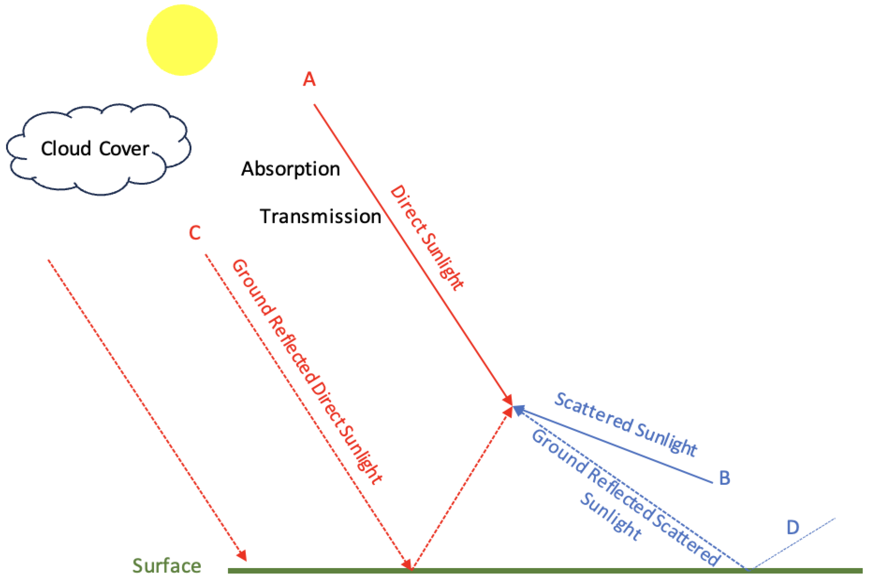
Figure 1. The radiation incident on any volume element of the atmosphere has four contributions: (A) The direct solar flux, (B) the diffuse (scattered) flux incident from all directions, (C) the ground reflection of the direct solar flux, and (D) the ground reflection of the diffuse flux.
Remotesensing 17 02753 g001
Figure 2. Ensemble of low cost sensors. (a) AS7265x Smart Spectral Sensor. Source: [34]. (b) LTR390 UV Light Sensor. Source: [35]. (c) GUVA-S12SD UV Sensor. Source: [36].
Remotesensing 17 02753 g002
Figure 3. The Konica Minolta CL-500A Spectrophotometer. Source: [45].
Remotesensing 17 02753 g003
Figure 4. The geographical route of a data collection trip taken on 2025-05-24. The red pointers indicate the route taken.
Remotesensing 17 02753 g004
Figure 5. Scatter diagram comparing the SSI measurements from the reference instrument on the x-axis against the SSI estimates from the ML model on the y-axis for the whole spectrum from 360 nm to 780 nm.
Remotesensing 17 02753 g005
Figure 6. R 2 values on each of the 421 spectral bins evaluated on the training and testing sets.
Remotesensing 17 02753 g006
Figure 7. MSE values on each of the 421 spectral bins evaluated on the training and testing sets.
Remotesensing 17 02753 g007
Figure 8. Relative MSE values across the 421 spectral bins evaluated on the test set.
Remotesensing 17 02753 g008
Figure 9. Irradiance spectra estimated using the model. The top panel corresponds to a cloudy day and the lower panel corresponds to a clear-sky day.
Remotesensing 17 02753 g009
Figure 10. Irradiance spectrum estimated using the model compared with the ground-truth spectra measured by the reference instrument. The top panel corresponds to a cloudy day and the lower panel corresponds to a clear-sky day.
Remotesensing 17 02753 g010
Figure 11. Wavelength-resolved SSI estimated by the model for brief intervals of time. The top panel corresponds to a cloudy day and the lower panel corresponds to a clear-sky day.
Remotesensing 17 02753 g011
Figure 12. RAE of the estimated spectra compared to observations by the reference instrument.
Remotesensing 17 02753 g012
Figure 13. Scatter diagram comparing the SSI measurements from the reference instrument on the x-axis against the SSI estimates from the ML model on the y-axis for the whole spectrum from 360 nm to 780 nm after incorporating conformal prediction.
Remotesensing 17 02753 g013
Figure 14. R 2 values on each of the 421 spectral bins evaluated on the training and testing sets after incorporating conformal prediction.
Remotesensing 17 02753 g014
Figure 15. MSE values on each of the 421 spectral bins evaluated on the training and testing sets after incorporating conformal prediction.
Remotesensing 17 02753 g015
Figure 16. Relative MSE values across the 421 spectral bins evaluated on the test set after incorporating conformal prediction.
Remotesensing 17 02753 g016
Figure 17. Model-estimated spectra at selected time points, shown with 80% confidence intervals and compared against ground-truth spectra.
Remotesensing 17 02753 g017
Figure 18. Empirical coverage.
Remotesensing 17 02753 g018
Figure 19. R 2 values on each of the 421 spectral bins evaluated on the testing set for the model with SR data vs. with no SR data.
Remotesensing 17 02753 g019
Figure 20. MSE values on each of the 421 spectral bins evaluated on the testing set for the model with SR data vs. with no SR data.
Remotesensing 17 02753 g020
Table 1. Features used as predictors to the SSI estimation model.
FeatureUnitSource
Channel 410 nmCountsAS7265X
Channel 435 nmCounts
Channel 460 nmCounts
Channel 485 nmCounts
Channel 510 nmCounts
Channel 535 nmCounts
Channel 560 nmCounts
Channel 585 nmCounts
Channel 610 nmCounts
Channel 645 nmCounts
Channel 680 nmCounts
Channel 705 nmCounts
Channel 730 nmCounts
Channel 760 nmCounts
Channel 810 nmCounts
Channel 860 nmCounts
Channel 900 nmCounts
Channel 940 nmCounts
Ambient Light
Level Reading
UnitlessLTR390
UVA Level ReadingUnitless
UV Level ProxiesVoltGUVA-S12SD
Solar Zenith AngleDegreesCalculated
Solar Azimuth AngleDegrees
Sentinel-2 Surface Reflectance (Spectral Bands B1, B2, B3, B4, B5, B6, B7, B8, B8A)UnitlessHarmonized Sentinel-2 MSI: MultiSpectral Instrument, Level-2A
(SR) Product
Disclaimer/Publisher’s Note: The statements, opinions and data contained in all publications are solely those of the individual author(s) and contributor(s) and not of MDPI and/or the editor(s). MDPI and/or the editor(s) disclaim responsibility for any injury to people or property resulting from any ideas, methods, instructions or products referred to in the content.