Application of SAR to Delineate Peatland from Other Land Cover and Assess Relative Condition in Relation to Surface Moisture

Abstract

Peatland is a difficult landscape to map due to its challenging conditions. Remote sensing lends itself to mapping efforts, but can be hampered by common weather conditions in peatland locations. Sentinel-1 Synthetic Aperture Radar technology penetrates prevalent cloud cover. Techniques used to detect water surfaces using Sentinel-1 backscatter intensity have been applied in this study to delineate peatland land cover. This application was then extended with the aim of identifying the relative conditions of peatland within an area of interest. A peatland study site was selected at Winter Hill, near Bolton in Lancashire, UK, where a nationally significant wildfire occurred in 2018. Sentinel-1 imagery captured in the winter after the wildfire quite accurately reflected the fire damage extent. From further examination, it was found that in frozen conditions there are significant statistical differences between peatland surfaces and visually similar land cover, such as fields used for livestock grazing. Using the inter-quartile range of land cover samples to identify suitable backscatter thresholds, a surface map was produced depicting peatland of varying conditions and other land cover categories. This was compared with field visit photographic records to ascertain accuracy of representation. Further analysis detected correlation between backscatter and temperature for peatland surfaces that was not evident for other land cover classes. Steeper terrain can though affect this relationship. Conversely, no significant connection could be found in areas where surface water is most likely to be retained. Aggregating Sentinel-1 backscatter according to sub-catchment zones presented the potential to further delineate by condition within a peatland land cover sample. Therefore, the use of Sentinel-1 imagery in frozen conditions in context with terrain and sub-catchment level hydrological zoning provides the opportunity to aid environmental monitoring by delineating peatland from other land cover, identifying climate-change effects such as wildfires and assessing relative condition at scale.

1. Introduction

The motivation for this research was borne from the benefits that Synthetic Aperture Radar (SAR) satellite data, such as the Copernicus Sentinel-1 programme, can bring in detecting water inundation [1]. The ability of SAR to identify and delineate surfaces with a higher presence of moisture offers the potential to classify wet, healthy and dry, degraded peatland. C-Band SAR backscatter in VH (vertical/horizontal), VV (vertical/vertical) and HH (horizontal/horizontal) polarisation has also been found to have a strong negative correlation with water table levels, i.e., reducing when soils become drier [2]. Allied with its ability to penetrate cloud cover (intrinsically linked to this type of environment), SAR remote sensing can be an essential tool to assess the condition of even the most geographically remote peatland landscape.

The definition of peatland varies across the world. Even within the UK there is a difference in definition below the national level. Essentially, the meaning generally rests on the proportion of organic matter contained in soil and the soil depth. SAR remote sensing methods that have been employed to assess the condition of peatland have centred on two main elements: vegetation and surface moisture [3]. This study seeks to combine these approaches and focus on the moisture contained in vegetation covering peat soil and the immediate soil surface to define peatland conditions.

Peatland landscapes in the UK have been estimated to cover approximately 3 million ha, 12.2% of the total land area. Of this, only 22% can be considered as in ‘near-natural condition’, acting as a CO₂ sink [4]. The majority of UK peatland therefore emits greenhouse gases in its semi-natural drained state as arable cropland, grassland or conifer woodland plantations. In the EU, recent legislation has been passed on nature restoration that includes the rewetting of peatland [5]. The UN Environment Programme has called for urgent action to protect global peatland that is still in good condition and restore drained peatland [6].

With this relatively recent recognition of the importance of peatland landscapes there has been a vast amount of activity to map this natural resource at global, national and regional levels. Indeed, Finland is an exemplary case, where in 2023, a 10 m resolution national peatland map was produced, overlaid with land use, fertility and site type attributes [7]. This was carried out using machine learning from multiple data sources. A similar project was also recently conducted in Denmark, using multiple remote sensing resources, such as Sentinel-1 and 2 and LiDAR data. In the UK, the England Peat Map has been published, which uses remote sensing (Sentinel 1 and 2 imagery) in combination with extensive field survey data to create a predictive model of peatland including vegetation and soil depth attributes at 10 m spatial resolution [8]. Scottish authorities intend to improve current soil map data from 100 m resolution to 10 m, with peat layer thickness and carbon stock included in this effort [7].

Research to identify peatland using C-band SAR satellite imagery has proved successful in distinguishing bog from open water, non-bog forest cover and non-bog forest clearings, with cross and HH polarisation found to be more effective than VV. Near-surface soil moisture for wetter periods was found to better separate non-forested bogs from other non-forested land cover. It must be noted that the study site in this instance was relatively flat [9].

In Sentinel-1 studies, VV polarisation has generally been used more for peatland [10,11]. However, where both VH and VV polarisation have been tested, VH polarisation has proven to be more accurate in delineating peatland from other land cover classes. There was though a lack of contrast between peatland and open upland land cover comprising low-level vegetation (but not necessarily cultivated), both of which produced low backscatter as a result of relatively homogeneous surface characteristics [12].

Most SAR research analysing peatland characteristics has not assessed this landscape during snow cover or freezing conditions, choosing to use summer/autumn scenarios, when non-peatland surfaces are drier [11,13,14]. Indeed, studies in warmer conditions have found that optical sensors provide better results in delineating peatland from other land cover [15]. The use of Topographic Wetness Index (TWI) has also been found to be effective in delineating peatland from mineral soils in wetland landscapes [14]. TWI was also used as part of the predictor model in the England Peat Map [8].

Non-peatland research focusing on the effect of the freeze/thaw process on SAR intensity has identified some interesting differences from other conditions. It has been found that there is a difference in response between wet snow (as defined by electromagnetic penetration depth, which is quite common in locations such as northern England) and dry snow/snow-free surfaces, as the backscatter response has been found to be lower [16]. More recent research using Sentinel-1 data has identified a profile of backscatter during the thawing of snow cover. Backscatter response decreases as soil freezes, when there is a covering of wet snow and during the thawing process of more substantial coverage. This is due to an increase in liquid water content. Backscatter starts increasing again when meltwaters are released due to increased snow surface roughness and a change in structure (probably not relevant to this study) and more patchy snow (which is probably a more common situation in the selected study area) [17]. Other research has also identified how Sentinel-1 backscatter intensity decreases when the air temperature drops below 1 °C. This was particularly significant in VH polarisation and for cultivated fields, which are bare in winter, when compared with meadows and forests. In contrast, in this case the effect of wet snow was more ambiguous [18].

For an agricultural study, where clay-soil fields were frozen or snow-covered, Sentinel-1 backscatter in both VV and VH polarisation dropped in comparison with other conditions during the same season [19]. Different agricultural fields, where there was more sand and silt content also displayed drops of at least 2 θdB when the soil temperature was between 0 °C and −5 °C. VH polarisation had greater sensitivity to freezing conditions [20].

Other research on agricultural soils, this time using RADARSAT-1 SAR C-Band satellite data, found correlation between soil temperature and backscatter in snow-cover. Interestingly, when the soil temperature was below 0 °C, backscatter was similar for ploughed and unploughed fields, but above 0 °C ploughed fields provided higher backscatter intensity. Therefore, surface roughness does not seem to be a significant factor in backscatter response where the temperature is below 0 °C [21].

Where research has been undertaken for peatland in frozen conditions it has been found that in both VV and VH polarisation there is a strong positive correlation between backscatter and both soil moisture and soil temperature up to a depth of 5 cm. Correlation was strongest and changed more quickly in VV polarisation. Again, in wet snow backscatter was markedly lower [22].

Aside from climatic conditions, topography can hinder delineation, especially for dry peatland in comparison to other upland land cover where there are large variances in elevation. Terrain indices have been found to improve classification accuracy, as land features affecting hydrological processes can be taken into account [12]. Specific topographical characteristics, for example, a relic furrow and ridge system, which was found to increase SAR backscatter, can also mask peatland from similar land cover [11].

SAR imagery also provides some insight into the relative condition of peatland. C-band backscatter has been found to increase by 5.5 θdB in fire-damaged peatland, taking five years to recover to pre-fire levels [23]. It is worth noting that SAR intensity in VH polarisation after a wildfire was found to be noisier than the VV results and most importantly, no increase in intensity was found after the wildfire [24].

Recent studies have sought the use of Sentinel-1 radar data to monitor peat conditions, such as water table depth, with impressive results correlating with on-site survey records [25]. It has been found that there is a correlation between water table depth and C-band SAR backscatter signals when the ground was not frozen, with backscatter increasing where the water table depth is shallower, i.e., in wetter conditions [10].

The aim of this study is to use Sentinel-1 imagery to determine key components with the potential to develop an approach to delineate peatland from other land cover classes that are difficult to distinguish using optical remote sensing technology and identify possible insights into the relative condition of the habitat. Analysis takes account of the factors affecting the use of SAR data, such as challenging terrain, which is common to UK peatland areas. Hydrological tools that may aid delineation, such as TWI and segmentation by sub-catchment have also been assessed. The effects of wildfires, an increasing hazard for degraded peatland, have also been considered, along with the outcomes of restoration efforts in relation to unaffected habitat. An accuracy assessment is carried out by comparing field visit photographic records with a map delineating peatland land cover.

2. Materials and Methods

Observations from initial exploratory analysis of land cover in multi-temporal datasets of Sentinel-1 imagery, where the temperature was below freezing at 2 m above the Earth’s surface, identified statistical differences between moorland peat soils and other land cover. Based on these observations, a method was developed to delineate peatland from other land surfaces and ascertain whether this could be used to assess the condition of this ecosystem. Further analysis using available terrain data was also undertaken, with the intention of refining delineation results by hydrological and topographic classification.

Figure 1 provides a diagrammatic overview of the methodological approach used, from the acquisition of applicable Sentinel-1 datasets and sample areas through to testing the effects of topographic variables on conditional analysis.

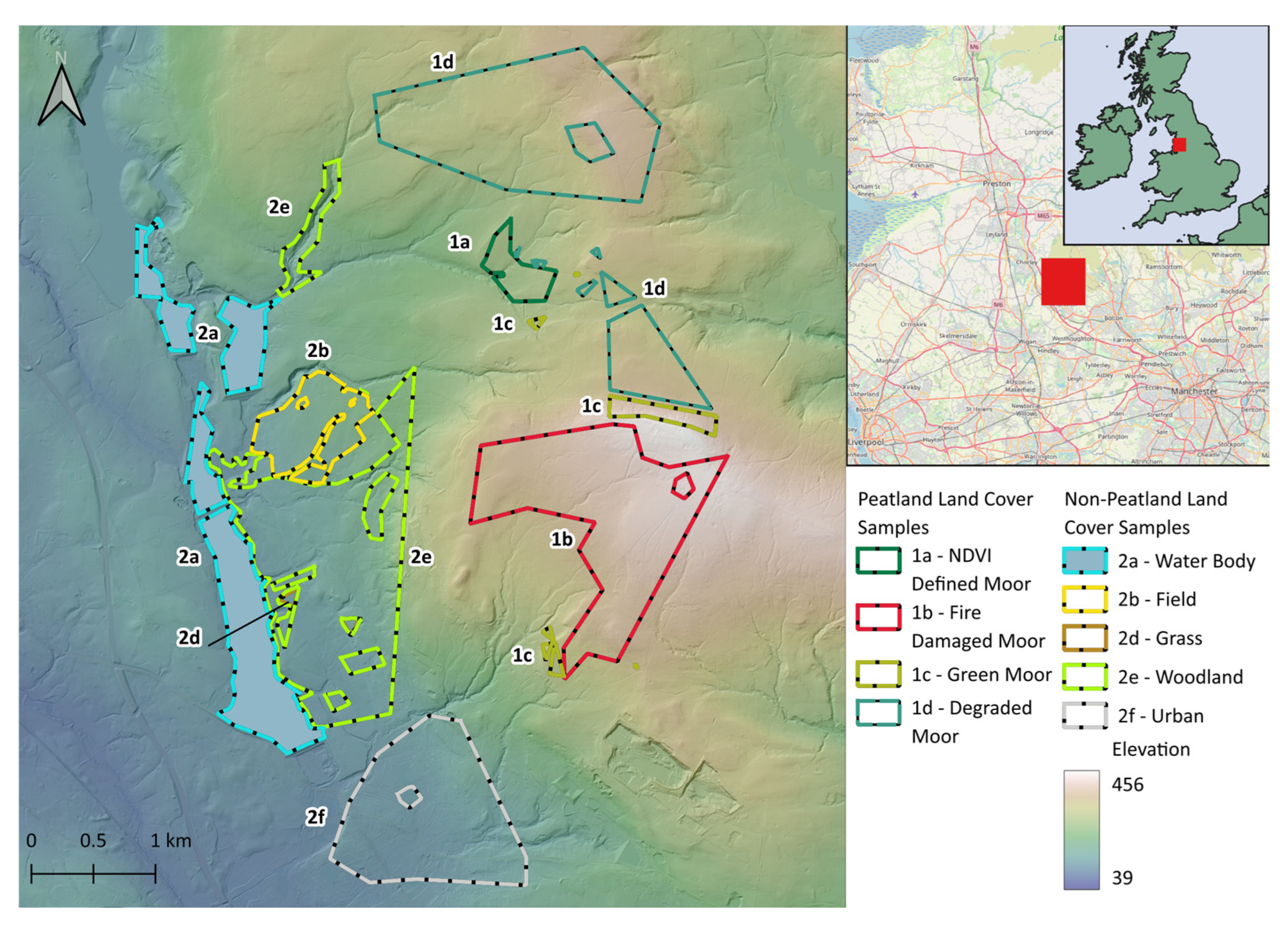
An area of interest (AOI) had already been located, where a moorland wildfire occurred at Winter Hill, on the Smithills Estate, near the Lancashire town of Bolton in the UK in July 2018. Elevation across the AOI ranges from 170 to 450 m above sea level. Figure 2 illustrates the topography of the area. Temperatures drop sporadically below 0 °C during winter in this region. A time series was identified for the study, commencing the winter before the wildfire in 2017/18 and up to 2023/24. European Centre for Medium-Range Weather Forecasts (ECMWF) reanalysed ERA5 data with a resolution of 0.1° (9 km) was obtained for temperature at 2 m above the Earth’s surface, to coincide with Sentinel-1 orbit pass dates applicable to the AOI. Daily temperature data at 6am was selected, as this aligned with the ascending satellite pass time. Sentinel-1A Interferometric Swath (IW) Level 1 Ground Range Detected (GRD) SAR imagery on the same orbit pass was then acquired for these dates, meeting the requirement for temperature at 6am to be below 0 °C. It is acknowledged that the low resolution of temperature data used may introduce error, but the AOI is one of the highest areas in the spatial extent of this dataset. The assumption that temperatures were below freezing on the applicable dates was therefore considered reasonably robust for using this data.

Table 1. Climatic conditions on Sentinel-1 image dates with chronology of the fire event and restoration works highlighted in bold.

Date	Temperature (°C)	Wind Speed (km/h)	Sentinel-2 Evidence of Surface Conditions	ERA5 Snow Cover (%)	ERA5 Snow Depth (m)	Precipitation (mm)
29/11/17	8.77	17	No snow coverage.	0	0.00	0
11/12/17	−3.50	10	Verified snow coverage on S-2 image.	12	0.01	0
July 2018	Winter Hill wildfire
18/12/18	9.04	30	No snow coverage.	0	0.00	0
23/01/19	−2.30	1	Verified snow coverage on S-2 image.	5	0.01	0
19/11/19	−1.75	9	Not verifiable with S-2 image due to dense cloud cover.	0	0.00	0
13/12/19	5.03	27	No snow coverage.	0	0.00	0
24/01/21	−2.50	8	Not verifiable with S-2 image due to dense cloud cover. Local media reported snow forecast on this date.	26	0.01	0
2021	Winter Hill peatland restoration works undertaken
07/01/22	−3.50	1	Not verifiable with S-2 image due to dense cloud cover. Local media reported snow forecast on this date.	9	0.01	0
09/12/22	−4.55	2	No corresponding S-2 image. No snow on image 1 day prior.	0	0.00	3
02/01/23	3.31	9	No snow coverage.	0	0.00	3
04/12/23	2.60	19	No snow coverage.	0	0.00	1

below sets out the scenarios represented by the Sentinel-1 images analysed and local weather conditions at the point of acquisition. For the dates where temperature was below 0 °C, snow coverage could not be verified in every image, even on the coldest recorded date of 9 December 2022. At these temperatures, it can be assumed that if there was no snow cover, there would have been heavy frost and ice deposits on all land surfaces, with shallow, smaller water features probably frozen over, possibly occurring more frequently in moorland areas.

A suite of samples was needed to represent the main land cover types in the AOI. These samples provided a test as to how Sentinel-1 displays different land cover in relation to peatland habitats, especially those most visually similar in optical imagery. Specific land cover samples were identified using a variety of different sources and were grouped into two broad categories:

1.

Peatland surfaces. This type of land cover should retain water very close to or on the surface throughout winter. Areas were subdivided as follows:

a.

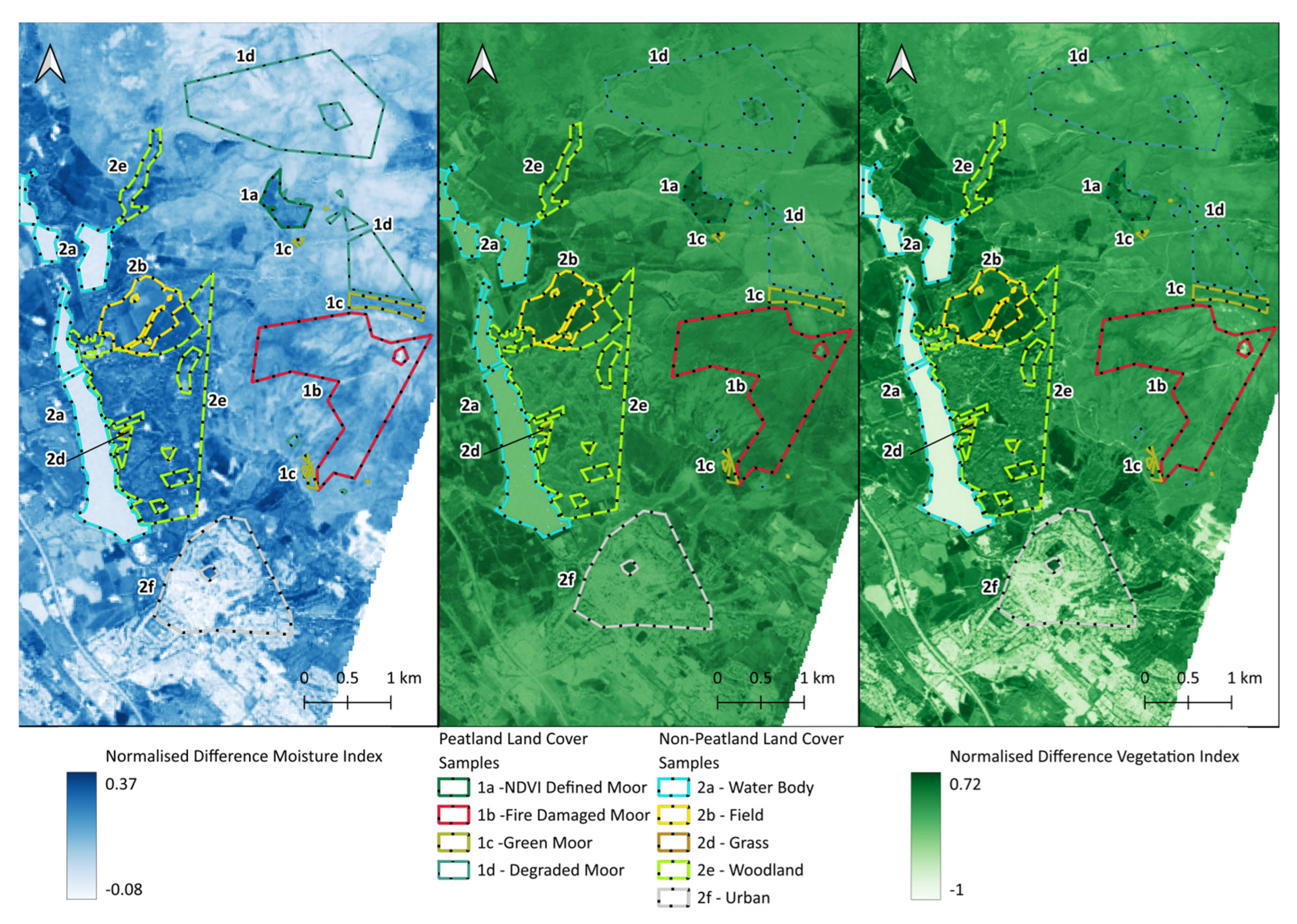
A site immediately north of Winter Hill that could be identified as moorland on satellite imagery, but which displayed more healthy vegetation according to Normalised Difference Vegetation Index (NDVI) values compared with other areas close to Winter Hill (see Figure 3). A Sentinel-2 optical image from December 2023 was used to calculate the NDVI. This land cover was named ‘NDVI Defined Moor’. It provided a benchmark as to how the restored moorland relates to moorland with relatively good vegetative health, as verified using NDVI.

b.

The area of moorland burnt in the 2018 wildfires. This sample was named ‘Fire-Damaged Moor’. The polygon was delineated by digitising the extent based on a Sentinel-1 image from the winter after the fire and comparing it with a map extract of the fire damage from the Woodland Trust, which owns the Smithills Estate. This area formed the basis of analysis to determine how relatively dry, degraded moorland, damaged by a large fire and then subject to restoration techniques, was characterised by θdB backscatter intensity.

c.

Visually healthy moorland, as identified from a field visit undertaken after heavy rain in October 2024. Samples were generated by digitising areas identified from georeferenced photographs, depicting relatively green vegetation that was not covered by any other sample extent. This land cover sample was named ‘Green Moor’. Figure 3 illustrates an NDVI image of the closest available cloud-free Sentinel-2 dataset to the site visit, which does not particularly distinguish this area from adjacent moorland. During winter though, Figure 3 also shows that these areas are characterised by higher Normalised Difference Moisture Index (NDMI) values than the surrounding moorland.

d.

Areas of brown grassland on the moor that were visually assessed as indicating dry peat soil in comparison to other parts of the AOI. This land cover was named ‘Degraded Moor’. Google Earth satellite images were used to digitise areas of brown grasses in moorland close to Winter Hill that had not been specifically affected by wildfires. Further samples were added during the October 2024 site visit at specific locations on the moorland around Winter Hill, where other areas of brown grass were also identified. A combination of satellite imagery and field visit photographic evidence produced a sample area amalgamated from 10 locations, mainly north of Winter Hill, but also including two southerly sites close to the Fire-Damaged Moor. Overall, this set of sample areas provided an opportunity to observe how visually assessed dry, degraded moorland can be characterised using Sentinel-1 backscatter in a frozen scenario, compared with better condition, i.e., wetter moorland. For example, due to the relatively dry state of the peat soil, does this sample more closely resemble an agricultural field?

e.

Sub-set samples within the sites of a, b and d above were also digitised after the October 2024 field visit, from which georeferenced photographs were taken in accessible locations to corroborate the use of these areas in representing respective moorland conditions. ‘Sub-Set’ has been appended to the areas these samples represent, for example, ‘Fire-Damaged Moor Sub-Set’.

f.

Another suite of sub-set samples was recorded within the sites of a, b, c and d on the field visit, specifically where streams and gullies were observed. ‘Stream’ has been appended to the areas in which these features are located, with a 50 m buffer creating a polygon around the point from which each photograph was taken. An example is ‘NDVI Defined Moor Stream’.

g.

Further sub-set samples were recorded where blanket bog was observed on the Degraded and Fire-Damaged Moor sites. Therefore, ‘Blanket Bog’ was appended to sample names to classify these areas.

h.

Two further samples were recorded for very small features, but which were considered to be of possible analytical value in future studies. The first was where planted saplings in moorland were observed on the site visit. Changes in backscatter over a longer period of time could provide some insight into how tree planting in peatland areas may affect this habitat. To maintain clarity in this paper, no results have been included for the planted saplings. The other site was a pit, probably manmade for low-scale peat production, that is identifiable from DEM data. This was considered relevant, as it is a common feature of peatland landscapes.

2.

Non-peatland surfaces, subdivided as follows:

a.

‘Water Bodies’, delineating permanent, relatively large lakes/reservoirs from Google Earth imagery. As these are large-area water surfaces, they did not freeze over on the dates analysed. However, backscatter in these locations may increase due to surface roughening by wind.

b.

‘Field’ delineating agricultural fields identified from Google Earth imagery. During the site visit it was observed that these fields are specifically used for sheep grazing. This sample provided the context of a natural surface, with similarly low-level vegetation to moorland, which Sentinel-1 C-band radar signals can easily penetrate. Grazing activity has kept vegetation low, with only small tussocks of more coarse grass observed sporadically covering the fields. This type of vegetative cover and the considerable surface water run-off witnessed on an adjacent road indicate that this surface is less permeable than moorland.

c.

Sub-sets of the ‘Field’ sample were photographed during the field visit, as agricultural fields vary in their use and hence their hydrological function within a landscape.

d.

‘Grass’, representing open informal recreational grass areas, i.e., not sports pitches. These areas were identified from photographs taken on the October 2024 field visit.

e.

‘Woodland’, delineating dense tree coverage, identified from Google Earth imagery. SAR C-band radar signals are less able to penetrate more dense vegetation. However, it is interesting to observe how these areas are represented by C-band backscatter in winter and during cold conditions.

f.

‘Urban’, delineating residential and industrial areas identified from Google Earth imagery. This sample provided evidence as to how SAR imagery represented impermeable artificial surfaces in freezing conditions, which will inevitably be warmer due to surface characteristics, plus building density and proximity.

g.

During the site visit substantial levels of surface water run-off were observed on some roads. Samples were therefore recorded for these surfaces, as their evident hydrological function in the drainage of landscapes should be considered.

Sentinel-1 data was acquired in verified frozen conditions and pre-processed in line with settings suitable to detect water surfaces [1]. Only images in VH polarisation were analysed, as this has been found to better delineate inundated surfaces [1].

Analysis was undertaken using QGIS software version 3.34 to create a raster layer for mean average backscatter intensity across the six images, from which a statistical profile could be developed for each land cover sample. Using boxplots to illustrate the interquartile (IQR) range of each land cover sample, revealed possible thresholds to delineate peatland from other land cover and ideally wetter from drier peatland. The smaller samples as described above, provided a more in-depth insight into how backscatter may represent areas that visually appear drier or conversely wetter, that more regularly hold surface water or contain features such as streams, trees or historic excavations.

These statistical profiles could then be used to symbolise different strata of backscatter values that may or may not correspond with the land cover samples and the sub-sets identified within them. This stratification method could be refined to identify wetter and drier peatland. The accuracy of this banded representation of peatland was assessed using visual observations from the field visit in October 2024. Comparing photographic records with a continuous surface map, symbolised according to sample boxplot ranges, would provide a subjective appraisal of accuracy in reflecting evident conditions. Other accuracy assessment methodologies using ground truth samples, such as temporal data of surface moisture levels, are not available, which generally supports this study’s motivation for using a remote sensing monitoring methodology.

In using the mean average of Sentinel-1 datasets in frozen conditions it was important to understand other climatic differences within the cohort. Snow cover could only be verified for four of the six dates used. Correlation between temperature and backscatter value was therefore tested overall and separately during known snow cover using the Pearson coefficient (r) and to gauge the fit of the data to a theoretical trendline, the overall coefficient of determination (r²).

Table 2. Land cover sample area and topography.

Land Cover Category	Land Cover Sample	Nr of Sites	Area (ha)	Slope °	Aspect	Topographic Wetness Index (% of Pixel Count)
						Least	Ave	Most
Peatland	1a—NDVI Defined Moor	1	17.27	6	West	12	79	9
	NDVI Defined Moor Sub-Set	6	5.78	7	West	10	85	5
	NDVI Defined Moor Stream	3	0.07	6	West	17	59	24
	1b—Fire-Damaged Moor	1	177.32	5	South-West	8	82	10
	Fire-Damaged Moor Sub-Set	3	0.92	13	South-West	23	77	0
	Fire-Damaged Moor Stream	1	0.07	8	South-West	43	29	28
	Fire-Damaged Moor Blanket Bog	1	0.18	2	South-East	0	100	0
	1c—Green Moor	7	14.17	19	North-East	25	73	2
	Green Moor Stream	3	0.08	9	West	33	34	33
	1d—Degraded Moor	10	228.94	6	South-East	9	80	11
	Degraded Moor Sub-Set	3	0.45	3	South-East	0	96	4
	Degraded Moor Stream	3	0.19	6	South-East	21	58	21
	Degraded Moor Blanket Bog	4	0.27	2	South	0	88	12
	Moor Pit	1	0.03	16	South	67	33	0
Non-Peatland	2a—Water Bodies	4	124.55	N/A	N/A	N/A	N/A	N/A
	2b—Field	1	49.28	5	West	4	84	12
	2c—Field Sub-Set	7	6.06	4	West	2	85	13
	2d—Grass	2	2.17	6	South-West	6	86	8
	2e—Woodland	5	223.38	8	South-West	16	72	12
	2f—Urban	1	142.77	4	South-West	9	77	14
	Road Surface	3	0.11	3	West	8	92	0

summarises the physical characteristics of the land cover samples, providing the area and number of sites used, as well as the average slope and aspect. The median average aspect was calculated to overcome the fact that there were multiple sites for some samples, therefore providing the predominant orientation. Topographic Wetness Index (TWI) is a GIS model that orders the hydrological topography of a landscape and was classified as follows:

• Most wet—All pixels with a TWI 1 standard deviation above the mean average;
• Average wet—All pixels with a TWI within 1 standard deviation of the mean average;
• Least wet—All pixels with a TWI 1 standard deviation below the mean average.

The formula to calculate the TWI is as follows:

$$ln{\displaystyle \frac{a}{\mathit{tan}b}}$$

where a is the local slope area draining into a cell and b is the cell area in radians.

All topographic data was derived using QGIS from a 2 m resolution Digital Terrain Model (DTM), acquired from the UK Department for Environment, Food and Rural Affairs (Defra) LIDAR catalogue and subsequently resampled to 10m resolution to match Sentinel-1 data.

TWI analysis was carried out to assess the relationship between backscatter intensity and the propensity for surface water to accumulate in an area. It must be noted however that the dates analysed were selected due to the low temperature at 6am, all of which were in generally seasonally dry periods. Where TWI has been used, albeit not in frozen conditions, it has been found to be effective in delineating peatland, as TWI values were higher in these areas [14]. In areas with higher TWI values, previous research indicates that backscatter should increase in peatland areas [8]. Testing these findings and comparing them with what happens in non-peatland areas could also help refine a delineation methodology. In terms of the other land cover samples, assessing the TWI for large water bodies is self-evident, for woodland, the ability of C-band radar signals to penetrate the canopy is low, even in winter and for urban areas the TWI is less relevant, as engineered drainage systems are present and by design are situated where surface water is most likely to accumulate.

Whilst TWI could provide an assessment of where water is likely to be retained in a land cover sample, segmenting these areas according to common hydrological relationships could also provide valuable insight. The DTM data was therefore used to define sub-catchment regions within each land cover sample. Sentinel-1 backscatter pixels within each sub-catchment would therefore be related in terms of their reliance on the same theoretical surface water draining point. Care was taken to ensure that these sub-catchments were refined enough that they took into account the surface drainage function of roads and paths. Zonal statistical analysis was therefore conducted to identify possible spatial patterns between Sentinel-1 backscatter and sub-catchment areas.

Slope is obviously integral to the construct of TWI and sub-catchments. However, it was considered that a simple classification exercise may also be a contributing factor in affecting Sentinel-1 backscatter response. Slope in degrees was calculated in QGIS from the 2 m resolution DTM and subsequently resampled to 10 m in line with the Sentinel-1 raster data. The resampled slope layer was then classified according to slope characteristics, as shown in

Table 3. Slope classes.

Slope Class	Slope Degrees (°)	Slope Category
1	0 < 1	Level
2	1 < 3	Very gentle slope
3	3 < 5	Gentle slope
4	5 < 10	Moderate slope
5	10 < 15	Moderate steep slope
6	15 < 35	Steep slope
7	>35	Very steep slope

.

Again, the relationship between these slope bands and backscatter response would be undertaken to identify any possible effects.

3. Results

3.1. Sentinel-1 Backscatter Relative to Peatland Condition

3-band raster compositions of seasonally similar Sentinel-1 backscatter images in VH polarisation of the Smithills AOI were compared in Figure 4 to illustrate the ability to delineate the wildfire burn extent.

The image on the left-hand side of Figure 4 includes three temporal bands of backscatter data immediately after the 2018 Winter Hill fire and on the right-hand side includes post-restoration data. The red rectangle highlights an area with similar changes in colour between the two images.

3.2. Comparison of Sentinel-1 Backscatter in Frozen and Non-Frozen Conditions

Figure 5 presents boxplots by main land cover class of the mean average Sentinel-1 backscatter for the six images captured in frozen conditions. It delineates the statistical zone between the 1st quartile of the Field sample, i.e., the 25th percentile of the data distribution (red dashed line) and the 3rd quartile of the Water Body sample, i.e., the 75th percentile (blue dashed line). Theoretically, the wetter conditions prevalent in a moorland habitat should determine that the IQR of these samples is situated within this zone.

Figure 6 presents boxplots for the same land cover classes of mean average Sentinel-1 backscatter for six images in non-frozen conditions.

In both Figure 5 and Figure 6, it is important to note that the Field IQR is most closely positioned to the peatland samples. Both the NDVI Defined Moor and the Fire-Damaged Moor IQRs are below the Field sample 1st quartile line in frozen conditions in Figure 5, providing a clear delineation threshold. However, for non-frozen conditions in Figure 6, there is an overlap.

The Green Moor IQR maintains a similar distance from the Field sample in both scenarios. The Degraded Moor also remains static in overlapping with the Field IQR, with the mean average similar to the Field 1st Quartile line in both scenarios.

Table 4. Key θdB backscatter statistics for other peatland land cover samples in frozen conditions.

Land Cover Sample	Number of Pixels	Mean	Median	1st Quartile	3rd Quartile	Range
NDVI Defined Moor Sub-Set	1175	−23.03	−22.98	−23.93	−22.21	10.21
NDVI Defined Moor Stream	112	−21.40	−21.17	−22.07	−20.52	5.45
Fire-Damaged Moor Sub-Set	225	−23.96	−24.00	−24.51	−23.48	6.00
Fire-Damaged Moor Stream	24	−23.28	−23.14	−24.00	−22.60	2.79
Fire-Damaged Moor Blanket Bog	45	−23.10	−22.76	−23.38	−22.57	4.01
Green Moor Stream	15	−20.16	−20.31	−21.09	−19.01	7.14
Degraded Moor Sub-Set	146	−21.46	−21.32	−21.91	−20.77	3.85
Degraded Moor Stream	45	−22.37	−22.97	−22.97	−21.77	2.62
Degraded Moor Blanket Bog	68	−22.84	−22.96	−23.23	−22.22	2.69
Moor Pit	6	−24.29	−24.22	−24.93	−23.42	2.12

summarises key backscatter statistics in frozen conditions for the sub-set peatland sites not represented as boxplots in Figure 5. The IQR of these sub-sets is generally well below the 1st quartile value for the field sample.

3.3. Delineation of Land Cover Classes by Sentinel-1 Backscatter in Frozen Conditions

The map in Figure 7 illustrates the use of land cover sample IQRs to delineate healthy peatland from similar land cover, such as grazed fields. A colour ramp has been defined using the following parameters to differentiate peatland applying Sentinel-1 backscatter average in frozen conditions, with the main land cover samples overlaid to demonstrate delineation:

• Blue—Sentinel-1 image minimum to Water Body quartile 3 (Q3) (−26.71 θdB);
• Green—Water Body Q3 (−26.71 θdB) to Degraded Moor quartile 1 (Q1) (−23.00 θdB);
• Orange—Degraded Moor Q1 (−23.00 θdB) to Field Q1 (−21.89 θdB);
• Red—Field Q1 (−21.89 θdB) to Grass Q3 (−18.68 θdB);
• Yellow—Grass Q3 (−18.68 θdB) to Woodland Q3 (−16.61 θdB);
• Black—Woodland Q3 value (−16.61 θdB) to Sentinel-1 image maximum.

The map in Figure 7 best differentiates healthier peatland areas (in terms of moisture content) by the turquoise shading, which is absent in the other land cover samples. However, the Field sample is generally shaded the same as more degraded (drier) areas of peatland locations.

3.4. Correlation Tests of Sentinel-1 Mean Average Backscatter and Land Surface Temperature in Frozen Conditions

To be able to confidently use these thresholds to delineate peatland and assess its relative condition, the statistical relationship between temperature and mean backscatter in VH polarisation needed to be examined.

Table 5. Correlation coefficient and coefficient of determination for mean average backscatter in VH polarisation and temperature in frozen conditions compared with non-frozen conditions for seasonally similar Sentinel-1 images from 2017 to 2022.

Land Cover Sample	Overall Correlation Coefficient (r)		Overall Coefficient of Determination (r2)
	Frozen Conditions	Non-Frozen Conditions	Frozen Conditions	Non-Frozen Conditions
Water Body	−0.87	−0.25	0.76	0.06
NDVI Defined Moor	0.50	−0.15	0.25	0.02
Fire-Damaged Moor	0.63	0.42	0.40	0.17
Green Moor	0.11	−0.64	0.01	0.41
Degraded Moor	0.40	−0.55	0.16	0.31
Field	−0.07	−0.06	0.01	0.00
Grass	0.22	0.37	0.05	0.14
Woodland	0.34	0.04	0.11	0.00
Urban	0.22	−0.45	0.05	0.20

tests this relationship using the r coefficient and to gauge the fit of data points to the trendline (r²). The correlation test has been compared for frozen and non-frozen conditions. Important observations to note are:

• Positive correlation, i.e., backscatter reduces as temperatures lower, is most evident in the Fire-Damaged Moor sample in frozen conditions (r = 0.63, r² = 0.40). In non-frozen conditions r = 0.42, but r² = 0.17.
• There is a negative correlation for the water body, i.e., backscatter increases as temperatures lower, which is strong in frozen conditions (r = −0.87), but weak in non-frozen conditions (r = −0.25, r² = 0.06).
• There is no correlation for the Green Moor sample (r = 0.11), or the Field sample (r = −0.07).

The difference between frozen and non-frozen conditions in the relationship between temperature and backscatter is illustrated using scatter graphs in Figure 8 and Figure 9. The Overall Coefficient of Determination (r²) for each class has also been included. Also included is a note to identify the Fire-Damaged Moor point for the Sentinel-1 backscatter image immediately after the wildfire. The trendlines generally indicate a positive correlation between temperature and backscatter in peatland habitats and no/little correlation in non-peatland areas.

To test the possible effects of slope on backscatter response, further analysis was conducted on land cover sample polygons adjusted to remove the two steepest classes 6 and 7 (see Table 3). Figure 10 below illustrates the trend in the relationship between temperature and backscatter, where the Green Moor now has a positive correlation (r = 0.36, r² = 0.13).

Correlation between temperature and backscatter was also tested for the other peatland classes as shown in

Table 6. Correlation coefficient and coefficient of determination for mean average backscatter in VH polarisation and temperature in frozen conditions by other peatland land cover classes for six seasonally similar Sentinel-1 images from 2017 to 2022.

Land Cover Sample	Overall Correlation Coefficient (r)	Overall Coefficient of Determination (r2)
NDVI Defined Moor Sub-Set	0.36	0.13
NDVI Defined Moor Stream	0.15	0.02
Fire-Damaged Moor Sub-Set	0.24	0.06
Fire-Damaged Moor Stream	0.71	0.51
Fire-Damaged Moor Blanket Bog	0.20	0.04
Green Moor Stream	0.12	0.01
Degraded Moor Sub-Set	0.54	0.29
Degraded Moor Stream	0.08	0.01
Degraded Moor Blanket Bog	0.44	0.19
Moor Pit	−0.18	0.03

below, together with the dispersal of data points in relation to a plotted trendline.

3.5. Accuracy Assessment of Sentinel-1 Mean Average Backscatter and Land Surface Temperature in Frozen Conditions

The small multiple set of maps in Figure 11 provides a larger scale representation of the map in Figure 7 in relation to photographic records from the field visit of October 2024. This formed the basis for a visual accuracy assessment as to how categorised Sentinel-1 backscatter depicted evident wet and dry peatland in a specific location.

Taking each of the maps in turn in Figure 11, starting from the top left and moving clockwise, key observations are as follows:

• NDVI Defined Moor
  • A noticeable area of coarse, green grasses within the sample area in the photograph can be depicted in a south-west direction as light turquoise shading following the magenta arrow on the map.
• Fire-Damaged Moor
  • Shorter, thick green grass areas are again distinguishable as turquoise areas in a broadly southerly direction from the arrow.
• Degraded Moor
  • The consistently brown grasses of obviously dry, degraded moorland are quite evident on the map by the orange and yellow shading in a broadly easterly direction.
• Degraded Moor (Foreground)/NDVI Moor (Background)
  • This photograph provides a fore and background perspective that can be verified on the map. In the foreground to the arrow moving broadly north-west, light brown grasses are represented in orange and very light brown shades, whereas, the background green grasses are shown in turquoise further north-east on the map.
• Degraded Moor (Foreground)/Green Moor (Background)
  • In the photograph there is noticeable brown moorland, behind which is greener moorland as the land rises in elevation. The map illustrates swathes of orange shading stretching south-east from the arrow. There are though small patches of turquoise scattered throughout this area, but the green moor is distinguishable on the southern border of the map.
• Grass
  • The grass sample in the photograph does not seem to have a particular use other than casual recreation, such as dog walking and as the vegetation is short, possibly regularly maintained. On the map, the sample is a slightly lighter shade of orange. Boundary woodland that can be seen in the photograph is depicted well in yellow shades.
• Field
  • This field is used for sheep grazing and appears to have had no land use changes in historic satellite images. It is generally represented in orange shades on the map.
• Degraded Moor Blanket Bog
  • This comparison indicates how specific habitat changes where surface water is more prevalent have been detected by Sentinel-1 backscatter. The photograph shows the boggy conditions that are represented in blue and vivid turquoise in the map. As previously mentioned, it is interesting to note that the blanket bog sub-set samples, located in otherwise dry peatland areas, have quite different backscatter profiles, as Table 4 demonstrates. The 3rd quartile value for these blanket bogs is below the mean average for the Degraded Moor sample overall.

3.6. Correlation Tests of Sentinel-1 Mean Average Backscatter and Land Surface Temperature in Snow Cover

Table 7. Correlation coefficient and coefficient of determination for mean average backscatter in VH polarisation and temperature during snow cover for four seasonally similar Sentinel-1 images from 2017 to 2022.

Land Cover Sample	Correlation Coefficient (r)	Coefficient of Determination (r2)
Water Body	−0.81	0.66
NDVI Defined Moor	−0.92	0.85
Fire-Damaged Moor	0.76	0.58
Green Moor	0.11	0.01
Degraded Moor	0.59	0.35
Field	0.28	0.08
Grass	−0.93	0.86
Woodland	−0.62	0.39
Urban	−0.71	0.50

below tests the statistical relationship between mean backscatter in VH polarisation against local temperature at 2 m above the Earth’s surface, at 6am on the date of image capture on four dates when there was verified snow cover. Key observations to note are:

• Positive correlation, i.e., backscatter reduces as temperatures lower, is still most evident in the Fire-Damaged Moor sample in frozen conditions (r = 0.76). The Degraded Moor also displays a fairly strong correlation (r = 0.59).
• This time, a peatland sample, the NDVI Defined Moor, also displays a strongly negative correlation (r = −0.92), i.e., backscatter increases as temperatures lower. This is also the case for all but the Field sample of the non-peatland land cover.
• The Green Moor sample again displays no relationship (r = 0.11) and the Field sample correlation is very weak.

The scatter graphs in Figure 12 and Figure 13 also focus on when there was verified snow cover to identify any differences with overall frozen conditions. Whilst only 4 datasets have been analysed there is an observable difference in the relationship between peatland and non-peatland surfaces. Apart from the NDVIDefined Moor, peatland surfaces in Figure 13 display varying positive correlation between backscatter and temperature. In Figure 12 all non-peatland surfaces (apart from the Field sample) display a negative correlation.

In

Table 8. Correlation coefficient and coefficient of determination for mean average backscatter in VH polarisation and temperature in snow cover by other peatland land cover classes for four seasonally similar Sentinel-1 images from 2017 to 2022.

Land Cover Sample	Overall Correlation Coefficient (r)	Overall Coefficient of Determination (r2)
NDVI Defined Moor Sub-Set	−0.95	0.91
NDVI Defined Moor Stream	−0.50	0.25
Fire-Damaged Moor Sub-Set	−0.87	0.76
Fire-Damaged Moor Stream	0.74	0.55
Fire-Damaged Moor Blanket Bog	0.12	0.01
Green Moor Stream	−0.37	0.14
Degraded Moor Sub-Set	0.00	0.00
Degraded Moor Stream	−0.73	0.54
Degraded Moor Blanket Bog	0.97	0.94
Moor Pit	−0.49	0.24

below the relationship between backscatter and temperature has been tested in snow cover for the other peatland samples.

3.7. Sentinel-1 Mean Average Backscatter by Hydrological Classification

In testing areas within each sample by their propensity to accumulate water using TWI values, the wettest areas were expected to have the highest backscatter [14]. The bar chart in Figure 14 shows the mean average Sentinel-1 backscatter for each land cover sample across the six images dates in areas considered to be most wet, averagely wet and least wet as defined by the TWI value for each 10 m × 10 m pixel within the sample polygons. For all of the peatland samples, the wettest areas had the highest backscatter profile, decreasing generally for the average and least wet classes. However, non-peatland areas displayed much less pronounced patterns of backscatter response compared with TWI class.

Figure 15 below represents the other peatland land cover samples by TWI category. These samples were much smaller in area, hence may not include all TWI categories. Generally, all of the sub-sets were similar to the main peatland samples in displaying higher backscatter in the wettest areas.

Each main land cover sample, apart from the Water Body, has been segmented by sub-catchment area in Figure 16 to create another hydrological perspective of Sentinel-1 backscatter across the six images capturing frozen conditions. This map uses blue shading to depict sub-catchments where the mean average backscatter is below −23.00 θdB, ordinarily depicting healthy peatland and orange shading where the mean average is between −23.00 and −21.89 θdB, which should delineate degraded peatland.

To understand the effect of segmenting backscatter by sub-catchment region, the standard deviation has been compared with that of the overall land cover sample area below in Figure 17. Each sub-catchment in the land cover sample areas was categorised as being higher or lower than the overall sample standard deviation.

3.8. Sentinel-1 Mean Average Backscatter by Topographic Classification

In Figure 18 the mean average backscatter by slope classification has been plotted across all main land cover samples to identify possible differences between each surface in relation to terrain. The Grass sample is not represented, as segmentation by slope resulted in very small sample areas that were not comparable with the relatively large segments of other classes. Analysis found that backscatter generally decreased as slope increased. This was also the case for all other land cover, except woodland (the woodland canopy, which is what is detected by Sentinel-1 backscatter, is obviously less affected by slope).

Figure 19 below shows segmented land cover samples by landform feature, with the mean average backscatter in each, depicted by the bar lengths in the chart. Landform features have been arranged in order of slope characteristics from low to high. That is, starting from the left are surface depressions, followed by flatter ground forms and on the right-hand side the highest features in a landscape, culminating in a peak. The most common landform feature in each land cover sample has also been plotted with the round markers.

4. Discussion

4.1. Fire Damage Delineation

When displayed in a 3-band raster image, Sentinel-1 backscatter in VH polarisation clearly delineates the effects of the 2018 Winter Hill wildfire. The visual differences in the 3-band raster images in Figure 4 quite accurately display the burn extent outlined in black and white, therefore effectively distinguishing fire-damaged peatland by the significant increase in backscatter detectable in the image recorded the winter immediately after the wildfire. However, there are areas of the map where changes can be detected that are visually similar to the moorland burn extent. An example is outlined with a red rectangle in the north-western region of the map. Another less noticeable example is the Field sample area, symbolised with the yellow dashed line. It is very unlikely that these areas were anymore affected by the wildfire than other parts of the AOI. Whilst Sentinel-1 backscatter in VH polarisation potentially provides a delineation approach to distinguish fire-damaged peatland, more detailed analysis is required to understand if this is also applicable for the overall peatland condition. It is recommended that future research focuses on whether observed backscatter changes also occur for other similar surfaces, such as agricultural land used for grazing.

4.2. Statistical Threshold Delineation of Peatland Habitat

As peatland has a greater ability to retain surface water than other natural land surfaces, scenarios that better display these abilities are perhaps the most favourable conditions by which to distinguish peatland from similar land cover and potentially delineate wet, healthy from dry, degraded habitat.

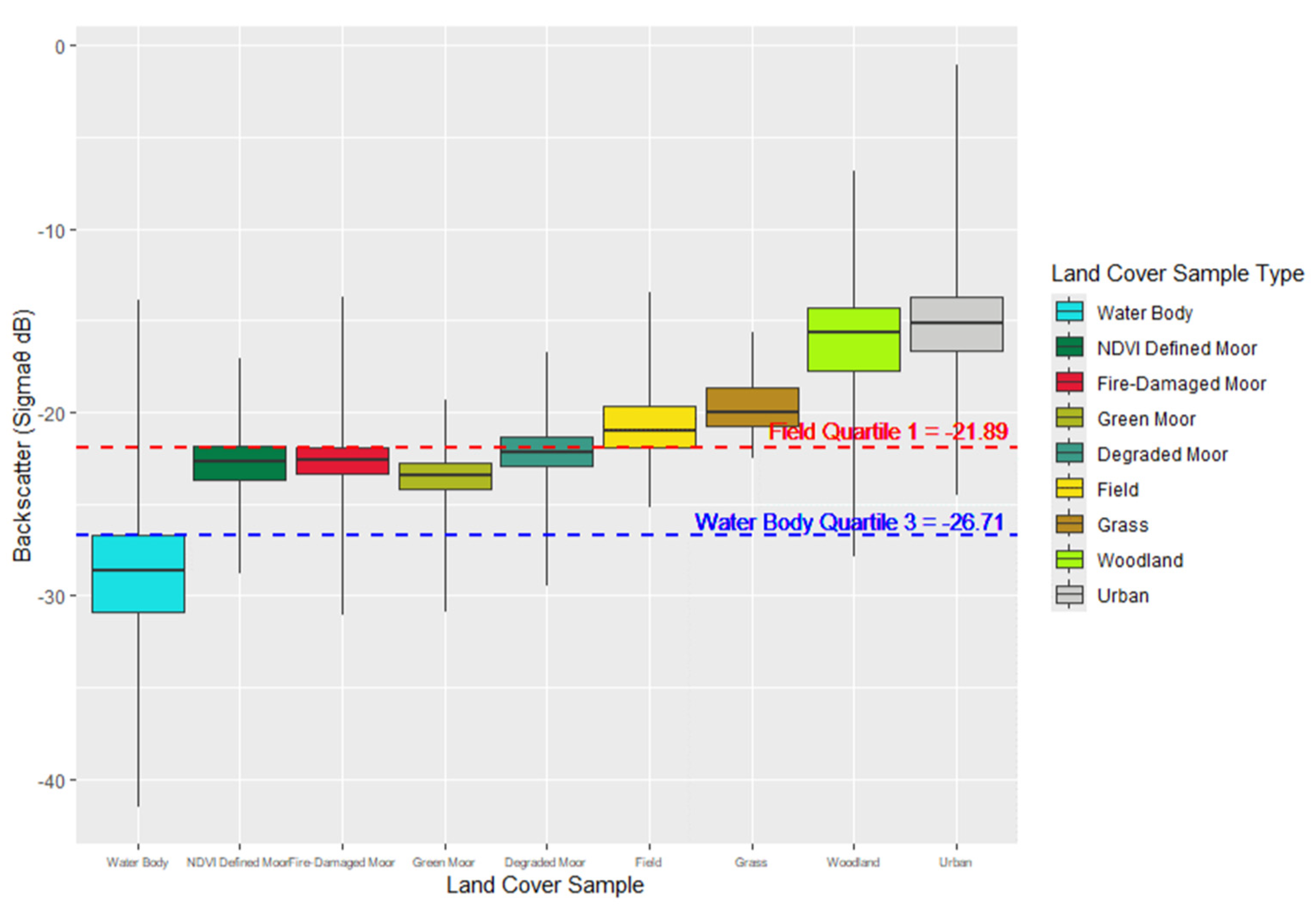
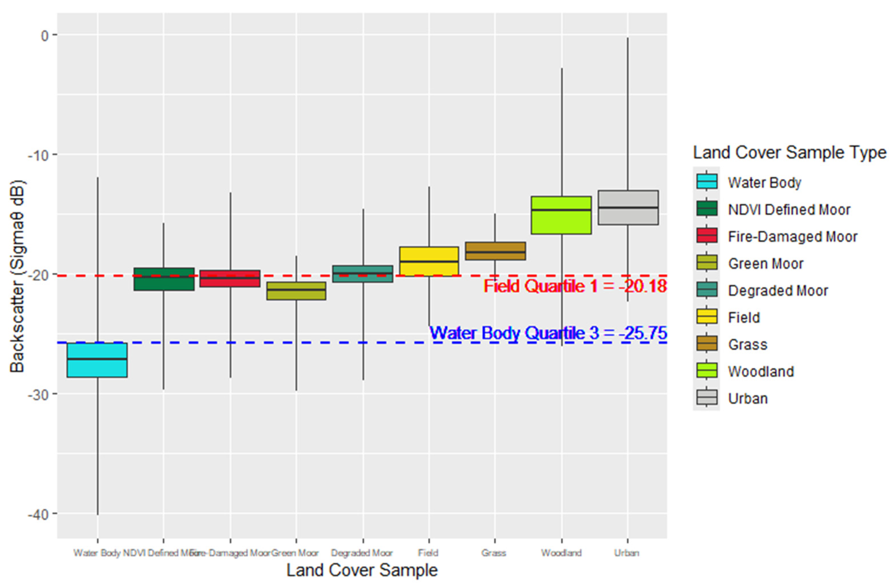
Analysis of Sentinel-1 backscatter values across six seasonally similar dates between 2017 and 2022 has shown that there is a distinct difference between peatland sample sites compared with non-peatland sites, when local temperature 2 m above the ground is below 0 °C. When comparing Figure 5 and Figure 6, it is noticeable that all of the land cover backscatter mean averages, except the Woodland and Urban categories decreased in frozen conditions, verifying previous findings [18]. More importantly, Table 5 indicates some positive correlation between backscatter and temperature using the r coefficient for all peatland surfaces except the Green Moor. This is in stark contrast to non-peatland surfaces where there is no real relationship, i.e., backscatter has decreased when temperatures were below 0 °C, but in no particular pattern. Indeed, the Field sample results were similar to other research in frozen conditions [20], but in this study, it has been shown that only a reduction can be predicted, not what happens if, for example, the temperature is −1.2 or −4.5 °C.

In this AOI, land cover dedicated to agricultural use is the most similar to peatland. Using the IQR for the mean average across the six dates analysed for each 10 m × 10 m pixel within a land cover sample in frozen conditions, Figure 5 demonstrates minimal overlap of the Field land cover sample with peatland. Peatland surfaces are generally positioned between the Field and Water Body samples. A logical notion when considering how functional peatland is construed as ‘wetland’, i.e., acting as a sponge-like surface that in terms of water retention sits between natural low-level vegetation such as agricultural fields and a water body. When temperatures are above freezing, this distinction of peatland from the Field IQR is less clear, as can be seen in Figure 6.

In analysing the frozen scenario of boxplots in Figure 5 in more detail and also in comparison with the non-frozen dataset in Figure 6, there are some interesting observations to note:

• In frozen conditions, the NDVI Defined Moor IQR does not overlap at all with the Field sample, which is unsurprising when considering that Sentinel-2 data distinguished this area by its apparent vegetative health (see Figure 3). Above 0 °C the situation was very different, as the IQR position shifted upwards to overlap with the Field IQR, with the mean average (marked with a horizontal line) almost equal to the 1st quartile value of the Field sample. A point to note is that the NDVI Moor has a slightly larger IQR than other moorland sites in both scenarios, although it is still noticeably smaller than the Field and Grass samples. It can therefore be assumed that where winter NDVI values are high in peatland areas, there is a noticeable differentiation from agricultural grazing land in terms of backscatter. Sub-sets of the NDVI Moor sample generally fall within the main IQR range as shown in Table 4. However interestingly the sub-set adjacent to a stream does have relatively higher backscatter. This is a very small sample though.
• In both scenarios, the Fire-Damaged Moor sample sits within the NDVI Defined Moor IQR, generally aligning with its 3rd quartile and overall is higher than the Green Moor IQR. It is also below the Field 1st quartile line in frozen conditions. Again though, above 0 °C the IQR position shifted upwards into the Field IQR zone. Whilst the Fire-Damaged Moor IQR is closer to that of the Field in conditions above 0 °C, its position and size relative to other peatland samples is surprising considering that this site was historically dry and degraded and suffered extensive fire damage (the effect of which is illustrated in Figure 9, where the post-fire average backscatter point is markedly higher than all other peatland markers), before undergoing restoration work to rewet the peatland. Again, there is a difference for peatland where restoration activity has taken place. Table 4 shows all the Fire-Damaged Moor sub-sets to be fairly similar to the main sample IQR.
• The Green Moor sample had the lowest IQR of all the peatland surfaces in both scenarios. Whilst not particularly well represented by NDVI images (see Figure 3), these areas show up well using NDMI, although the Field sample also has a high NDMI. A point to note is that this main peatland sample has by far the steepest slopes (see Table 2, 19° compared with less than 10° for all other main classes). This is reflected in the Green Moor having the lowest proportion of TWI pixels classified as the most topographically wet (2% compared with an average of 10% for the other main peatland classes, also in Table 2). Conversely, this sample is the cohort with the lowest backscatter values, despite having the least favourable topography for water retention. It is also the most northerly facing of the peatland samples. This supports the assertion that wetter peatland (as evidenced by an abundance of green vegetation) displays a noticeable difference in backscatter to similar land cover in frozen conditions.
• Predictably, the Degraded Moor was the only peatland IQR to overlap with that of the Field sample in both scenarios. The mean average was outside the Field IQR extent in frozen conditions, but fell within it when temperatures were above 0 °C. Sub-sets within the Degraded Moor sample where there was evidence of wetter conditions (bog and stream samples), displayed relatively low backscatter profiles. Further evidence that wetter conditions in peatland can be identified by backscatter in frozen conditions. Overall, these findings support the possibility of differentiating between wet and dry condition peatland according to backscatter in frozen conditions.
• Of the non-peatland samples, the Field land cover IQR was most closely situated to the peatland boxplots in both scenarios. This offers the potential for a suitable minimum threshold from which to delineate peatland habitats using Sentinel-1 backscatter in frozen conditions. There is not such a clear separation when temperatures were above 0 °C.
• The Grass sample IQR was positioned at the upper extent of the Field sample in both scenarios. Interestingly, there is a greater spread of backscatter distribution in frozen conditions. These observations indicate that areas with shorter, more maintained vegetation may have a more differentiated average backscatter profile to peatland habitats in frozen conditions. In comparison, this sample had a less favourable TWI to that of the Field sample (see Table 2, 8% most wet proportion compared with 12%), which supports why the IQR was higher positioned.

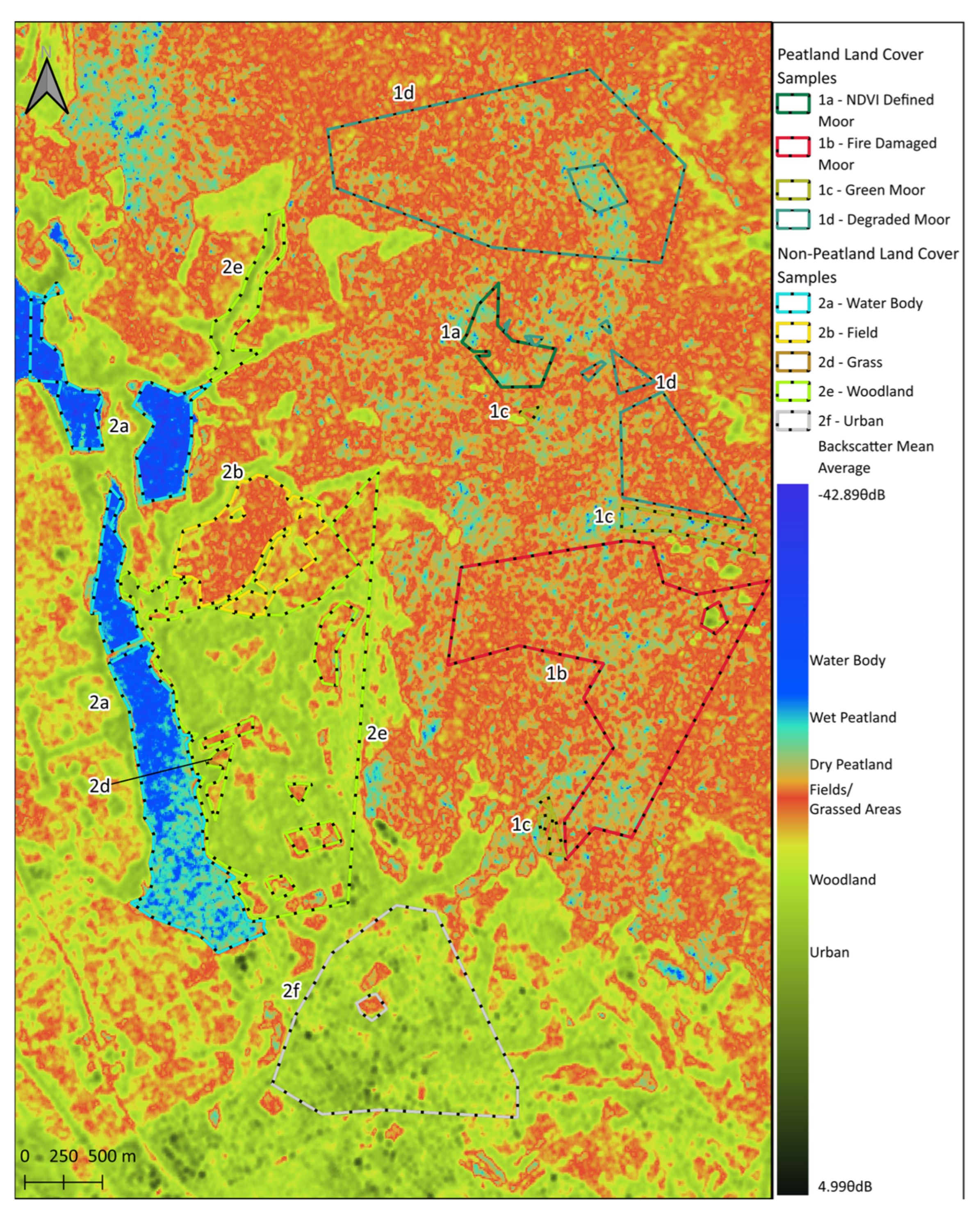
The boxplots in frozen conditions in Figure 5 clearly illustrate how the IQR range of peatland resides between the Water Body and Field/Grass land cover samples and may even offer the potential to delineate dry, degraded from wet, healthy peatland. This clarity does not exist in conditions above 0 °C (Figure 6), where there is some overlap in all the peatland samples, except the Green Moor. 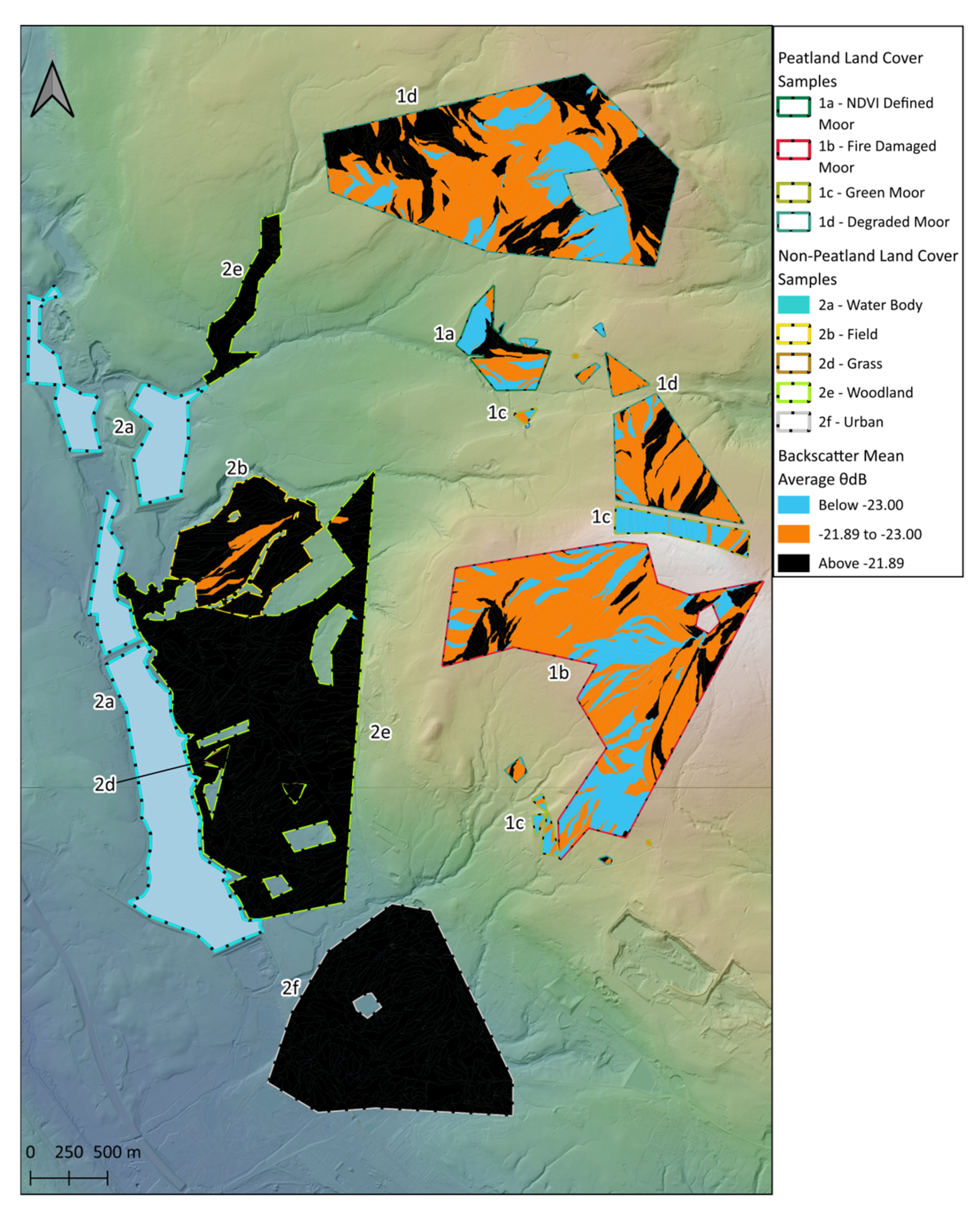In practice, however, using the map in Figure 7 to spatially represent theoretical bands identified from the boxplots in frozen conditions, such as between Water Body Q3 and Field Q1, is less definitive in delineating peatland. As expected, there is a clear differentiation of peatland from woodland and urban areas, but this is easily achievable with any optical imagery. The colours within the Field area (annotated as 2b), represented by the yellow dash/black dot line in Figure 7 and, for example; large parts of the Fire-Damaged Moor (red dash/black dot, annotated as 1b) are very similar, making it difficult to differentiate between these land cover classes. This is also the case for the Degraded Moor sample, although the overlap in boxplots in Figure 5, makes this less surprising.

An interesting aspect of the map in Figure 7 is the turquoise regions, for example: scattered through the Fire-Damaged Moor sample; the predominance in the Green Moor area (1c); the peripheral areas of the NDVI-Defined Moor (1a) and the north–south orientated band within the large Degraded Moor extent (1d). This, along with the lower backscatter in sub-sets of the Degraded Moor sample, where wetter conditions are evident may well indicate the probable variation in peatland condition across all the samples.

4.3. Sentinel-1 Backscatter/Temperature Correlation

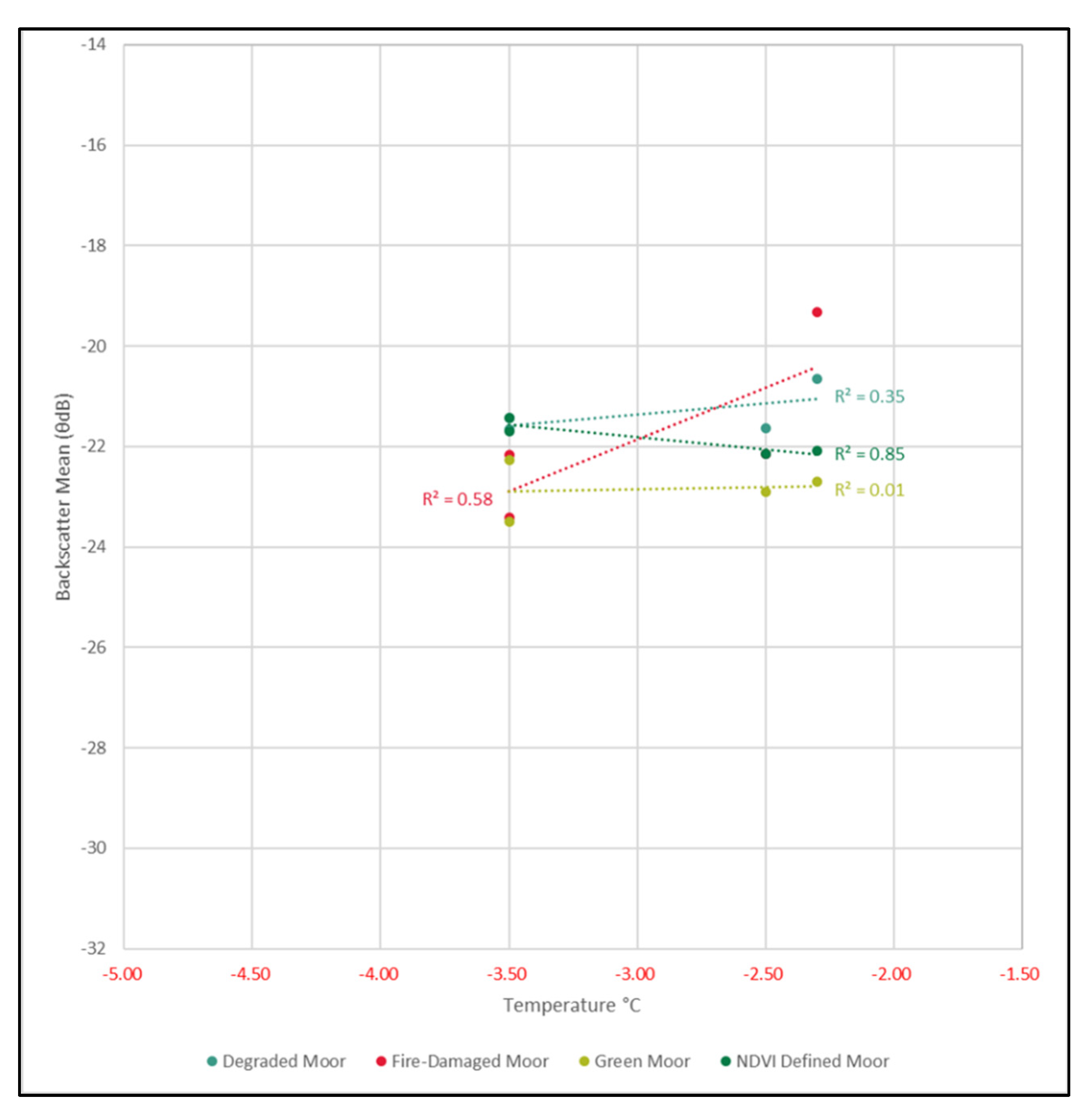
The statistical relationship between temperature below 0 °C and backscatter for the peatland samples is mixed, but as set out in Table 5 is very different in comparison to when temperatures were above 0 °C. As determined by the correlation coefficient r, there was a positive relationship for the NDVI Defined Moor, i.e., backscatter increased with temperature, but there was no correlation above 0 °C. For the Fire-Damaged Moor, there was a positive correlation in frozen conditions, which was less defined above 0 °C. As may be expected for the Degraded Moor sample, there was a slightly less positive correlation, but this was negative above 0 °C. For the Green Moor, there was almost no relationship in frozen conditions, but a relatively strong negative relationship above 0 °C. It should be noted that other peatland samples displayed even greater variance in relationship between backscatter and temperature when conditions were above 0 °C. For example; the NDVI Defined Moor changed from a positive to no real relationship, the Degraded Moor completely changed from a weakly positive relationship to a relatively strong negative one.

The different topography and aspect of the Green Moor may be a factor in why this sample produced relatively low backscatter irrespective of temperature when below 0 °C. Figure 10 to some degree explains how the steepness of this sample affects backscatter, as when the steepest slopes were removed a relatively weak positive correlation was recorded (r = 0.36, r² = 0.13).

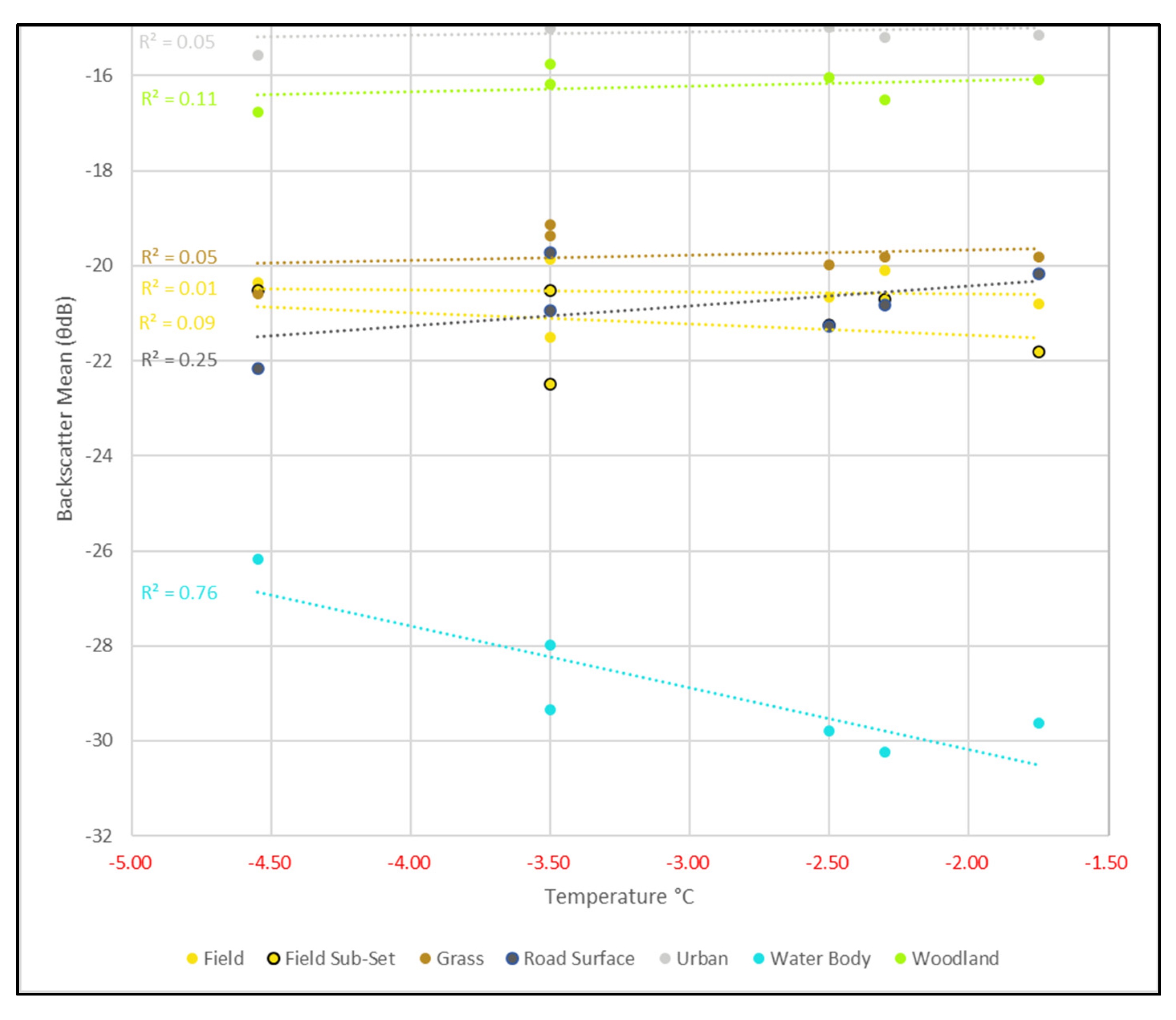
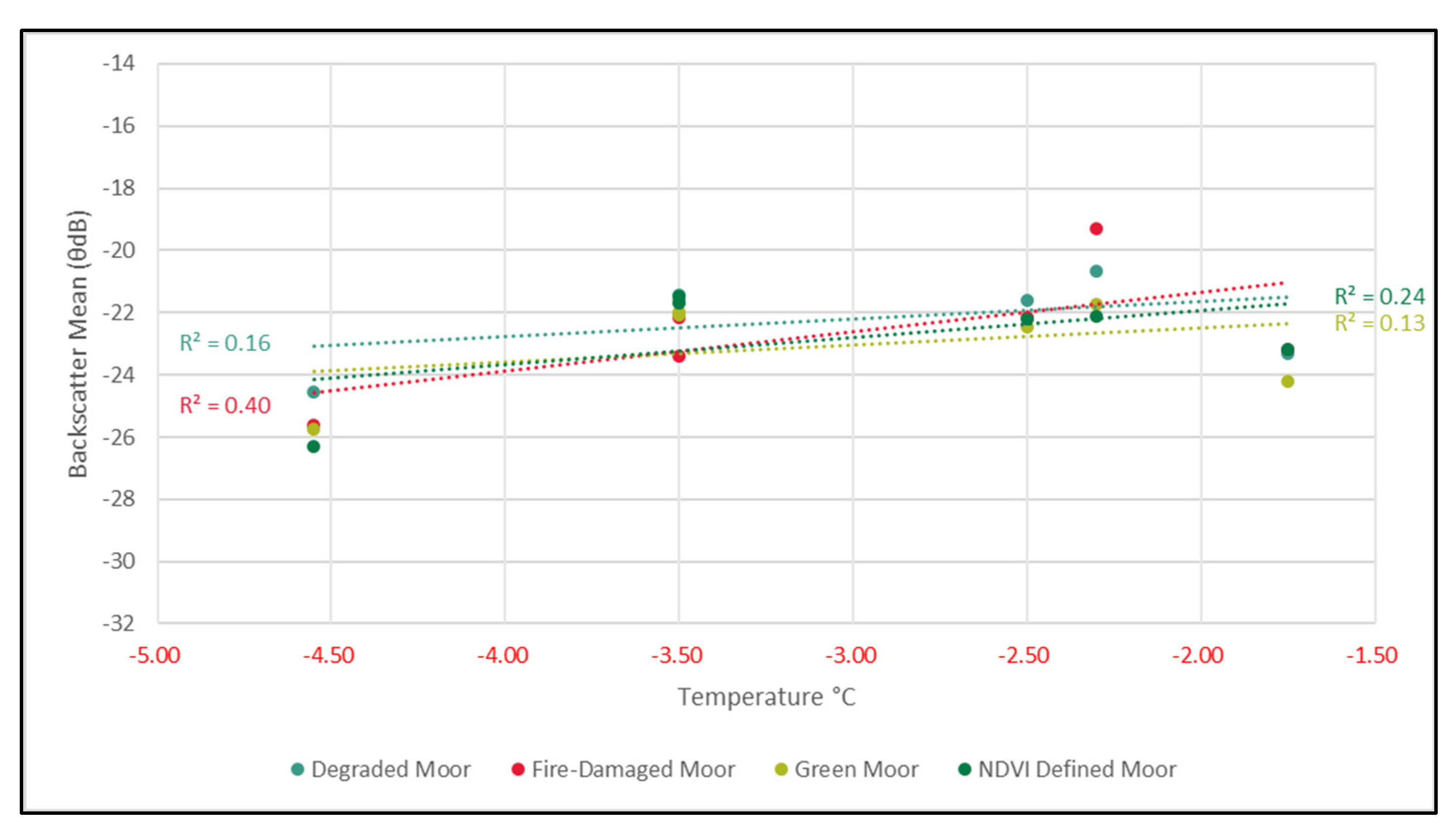
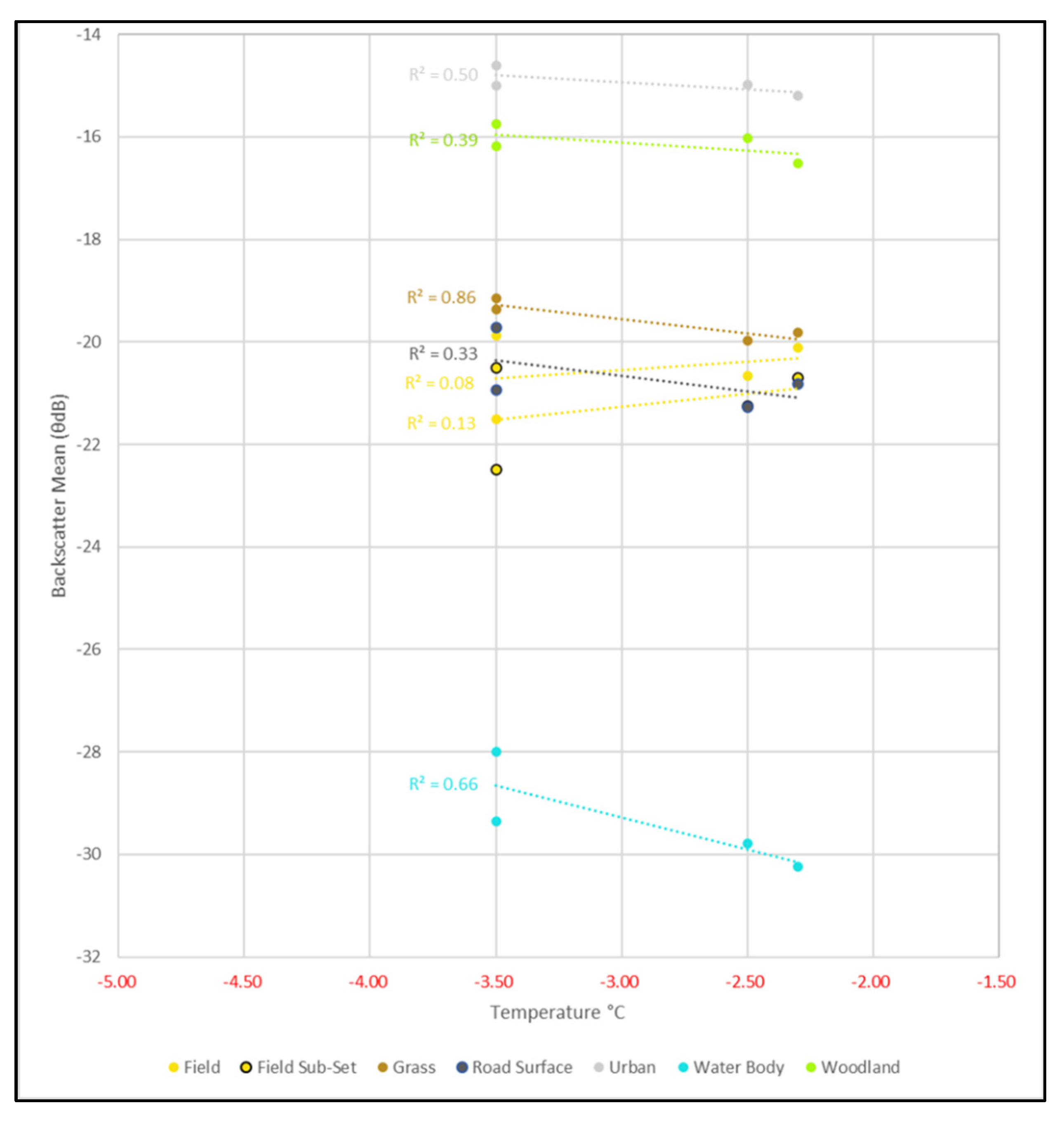
Looking in more detail at possible correlation of backscatter and temperature in frozen conditions, aside from the Green Moor, peatland samples are distinguishable from non-peatland areas when comparing Figure 9 with Figure 8, but their general trendline fit (r²) is poor.

It is worth noting that the two small non-peatland samples included in Figure 8, the Field Sub-Set and Road Surface, were derived from site visit observations and generally fit with the overall summary of non-peatland surfaces in frozen conditions. This was also the case in Table 6, where smaller peatland samples also derived from the site visit, generally displayed a weak positive correlation between backscatter and temperature, reflecting the main peatland sample sites.

Interestingly, the only sample that had a negative relationship between backscatter and temperature in frozen conditions was the Water Body. Wind speed records in Table 1 do not appear strong enough to indicate possible roughening of the surface due to waves on these dates. Although, this should not be ruled out, as it is likely that conditions may differ locally across the water features sampled.

When the data in frozen conditions was separated to look at those dates where there was verified snow cover in Figure 12 and Figure 13, the relationship between backscatter and temperature abruptly changed in the NDVI Defined Moor, Field, Grass, Woodland and Urban samples. Table 7 demonstrates that there was a strong negative correlation, i.e., backscatter increased when temperature decreased for all non-peatland surfaces, except the Field sample. In assessing backscatter where there was snow cover, it is not known how consistent or thick the snow layer was in this area, as this would have varied according to local conditions. However, what is plain is that in snow cover, the backscatter profile for these surfaces reacted differently according to temperature than overall for frozen conditions. The trendline fit (r² value) for all of these surfaces was also good. It must be noted though, that this was also the case for the NDVI Defined Moor sample. Theoretically, wet snow, which is typical in this locality would produce lower backscatter, however melting snow would increase backscatter [17]. All of the land cover where the correlation changed were predominantly westerly or south-westerly facing. It is therefore probable that localised snow conditions affected backscatter in these areas.

The positive relationship and trendline fit between backscatter and temperature actually improved for the Fire-Damaged Moor and Degraded Moor samples. These have predominantly south-west and south-east aspects, respectively. The Green Moor correlation coefficient was unchanged, displaying no real relationship. This sample faces north-east.

There were also fundamental changes for the smaller peatland samples in snow cover, as Table 8 demonstrates. The correlation generally switched, with a relatively good trendline fit in most cases. For the NDVI Defined Moor Sub-Set this was not surprising, as this also formed part of the main NDVI Defined sample and was also the case for the NDVI Defined Moor Stream, although the trendline fit in this instance was poor. It was not expected though that the Fire-Damaged Moor Sub-Set would be different to the main Fire-Damaged Moor sample, as this displayed a strong negative relationship between backscatter and temperature (backscatter decreasing when temperature increased). There was though a difference in the TWI classification for these two samples, as in Table 2 the Fire-Damaged Moor Sub-Set had no coverage classed as ‘most wet’, whereas the main sample ‘most wet’ coverage was 10%. This was also the case for the Degraded Moor Stream sample, which had the highest proportion of ‘most wet’ pixels. It is worth noting that both these sites are small in area.

What can be interpreted from these observations, is that there is a difference between how peatland surfaces react in terms of radar backscatter compared to those surfaces most obviously similar, i.e., shallow water bodies and fields. Backscatter in the Field sample did not display any correlation in frozen conditions, whereas peatland surfaces generally did (the Green Moor being the exception, which may be related to topographic differences). What is not explainable is that this relationship fundamentally changed for the NDVI Defined Moor when there was snow cover, in line with non-peatland surfaces (except the Field sample). These exceptions aside, it is possible that a greater prevalence of water retained on peatland surfaces, provides the potential for Sentinel-1 backscatter to delineate these habitats from others.

4.4. Accuracy Assessment of Statistical Threshold Delineation

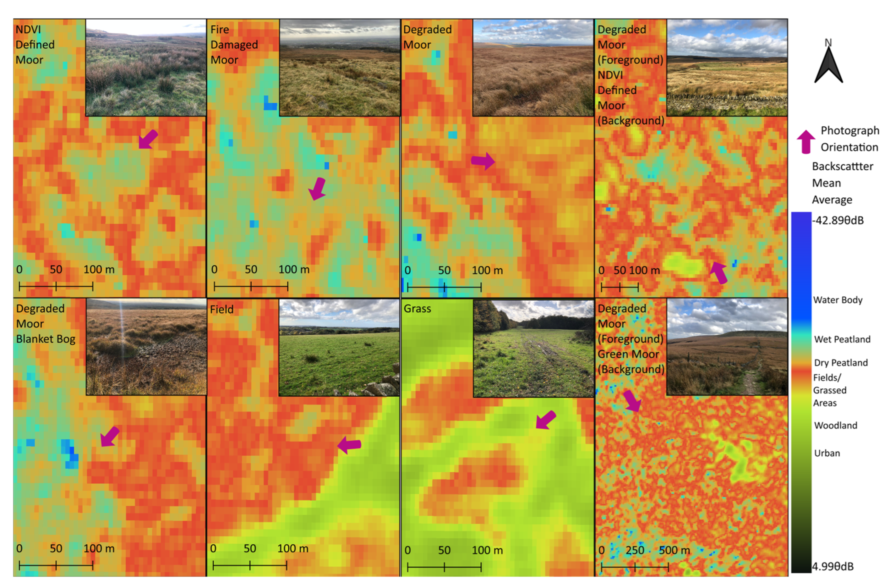
With no ground truth data available to assess peatland coverage and condition the small multiple map in Figure 11 is an interesting tool for comparison of field visit photographic records against the map of apparently wet, healthy and dry, degraded peatland in Figure 7, where classification used statistical thresholds. What has been assumed in this comparison though is that the areas photographed in October 2024 were in the same condition as when the datasets of Sentinel-1 images were captured between 2017 and 2022. With this assumption in mind, the comparison in Figure 11 does strongly support the view that Sentinel-1 backscatter provided a reasonable representation as to the condition of peatland.

Representing wet and drier peatland with these colour gradients, based on key statistical extents of land cover samples, is consistent with the photographic evidence. It is accepted that visual assessment is subjective, but records were carefully selected to represent only the most obvious signs of wet and dry conditions.

4.5. Delineation by Peatland Condition

Quite why wetter, better-condition peatland should display lower backscatter values needs further examination. Theoretically, inundated surfaces should emit higher backscatter, due to the effect the water surface below vegetation has in increasing the return of radar signals to a SAR sensor. This should therefore apply to the peatland samples witnessed in the site visit, as the vegetation cover was generally coarse grasses. Perhaps the propensity for peatland soils to hold moisture in frozen conditions translated into lower backscatter signals and was generally most pronounced where water retention was more probable. This premise is supported by the fact that of the six blanket bog and stream sub-set samples in Table 4, the mean average backscatter was lower than the main sample on four occasions. Whilst not significant, this does support the assertion that wetter peatland surfaces are even more likely to generate less backscatter. In mentioning backscatter response to vegetation cover, it is worth noting that the Woodland sample results categorically proved that tree canopies generate a relatively high backscatter response (see Figure 5 and Figure 6).

In seeking to distinguish wetter from drier, degraded peatland and other closely resemblant land cover classes, spatial representation of Sentinel-1 data alone provides questionable delineation results. The map in Figure 7 may well indicate a heterogeneous pattern of peatland conditions in the AOI, but it may also present other underlying factors that may lead to misinterpretation of Sentinel-1 backscatter in accurately reflecting wet, healthier and dry, degraded habitat. Further analysis was therefore required to better understand other underlying aspects. Hydrological characteristics and terrain were therefore considered as to whether they affected Sentinel-1 backscatter patterns.

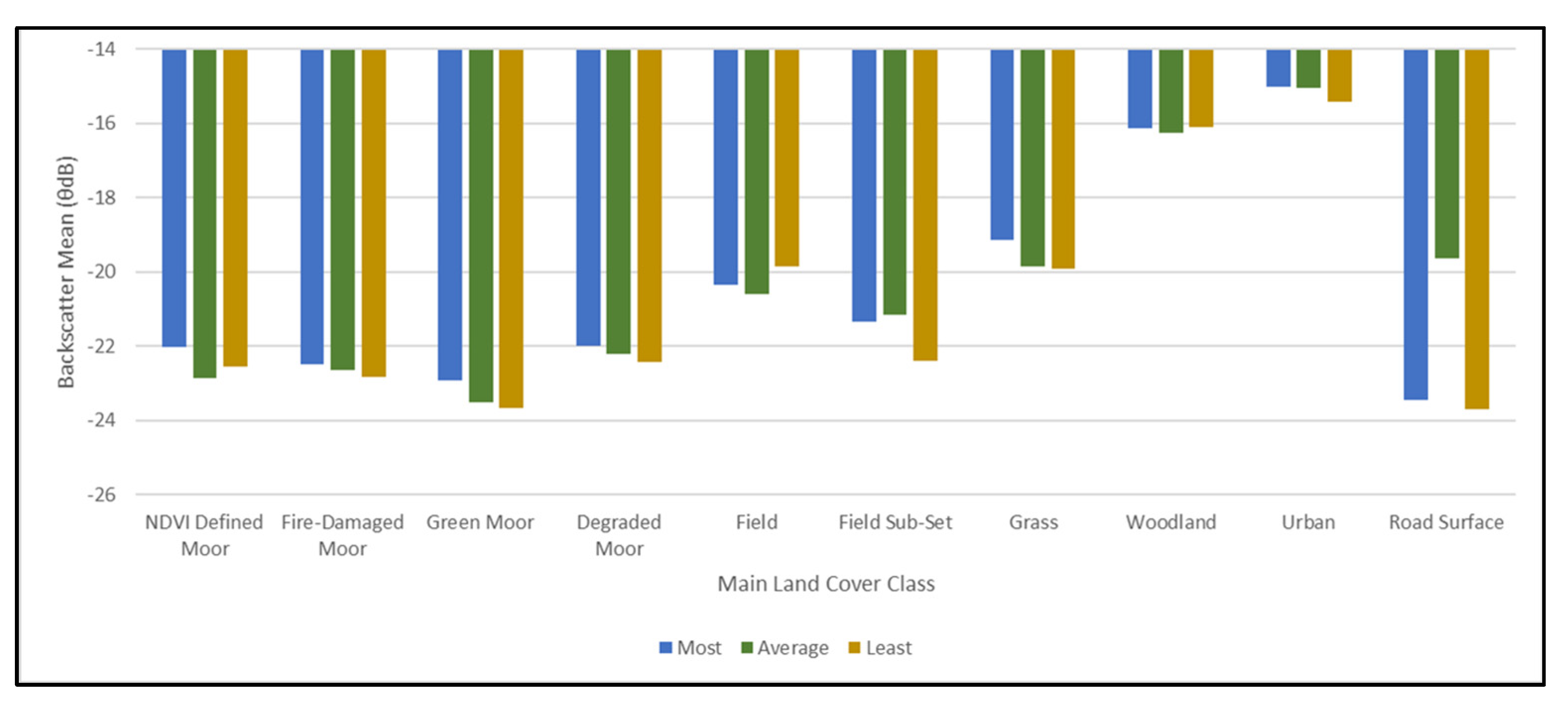
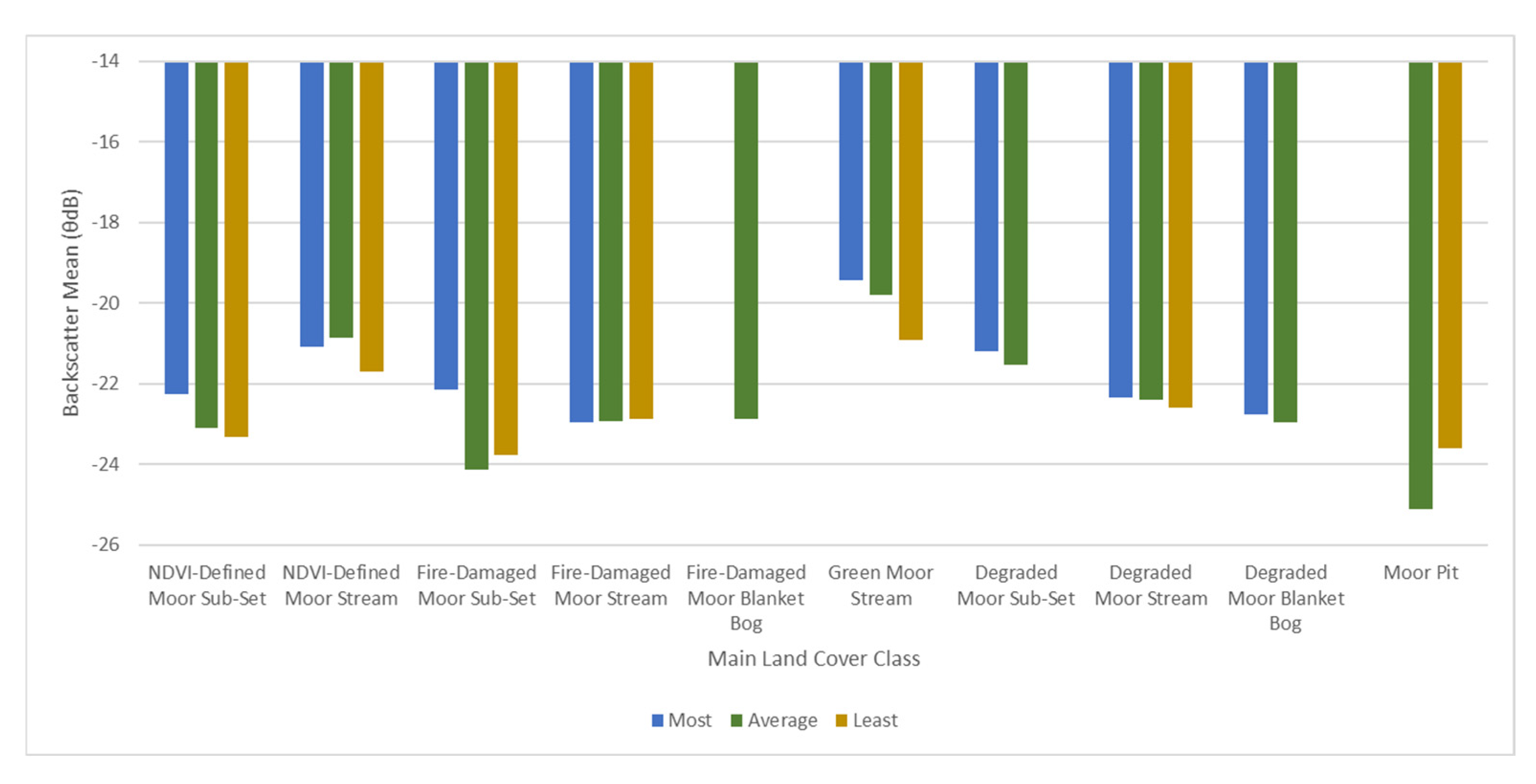
In assessing the effect of the hydrological function of each land cover sample, Figure 14 demonstrated a weak but noticeable pattern between TWI and backscatter across all the main peatland classes, which was replicated for the smaller peatland samples in Figure 15. This concurs with the findings of other research [10], but does not differ from other land cover classes, such as the Grass sample. Use of TWI therefore confirmed the prevalence of higher backscatter, where there is greater propensity of a wetter surface in peatland areas, but did not particularly aid the refinement of a delineation approach.

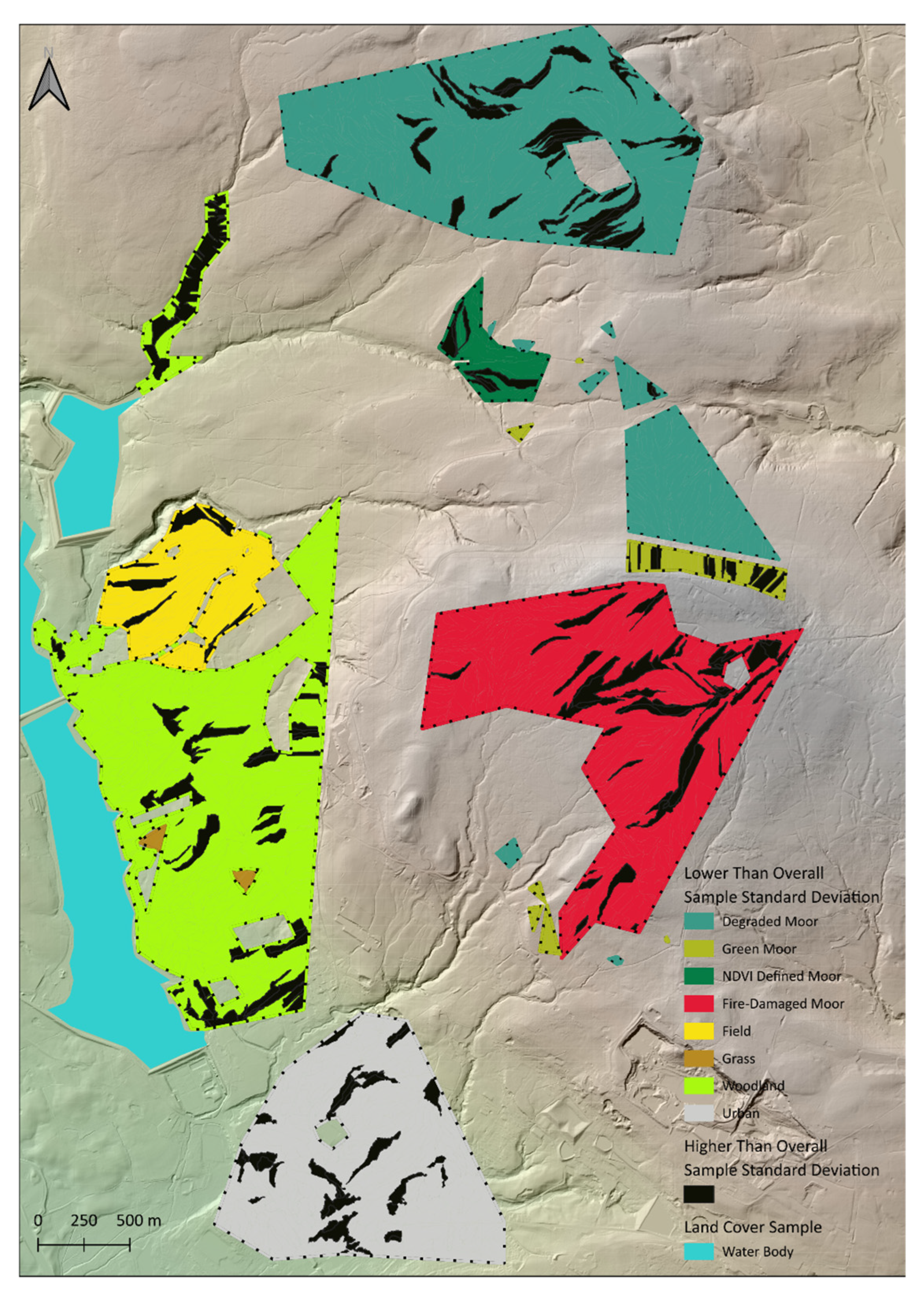
Still focusing on hydrology, but taking a different analytical approach, Figure 16 presents a sub-catchment perspective of the mean average Sentinel-1 backscatter within each land cover sample. Using the same parameters as Figure 7 to define relatively wet and dry peatland, backscatter data was contextualised at sub-catchment level, i.e., grouping the data into small hydrological regions. Figure 17 presents how this segmentation of backscatter generally resulted in a lower standard deviation of the data than the overall sample. Consequently, there is more concentrated distribution of most of the data when areas are segmented in this way. Potentially, this map provides a better understanding as to the variability of backscatter within each land cover sample. An example is the large Degraded Moor polygon (1d) in the north of each map, where in Figure 7 seemingly wetter areas are easy to observe, but dry, degraded peatland and areas more closely aligned with agricultural fields in terms of backscatter, are harder to delineate. On the other hand, Figure 16 provides more clarity as to the location of more acute degradation on the northern and eastern flanks of this sample. This is also the case for the Fire-Damaged Moor (1b), where peripheral degradation can be better observed in Figure 16.

4.6. Slope Influence on Delineation

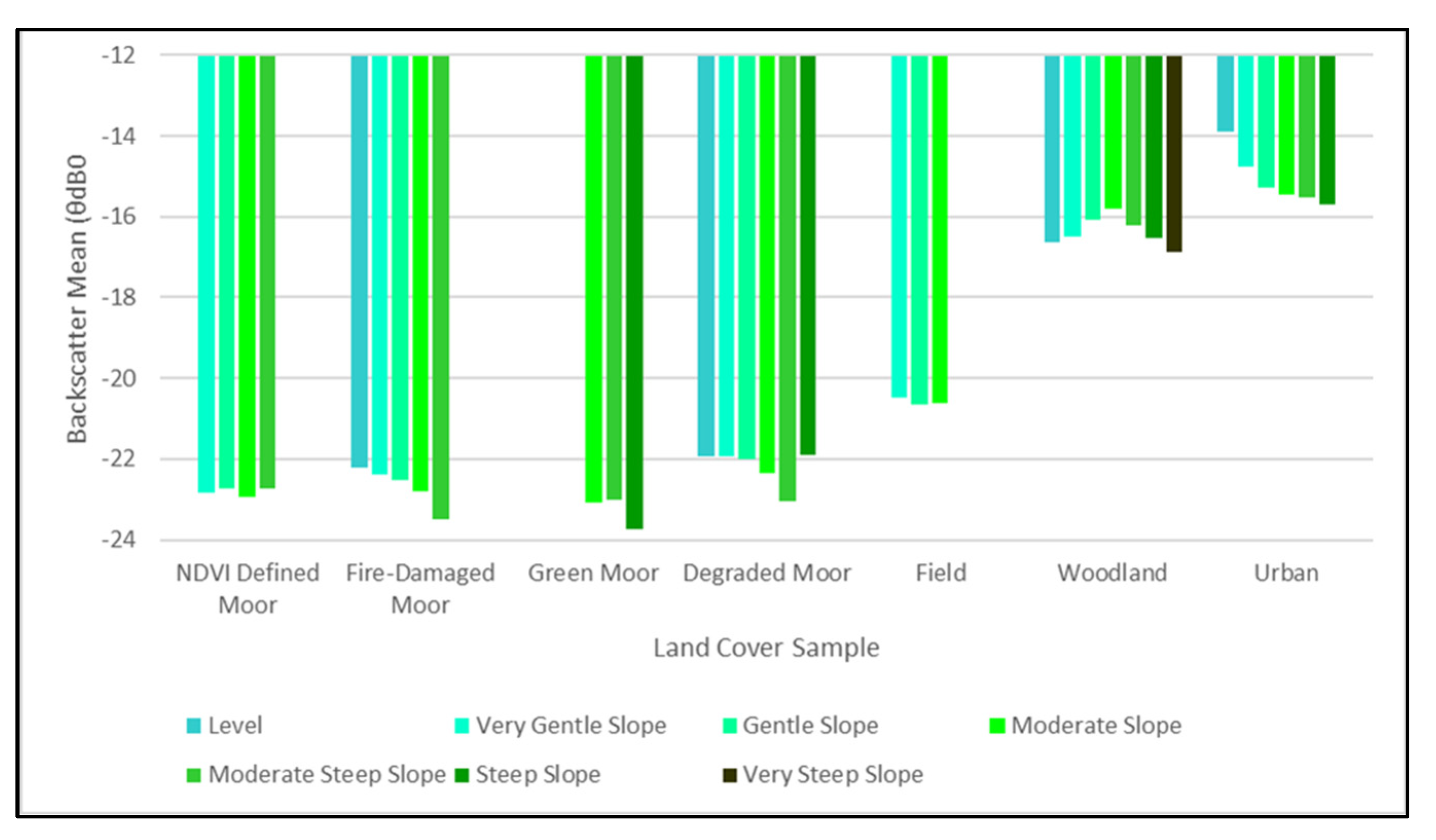
Better drainage on sloping surfaces within the moorland samples should, in theory, translate into higher backscatter in these locations. The effect of foreshadowing may also be a factor for all land cover samples where slope is most pronounced. Figure 18 demonstrates that generally backscatter decreases as slope increases. What is important in these findings is that where slope is most pronounced, this may be a significant factor affecting correlation of Sentinel-1 backscatter and temperature in frozen conditions. The Green Moor, Fire-Damaged Moor Sub-Set and Moor Pit samples were considerably steeper than other locations. The Green Moor had the lowest IQR of any land sample in frozen conditions and the two other samples had very low mean averages (Fire-Damaged Moor Sub-Set −23.96 θdB, Moor Pit −24.29 θdB). All three of these samples had almost no correlation between backscatter and temperature in frozen conditions. As demonstrated in Figure 10, when the steepest slopes were removed from the Green Moor sample, the relationship changed to a weak positive correlation. These findings therefore generally indicate some effect of slope, where most acute, in lowering backscatter for all land cover (excluding woodland as explained previously).

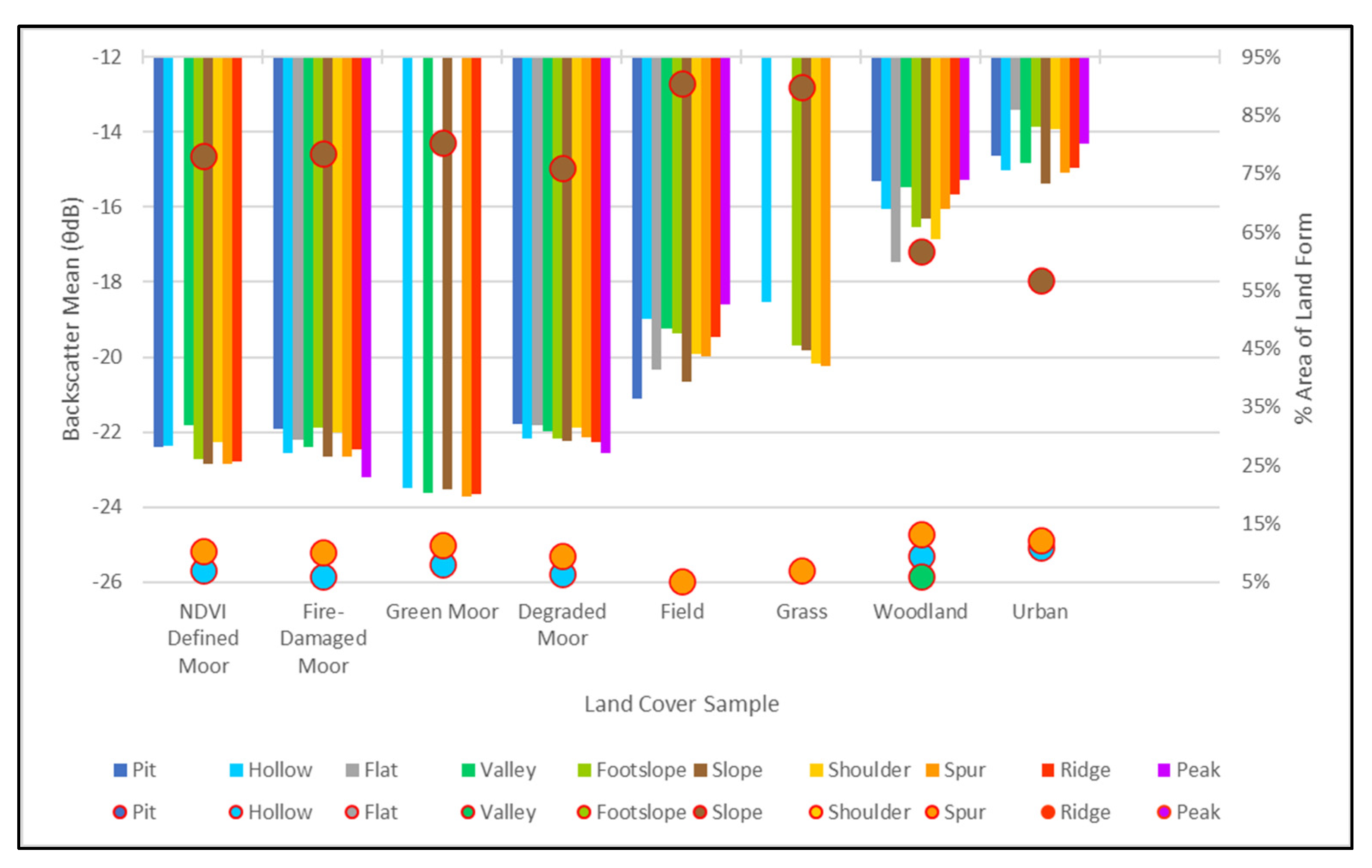
In Figure 19 topographic analysis of mean average Sentinel-1 backscatter in frozen conditions was further extended to landform features in each land cover sample. This also provided a view as to the prevalent landscape characteristics in each sample. For obvious reasons, water bodies were not included in this graph. The most common landform overall was sloping ground. Spurs were the next most common, but proportionally much less prevalent than sloping terrain. By order of general elevational position in a landscape, there was a detectable pattern for the peatland samples of backscatter decreasing from the depression features (pits and hollows) through to the highest features of ridges and peaks. The pattern was quite weak, but was noticeably different to the other land cover samples, where no real pattern emerged (aside from that of the Grass sample). Higher backscatter for pits and hollows was expected, as surrounding surfaces at a greater elevation may well proliferate a more intense radar response. However, lower backscatter on sloping ground and higher landform features contradicted what would be expected to happen, as these features had less or no water retention capabilities. Foreshadowing could be a contributing factor, but did not explain why this was not the case for the non-peatland samples. This finding does again support the notion that more acute terrain, where shoulders, spurs, ridges and peaks are more common landforms, results in lower backscatter response.

4.7. Optimal Peatland Delineation Methodology

Taking account of all the analysis conducted in this study, it is clear that the most distinguishable aspect of peatland in relation to Sentinel-1 backscatter signals is a consistently low return in frozen conditions compared with other land cover samples. When focusing solely on when snow cover has been verified, this correlation is not so clear. What is most important about this finding is how this differentiates peatland from grazed fields in the study cohort, as when conditions are warmer this distinction is much less prominent. Quite why this is the case is unclear. The obvious reason points to the water retention properties of peatland becoming more evident in these conditions. However, if this is the case then why did backscatter not easily correlate with segmentation by TWI, where water retention capabilities in relation to topography for each sample could be assessed in more detail? In fact, in the case of TWI, backscatter seemed to decrease in areas that had the least water retention capabilities. Further terrain analysis, as tested by slope and landform features, indicated that in the steepest areas, this correlation between temperature and backscatter for peatland in frozen conditions is weakest, probably due to the effect of foreshadowing.

Classification using thresholds derived from the IQR range of land cover samples does consistently represent general condition when using visual means of assessment, as demonstrated with the map/photograph comparisons in Figure 11. Segmenting this classification into hydrological regions, as the sub-catchment map in Figure 16, attempts to delineate not only peatland, but also the habitat’s condition in a more spatially coherent way. This has the potential to equip peatland habitat professionals with an alternative perspective to optical methods such as NDVI or NDMI and provide more detail in helping to assess this habitat at scale.

To augment this study, more Sentinel-1 datasets of the AOI in the same orbit pass when the temperature was below freezing need to be identified to further test statistical differences with agricultural fields in these conditions. A visual accuracy method has been the only assessment tool employed. Local stakeholder information from on-site monitoring on the extent of healthy and degraded peatland would be a valuable asset in further testing the accuracy of this delineation method. Surface roughness was not considered in this study as other research had found no real effect on backscatter. However, possible microtopographic effects specifically in peatland environments could be assessed using roughness indices in future research in this domain.

5. Conclusions

The use of Sentinel-1 SAR imagery in relation to peatland habitats has been proven in this study to highlight certain situations that may be worthwhile when assessing habitat extent, fire damage and relative condition. Sentinel-1 data has the advantages of consistent, regular coverage for even the most remote study areas and in any conditions.

The effects of fire damage are detectable using spectral imagery, but Sentinel-1 data can support current assessment techniques with consistent, ongoing monitoring activities that allows comparison with nearby similar habitat. Delineation of peatland surfaces from other land cover provides an approach that has the benefits highlighted above that may help more accurately map the extent of peatland habitat. Frozen conditions produce encouraging results in not only being able to delineate by land cover, but also in being able to provide an indication of relative wetness of a habitat. Whilst it is difficult to predict backscatter response in frozen conditions, especially where terrain is more challenging, these findings strongly indicate how further refinement has the potential to equip peatland practitioners with the ability to monitor habitat health at scale and more regularly.