Article

Spatiotemporal Mapping of Soil Profile Moisture in Oases in Arid Areas

1
College of Geography and Remote Sensing Science, Xinjiang University, Urumqi 830046, China
2
Xinjiang Institute of Technology, Aksu 843100, China
*
Author to whom correspondence should be addressed.
Remote Sens. 2025, 17(15), 2737; https://doi.org/10.3390/rs17152737 (registering DOI)
Submission received: 11 June 2025 / Revised: 1 August 2025 / Accepted: 4 August 2025 / Published: 7 August 2025
(This article belongs to the Section Remote Sensing in Geology, Geomorphology and Hydrology)

Abstract

Soil moisture is a key factor in the exchange of energy and matter between the soil and atmosphere, playing a vital role in the hydrological cycle and agricultural management. Traditional monitoring methods are limited in achieving large-scale, real-time observations, while deep learning offers new avenues to model the complex nonlinear relationships between spectral features and soil moisture content. This study focuses on the Wei-Ku Oasis in Xinjiang, using multi-source remote sensing data (Landsat series and Sentinel-1) and in situ multi-layer soil moisture measurements. The BOSS feature selection algorithm was applied to construct 46 feature parameters, including vegetation indices, soil indices, and microwave indices, and to identify optimal variable sets for each depth. Convolutional Neural Network (CNN), Long Short-Term Memory (LSTM), and their hybrid model (CNN-LSTM) were used to build soil moisture inversion models at various depths. Their performances were systematically compared on both training and testing sets, and the optimal model was used for spatiotemporal mapping. The results show that the CNN-LSTM-based multi-depth soil moisture inversion model achieved superior performance, with the 0–10 cm model showing the highest accuracy and a testing R2 of 0.64, outperforming individual models. The testing R2 values for the soil moisture inversion models at depths of 10–20 cm, 20–40 cm, and 40–60 cm were 0.59, 0.54, and 0.59, respectively. According to the mapping results, soil moisture in the 0–60 cm profile of the Wei-Ku Oasis exhibited a vertical gradient, increasing with depth. Spatially, soil moisture was higher in the central oasis and lower toward the periphery, forming a “center-high, edge-low” pattern. This study provides a high-accuracy method for multi-layer soil moisture remote sensing in arid regions, offering valuable data support for oasis water resource management and precision irrigation planning.

1. Introduction

Soil moisture content (SMC) refers to the amount of water in the soil that can be directly absorbed and utilized by plants [1]. It is a key parameter linking the surface water cycle and energy cycle, and accurately obtaining this parameter is crucial for understanding climate change, surface hydrological processes, and the mechanisms of land–atmosphere energy exchange [2]. Particularly in arid and semi-arid regions, agriculture is highly susceptible to drought stress, while soil moisture provides favorable conditions for sustained plant growth. It serves as a primary limiting factor for vegetation recovery and ecological restoration, exerting a more critical influence on plants than single rainfall events. In particular, deep soil moisture determines the amount of water available to plant roots [3]. Its dynamic trends are closely related to environmental protection, agricultural production, and disaster monitoring and early warning. Therefore, understanding the spatiotemporal moisture in arid and semi-arid regions is of great significance for assessing regional wetness and dryness conditions, ecosystem health, agricultural drought early warning, and optimized allocation of water resources.
Although traditional soil moisture monitoring methods such as the gravimetric method, resistance probe method, time domain reflectometry (TDR), and capacitance method are commonly used [4,5], these methods are relatively reliable in terms of accuracy, but their practical application is often limited by small spatial coverage, cumbersome operations, and high monitoring costs, making them unsuitable for large-scale, long-term monitoring. Remote sensing, with its advantages of wide-area and periodic observation, provides essential data support for estimating soil moisture at the regional scale [6,7]. Based on the data source, remote sensing for soil moisture monitoring is mainly categorized into microwave, optical, infrared and thermal infrared data. These two types employ different imaging mechanisms to characterize surface soil moisture from multiple dimensions. Microwave remote sensing, with its all-weather, all-day, and strong penetration capabilities, plays a crucial role in soil moisture retrieval. High spatiotemporal resolution data that are not affected by atmospheric interference are essential for accurate soil moisture monitoring [8,9]. Among Synthetic Aperture Radar (SAR) data sources, the Sentinel-1 satellite offers significant advantages due to its wide spatiotemporal coverage, moderate cloud penetration capability, and strong resilience under adverse weather conditions [10,11,12]. Optical remote sensing satellites (e.g., Landsat-8) provide 30 m resolution multispectral data, which are useful for deriving vegetation indices and hydrothermal parameters [12,13], but they are susceptible to atmospheric disturbances like clouds and rainfall, and their capacity to retrieve soil moisture under vegetative cover is relatively constrained [14]. Due to the limitations of individual sensors in spatial resolution, temporal coverage, and observation accuracy, relying solely on a single type of data is insufficient to comprehensively characterize the spatiotemporal distribution of soil moisture. Therefore, developing soil moisture prediction models that leverage multi-source data, achieve high accuracy, offer strong interpretability, and possess robust generalization capabilities has become a critical research focus in recent years. The integration of multi-source data enables the comprehensive utilization of observations from different platforms and modalities, facilitating data complementation and synergistic advantages, thereby significantly improving the accuracy and spatiotemporal adaptability of soil moisture retrieval.
Accurate and efficient soil moisture monitoring and prediction have become critical technological pathways for ensuring sustainable agriculture, effective water resource management, and good ecosystem stability. Traditional statistical regression methods face numerous challenges in soil moisture modeling, particularly when dealing with multi-source, multi-scale, and highly nonlinear remote sensing data, which often limits their modeling capability and adaptability [15]. With the increasing dimensionality and complexity of remote sensing data, the integration of high-dimensional, multi-source features introduces issues such as reduced modeling efficiency and the proliferation of redundant variables [16,17]. Consequently, feature selection algorithms are increasingly employed to enhance model performance. Common selection methods include Pearson’s correlation [18], SPA [19], and CARS [20]. The BOSS algorithm, based on bootstrap sampling and soft shrinkage, can iteratively evaluate the contribution of feature subsets to model performance. It effectively eliminates redundancy and multicollinearity without assuming variable distributions, showing strong performance in data preprocessing. Meanwhile, with the rapid development of machine learning, researchers are able to build more accurate and robust soil moisture prediction models even under conditions of limited or missing data [21,22]. Traditional machine learning algorithms such as Support Vector Machine (SVM) and Random Forest (RF) have been widely used for soil moisture estimation, achieving promising results [23]. For example, Duan et al. [24] used Landsat 8 thermal and optical sensors to retrieve soil moisture by applying various machine learning algorithms such as RF, SVM, artificial neural networks (ANNs), and elastic net regression (EN), and the results showed that RF performed best in predicting soil moisture under test conditions. Building on this, research gradually shifted toward deep learning architectures, which significantly improved the accuracy and efficiency of soil moisture modeling. For example, Fan et al. [25] constructed a fused feature set using Sentinel-1 and GF-6 data in the Shihezi Oasis of Xinjiang, comparing the performance of CNN, RF, and other models for cotton field soil moisture estimation. Their results showed that the CNN model outperformed the other methods across multiple accuracy metrics. Wang et al. [26] explored the potential of attention-based neural networks for soil moisture prediction. Their results showed that the Transformer model achieved an average R2 of 0.523 under various time lags, outperforming the LSTM model with an R2 of 0.485. The incorporation of LSTM enhanced the stability of the Transformer in modeling temporal variations. Roberts et al. [27] integrated surface reflectance features using a CNN to enhance GNSS-R soil moisture retrieval accuracy. Although soil moisture inversion studies have made significant progress, most research remains focused on surface soil moisture. Deep and multi-layer moisture retrievals have received limited attention and are often confined to small-scale areas. For instance, Wu et al. [28] estimated soil moisture in citrus orchards using multimodal UAV remote sensing. Li et al. [29] studied kiwifruit orchards in Meixian County, using UAV and ground sensors to collect vegetation spectral reflectance and soil moisture data. They developed a BiLSTM model for root-zone soil moisture inversion, achieving a test R2 of 0.62 and RMSE of 2.45%, offering theoretical support for water management in other orchards. However, multi-layer soil moisture (e.g., 0–60 cm) is a key water source for plant root uptake and surface evapotranspiration, and its dynamic variations more accurately reflect vegetation responses to water stress. High-precision, multi-depth soil moisture monitoring is vital for understanding ecosystem responses and optimizing irrigation regulation in arid regions. Therefore, achieving synergistic inversion of multi-layer soil moisture within deep learning frameworks remains a key challenge and frontier in current soil moisture remote sensing research.
Based on this, this study takes the typical oasis in arid regions—Wei-Ku Oasis—as the study area, aiming to construct a multi-layer soil moisture inversion framework integrating multi-source remote sensing data and deep learning methods, in order to provide a theoretical basis and technical support for agricultural water resource management and ecosystem regulation in oasis areas. The specific objectives of this study are as follows: (1) to construct a multitemporal fused feature set based on Landsat series optical remote sensing data and Sentinel-1 SAR data, including vegetation indices, spectral indices, and radar polarization features; (2) to apply the Bootstrapping Soft Shrinkage (BOSS) feature selection algorithm to achieve adaptive screening of optimal variable combinations for different soil layers (0–10 cm, 10–20 cm, 20–40 cm, and 40–60 cm); (3) to using Convolutional Neural Network (CNN), Long Short-Term Memory (LSTM), and hybrid CNN-LSTM models, and perform multi-layer soil moisture synergistic inversion based on multi-period in situ data from 2017 to 2024 in the Wei-Ku Oasis; (4) to evaluate the performance of different models and use the optimal model to conduct the spatial mapping of multi-layer soil moisture in the Wei-Ku Oasis, providing methodological support for water resource management and precision irrigation decision-making at the regional scale in arid regions.

2. Materials and Methods

2.1. Study Area

The Weigan River–Kuqa River Delta Oasis (hereinafter referred to as the Wei-Ku Oasis) is located in the Xinjiang Uygur Autonomous Region of China (Figure 1). It is bordered by the Tianshan Mountains to the north and the Taklamakan Desert to the east, situated geographically between 41°05′ and 41°45′N latitude and 82°10′ and 83°45′E longitude. The area is about 9000 square kilometers and characterized by a continental warm temperate hyper-arid climate [30]. Under the combined influence of persistent aridity and the interlaced mountain–basin geomorphological pattern, a typical and well-developed fan-shaped alluvial plain has evolved [31]. The regional climate features low precipitation and aridity, with an average annual temperature ranging from 10.5 to 15.4 °C, annual precipitation between 50.0 and 66.5 mm, and evapotranspiration reaching 1990 to 2865 mm, resulting in a dryness index of 42:1 [32]. Precipitation is scarce and unevenly distributed spatially, while evaporation is intense, classifying the area as a typical mid-latitude arid zone. The region has an average annual sunshine duration of 2884.43 h and an average frost-free period of 240 days per year. Due to the water distribution characteristics in the study area, vegetation in the Wei-Ku Oasis is primarily divided into two types: artificial vegetation in irrigated farmland within the oasis and natural vegetation in the desert–oasis transition zone at the oasis periphery [33]. Under the extremely arid desert climate conditions, natural vegetation types are sparse and structurally simple, mostly consisting of drought- and salt-tolerant desert plants. The dominant native vegetation includes Phragmites australis, Alhagi sparsifolia, and Karelinia caspica [34].

2.2. Data

2.2.1. Soil Moisture Data

Soil samples were collected in the field from June to July of 2017, 2018, 2021, 2022, and 2024 (Figure 2, Table 1). Soil moisture information was obtained through field surveys and experimental observations using the five-point sampling method. Soil samples were taken in the study area with ring cutters and aluminum boxes, and the latitude and longitude of sampling points were recorded using GPS 72 (Garmin Ltd., Olathe, KS, USA) devices. Sampling points were evenly distributed across cultivated land, transitional desert areas, and regions outside the oasis to ensure comprehensive spatial coverage. Soil samples were collected from soil layers at depths of 0–60 cm, with three replicates per layer. Samples were promptly sealed in aluminum boxes and weighed immediately using a precision electronic balance with 0.1 g accuracy to obtain fresh weight. In the laboratory, soil moisture content was determined using the oven-drying method, which yields gravimetric soil moisture content and has not been converted to volumetric content. The soil moisture calculation formula is as follows:
θ   =   ω 2     ω 3 ω 3     ω 1   ×   100 %
where θ represents gravimetric soil moisture content (%), ω 1 is the mass of the empty aluminum box (g), ω 2 is the mass of the aluminum box with wet soil (g), and ω 3 is the mass of the aluminum box with dry soil (g).

2.2.2. Remote Sensing Imagery Data

This study employed multitemporal Sentinel-1 and Landsat series sensors to acquire soil moisture parameters across different periods in the Wei-Ku Oasis region. The Landsat data consisted of 11 spectral bands, while the Sentinel-1 data included vertically (VV) and horizontally (VH) polarized backscatter, along with derived SAR indices. All satellite data were preprocessed using Google Earth Engine (GEE). The preprocessing of Landsat data involved radiometric calibration, atmospheric correction, and image clipping. For Sentinel-1, the preprocessing steps included data ingestion, multi-look processing, filtering, radiometric calibration, geocoding, normalization, and clipping. The final outputs comprised atmospherically corrected spectral bands, VV and VH backscatter coefficients, and composite SAR indices. Due to limitations such as cloud cover and imaging intervals, remote sensing images cannot be strictly aligned with the sampling times of each ground point. Therefore, this study selected the closest time windows during the same period across multiple years, with remote sensing data covering June to July from 2017 to 2024.

2.3. Methods

2.3.1. Index Construction

Due to the complex surface structure of the Wei-Ku Oasis, relying solely on a single sensor for soil moisture retrieval has inherent limitations in both spatial and temporal dimensions. Integrating the strengths of multiple sensor types has become a research hotspot for improving soil moisture inversion. In this study, various indices were constructed based on optical, thermal, and microwave polarization parameters, as well as those commonly used in previous studies, using data from different sensors, as summarized in Table 2. Optical indices included the Normalized Difference Vegetation Index (NDVI), Enhanced Vegetation Index (EVI), and Soil-Adjusted Vegetation Index (SAVI), while radar-based indices involved vertical transmit and vertical receive (VV) and vertical transmit and horizontal receive (VH). A total of 46 feature parameters were selected for analysis.

2.3.2. Bootstrap Soft Shrinkage Algorithm

The Bootstrap Soft Shrinkage (BOSS) [59] algorithm is a variable selection optimization method that integrates bootstrap sampling (BSS) and weighted bootstrap sampling (WBS) to generate the final subset of variables. Bootstrap sampling is a non-parametric resampling technique that generates multiple training subsets by performing sampling with replacement on the original dataset, allowing the assessment of variable importance and stability across different samples. Weighted bootstrap sampling further incorporates sample weights, increasing the probability of selecting certain samples, thereby guiding the model to focus more on key variables or samples. It is widely used in high-dimensional data analysis and regression tasks, especially in the fields of spectral data analysis and machine learning model optimization. The goal of BOSS is to identify important features through multiple resampling iterations and a soft shrinkage strategy, which helps to minimize multicollinearity and enhance model generalization and predictive performance. Its core idea combines bootstrap resampling, bias control, and sparsity processing to ensure that the selected feature subset is both representative and capable of effectively reducing model complexity [60].

2.3.3. Models

(1) Convolutional Neural Network
Convolutional Neural Networks (CNNs) are predominantly employed in image recognition and computer vision tasks [61]. The fundamental concept behind CNNs lies in their ability to extract complex image features through the use of convolutional layers, pooling layers, and fully connected layers [62,63]. Typically, a CNN model consists of convolutional layers, activation functions, pooling layers, and fully connected layers, with convolutional layers forming its core. These layers apply convolution operations to the input images, effectively capturing local features and generating corresponding feature maps. Convolutional kernels with different parameters produce multi-dimensional feature maps that capture hierarchical information within the images. Nonlinear activation layers (such as ReLU, Sigmoid, Tanh) apply thresholding to feature maps, enhancing the model’s ability to represent complex functional relationships. Pooling layers reduce the spatial dimensions of the feature maps through operations like max pooling or average pooling while preserving critical features. Finally, fully connected layers convert the dimensionally reduced feature matrices into feature vectors and perform the final prediction through fully connected mappings. In this study, the CNN regression model primarily consists of convolutional layers and fully connected layers, designed to extract spatial features from input data and perform regression prediction. The architecture includes two convolutional layers and three fully connected layers, with nonlinear mapping implemented via the ReLU activation function.
(2) Long Short-Term Memory
Long Short-Term Memory (LSTM), a variant of a Recurrent Neural Network (RNN), is specifically designed for processing sequential time series data. Compared with traditional RNNs, LSTM demonstrates enhanced memory capabilities by employing gating mechanisms that significantly improve the modeling of long-term dependencies and effectively alleviate common training issues such as vanishing and exploding gradients [64,65]. The core computational units of LSTM comprise three gates: The input gate controls the degree to which new information updates the cell state. The forget gate regulates the influence of the previous cell state on the current step. The output gate determines how much of the cell state is exposed to the external output, thus enabling hierarchical modeling of complex temporal relationships [66,67]. In this study, the LSTM model adopts a two-layer LSTM architecture, with each layer containing 64 hidden units. This configuration effectively captures long-term dependencies within the input sequences. Temporal features are extracted through the LSTM layers and subsequently fed into fully connected layers for regression prediction. The mathematical expressions of each gate in the LSTM model are as follows:
I t   =   δ ω i · G h t 1 , x t   +   b f
F t = δ ω f · G h t 1 , x t + b f
O t =   δ ω 0 · G h t 1 , x t + b 0
G t =   t a n h ω g · G h t 1 , x t + b g
ω = ω h t 1 , ω x t
h t = O t · tanh C t
C t = F t C t 1 + I t G t
Here, I , F , O , and G represent the input gate, forget gate, output gate, and cell state, respectively, h denotes the hidden state, C stands for the cell state, x is the input, δ represents the activation function, b indicates the bias for each gate, ω corresponds to the weights of each gate, and t denotes the time step.
(3) CNN-LSTM
The CNN-LSTM model is a deep learning architecture that combines Convolutional Neural Networks (CNNs) and Long Short-Term Memory networks (LSTM) to simultaneously process spatial (e.g., images) and temporal sequence data. CNNs effectively extract spatial correlation features from input data through convolutional operations. This architecture plays a crucial role in characterizing one-dimensional time series signals, especially excelling at uncovering latent local patterns within the data. In contrast, LSTMs introduce memory cells and gating mechanisms to build a deep temporal modeling framework for sequential data. Their unique forget/input/output gate collaboration not only accurately captures dynamic dependencies across time steps but also effectively models long-range dependencies during data evolution [68]. Typically, the CNN-LSTM model consists of CNN layers followed by LSTM layers. Input data first pass through convolutional layers to extract local spatial features, which are then modeled temporally by the LSTM layers. This design provides significant advantages in handling spatiotemporal data such as image sequences and has achieved promising results in various prediction tasks [69]. In our soil moisture prediction task, the CNN-LSTM model consists of convolutional and LSTM layers. Initially, two one-dimensional convolutional layers followed by pooling operations are used to extract local features. These features are then passed to an LSTM layer with 50 hidden units to capture temporal dependencies, and finally, the regression output is produced through three fully connected layers.

2.3.4. Model Evaluation

To evaluate the accuracy of each model, three statistical metrics were employed: the coefficient of determination (R2), mean absolute error (MAE), and root mean square error (RMSE). The R2 metric represents the proportion of variance in the observed data explained by the model, while RMSE measures the prediction accuracy of the model. MAE quantifies the average magnitude of errors in the model’s predictions, providing an intuitive measure of overall prediction error. A higher R2 value closer to 1 indicates better model fit, whereas lower RMSE and MAE values signify improved model performance. The calculation formulas for these evaluation metrics are as follows:
R 2   =   k = 1 n Y k , m     Y ¯ k , m Y k , e     Y ¯ k , e 2 k = 1 n Y k , m     Y ¯ k , m 2 k = 1 n Y k , e     Y ¯ k , e 2
M A E = 1 n k = 1 n Y k , m   Y ¯ k , e
R M S E = 1 n k = 1 n Y k , m Y k , e 2
where Y k , m , Y k , e and Y ¯ k , m represent the measured soil moisture values, model-predicted values, and number of observations, respectively.

3. Results

3.1. Descriptive Statistics of Measured Sample Data

The descriptive statistics of soil characteristics at different depths of the measured sampling points are shown in Table 3. Soil moisture content in the study area varies considerably. At a 0–10 cm depth, SMC ranges from 0.43% to 30.47%, with an average of 10.60% and a coefficient of variation (CV) of 60.29%; at 10–20 cm, from 1.23% to 28.43%, with a mean value of 14.31%; at 20–40 cm, from 0.81% to 37.91%, averaging 14.76%; and at 40–60 cm, from 1.18% to 34.80%, with a mean of 15.78%. Overall, the mean gravimetric soil moisture content in the Wei-Ku Oasis shows an increasing trend with depth, increasing from 10.60% to 15.78%. The coefficient of variation for soil moisture at each layer exceeds 30%, indicating strong spatial variability. The possible causes of this high variability include the following: first, the differences in vegetation cover, where areas with dense vegetation have higher demand for soil moisture and nutrients, while areas with sparse cover are more directly exposed to intense solar radiation; second, pronounced human activities in the study area, such as the continuous expansion of newly cultivated farmland and abandoned land, which severely disrupt soil structure, resulting in significant variability in soil moisture.

3.2. Multi-Layer Feature Variable Selection

This study employed the BOSS feature selection algorithm to screen feature variables. The maximum number of latent variables was set to 15, and the number of bootstrap samples was set to 1000. By repeatedly sampling and variable selection to optimize the model, the feature variables that contributed most to model performance were ultimately selected. The 46 feature variables were screened using the BOSS algorithm separately for soil layers at depths of 0–10 cm, 10–20 cm, 20–40 cm, and 40–60 cm. The types of selected features at different depths included vegetation indices, band reflectance, soil indices, and polarization indices, comprehensively considering the importance of various factors in model construction. The specific selected variable combinations are shown in Table 4.

3.3. Construction and Comparison of Soil Moisture Retrieval Models

Using the measured sample data and the optimal variable combinations selected for each soil layer, models were built to compare the predicted soil moisture content with the observed values. This study evaluated the performance of three deep learning models in soil moisture prediction. The soil moisture samples from the Wei-Ku Oasis region were divided into training and testing datasets, with 70% and 30% of the samples, respectively. To optimize the model architecture and parameter settings, multiple rounds of structural combination tests were conducted on the training set. The tests covered hidden unit numbers, convolution kernel sizes, number of LSTM layers, and learning rate. The final structure with the best overall performance on the validation set, based on R2, RMSE, and MAE, was selected as the final parameter configuration for each model. The parameter settings used in each model are listed in Table 5.
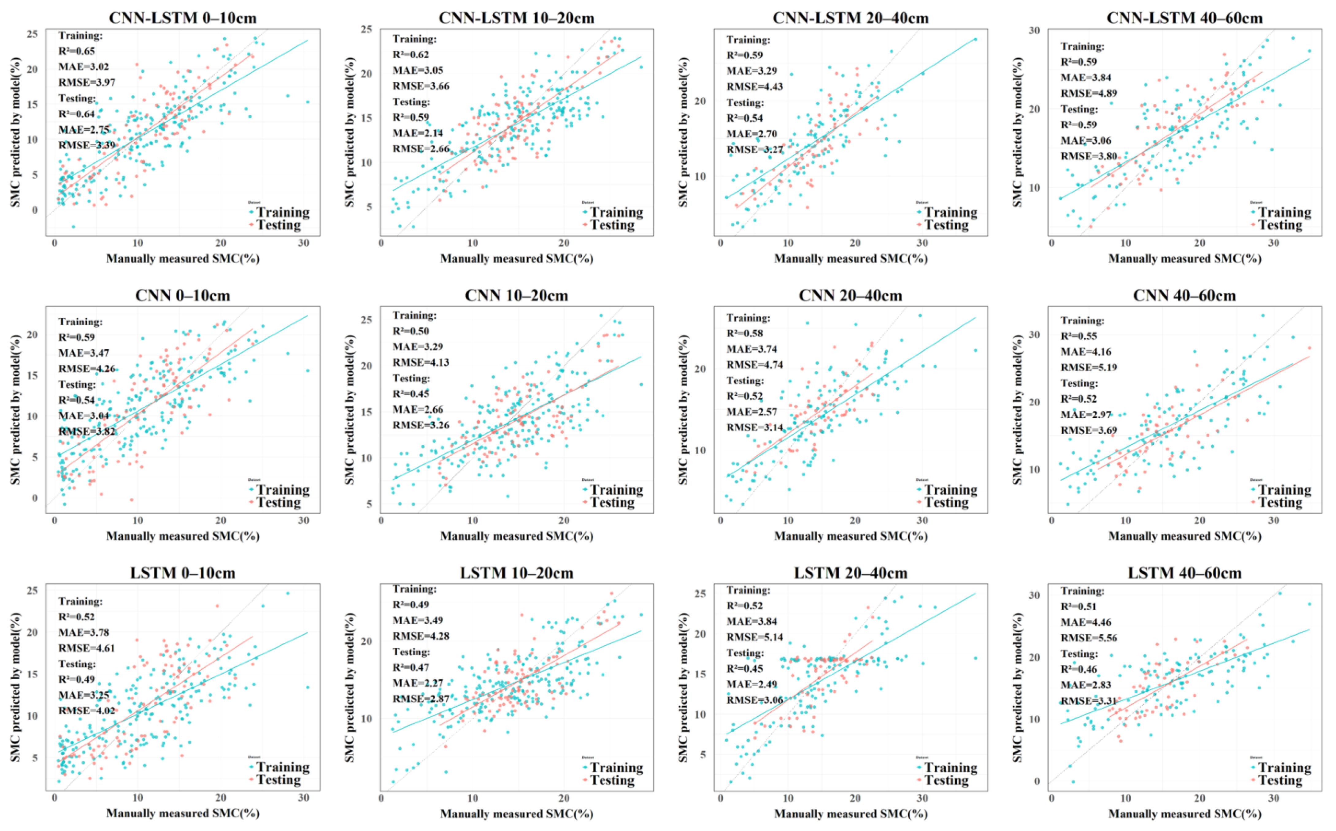
Figure 3 shows the accuracy validation of soil moisture inversion models at different depths, where the comparison between observed and predicted values illustrates the prediction accuracy of the CNN-LSTM model. Table 6 present the R2, MAE, and RMSE values for the training and testing sets of each model at soil depths of 0–10 cm, 10–20 cm, 20–40 cm, and 40–60 cm. Considering the performance across all models and datasets, the model accuracies are ranked as follows from highest to lowest: CNN-LSTM, CNN, and LSTM. The CNN-LSTM model consistently achieved the highest R2 values in soil moisture prediction across different depths, confirming the advantage of the hybrid model in integrating spatiotemporal features. At the 0–10 cm depth, CNN-LSTM showed the best performance (testing set R2 = 0.64, MAE = 2.75%, RMSE = 3.39%), followed by CNN (R2 = 0.54), with LSTM performing the worst (R2 = 0.49). CNN’s performance at the surface layer (0–20 cm) was close to that of CNN-LSTM, but its errors increased at greater depths (>20 cm). Although LSTM exhibited the weakest overall performance, its testing set MAE and RMSE at 20–40 cm and 40–60 cm depths were slightly better than those of the other models despite having the lowest R2. This suggests that deeper soil moisture is likely influenced by long-term processes such as infiltration and transpiration; thus, LSTM’s temporal feature modeling offers better generalization for deep soil moisture. All models showed an increasing trend in error from surface to deeper layers (e.g., CNN-LSTM’s RMSE increased from 3.37% to 3.80%), which is consistent with the physical principle of diminishing remote sensing signal penetration. However, the LSTM model’s MAE at the depth of 20–40 cm (2.49%) was lower than that at the surface, possibly because mid-layer soil moisture correlates more strongly with meteorological time series data such as precipitation.

3.4. Soil Moisture Mapping

3.4.1. Soil Moisture Mapping at Different Depths

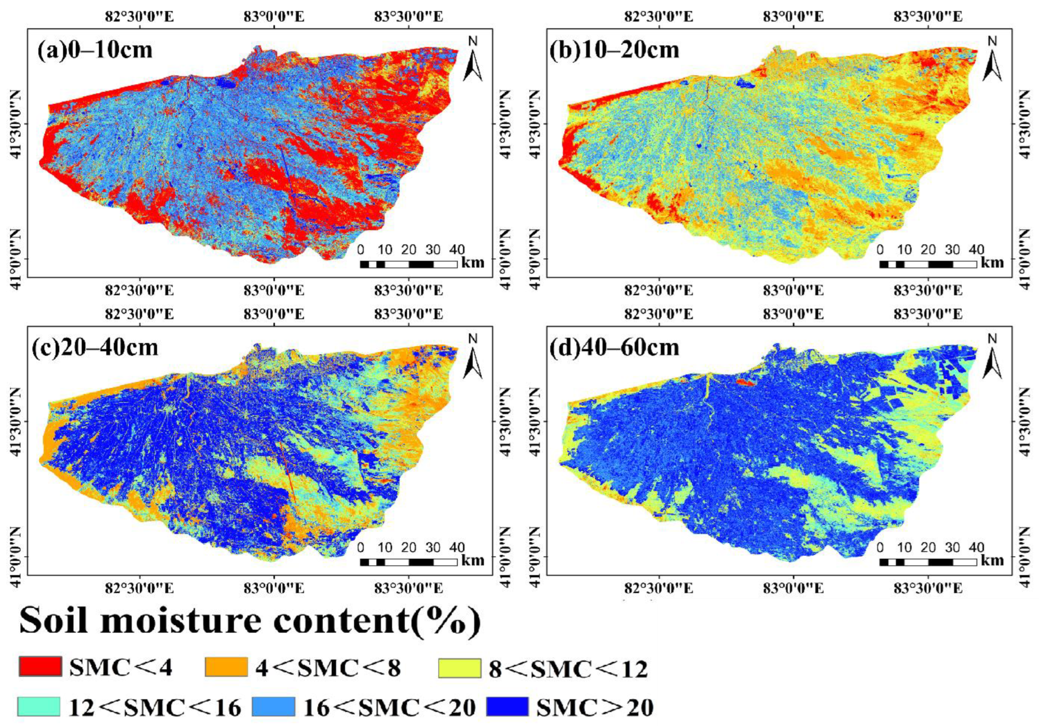
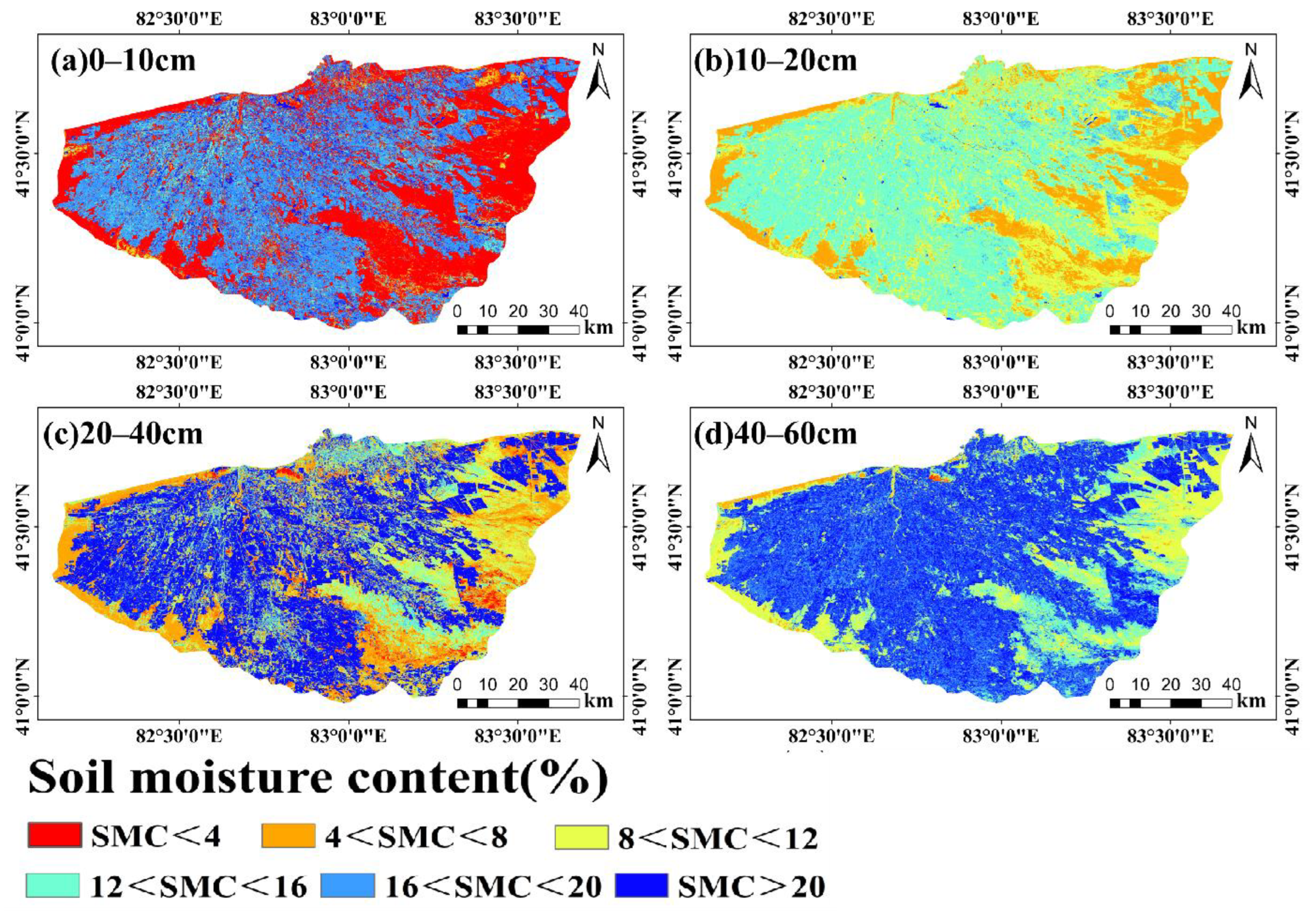
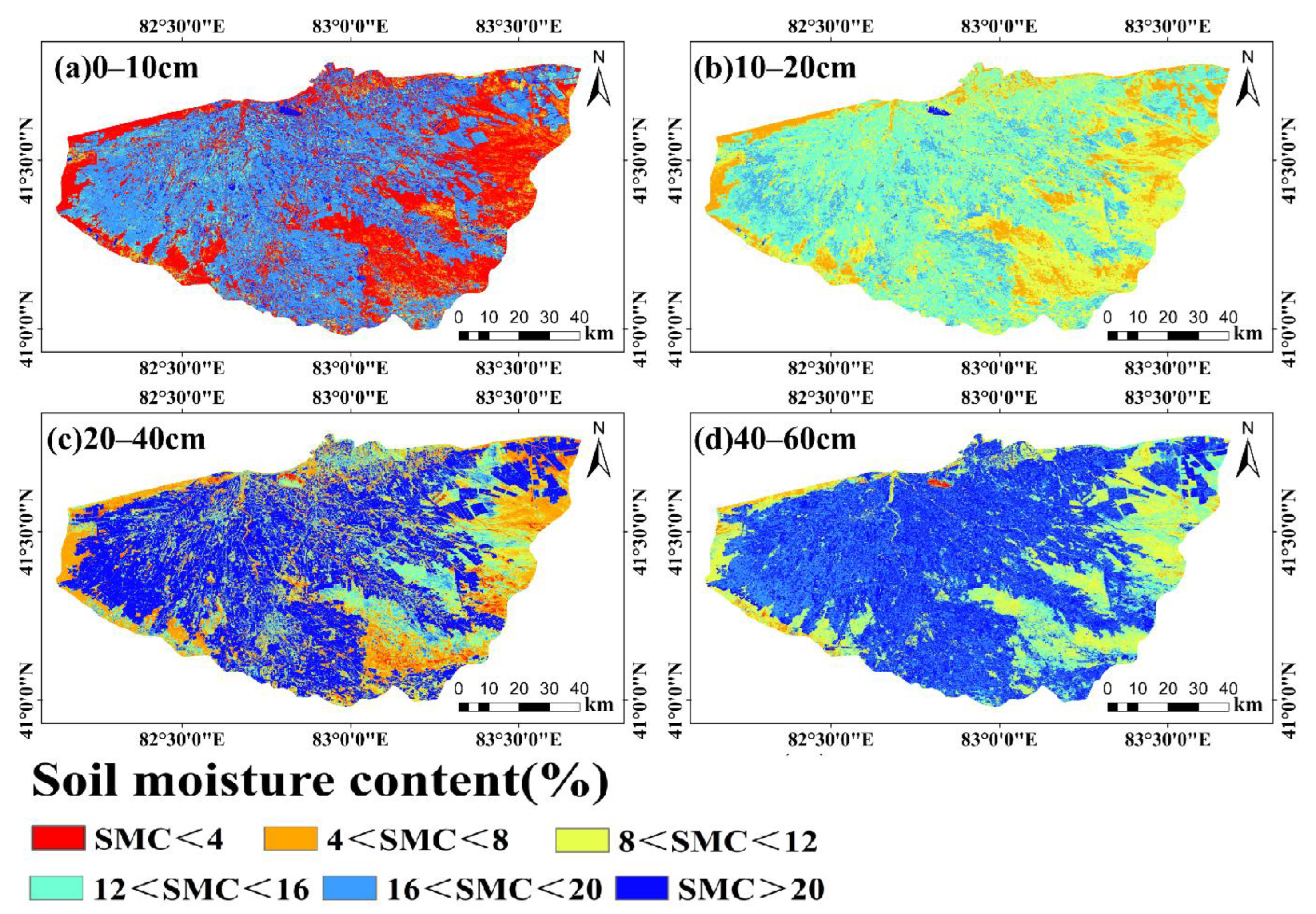
Based on the results above, soil moisture was mapped using the CNN-LSTM model and remote sensing imagery, producing spatial distribution maps of soil moisture at different depths (0–10 cm, 10–20 cm, 20–40 cm, and 40–60 cm) for the years 2017 to 2024 (see Appendix A Figure A4, Figure A5, Figure A6, Figure A7, Figure A8, Figure A9 and Figure A10). Taking 2024 as an example (Figure 4), the average soil moisture content at each depth was 11.69% (0–10 cm), 12.12% (10–20 cm), 15.91% (20–40 cm), and 18.96% (40–60 cm), showing an increasing trend with soil depth. This result is highly consistent with the descriptive statistical analysis of measured sample data in Section 3.1, indicating stronger water retention capacity in deeper soils and demonstrating the reliability of the model’s predictions.
The shallow surface layer (0–10 cm) is significantly influenced by meteorological factors (e.g., rainfall and evaporation) and surface cover types (e.g., vegetation). Areas with high soil moisture are mainly found in regions with good vegetation coverage and irrigated zones within oases, whereas lower soil moisture is observed in bare land or sandy soil areas, typically located at the oasis margins. The middle soil layer (10–40 cm) serves as a key transitional zone for soil water migration. It exhibits more moderate moisture levels and less variability than the surface layer, receiving both downward infiltration from precipitation or irrigation and upward fluxes via water vapor or capillary rise. The 20–40 cm layer is wetter than the 10–20 cm layer, especially in irrigated regions, where it shows a stronger water-holding capacity. Deep soil (40–60 cm) has the highest moisture content and the lowest overall variability. This is partly because it experiences the least evaporative loss, and partly due to the slow accumulation of capillary water and deep infiltration, resulting in a relatively high and stable moisture level.

3.4.2. Soil Moisture Mapping Across Different Years

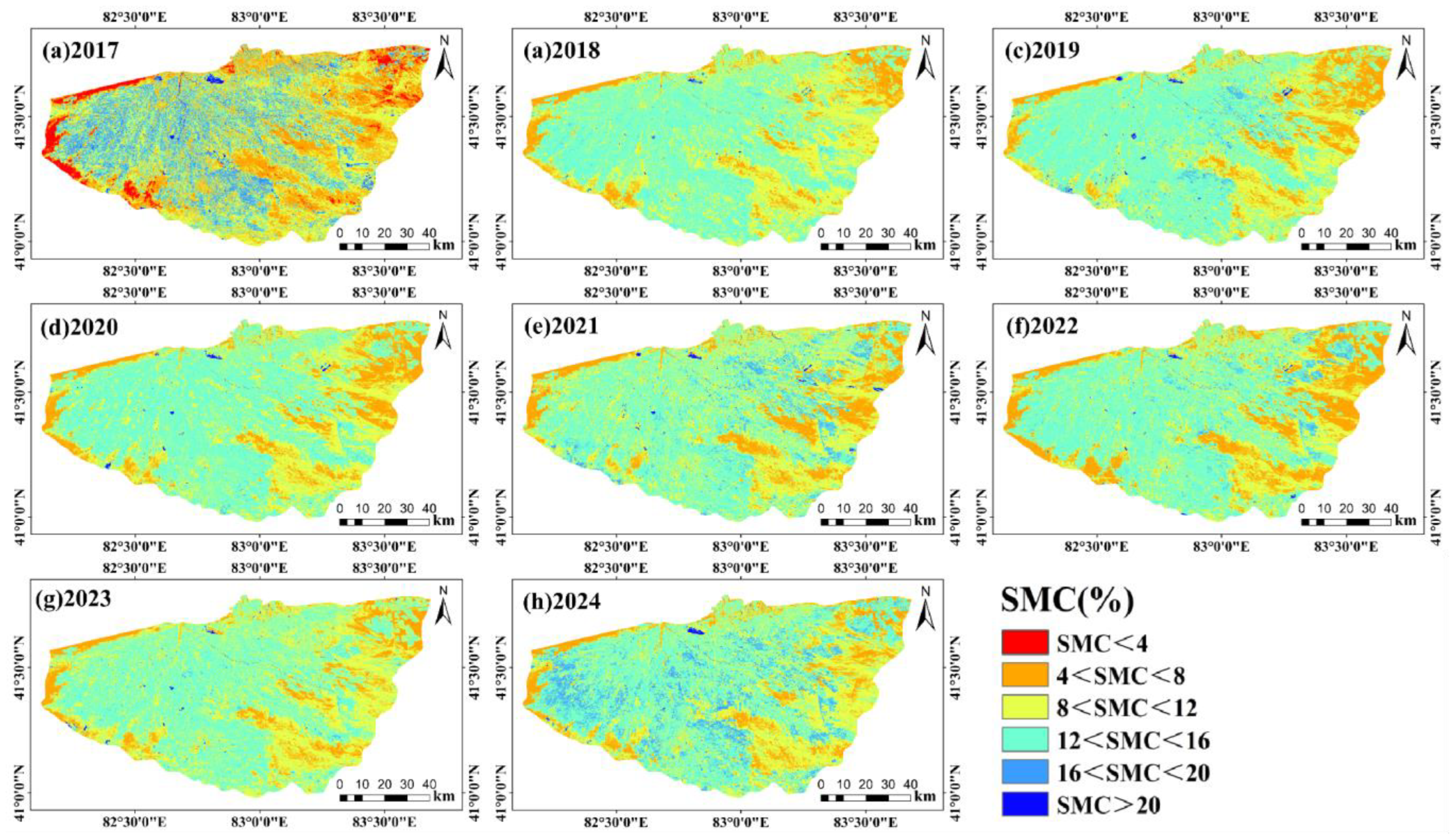
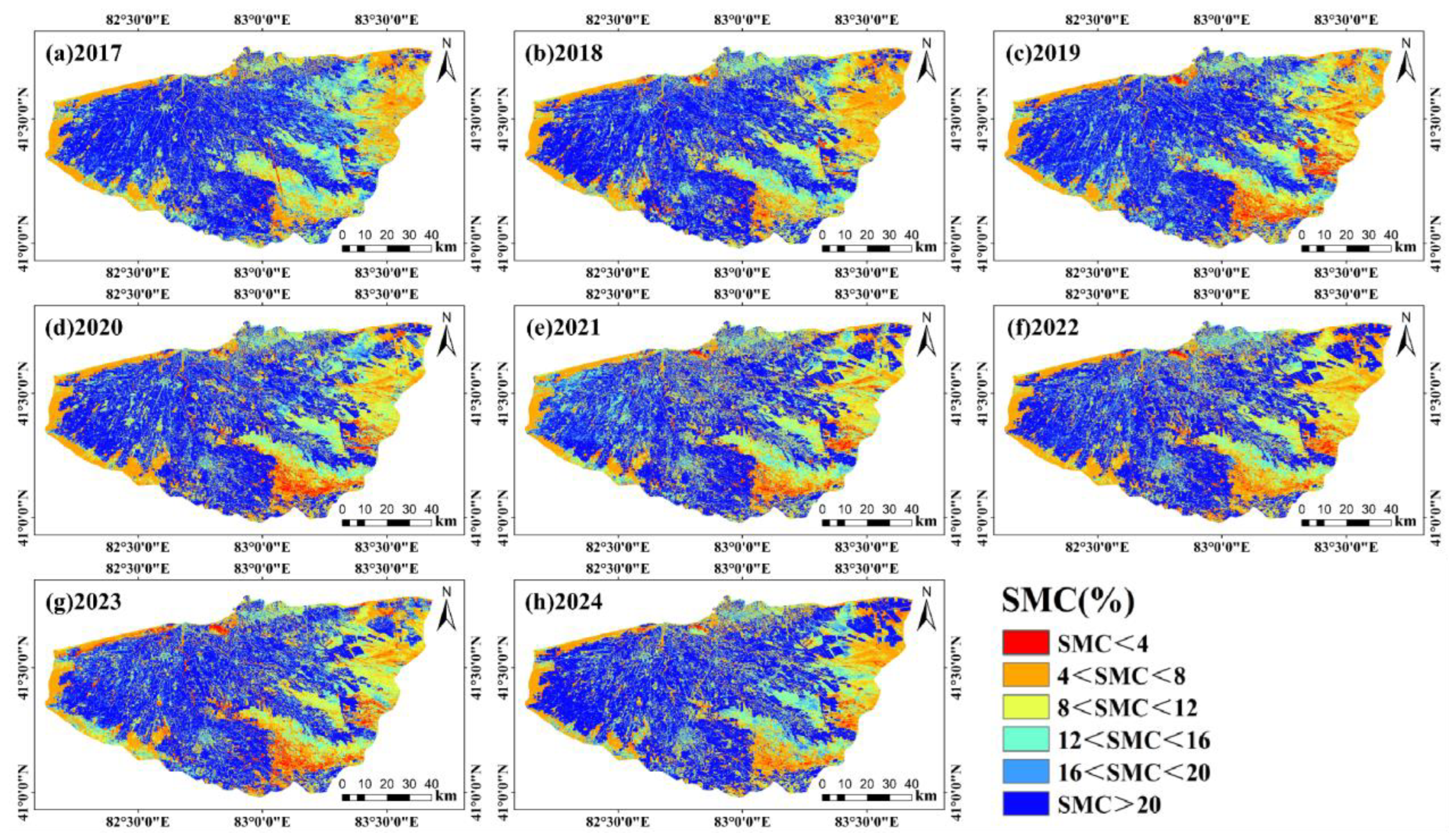
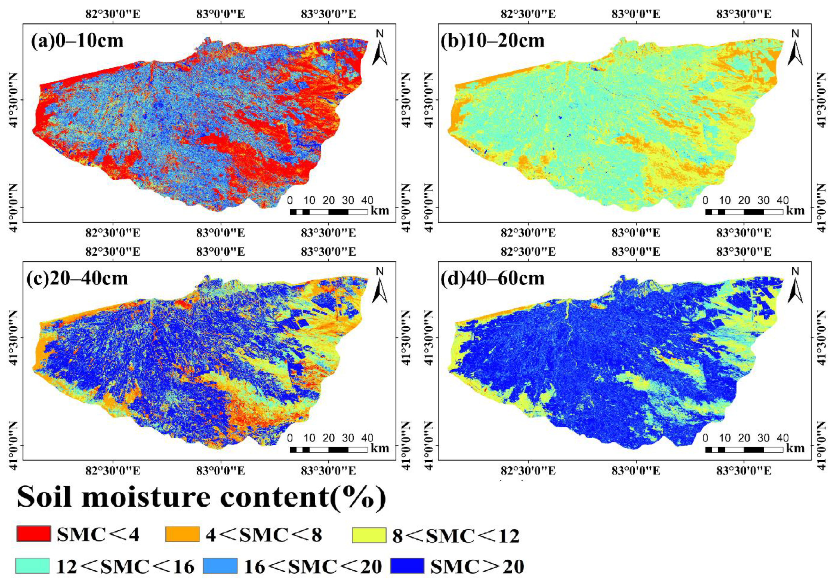
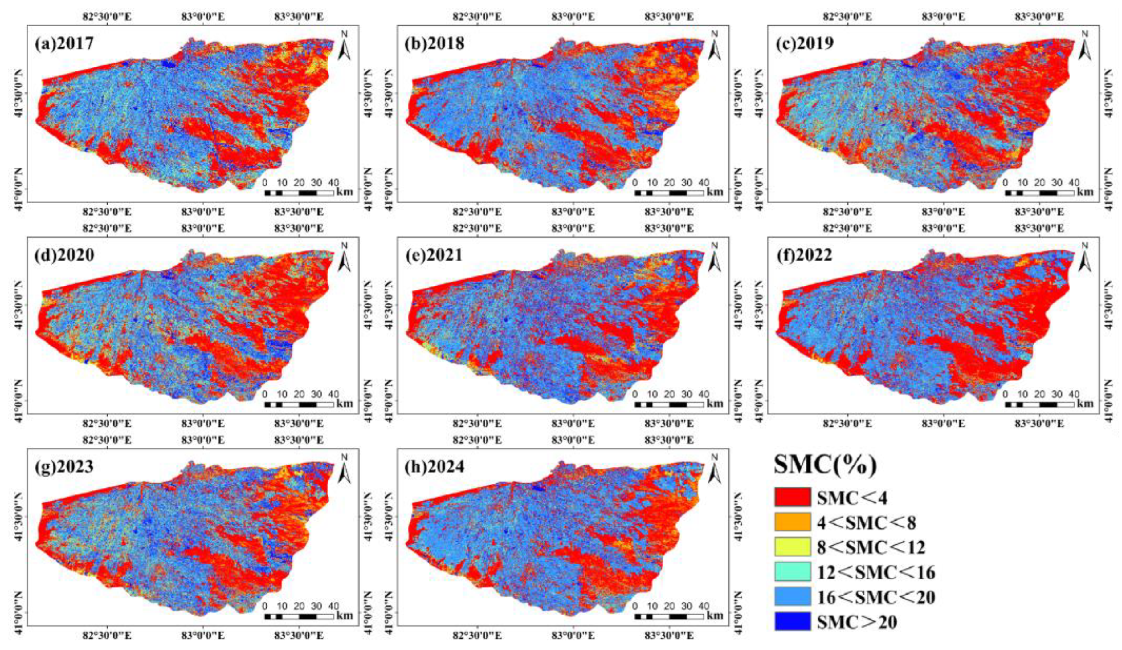
The CNN-LSTM model was used to map soil moisture and obtain the spatial distribution of soil moisture at different depths each year (see Appendix A Figure A1, Figure A2 and Figure A3). Taking Figure 5 as an example, the spatial distribution characteristics of soil moisture in Wei-Ku Oasis in 2024 are analyzed. In June and July, rising temperatures and strong evaporation characterize the study area. Although precipitation increases during this period, the oasis functions as a typical irrigated agricultural zone with frequent artificial water supply and dense vegetation cover, resulting in strong soil water retention.
Consequently, soil moisture within the oasis is significantly higher than in surrounding areas, with an average content of approximately 11%. Specifically, the Weigan and Kuqa River basins and the surrounding reservoir areas are significantly affected by water supply, with relatively high soil moisture levels and the formation of localized “high-moisture patches,” indicating the important role of surface water in soil moisture replenishment. In contrast, soil moisture content in the desert–oasis transition zone is significantly lower, exhibiting pronounced spatial fragmentation and heterogeneity. This region is dominated by sandy soils with loose structure, high porosity, and poor water retention. Combined with long-term wind erosion and arid climatic conditions, the soils are prone to moisture loss, resulting in a “low-moisture zone.” Additionally, the western edge of the region has lower gravimetric soil moisture content compared to the eastern edge. This can be attributed to its location in an arid zone with minimal natural water coverage, where the land surface is largely bare or sparsely vegetated, experiencing intense evaporation and severe salt accumulation, which exacerbates soil aridification. Overall, the spatial distribution of soil moisture within the Wei-Ku Oasis is relatively uniform and high, while the surrounding transitional zones exhibit low moisture content and strong heterogeneity. The pronounced moisture gradient along the oasis–desert boundary reflects the significant influence of regional ecological conditions and land use practices on soil moisture distribution.
Secondly, from 2017 to 2024, the overall spatial distribution of soil moisture remained consistent, exhibiting a pattern of “high in the center and low at the margins,” reflecting stable irrigation conditions and soil structure in the region. However, compared with previous years, the northeastern part of the study area showed a gradual increase in soil moisture in 2024, which may be attributed to farmland reclamation activities in the region. Conversely, slight decreases in soil moisture were detected in some southeastern areas of the study region, potentially influenced by land use changes. Furthermore, the spatial pattern observed in this study—higher soil moisture in the oasis center and lower moisture in the surrounding desert—is the result of multiple interacting environmental factors. Specifically, regional climate conditions (e.g., high temperature, intense evaporation, uneven precipitation), soil physicochemical properties (such as texture, porosity, and organic matter content), and land use practices (including cropland concentration, irrigation intensity, and vegetation cover) collectively shape the spatial distribution of soil moisture. The farmland areas within the oasis retain more moisture due to continuous irrigation and vegetation cover, whereas the surrounding desert zones experience rapid moisture loss owing to intense evaporation, high permeability, and poor water-holding capacity. Additionally, salt crusting caused by the high salinization in the Wei-Ku Oasis further inhibits water infiltration, exacerbating soil moisture gradients. Overall, the CNN-LSTM model demonstrates strong inversion accuracy and effectively captures spatial variations in soil moisture at the regional scale, indicating robust generalization performance.

4. Discussion

4.1. Selection of Feature Parameters

The feature variables used for modeling soil moisture at various depths, selected based on the BOSS (Bootstrapped Adaptive Sparse Sampling) algorithm, included spectral indices derived from original bands, vegetation indices, water indices, and tasseled cap transformations. These variables formed diverse combinations for model construction. The reflectance characteristics associated with soil moisture directly capture spatial variations in surface water content. Vegetation spectral indices affected by soil moisture stress can serve as indirect indicators of regional water status. Particularly in remote sensing inversion models, these indices effectively reveal the coupling between soil moisture and vegetation physiological responses in vegetated areas [70]. Moisture indices hold unique value in monitoring soil moisture conditions in arid regions, as they can characterize surface moisture dynamics in sparsely vegetated zones such as desert transition areas, and also assess water surplus and deficit conditions in irrigated oasis farmlands [71]. Soil indices derived from the ratio of red-edge bands (e.g., Landsat-8 B5) to shortwave infrared (SWIR) bands (B6/B7) can be used to infer soil particle size and surface roughness, which in turn affect water infiltration rates (e.g., soils with higher roughness tend to exhibit greater water retention capacity). Sentinel-1 radar data provide penetrative backscatter information, enhancing the detection of soil surface and shallow moisture and indirectly reflecting deeper soil moisture through vegetation–soil coupling effects [72,73]. Additionally, improved water indices and the wetness component derived from the tasseled cap transformation offer critical spectral indicators for large-scale soil moisture mapping. The BOSS algorithm was selected in this study for feature variable selection, primarily due to its soft shrinkage modeling mechanism, which allows it to retain key features that consistently perform well across most subsamples while compressing regression coefficients. This effectively reduces the risk of overfitting in the presence of multicollinearity [74,75]. In recent years, BOSS has been widely applied in high-dimensional spectral modeling and environmental parameter retrieval. Studies have shown that regression models built using BOSS exhibit high accuracy in feature selection and strong modeling performance. Zhang et al. [34] applied BOSS to variable selection for soil salinity prediction, improving model precision. Li et al. [76] found that BOSS enabled better prediction performance in modeling soil organic matter and total nitrogen with fewer selected wavenumbers and shorter computation time. These studies demonstrate that BOSS, as a robust and efficient feature selection method, can optimize model input structure and enhance both generalization and computational efficiency.

4.2. Performance Evaluation of CNN, LSTM, and CNN-LSTM Models

It is worth noting that although remote sensing data, such as from Sentinel-1 and Landsat, are physically limited in penetration depth and cannot directly observe soil moisture below 10 cm, this study did not aim to physically retrieve deep-layer moisture using remote sensing. Instead, remote sensing features were used as input variables, combined with in situ soil moisture observations, to construct a deep learning-driven spatial modeling framework. This approach focuses on the mapping relationships between features and the model’s generalization ability, representing a typical data-driven modeling strategy widely applied in regional-scale soil moisture estimation and remote sensing inversion tasks [77,78,79].
The results demonstrate that the hybrid CNN-LSTM architecture exhibits the best predictive performance, outperforming the standalone LSTM and CNN models. As a foundational model, the Convolutional Neural Network effectively compresses network parameters during feature extraction through its inherent weight-sharing mechanism. This not only simplifies model complexity but also significantly enhances the system’s robustness against noise. However, it should be noted that the traditional CNN architecture is primarily suited for processing static spatial features and has inherent limitations in capturing dynamic temporal dependencies in sequential data, particularly for long-term sequence relationships [80,81]. Compared to CNN, LSTM performs better in time series modeling by introducing cell states and gating mechanisms, enabling the effective modeling of long-term temporal dependencies [82,83,84]. However, in this study’s multi-layer soil moisture spatial inversion task, which focuses on short-term spatial mapping with limited temporal information, the temporal modeling capability of LSTM cannot be fully utilized. Due to its strong spatial feature extraction ability, flexibility in multi-source data fusion, and advantage in producing high-resolution outputs, the CNN model performs better than LSTM [85]. In this study, a CNN-LSTM hybrid model was constructed through an architecture fusion strategy aimed at integrating the complementary strengths of both models: leveraging CNN’s spatial feature extraction capability and LSTM’s temporal modeling advantage. This hybrid model can better learn and fit network layers of the model structure [86], achieving higher prediction accuracy compared to the standalone LSTM and CNN models. However, other studies have indicated that hybrid models do not always improve accuracy over the original models. Possible reasons for this include the following [87,88,89]: On the one hand, independent models coupled to find an optimal solution may converge to local optima, and inappropriate parameter combinations can weaken model performance, resulting in accuracy that is not satisfactory compared to the original models. On the other hand, prediction accuracy is related to the user’s experience with the model; differences in parameter tuning expertise among users can lead to variability in results, with experienced users being more likely to approach optimized outcomes. According to our results, the CNN-LSTM model significantly outperforms the independent models in prediction accuracy, providing a robust methodological support for intelligent irrigation decision-making at the regional scale.

4.3. Limitations and Future Prospects

Soil moisture is influenced by many factors such as vegetation cover, water infiltration, runoff, evaporation, and soil surface characteristics, making the accurate simulation of its spatial variation critically important. In specific regions, the effects of topography and physical parameters on soil moisture can be somewhat mitigated based on land use. The hybrid model proposed in this study considers the advantages of different sensors and reflects physiological information of surface vegetation but does not take into account soil physical properties such as porosity, bulk density, and organic matter content. Future research will incorporate these soil physical parameters. Moreover, our soil moisture inversion relies on relevant spectral indices without considering environmental driving factors like topography, climate, and soil properties. Integrating these environmental factors into soil moisture inversion models could improve prediction accuracy and represents a key direction for future studies. Although multiple feature variables based on radar and optical data were used, many potentially valuable variables remain unexplored. Future work can consider incorporating additional features that contribute more significantly to model inversion accuracy. However, increasing the number of features also increases model complexity; thus, complexity penalties such as the Bayesian Information Criterion (BIC) can be applied to balance model performance and complexity. For deeper soil moisture prediction, integrating low-frequency remote sensing data (e.g., L-band) or groundwater measurements may enhance inversion accuracy at depth. Due to limitations in the structure and quantity of sampling data, this study independently estimated soil moisture at different depths to capture the spatial variation patterns at specific layers across the oasis region, rather than simulating the vertical continuity of the soil moisture profile. Future research will explore modeling frameworks that consider inter-layer associations, such as multi-output neural networks, multi-task learning models, or deep spatiotemporal collaborative modeling, to improve physical consistency and structural coherence across soil profiles. Additionally, the satellite monitoring of soil moisture in this region faces challenges due to widespread salinization in arid areas, where surface roughness and salt crust heterogeneity induce directional spectral anisotropy, complicating accurate remote sensing. Therefore, multi-angle and multitemporal satellite observations can help reduce interference effects and improve soil moisture inversion in desert soils. This approach is expected to become a key focus in arid-zone soil moisture monitoring research.

5. Conclusions

This study employed three deep learning models—Convolutional Neural Network (CNN), Long Short-Term Memory (LSTM), and their hybrid model (CNN-LSTM)—along with the BOSS feature selection algorithm to predict soil moisture at different depths in the Wei-Ku Oasis using multitemporal Landsat series and Sentinel-1 remote sensing data. The spatiotemporal prediction of soil moisture within 0–60 cm depth provides crucial data support for large-scale intelligent irrigation decision-making. The results indicate that the CNN-LSTM framework achieved the best overall performance and accuracy for multi-depth soil moisture inversion, followed by the CNN and LSTM models. The CNN-LSTM model achieved testing R2 values of 0.64, 0.59, 0.54, and 0.59 at depths of 0–10 cm, 10–20 cm, 20–40 cm, and 40–60 cm, respectively, outperforming the single models at all layers. According to the soil moisture maps generated by the CNN-LSTM model, all soil layers from 0 to 60 cm in the Wei-Ku Oasis exhibited a clear vertical moisture gradient, with moisture increasing with depth. Spatially, soil moisture in the oasis interior was significantly higher than in the surrounding desert margins, forming an overall distribution pattern of higher values in the center and lower values at the periphery.

Author Contributions

Conceptualization, Z.Z. and J.W.; methodology, Z.Z. and J.Z.; software, Z.Z. and L.S.; validation, Z.Z.; formal analysis, Z.Z. and J.W.; investigation, Z.Z.; resources, J.W.; data curation, Z.Z., J.W. and J.D.; writing—original draft preparation, Z.Z.; writing—review and editing, J.W., J.Z., L.L., L.S. and Y.L.; visualization, Z.Z. and L.L.; supervision, J.W.; project administration, J.W. and J.D.; funding acquisition, J.W. and J.D. All authors have read and agreed to the published version of the manuscript.

Funding

This study was funded by the Innovative Team for Efficient Utilization of Water Resources in Arid Regions (NO.2022TSYCTD0001) and the Survey of Meteorological Elements in the Tuha Basin (No.: 202134120009).

Data Availability Statement

The data are available on request to the first author.

Conflicts of Interest

The authors declare no conflicts of interest.

Abbreviations

The following abbreviations are used in this manuscript:
CNNConvolutional Neural Networks
LSTMLong Short-Term Memory networks
SMCSoil moisture content
BOSSBootstrap Soft Shrinkage Algorithm

Appendix A

Appendix A.1

Figure A1. Soil moisture distribution map at a depth of 10–20 cm in Wei-Ku Oasis from 2017 to 2024.
Remotesensing 17 02737 g0a1
Figure A2. Soil moisture distribution map at a depth of 20–40 cm in Wei-Ku Oasis from 2017 to 2024.
Remotesensing 17 02737 g0a2
Figure A3. Soil moisture distribution map at a depth of 40–60 cm in Wei-Ku Oasis from 2017 to 2024.
Remotesensing 17 02737 g0a3
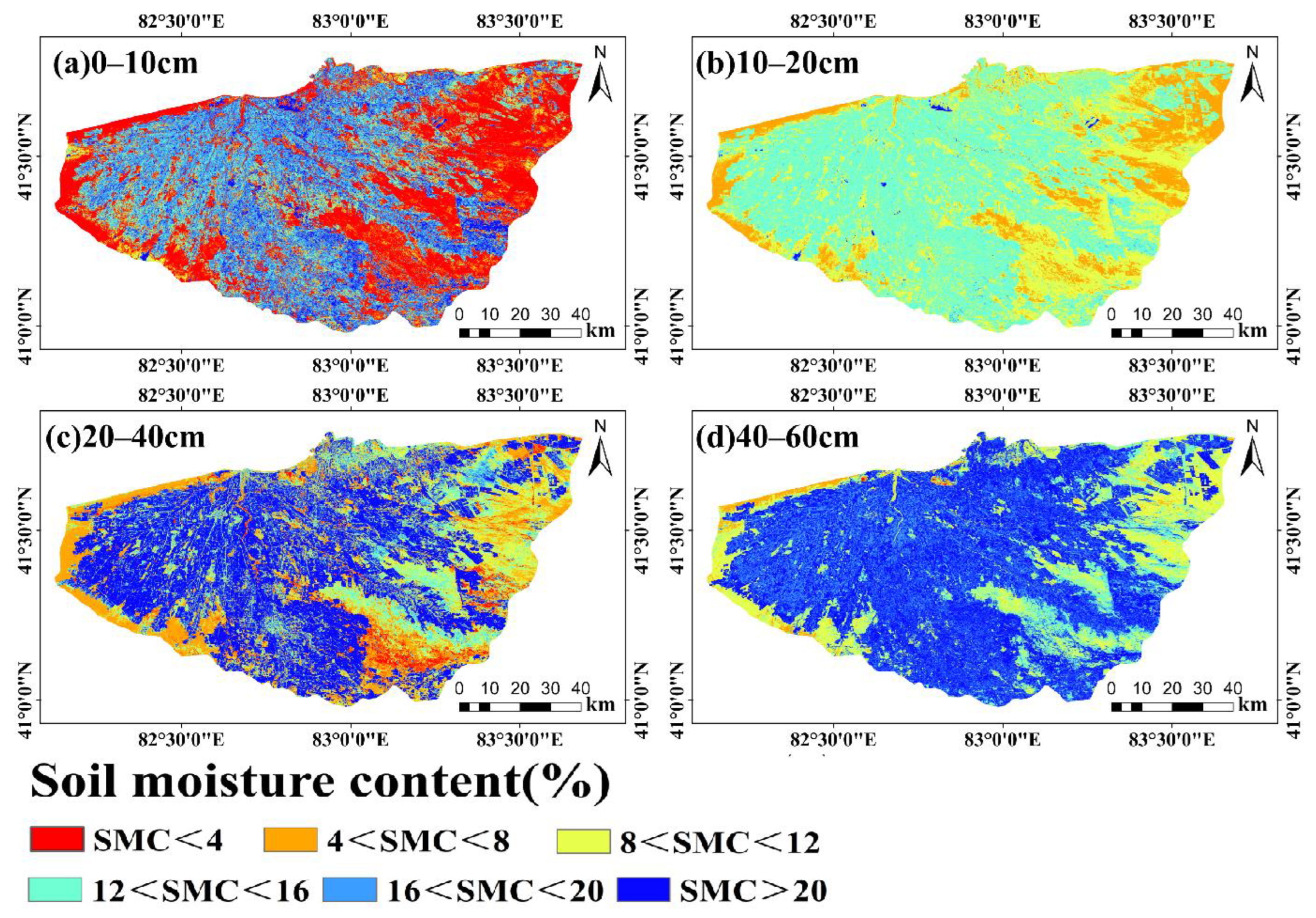
Figure A4. Spatial distribution of soil moisture at different depths in Wei-Ku Oasis in 2017.
Remotesensing 17 02737 g0a4
Figure A5. Spatial distribution of soil moisture at different depths in Wei-Ku Oasis in 2018.
Remotesensing 17 02737 g0a5
Figure A6. Spatial distribution of soil moisture at different depths in Wei-Ku Oasis in 2019.
Remotesensing 17 02737 g0a6
Figure A7. Spatial distribution of soil moisture at different depths in Wei-Ku Oasis in 2020.
Remotesensing 17 02737 g0a7
Figure A8. Spatial distribution of soil moisture at different depths in Wei-Ku Oasis in 2021.
Remotesensing 17 02737 g0a8
Figure A9. Spatial distribution of soil moisture at different depths in Wei-Ku Oasis in 2022.
Remotesensing 17 02737 g0a9
Figure A10. Spatial distribution of soil moisture at different depths in Wei-Ku Oasis in 2023.
Remotesensing 17 02737 g0a10

References

  1. Qin, X.; Pang, Z.; Jiang, W.; Feng, T.; Fu, J. Progress and development trend of soil moisture microwave remote sensing retrieval method. J. Geo-Inf. Sci 2021, 23, 1728–1742. [Google Scholar] [CrossRef]
  2. Ge, X.; Ding, J.; Jin, X.; Wang, J.; Chen, X.; Li, X.; Liu, J.; Xie, B. Estimating agricultural soil moisture content through UAV-based hyperspectral images in the arid region. Remote Sens. 2021, 13, 1562. [Google Scholar] [CrossRef]
  3. Wu, Z.; Cui, N.; Zhang, W.; Liu, C.; Jin, X.; Gong, D.; Xing, L.; Zhao, L.; Wen, S.; Yang, Y. Estimating soil moisture content in citrus orchards using multi-temporal sentinel-1A data-based LSTM and PSO-LSTM models. J. Hydrol. 2024, 637, 131336. [Google Scholar] [CrossRef]
  4. Sreedeep, S.; Reshma, A.; Singh, D. Measuring soil electrical resistivity using a resistivity box and a resistivity probe. Geotech. Test. J. 2004, 27, 411–415. [Google Scholar] [CrossRef]
  5. Ying, Z. Study on retrieval methods of soil water content in vegetation covering areas based on multi-source remote sensing data. In Proceedings of the 2010 Second IITA International Conference on Geoscience and Remote Sensing, Qingdao, China, 28–31 August 2010; pp. 369–372. [Google Scholar]
  6. Filgueiras, R.; Almeida, T.S.; Mantovani, E.C.; Dias, S.H.B.; Fernandes-Filho, E.I.; da Cunha, F.F.; Venancio, L.P. Soil water content and actual evapotranspiration predictions using regression algorithms and remote sensing data. Agric. Water Manag. 2020, 241, 106346. [Google Scholar] [CrossRef]
  7. Brocca, L.; Ciabatta, L.; Massari, C.; Camici, S.; Tarpanelli, A. Soil moisture for hydrological applications: Open questions and new opportunities. Water 2017, 9, 140. [Google Scholar] [CrossRef]
  8. Balenzano, A.; Mattia, F.; Satalino, G.; Lovergine, F.P.; Palmisano, D.; Peng, J.; Marzahn, P.; Wegmüller, U.; Cartus, O.; Dąbrowska-Zielińska, K. Sentinel-1 soil moisture at 1 km resolution: A validation study. Remote Sens. Environ. 2021, 263, 112554. [Google Scholar] [CrossRef]
  9. Peng, J.; Albergel, C.; Balenzano, A.; Brocca, L.; Cartus, O.; Cosh, M.H.; Crow, W.T.; Dabrowska-Zielinska, K.; Dadson, S.; Davidson, M.W. A roadmap for high-resolution satellite soil moisture applications–confronting product characteristics with user requirements. Remote Sens. Environ. 2021, 252, 112162. [Google Scholar] [CrossRef]
  10. Foucras, M.; Zribi, M.; Albergel, C.; Baghdadi, N.; Calvet, J.-C.; Pellarin, T. Estimating 500-m resolution soil moisture using Sentinel-1 and optical data synergy. Water 2020, 12, 866. [Google Scholar] [CrossRef]
  11. Mengen, D.; Jagdhuber, T.; Balenzano, A.; Mattia, F.; Vereecken, H.; Montzka, C. High spatial and temporal soil moisture retrieval in agricultural areas using multi-orbit and vegetation adapted Sentinel-1 SAR time series. Remote Sens. 2023, 15, 2282. [Google Scholar] [CrossRef]
  12. Nguyen, H.H.; Cho, S.; Jeong, J.; Choi, M. A D-vine copula quantile regression approach for soil moisture retrieval from dual polarimetric SAR Sentinel-1 over vegetated terrains. Remote Sens. Environ. 2021, 255, 112283. [Google Scholar] [CrossRef]
  13. Xin, Q.; Olofsson, P.; Zhu, Z.; Tan, B.; Woodcock, C.E. Toward near real-time monitoring of forest disturbance by fusion of MODIS and Landsat data. Remote Sens. Environ. 2013, 135, 234–247. [Google Scholar] [CrossRef]
  14. Joseph, A.; van der Velde, R.; O’neill, P.; Lang, R.; Gish, T. Effects of corn on C-and L-band radar backscatter: A correction method for soil moisture retrieval. Remote Sens. Environ. 2010, 114, 2417–2430. [Google Scholar] [CrossRef]
  15. Zhao, W.; Sánchez, N.; Lu, H.; Li, A. A spatial downscaling approach for the SMAP passive surface soil moisture product using random forest regression. J. Hydrol. 2018, 563, 1009–1024. [Google Scholar] [CrossRef]
  16. Han ZongTao, H.Z.; Jiang Hong, J.H.; Wang Wei, W.W.; Li ZengYuan, L.Z.; Chen ErXue, C.E.; Yan Min, Y.M.; Tian Xin, T.X. Forest above-ground biomass estimation using KNN-FIFS method based on multi-source remote sensing data. Sci. Silvae Sin. 2018, 54, 70–79. [Google Scholar]
  17. Yujuan, C.; Jianguo, D.; Minghui, X.; Qingzhan, Z.; Zhengyang, M.; Miaomiao, X. Remote sensing monitoring of non-agriculturalization in typical areas of the Northern Xinjiang of China based on feature optimization. Trans. Chin. Soc. Agric. Eng. 2024, 40, 275–286. [Google Scholar]
  18. Zhang, S.; Huang, Y.; Shen, C.; Ye, H.; Du, Y. Spatial prediction of soil organic matter using terrain indices and categorical variables as auxiliary information. Geoderma 2012, 171, 35–43. [Google Scholar] [CrossRef]
  19. Feng, X.; Tian, A.; Fu, C. Hyperspectral prediction model of soil Cu content based on WOA-SPA algorithm. Int. J. Remote Sens. 2024, 45, 6408–6424. [Google Scholar] [CrossRef]
  20. Liu, J.; Dong, Z.; Xia, J.; Wang, H.; Meng, T.; Zhang, R.; Han, J.; Wang, N.; Xie, J. Estimation of soil organic matter content based on CARS algorithm coupled with random forest. Spectrochim. Acta Part A Mol. Biomol. Spectrosc. 2021, 258, 119823. [Google Scholar] [CrossRef]
  21. Padarian, J.; Minasny, B.; McBratney, A.B. Machine learning and soil sciences: A review aided by machine learning tools. Soil 2020, 6, 35–52. [Google Scholar] [CrossRef]
  22. Ahmad, S.; Kalra, A.; Stephen, H. Estimating soil moisture using remote sensing data: A machine learning approach. Adv. Water Resour. 2010, 33, 69–80. [Google Scholar] [CrossRef]
  23. Luo, L.; Li, Y.; Guo, F.; Huang, Z.; Wang, S.; Zhang, Q.; Zhang, Z.; Yao, Y. Research on robust inversion model of soil moisture content based on GF-1 satellite remote sensing. Comput. Electron. Agric. 2023, 213, 108272. [Google Scholar] [CrossRef]
  24. Duan, X.; Maqsoom, A.; Khalil, U.; Aslam, B.; Amjad, T.; Tufail, R.F.; Alarifi, S.S.; Tariq, A. Enhancing soil moisture retrieval in semi-arid regions using machine learning algorithms and remote sensing data. Appl. Soil Ecol. 2024, 204, 105687. [Google Scholar] [CrossRef]
  25. Fan, J.; Chen, D.; Zou, C.; Zhen, Q.; Du, Y.; Jiang, D.; Liu, S.; Zan, M. Monitoring soil moisture in cotton fields with synthetic aperture radar and optical data in arid and semi-arid regions. J. Appl. Remote Sens. 2024, 18, 034501. [Google Scholar] [CrossRef]
  26. Wang, Y.; Zha, Y. Comparison of transformer, LSTM and coupled algorithms for soil moisture prediction in shallow-groundwater-level areas with interpretability analysis. Agric. Water Manag. 2024, 305, 109120. [Google Scholar] [CrossRef]
  27. Roberts, T.M.; Colwell, I.; Shah, R.; Lowe, S.; Chew, C. Gnss-R soil moisture retrieval with a deep learning approach. In Proceedings of the 2021 IEEE International Geoscience and Remote Sensing Symposium IGARSS, Brussels, Belgium, 12–16 July 2021; pp. 147–150. [Google Scholar]
  28. Wu, Z.; Cui, N.; Zhang, W.; Yang, Y.; Gong, D.; Liu, Q.; Zhao, L.; Xing, L.; He, Q.; Zhu, S. Estimation of soil moisture in drip-irrigated citrus orchards using multi-modal UAV remote sensing. Agric. Water Manag. 2024, 302, 108972. [Google Scholar] [CrossRef]
  29. Li, X.; Ji, Z.; He, J.; Ga, W.; Pa, S.; Ni, Z. Time-series data inversion of soil moisture content in root zone of kiwifruit using BiLSTM. Trans. Chin. Soc. Agric. Eng. 2025, 41, 112–119. [Google Scholar]
  30. Wang, F.; Chen, Y.; Li, Z.; Fang, G.; Li, Y.; Xia, Z. Assessment of the irrigation water requirement and water supply risk in the Tarim River Basin, Northwest China. Sustainability 2019, 11, 4941. [Google Scholar] [CrossRef]
  31. Ding, J.; Yu, D. Monitoring and evaluating spatial variability of soil salinity in dry and wet seasons in the Werigan–Kuqa Oasis, China, using remote sensing and electromagnetic induction instruments. Geoderma 2014, 235, 316–322. [Google Scholar] [CrossRef]
  32. Huang, S.; Ding, J.; Zhang, J.; Chen, W. Backscattering coefficient research based on microwave remote sensing of radarsat-2 satellite. Acta Opt. Sin. 2018, 37, 0929001. [Google Scholar] [CrossRef]
  33. Xiong, J.; Ge, X.; Ding, J.; Wang, J.; Zhang, Z.; Zhu, C.; Han, L.; Wang, J. Optimal time-window for assessing soil salinity via Sentinel-2 multitemporal synthetic data in the arid agricultural regions of China. Ecol. Indic. 2025, 176, 113642. [Google Scholar] [CrossRef]
  34. Zhang, J.; Ding, J.; Zhang, Z.; Wang, J.; Zeng, X.; Ge, X. Study on the inversion and spatiotemporal variation mechanism of soil salinization at multiple depths in typical oases in arid areas: A case study of Wei-Ku Oasis. Agric. Water Manag. 2025, 315, 109542. [Google Scholar] [CrossRef]
  35. Lv, W.; Hu, X.; Li, X.; Zhao, J.; Liu, C.; Li, S.; Li, G.; Zhu, H. Multi-Model Comprehensive Inversion of Surface Soil Moisture from Landsat Images Based on Machine Learning Algorithms. Sustainability 2024, 16, 3509. [Google Scholar] [CrossRef]
  36. Tucker, C.J. Red and photographic infrared linear combinations for monitoring vegetation. Remote Sens. Environ. 1979, 8, 127–150. [Google Scholar] [CrossRef]
  37. Xu, M.; Guo, B.; Zhang, R. A Novel Approach to Detecting the Salinization of the Yellow River Delta Using a Kernel Normalized Difference Vegetation Index and a Feature Space Model. Sustainability 2024, 16, 2560. [Google Scholar] [CrossRef]
  38. Qin, J.; Ma, M.; Shi, J.; Ma, S.; Wu, B.; Su, X. The time-lag effect of climate factors on the forest enhanced vegetation index for subtropical humid areas in China. Int. J. Environ. Res. Public Health 2023, 20, 799. [Google Scholar] [CrossRef]
  39. Zhao, J.; Zhang, B.; Li, N.; Guo, Z. Cooperative inversion of winter wheat covered surface soil moisture based on Sentinel-1/2 remote sensing data. J. Electron. Inf. Technol. 2021, 43, 692–699. [Google Scholar]
  40. Eng, L.S.; Ismail, R.; Hashim, W.; Baharum, A. The use of VARI, GLI, and VIgreen formulas in detecting vegetation in aerial images. Int. J. Technol. 2019, 10, 1385–1394. [Google Scholar] [CrossRef]
  41. Fernandez-Buces, N.; Siebe, C.; Cram, S.; Palacio, J. Mapping soil salinity using a combined spectral response index for bare soil and vegetation: A case study in the former lake Texcoco, Mexico. J. Arid Environ. 2006, 65, 644–667. [Google Scholar] [CrossRef]
  42. Bannari, A.; Morin, D.; Bonn, F.; Huete, A. A review of vegetation indices. Remote Sens. Rev. 1995, 13, 95–120. [Google Scholar] [CrossRef]
  43. Zhen, Z.; Chen, S.; Yin, T.; Chavanon, E.; Lauret, N.; Guilleux, J.; Henke, M.; Qin, W.; Cao, L.; Li, J. Using the negative soil adjustment factor of soil adjusted vegetation index (SAVI) to resist saturation effects and estimate leaf area index (LAI) in dense vegetation areas. Sensors 2021, 21, 2115. [Google Scholar] [CrossRef]
  44. Rondeaux, G.; Steven, M.; Baret, F. Optimization of soil-adjusted vegetation indices. Remote Sens. Environ. 1996, 55, 95–107. [Google Scholar] [CrossRef]
  45. Chen, J.M. Evaluation of vegetation indices and a modified simple ratio for boreal applications. Can. J. Remote Sens. 1996, 22, 229–242. [Google Scholar] [CrossRef]
  46. Zhang, J.; Xiao, J.; Tong, X.; Zhang, J.; Meng, P.; Li, J.; Liu, P.; Yu, P. NIRv and SIF better estimate phenology than NDVI and EVI: Effects of spring and autumn phenology on ecosystem production of planted forests. Agric. For. Meteorol. 2022, 315, 108819. [Google Scholar] [CrossRef]
  47. Sripada, R.P.; Heiniger, R.W.; White, J.G.; Weisz, R. Aerial color infrared photography for determining late-season nitrogen requirements in corn. Agron. J. 2005, 97, 1443–1451. [Google Scholar] [CrossRef]
  48. Noborio, K. Measurement of soil water content and electrical conductivity by time domain reflectometry: A review. Comput. Electron. Agric. 2001, 31, 213–237. [Google Scholar] [CrossRef]
  49. Yi, Q. Remote estimation of cotton LAI using Sentinel-2 multispectral data. Trans. CSAE 2019, 35, 189–197. [Google Scholar]
  50. Aboelghar, M.; Ali, A.-R.; Arafat, S. Spectral wheat yield prediction modeling using SPOT satellite imagery and leaf area index. Arab. J. Geosci. 2014, 7, 465–474. [Google Scholar] [CrossRef]
  51. Zhang, N.; Hong, Y.; Qin, Q.; Liu, L. VSDI: A visible and shortwave infrared drought index for monitoring soil and vegetation moisture based on optical remote sensing. Int. J. Remote Sens. 2013, 34, 4585–4609. [Google Scholar] [CrossRef]
  52. Sandholt, I.; Rasmussen, K.; Andersen, J. A simple interpretation of the surface temperature/vegetation index space for assessment of surface moisture status. Remote Sens. Environ. 2002, 79, 213–224. [Google Scholar] [CrossRef]
  53. Xu, H. Modification of normalised difference water index (NDWI) to enhance open water features in remotely sensed imagery. Int. J. Remote Sens. 2006, 27, 3025–3033. [Google Scholar] [CrossRef]
  54. Zhu, X.; Wang, X.; Yan, D.; Liu, Z.; Zhou, Y. Analysis of remotely-sensed ecological indexes’ influence on urban thermal environment dynamic using an integrated ecological index: A case study of Xi’an, China. Int. J. Remote Sens. 2019, 40, 3421–3447. [Google Scholar] [CrossRef]
  55. Cunha, A.; Alvalá, R.C.; Nobre, C.A.; Carvalho, M.A. Monitoring vegetative drought dynamics in the Brazilian semiarid region. Agric. For. Meteorol. 2015, 214, 494–505. [Google Scholar] [CrossRef]
  56. Liu, Y.; Meng, Q.; Zhang, L.; Wu, C. NDBSI: A normalized difference bare soil index for remote sensing to improve bare soil mapping accuracy in urban and rural areas. Catena 2022, 214, 106265. [Google Scholar] [CrossRef]
  57. Cohen, W.B.; Yang, Z.; Healey, S.P.; Kennedy, R.E.; Gorelick, N. A LandTrendr multispectral ensemble for forest disturbance detection. Remote Sens. Environ. 2018, 205, 131–140. [Google Scholar] [CrossRef]
  58. Şekertekin, A.; Marangoz, A.M.; Abdikan, S. Soil moisture mapping using Sentinel-1A synthetic aperture radar data. Int. J. Environ. Geoinform. 2018, 5, 178–188. [Google Scholar] [CrossRef]
  59. Deng, B.-C.; Yun, Y.-H.; Cao, D.-S.; Yin, Y.-L.; Wang, W.-T.; Lu, H.-M.; Luo, Q.-Y.; Liang, Y.-Z. A bootstrapping soft shrinkage approach for variable selection in chemical modeling. Anal. Chim. Acta 2016, 908, 63–74. [Google Scholar] [CrossRef]
  60. Zhang, J.; Ding, J.; Tan, J.; Wang, J.; Zhang, Z.; Wang, Z.; Ge, X. Monitoring soil salinization in Arid cotton fields using Unmanned Aerial Vehicle hyperspectral imagery. Int. J. Appl. Earth Obs. Geoinf. 2025, 140, 104584. [Google Scholar] [CrossRef]
  61. Wang, S.; Li, R.; Wu, Y.; Wang, W. Estimation of surface soil moisture by combining a structural equation model and an artificial neural network (SEM-ANN). Sci. Total Environ. 2023, 876, 162558. [Google Scholar] [CrossRef]
  62. Simonyan, K.; Zisserman, A. Very deep convolutional networks for large-scale image recognition. arXiv 2014, arXiv:1409.1556. [Google Scholar] [CrossRef]
  63. Hu, F.; Yang, Q.; Yang, J.; Luo, Z.; Shao, J.; Wang, G. Incorporating multiple grid-based data in CNN-LSTM hybrid model for daily runoff prediction in the source region of the Yellow River Basin. J. Hydrol. Reg. Stud. 2024, 51, 101652. [Google Scholar] [CrossRef]
  64. Li, Q.; Zhu, Y.; Shangguan, W.; Wang, X.; Li, L.; Yu, F. An attention-aware LSTM model for soil moisture and soil temperature prediction. Geoderma 2022, 409, 115651. [Google Scholar] [CrossRef]
  65. Datta, P.; Faroughi, S.A. A multihead LSTM technique for prognostic prediction of soil moisture. Geoderma 2023, 433, 116452. [Google Scholar] [CrossRef]
  66. Deng, C.; Yin, X.; Zou, J.; Wang, M.; Hou, Y. Assessment of the impact of climate change on streamflow of Ganjiang River catchment via LSTM-based models. J. Hydrol. Reg. Stud. 2024, 52, 101716. [Google Scholar] [CrossRef]
  67. Lee, J.; Abbas, A.; McCarty, G.W.; Zhang, X.; Lee, S.; Cho, K.H. Estimation of base and surface flow using deep neural networks and a hydrologic model in two watersheds of the Chesapeake Bay. J. Hydrol. 2023, 617, 128916. [Google Scholar] [CrossRef]
  68. Dao, F.; Zeng, Y.; Zou, Y.; Qian, J. Wear fault diagnosis in hydro-turbine via the incorporation of the IWSO algorithm optimized CNN-LSTM neural network. Sci. Rep. 2024, 14, 25278. [Google Scholar] [CrossRef] [PubMed]
  69. Dong, Z.; Yao, L.; Bao, Y.; Zhang, J.; Yao, F.; Bai, L.; Zheng, P. Prediction of soil organic carbon content in complex vegetation areas based on CNN-LSTM model. Land 2024, 13, 915. [Google Scholar] [CrossRef]
  70. Hu, R.; Zhu, B.; Sun, J. Comparative Study on Different Index Methods in Remote Sensing Monitoring of Drought. J. Anhui Agric. Sci. 2009, 37, 8289–8291. [Google Scholar]
  71. Jiang, H.; Chai, L.; Jia, K.; Liu, J.; Yang, S.; Zheng, J. Estimation of water content for short vegetation based on PROSAIL model and vegetation water indices. J. Remote Sens 2021, 25, 1025–1036. [Google Scholar] [CrossRef]
  72. Wu, Z.; Cui, N.; Zhang, W.; Gong, D.; Liu, C.; Liu, Q.; Zheng, S.; Wang, Z.; Zhao, L.; Yang, Y. Inversion of large-scale citrus soil moisture using multi-temporal Sentinel-1 and Landsat-8 data. Agric. Water Manag. 2024, 294, 108718. [Google Scholar] [CrossRef]
  73. Feng, Z.; Zheng, X.; Li, X.; Wang, C.; Song, J.; Li, L.; Guo, T.; Zheng, J. A Framework for High-Spatiotemporal-Resolution Soil Moisture Retrieval in China Using Multi-Source Remote Sensing Data. Land 2024, 13, 2189. [Google Scholar] [CrossRef]
  74. Zheng, Q.; Huang, H.; Zhu, S.; Qi, B.; Tang, X. Quantitative and qualitative prediction of sulfur content in diesel by near infrared spectroscopy. J. Near Infrared Spectrosc. 2023, 31, 63–69. [Google Scholar] [CrossRef]
  75. Ouyang, Q.; Wang, L.; Park, B.; Kang, R.; Chen, Q. Simultaneous quantification of chemical constituents in matcha with visible-near infrared hyperspectral imaging technology. Food Chem. 2021, 350, 129141. [Google Scholar] [CrossRef] [PubMed]
  76. Li, H.; Wang, J.; Zhang, J.; Liu, T.; Acquah, G.E.; Yuan, H. Combining variable selection and multiple linear regression for soil organic matter and total nitrogen estimation by DRIFT-MIR spectroscopy. Agronomy 2022, 12, 638. [Google Scholar] [CrossRef]
  77. Aihaiti, A.; Nurmemet, I.; Yu, X.; Aili, Y.; Li, S.; Lv, X.; Qin, Y. An enhanced soil salinity estimation method for arid regions using multisource remote sensing data and advanced feature selection. Catena 2025, 256, 109116. [Google Scholar] [CrossRef]
  78. Qian, J.; Yang, J.; Sun, W.; Zhao, L.; Shi, L.; Shi, H.; Liao, L.; Dang, C.; Dou, Q. Evaluation and improvement of spatiotemporal estimation and transferability of multi-layer and profile soil moisture in the Qinghai Lake and Heihe River basins using multi-strategy constraints. Geoderma 2025, 455, 117222. [Google Scholar] [CrossRef]
  79. Song, Y.; Gao, M.; Wang, J. Inversion of salinization in multilayer soils and prediction of water demand for salt regulation in coastal region. Agric. Water Manag. 2024, 301, 108970. [Google Scholar] [CrossRef]
  80. Xing, L.; Yao, W.; Huang, Y. Fault diagnosis of multi-sensor signal with unknown composite fault based on deep learning. J. Chongqing Univ 2020, 43, 93–100. [Google Scholar]
  81. Tang, S.; Zhu, Y.; Yuan, S. An improved convolutional neural network with an adaptable learning rate towards multi-signal fault diagnosis of hydraulic piston pump. Adv. Eng. Inform. 2021, 50, 101406. [Google Scholar] [CrossRef]
  82. Jiang, H.; Qin, F.; Cao, J.; Peng, Y.; Shao, Y. Recurrent neural network from adder’s perspective: Carry-lookahead RNN. Neural Netw. 2021, 144, 297–306. [Google Scholar] [CrossRef]
  83. Mesnil, G.; Dauphin, Y.; Yao, K.; Bengio, Y.; Deng, L.; Hakkani-Tur, D.; He, X.; Heck, L.; Tur, G.; Yu, D. Using recurrent neural networks for slot filling in spoken language understanding. IEEE/ACM Trans. Audio Speech Lang. Process. 2014, 23, 530–539. [Google Scholar] [CrossRef]
  84. Liu, Q.; Liang, T.; Huang, Z.; Dinavahi, V. Real-time FPGA-based hardware neural network for fault detection and isolation in more electric aircraft. IEEE Access 2019, 7, 159831–159841. [Google Scholar] [CrossRef]
  85. Wang, P.; Zhang, J.; Wan, J.; Wu, S. A fault diagnosis method for small pressurized water reactors based on long short-term memory networks. Energy 2022, 239, 122298. [Google Scholar] [CrossRef]
  86. Li, W.; Ng, W.W.; Wang, T.; Pelillo, M.; Kwong, S. HELP: An LSTM-based approach to hyperparameter exploration in neural network learning. Neurocomputing 2021, 442, 161–172. [Google Scholar] [CrossRef]
  87. Wang, X.; Zhang, M.-W.; Guo, Q.; Yang, H.-L.; Wang, H.-L.; Sun, X.-L. Estimation of soil organic matter by in situ Vis-NIR spectroscopy using an automatically optimized hybrid model of convolutional neural network and long short-term memory network. Comput. Electron. Agric. 2023, 214, 108350. [Google Scholar] [CrossRef]
  88. Wang, Y.; Shi, L.; Hu, Y.; Hu, X.; Song, W.; Wang, L. A comprehensive study of deep learning for soil moisture prediction. Hydrol. Earth Syst. Sci. Discuss. 2023, 2023, 1–38. [Google Scholar] [CrossRef]
  89. Abbas, A.; Park, M.; Baek, S.-S.; Cho, K.H. Deep learning-based algorithms for long-term prediction of chlorophyll-a in catchment streams. J. Hydrol. 2023, 626, 130240. [Google Scholar] [CrossRef]
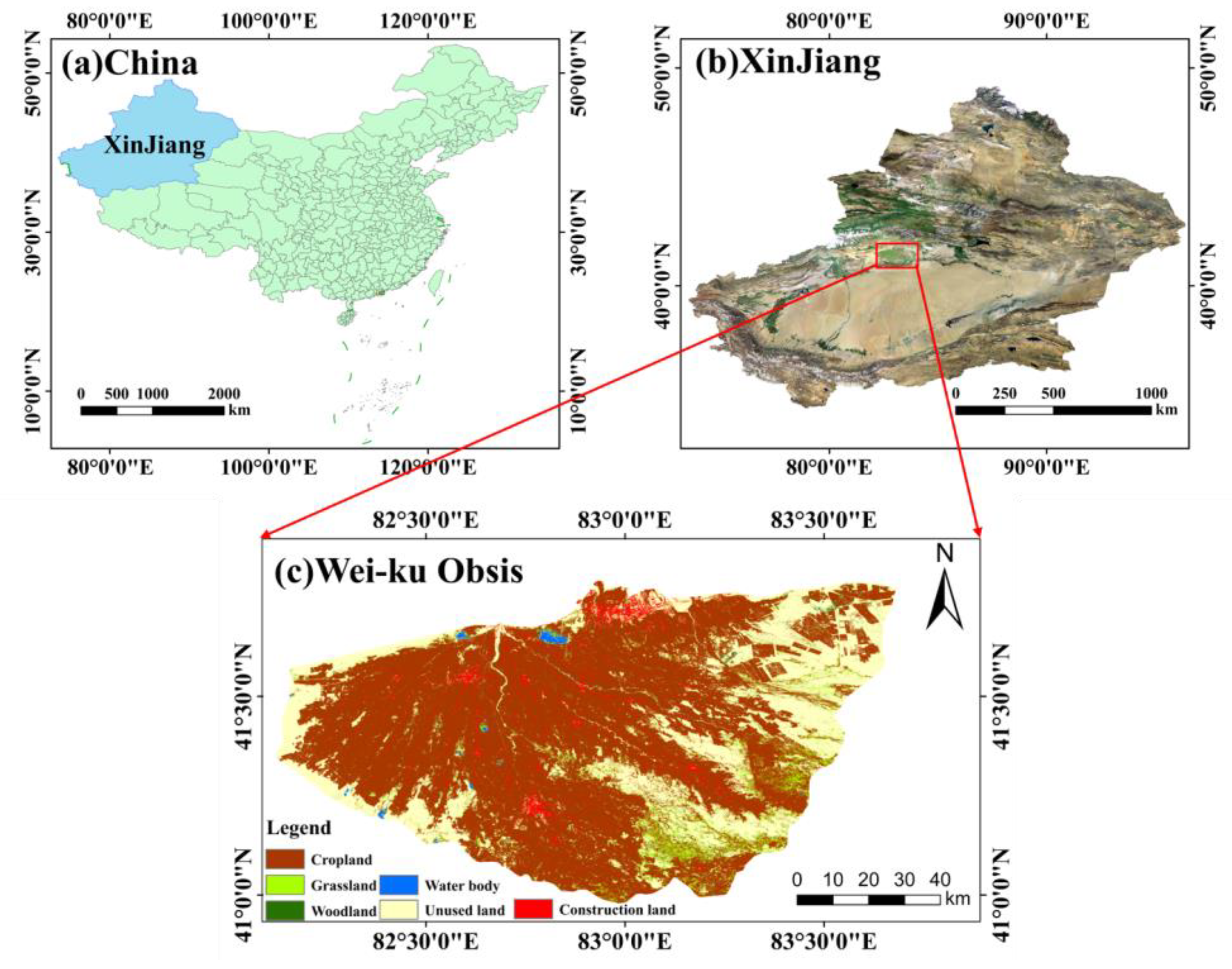
Figure 1. Overview of the study area. (a) Location of the study region within the map of China; (b) location within Xinjiang; (c) land use types within the study area.
Remotesensing 17 02737 g001
Figure 2. Schematic of sampling points at different depths and years.
Remotesensing 17 02737 g002
Figure 3. Scatter plots of different models at various soil depths.
Remotesensing 17 02737 g003
Figure 4. Spatial distribution of soil moisture at different depths in the Wei-Ku Oasis in 2024.
Remotesensing 17 02737 g004
Figure 5. Spatial distribution of surface soil moisture in the Wei-Ku Oasis from 2017 to 2024.
Remotesensing 17 02737 g005
Table 1. Statistics of measured sample points at each soil depth.
Year0−10 cm10–20 cm20–40 cm40–60 cm
Sample303299190173
Table 2. Indices and their formulas.
IndexFormulaReference
Original band B l u e , G r e e n , R e d , N I R , S W I R 1 , S W I R 2 [35]
Normalized differential vegetation index (NDVI) ( N I R R e d ) / ( N I R + R e d ) [36]
Kernel Normalized Difference Vegetation Index (KNDVI) K x n i r , x n i r K x r e d , x r e d K x n i r , x n i r + K x r e d , x r e d [37]
Enhanced vegetation index (EVI) 2.5 [ ( N I R R ) / ( N I R + 6 × R 7.5 × R + 1 ) ] [38]
Fusion vegetation index (FVI) 2 ρ N I R ρ R e d   ρ S w i r 1 2 ρ N I R + ρ R e d + ρ S w i r 1 [39]
Green Leaf Index (GLI) 2 × G r e e n R e d B l u e 2 × G r e e n + R e d + B l u e [40]
Global Vegetation Moisture Index (GVMI) N I R + 0.1 ( S W I R 1 + 0.02 ) N I R + 0.1 + ( S W I R 1 + 0.02 ) [41]
Combined Spectral Response Index (COSRI) ( B l u e + G r e e n N I R + R e d ) ( N I R R e d N I R + R e d ) [41]
Atmospherically Resistant Vegetation Index (ARVI) N I R ( 2 × R e d B l u e ) N I R + ( 2 × R e d B l u e ) [42]
Soil-Adjusted Vegetation Index (SAVI) 1 + L N I R R e d N I R + R e d + L , L = 0.5 [43]
Modified Soil-Adjusted Vegetation Index (MSAVI) [ 2 N I R + 1 ( 2 N I R + 1 2 8 ( N I R R ) ) 0.5 ] / 2 [42]
Optimized Soil-Adjusted Vegetation Index (OSAVI) 1.16 ( N I R R e d ) ( N I R + R e d + 0.16 ) [44]
Modified Simple Ratio (MSR) ( N I R R 1 ) / N I R R + 1 1 2 [45]
Near-Infrared Reflectance of Vegetation (NIRv) N D V I × N I R [46]
Near-Infrared Normalized Index (NNIR) N I R N I R + R e d + G r e e n [47]
Red Nommalized Index (NR) R e d ( N I R + R e d + G r e e n ) [48]
Difference Vegetation Index (DVI) N I R R e d [42]
Renormalized Difference Vegetation Index (RDVI) N I R R e d N I R + R e d [45]
Ratio vegetation index (RVI) N I R / R e d [49]
Infrared position vegetation index (IPVI) N I R ( N I R + R e d ) [50]
Visible and shortwave infrared drought index (VSDI1) 1 [ S W I R 1 B l u e + ( R e d B l u e ) ] [51]
Visible and shortwave infrared drought index (VSDI2) 1 [ S W I R 2 B l u e + ( R e d B l u e ) ] [51]
Temperature Vegetation Dryness Index (TVDI) T s T s , m i n T s , m a x   T s , m i n [52]
Normalized Multi-band Drought Index (NMDI) N I R ( S W I R 1 S W I R 2 ) N I R + ( S W I R 1 S W I R 2 ) [48]
Normalized Difference Water Index (NDWI) ( G r e e n N I R ) / ( G r e e n + N I R ) [53]
Normalized Difference Moisture Index (NDMI) ( N I R S W I R ) / ( N I R + S W I R ) [54]
Modified Normalized Difference Water Index (MNDWI) ( L S T L S T m i n ) /   ( L S T m a x   L S T m i n ) [53]
Vegetation water supply index (VSWI) N D V I / L S T [55]
Normalized Difference Built-up Index (NDBI) S W I R N I R S W I R + N I R [54]
Normalized Difference Bareness Index (NDBSI) S W I R + R e d N I R S W I R + R e d + N I R [56]
Tasseled Cap Brightness (TCB) 0.3029 B l u e + 0.2786 G r e e n + 0.4733 R e d + 0.5599 N I R + 0.508 S W I R 1 + 0.1872 S W I R 2 [57]
Tasseled Cap Greenness (TCG) 0.2941 B l u e 0.243 G r e e n 0.5424 R e d + 0.7276 N I R + 0.0713 S W I R 1 0.1608 S W I R 2 [57]
Tasseled Cap Wetness (TCW) 0.1511 B l u e + 0.1973 G r e e n + 0.3283 R e d + 0.3407 N I R 0.7117 S W I R 1 0.4559 S W I R 2 [57]
Land Surface Temperature (LST) [52]
Vertical transmit and vertical receive (VV) [58]
Vertical transmit and horizontal receive (VH) [58]
SUM_VVVH V V + V H [58]
R_VHVV V H / V V [58]
ND_VVVH ( V V V H ) / ( V V + V H ) [58]
D_VVVH V V V H [58]
SR_VHVV ( V H / V V ) 2 [58]
Table 3. Descriptive statistics of soil moisture at different depths.
Soil
Properties
Minimum (%)Maximum (%)Mean (%)Median (%)Standard Deviation (%)Coefficient of Variation (%)Skewness
0–10 cm0.4330.4710.6010.486.3960.290.23
10–20 cm1.2328.4314.3114.535.4738.23−0.13
20–40 cm0.8137.9114.7614.376.6444.960.23
40–60 cm1.1834.8015.7815.547.1445.250.15
Table 4. Statistics of optimal variable combinations selected by the BOSS algorithm.
Deep/cmNumber of FeaturesOptimal Feature Combination
0–106Green, FVI, GVMI, NDMI, NDVI, SUM_VVVH
10–209Blue, SWIR2, COSRI, NNIR, RDVI, SAVI, SUM_VVVH, TCW, VSDI2
20–408LST, NDBI, NDMI, NDVI, SAVI, SUM_VVVH, VH, VV
40–606SWIR2, GVMI, MSR, TCB, TCW, VV
Table 5. Parameter settings for each model.
Network typeLayersKernel SizeHidden_Size (L)Activation Functions
CNNConvolutional3 ReLU
Convolutional3 ReLU
Pooling2
Fully connected 1ReLU
LSTMLSTM 64Sigmoid, Tanh
Fully connected 1ReLU
CNN-LSTMConvolutional3 ReLU
Convolutional3 ReLU
Pooling2
LSTM 50Sigmoid, Tanh
Fully connected 1ReLU
Table 6. Inversion accuracy of different models at various soil depths.
Deep/cmModelTrainTest
R2MAE (%)RMSE (%)R2MAE (%)RMSE (%)
0–10 cmCNN0.593.474.260.543.043.82
LSTM0.523.784.610.493.254.02
CNN-LSTM0.653.023.970.642.753.39
10–20 cmCNN0.503.294.130.452.663.26
LSTM0.493.494.280.472.272.87
CNN-LSTM0.623.053.660.592.142.66
20–40 cmCNN0.583.744.740.522.573.14
LSTM0.523.845.140.452.493.06
CNN-LSTM0.593.294.430.542.703.27
40–60 cmCNN0.554.165.190.522.973.69
LSTM0.514.465.560.462.833.31
CNN-LSTM0.593.844.890.593.063.80
Disclaimer/Publisher’s Note: The statements, opinions and data contained in all publications are solely those of the individual author(s) and contributor(s) and not of MDPI and/or the editor(s). MDPI and/or the editor(s) disclaim responsibility for any injury to people or property resulting from any ideas, methods, instructions or products referred to in the content.