Article

Standard Classes for Urban Topographic Mapping with ALS: Classification Scheme and a First Implementation

1
Institute of Geodesy and Geoinformatics, Wrocław University of Environmental and Life Sciences, 50-375 Wrocław, Poland
2
Department of Geodesy and Geoinformation, Technische Universität Wien, 1040 Vienna, Austria
*
Author to whom correspondence should be addressed.
Remote Sens. 2025, 17(15), 2731; https://doi.org/10.3390/rs17152731
Submission received: 22 May 2025 / Revised: 7 July 2025 / Accepted: 28 July 2025 / Published: 7 August 2025

Abstract

Research regarding airborne laser scanning (ALS) point cloud semantic segmentation typically revolves around supervised machine learning, which requires time-consuming generation of training data. Therefore, the models are usually trained using one of the benchmarking datasets that cover a small area. Recently, many European countries published classified ALS data, which can be potentially used for training models. However, a review of the classification schemes of these datasets revealed that these schemes vary substantially, therefore limiting their applicability. Thus, our goal was three-fold. First, to develop a common classification scheme that can be applied for the semantic segmentation of various ALS datasets. Second, to unify the classification scheme of existing ALS datasets. Third, to employ them for the training of a classifier that will be able to classify data from different sources and will not require additional training. We propose a classification scheme of four classes: ground and water, vegetation, buildings and bridges, and ‘other’. The developed classifier is trained jointly using ALS data from Austria, Switzerland, and Poland. A test on unseen datasets demonstrates that the achieved intersection over union accuracy varies between 90.0–97.3% for ground and water, 68.0–95.9% for vegetation, 77.6–94.8% for buildings and bridges, and 13.5–52.7% for ‘other’. As a result, we conclude that the developed method generalizes well to previously unseen data.

1. Introduction

Airborne laser scanning (ALS) point clouds are an important source of information for city-scale facility management and planning, building information retrieval, architectural heritage documentation, and creation of decision support systems. However, they can be used most efficiently when they are classified into a well-designed and meaningful set of semantic classes. Therefore, point cloud semantic segmentation often constitutes the first step in processing ALS data. The information about point cloud classification is used for many urban applications including tree and building modelling (e.g., [1,2]), building reconstruction (e.g., [3]), creating 3D city models (e.g., [4]), roof parametrization for the purpose of solar panel installation (e.g., [5]), building damage monitoring (e.g., [6]), and many others. As a result, its accuracy highly influences the accuracy of the delivered products. At the same time, the amount and complexity of point cloud data make it impossible to manually label all of the points of a large-scale urban scene. Therefore, a reliable and automatic point cloud semantic segmentation is of key importance for many ALS data applications.
While the production-level software usually implements unsupervised methods for point cloud semantic segmentation (e.g., filtering of ground vs. off-terrain [7,8]), nowadays, the attention of the research community is focused on deep learning models, as recent experiments suggest that they outperform traditional algorithms in terms of point cloud semantic segmentation accuracy (e.g., [9]). However, deep learning models require a large amount of training data and their preparation is time consuming, expensive, and needs to be performed for each dataset separately. Since there are still few commonly available and precisely classified ALS datasets [10], data availability constitutes one of the main limitations for the development of deep learning methods. Because of this reason, most of the models are trained and validated on one of a few available benchmarking datasets (e.g., [11,12]). However, while the benchmarking datasets are characterized by high classification accuracy, their spatial extent is usually very limited, which may affect the reliability of the estimation of classification accuracy.
Recently, many European countries decided to publish their national (and city-wise) ALS datasets. Most of them include information about the classification of each point. Usually, the classification is provided by an automatic algorithm and therefore its quality is not comparable to benchmarking datasets. However, several countries decided to provide high accuracy, sometimes manually corrected classification for their national point clouds (e.g., Switzerland). Although the classification accuracy of these datasets is probably lower than benchmarking data, the spatial extent of the point cloud is very large, thus enabling extensive training and testing of deep learning networks. As a result, recently, more and more of these datasets have been used for the training and testing of point cloud semantic segmentation models (e.g., [13,14,15,16]).
Usually, both when benchmarking and national data are used, each deep learning model is trained and tested on data from the same dataset (e.g., [9,12,16]). Thus, in most cases, the comprehensive scalability (here, we mean the possibility of successfully applying the classifier to many other datasets than it was trained on, also referred to as generalizability) of deep learning remains unexplored. However, there are some publications that, to some extent, address the problem of the scalability of deep learning models (e.g., [11,17,18]). However, in the case of these papers, the testing of the generalizability of the model was restricted to only one benchmarking dataset and the possibility of joining the datasets in the training phase was not investigated. This idea was pursued by [19], who proposed to create a dataset that consists of four available ALS datasets of high classification accuracy for training and evaluating the performance of ground filtering models (both traditional and deep learning-based). However, in [19], the scalability of deep learning models is evaluated using only one dataset. Moreover, in contrast to our work, the investigations in this paper are focused on point cloud filtration tasks (or binary semantic segmentation) instead of multi-class semantic segmentation. This, in turn, enables the authors to avoid the problem related to different classification schemes between the datasets.
Therefore, in this paper, we present the results of the investigations of the scalability of deep learning models to the previously unseen ALS data. Our aim was to investigate if a classifier can generalize into recognizing objects based on their features regardless of the differences in the data. For this purpose, we trained a deep learning model jointly using national ALS datasets of urban areas in Austria, Poland, and Switzerland that represented one city in each of the countries. We decided to employ national datasets as they represent a larger spatial extent than benchmarking datasets. As a result, the variability of objects present in the training data is larger. Joining several datasets for the training stage helped us to prevent the network from learning the characteristics of 3D points which are typical for a specific class and specific laser scanning dataset, rather than the characteristics of a specific class in relation to other classes. Moreover, training with data of different characteristics (e.g., point density, acquisition season, equipment used, etc.) should improve the scalability of the classifier.
To reliably measure the extent of the scalability of the developed classifier, we reviewed the available benchmarking and national datasets and used them to extensively test the accuracy of the model. However, using national datasets poses an additional challenge as different national datasets reflect class definitions, which are adapted to the different national requirements. Different concepts of representing topographic objects can partly be solved by ontology alignment, which aims at matching semantically equivalent objects that are described differently in two or more ontologies (e.g., [20]). Our aim is, however, the unification of concepts.
Here, we provide a review of the differences between classification schemes available in various countries. As a result, we recommend a set of classes that allows for using ALS data from multiple countries, represents the most common land cover objects in the cities, and generalizes well to various ALS datasets. The proposed classes are ground and water, buildings and bridges, vegetation, and ‘other’. The introduction of a general classification scheme for all ALS data produced in Europe would have a huge potential in terms of further applications. It would allow for an easy comparison of the data, facilitate the application of point cloud processing methods for the whole continent, and ensure the comparability and coherence of the conclusions drawn from the point cloud analysis. Thus, we do not target ontology alignment, but a homogenous definition independent of national custom solutions. The proposed classes aimed at simplicity and, as a result, present the smallest meaningful number of classes that are suitable for various point cloud processing applications. Therefore, the proposed classification scheme does not limit the national mapping agencies in providing a more detailed set of classes that can be easily generalized to the proposed set of four classes.
The first step for the standardization of point cloud classification schemes was performed by the introduction of the LAS standard [21]. However, during the creation of this standard, the creators aimed at including all of the classes used by different entities (companies, authorities, etc.). Because of that, the number of classes that can be defined in a las file is very large and, as a result, the entities have to choose which classes are important for their applications. This, in turn, leads to large differences between classification schemes among different countries. In contrast to this approach, we suggested a small number of classes that are universal for various applications. We do not divide any classes that are defined in the LAS standard but rather merge them to obtain the more general and most important set of classes. Moreover, as a result of the performed investigations, we provide the readers with both a well-tested estimation of the scalability of the created deep learning model and a trained universal classifier that allows for an accurate semantic segmentation of the high variability of different datasets. Using this classifier enables us to avoid expensive and time-consuming preparation of training data for every classification task separately. Apart from it being useful for a variety of new point cloud processing tasks, it may help to improve the accuracy of some of the existing national datasets. Moreover, it might provide the opportunity to unify the classification of some of the datasets into the four proposed classes. Having a trained classifier together with a thorough evaluation of its generalization capabilities might also help the acceleration of this process. While these additional possibilities motivate our work, we did not specifically test them.
The first results of the investigations were published in [22]. Here, we present an extended investigation that includes a classifier trained using more training data, a more extensive evaluation of the results that includes a large amount of previously unseen data, and an in-depth review of the classification schemes and analysis of differences of characteristics for each dataset. The novelty of the investigations lies in providing an overview of available data, the analysis of their usability for the training of deep learning models, the methodology of data selection, and the proposition of a classification scheme and approach for the training of classifiers using multiple available national urban data datasets, rather than in advancing models for deep learning.

1.1. Related Work

1.1.1. Deep Learning-Based Point Cloud Semantic Segmentation Methods

Recently, many deep learning techniques were developed for the semantic segmentation of point clouds. These techniques can be divided into two main groups: structure grid-based and point cloud-based methods (e.g., [23]).
The structure grid-based methods aim at transforming the point cloud into a regularly structured object. These methods can be further divided into projection-based, voxel-based, and other. Most of the projection methods represent point clouds as a set of images that are generated from different angles and locations. Then, the point cloud is processed using standard convolutional neural networks that are used for image processing. This approach was first introduced by [24] for the point cloud classification tasks. The high accuracy of the developed network on the ModelNet dataset led to the investigations of the possibility of applying these methods for a semantic segmentation task. For instance, Ref. [25] proposed a SnapNet network that makes snapshots of the point cloud, uses the convolutional neural network to label each image, and then connects the labels to 3D points. Although projection-based methods allowed for the achievement of high accuracies for classification and semantic segmentation tasks, their accuracy is highly influenced by the angle of the projection. Moreover, the projection of the point clouds leads to the loss of spatial information [26]. The voxel-based approaches transform an unstructured point cloud into a regular voxel grid. Then, a 3D convolution is performed to label each voxel, and the labels are extrapolated to the point cloud. An example of the realization of this approach is a VoxNet [27] neural network that was designed for point cloud classification tasks. However, voxel-based approaches waste a lot of computation capabilities by calculating convolutions over empty voxels. As a result, due to the high computational and memory usage, these methods could not be directly applied to large-scale investigations. To optimize the procedure, Ref. [28] proposed to take the advantage of the sparsity of the point cloud by restricting the convolution operation to the non-empty voxels only. As a result, the data dilation problem can be minimized. The other group of structure grid methods consists of networks that use higher dimensional lattices. For instance, the SplatNet [29] network uses a bilateral convolutional layer to convert points into a 6D lattice which is then used to calculate the convolutions. The SFCNN [30] neural network projects points onto an icosahedral lattice and its fractals.
Despite the relatively good accuracies achieved by voxel- and projection-based methods, most commonly used methods for point cloud semantic segmentation belong to the group of point-based approaches. The first network architecture that enabled the processing of raw point cloud data was PointNet [31]. The proposed architecture learns features by utilizing multilayer perceptron (MLP) layers. Although PointNet achieved state-of-the-art performance on numerous datasets, it does not capture local dependency between the points. This causes limitations connected with fine-grained local patterns [29]. To solve this problem, several solutions were developed that employ hierarchical architectures in order to accumulate neighborhood information. For instance, Ref. [32] proposed a PointNet++ architecture that is able to derive geometric features in different scales by first learning the local features and then increasing the scale using the nearest neighbor approach. Another example of an MLP-based network is RandLA-Net [33], which employs random sampling for an efficient processing of large-scale scenes. In this network, the features are extended with relative positions of neighboring points. Then the attentive pooling operation is performed to select relevant features and geometric patterns of the point cloud. The preservation of geometric features is also supported by progressively expanding the receptive field. A different approach for point-based semantic segmentation is based on convolution operators that are adjusted to the processing of 3D point clouds. Many of these approaches treat weights of convolution operations as a continuous function of the point coordinates and then approximate this function using an MLP. For example, this approach was used in PointCNN [34], which uses X-transformation for a simultaneous weighting and permuting of input features. Permutation invariance was achieved by the PointConv network [35], which uses an MLP to approximate weights of the convolution operation and applies an inverse density scale to the learned weights to address the non-uniform sampling of the point cloud. In the alternative approach, the convolution kernel is explicitly defined. For instance, in Flex-convolution [36], linear functions are used for modelling the kernel. Ref. [37] models the kernel using a set of polynomial functions with weights associated with each neighbor. Some studies propose to use a subset of points to define the area of the application of kernel weights. For instance, KPConv [38] utilized radius neighborhoods and proposed a deformable kernel where both the weights and kernel point positions are learned. As a result, the network is more robust to different point densities. Another group of point-based deep learning models employs graph structures by treating every point as a node. For instance, Ref. [39] proposed a Dynamic Graph Convolution (DGCNN) neural network that constructs the graph based on the local neighborhood. Then, it applies edgeConv layers to calculate features. The DGCNN architecture differs from standard graph methods as edges of the graph are updated after each edgeConv layer.
The detailed overview of the existing deep learning models and their applications can be found in [23,26,40,41,42,43].

1.1.2. Semantic Segmentation of ALS Data

Most methods described in Section 1.1.1 were developed for the semantic segmentation of synthetic or indoor benchmarking datasets. Some of them were also tested using outdoor static laser scanning data. However, recently, many of them were successfully applied for processing large-scale airborne laser scanning datasets. Moreover, many new methods were developed directly for the processing of outdoor scenes.
Usually, the methods are trained and validated using available benchmarking datasets. For instance, Ref. [18] investigated the generalization possibilities of the KPConv neural network for the semantic segmentation of Vaihingen and LASDU benchmarking datasets. To unify the classes in both datasets, the Vaihingen dataset was reclassified into five classes. Ref. [12] proposed a modification of the PointNet architecture that utilizes a 1D fully convolutional network for processing terrain-normalized points and spectral data together. Ref. [44] proposed to modify the PointNet++ architecture to enhance the capabilities of the network to extract local and global features. Then, the method was tested using the Vaihingen dataset and the generalization ability of the method was evaluated on the GLM(B) dataset. Ref. [45] proposed to use the point transformer method together with the rule injection strategy to classify Vaihingen, Hessigheim, and S3DIS benchmarking datasets. The rule injection strategy realizes the Knowledge Enhanced Neural Network concept and enables the inclusion of different types of logic rules in the stage of network training. Ref. [46] proposed a receptive field fusion-and-stratification network (RFFS-Net) that allows for the exploitation of the information from various sizes of the receptive field. The network was evaluated using Vaihingen, LASDU, and 2019 IEEE-GRSS Data Fusion Contest (DFC) benchmarking datasets. Ref. [11] constructed a dense hierarchical architecture (GADH-Net). The architecture is based on geometry-aware convolution that aims at learning high-level features based on handcrafted features. The results were evaluated using the Vaihingen benchmarking dataset and the generalization ability of the network was evaluated using the 2019 IEEE GRSS Data Fusion Contest 3D dataset.
Due to the limited accessibility of large amounts of accurately labelled ALS datasets, recently more and more investigations employ other national or city-wise datasets, often along with benchmarking datasets, in order to train and validate deep learning models. The most commonly used dataset is AHN (Actueel Hoogtebestand Nederland). For instance, Ref. [47] proposed a modified PointNet++ architecture together with a data augmentation strategy that enables the utilization of the deep features generated for multi-scale point sets. The performance of the network was evaluated based on Vaihingen and part of the AHN dataset. The AHN point cloud covered 4 km2 of the Rotterdam city center and was classified into five classes. Ref. [48] applied submanifold sparse convolutional networks (SparseCNN) to classify the Vaihingen dataset and the AHN 3 dataset. The AHN 3 dataset covered 4 km2 of the residential area of Deventer. The semantic segmentation was performed using five classes. Ref. [15] applied the PointNet network to classify AHN 2 and AHN 3 datasets and to investigate the possibility of the generalization of the classifier between those acquisitions. The data included two tiles located in the surroundings of Utrecht and Delft covering 31.25 km2 each. Ref. [16] proposed to use DGCNN architecture in order to classify AHN 3 and Surabaya (Indonesia) areas covering 125 km2 and 5 km2, respectively. However, for the Surabaya area, the reference labels had to first be generated before training. For both regions, the point cloud was classified into four classes but the set of classes was different in each of the datasets. Ref. [14] projected the point cloud into a horizontal plane and proposed a multi-scale fully convolutional network architecture to perform 2D image semantic segmentation. The method was evaluated using the ISPRS Filter Test Dataset for a filtration task and 22 samples of the AHN 3 dataset with a size of 0.25 km2 for multi-class semantic segmentation and filtration. The point cloud filtration task was also investigated by [49], who evaluated three approaches for ground classification. The approaches included a heuristic method, PointNet network, and deep convolutional network based on SegNet that requires the projection of the point cloud into a plane. The results were evaluated using the AHN 3 dataset and Vaihingen datasets. Ref. [13] proposed a point cloud filtration method that uses handcrafted features as an input to a deep learning fully connected deep neural network. The accuracy of the method was evaluated using AHN 3 data and ACT (Luxembourg) data covering 31.25 km2 and 0.5 km2, respectively. All of these investigations employ different parts of the AHN 3 and AHN 2 point clouds. However, other datasets are also used for deep learning investigations. For instance, Ref. [50] proposed to use the Atrous XCRF method together with PointCNN deep learning architecture in order to minimize overfitting by introducing noise in the training procedure. The results were evaluated based on the Vaihingen dataset and the generalization capabilities were investigated using the Bergen dataset (Norway). The use of handcrafted features was proposed by [51], who included them in PointNet and PointNet++ architectures to classify the ALS and mobile laser scanning dataset of Tainan into four classes. The filtration task was investigated by [19] using four deep learning architectures: PointNet++, KPConv, RandLA-Net, and SCF-Net. The models were trained and evaluated using a custom dataset that consisted of four datasets from Europe, New Zealand, and North America that covers 47 km2 using overall accuracy and a class-wise IoU metric. The generalization capability of the model was also evaluated on the ISPRS Filter Test Dataset. Ref. [52] proposed adapting PointNet++ for the semantic segmentation of Vaihingen and Vorarlberg (Austria) datasets. The Vorarlberg dataset covers an area of 62.5 km2. However, for this dataset, the labels had to be first automatically generated by commercial software and included six classes. Ref. [9] compared the accuracy of three different deep learning models, SparseCNN, KPConv, and PointNet++, for the semantic segmentation of the dataset of Vienna and a dataset representing powerlines. The dataset of Vienna covered 11.65 km2.
In this paper, we propose to utilize national ALS datasets of three countries (Poland, Austria, and Switzerland) to jointly train a classifier. Then, we test the influence of these datasets on the performance of the classifier and thoroughly investigate the generalization capabilities of the developed classifier using multiple national and benchmarking datasets. The concept of the classifier training using multiple datasets is similar to [19]. However, we investigate the multi-class semantic segmentation problem and provide an extended evaluation of the generalization capabilities of the model. We also address the problem of the variability of classification schemes in the ALS datasets in Europe. Moreover, we propose an approach to the unification of the classification of available datasets together with standard classes that can be used for the generalizable classification of ALS data. For the purpose of these investigations, we selected the SparseCNN neural network [28], which proved to be accurate and effective for the processing of both benchmarking [28,48] and national laser scanning datasets, including ALS data [9].

2. Materials and Methods

2.1. Data

In order to develop a classifier that will be as universal as possible while preserving high classification accuracy, the available European datasets were reviewed. Special attention was put into the identification of datasets that are characterized by high accuracy in classification. This is usually provided by a manual verification processing step that follows the automatic classification. However, since the manual correction of classification is expensive and time consuming, only five appropriate datasets were identified. These datasets were acquired either by mapping agencies or independently by selected cities in five countries: Austria, France, the Netherlands, Poland, and Switzerland.
Since the above national datasets were acquired independently by different countries or cities, they have substantially different characteristics. The differences include, for instance, point density, acquisition time, processing procedure, or classification scheme. Moreover, the datasets were captured by different devices during missions performed according to different flight parameters.
Most of these differences are advantageous because of the purpose of the experiment, as they enable the production of a robust classifier that should be able to process different types of data. However, the differences in classification schemes would lead to high complications in the training procedure. For instance, the same object assigned to different classes in different datasets would confuse the network and lead to lower accuracy in assigning this object to the correct class. Therefore, a universal classification scheme had to be developed in order to exploit as many datasets as possible. To achieve the goal, the differences in classification schemes were described and analyzed.
Moreover, despite the high effort put into manual correction of the classification, every dataset includes some degree of classification errors. This is true for both benchmarking [53] and national [9] datasets. These errors occur with various frequencies in different datasets but are very challenging to measure. However, they influence (to some unknown extent) the ability to train and validate the model, as it is assumed (in both training and validation stages) that the reference data are free of errors. Therefore, when describing each dataset, we provide our observations regarding the classification accuracy collected during the visual inspection of point clouds. Even though this evaluation is qualitative and subjective, it provides insight into the problem and can help explain the results.

2.1.1. Differences in Classification Schemes

The classification schemes were compared for the following datasets collected for selected countries:
(1)
The Netherlands: The newest datasets of the Actueel Hoogtebestand Nederland (AHN) project (AHN3 and AHN4) are analyzed as they contain the classification of the point clouds. Previous editions of the point clouds (AHN1 and AHN2 data collection campaigns) were filtered but not classified. Both analyzed datasets cover the whole country.
(2)
Poland: Two types of datasets are analyzed: the data collected during project “Informatyczny System Osłony Kraju przed nadzwyczajnymi zagrożeniami” (ISOK) and other available data. In the latter case, the data are usually ordered independently by individual territorial division units. However, the data are validated and accepted by the mapping agency. The ISOK data cover the whole country, whereas other datasets are available locally.
(3)
Switzerland: The data are collected and distributed by a mapping agency in the framework of the swissSURFACE3D (©swisstopo) project. The data do not cover the area of the whole country yet but the remaining data are in the collection and processing stage.
(4)
France: The analyzed dataset was collected only for the city of Strasbourg and is not a part of the larger country-wise dataset. This dataset is separate from the French national point cloud mentioned in Table 1.
(5)
Austria: The analyzed data were collected only for the city of Vienna.
The differences between classification schemes for each country are presented in Figure 1. The colors correspond to the ASPRS definition of classes in las files. The same color indicates objects that belong to the same class in a certain dataset. Figure 1 presents only the differences in objects that are present in the point cloud most frequently. More subtle classification differences may also occur in the point clouds, especially in regards to the objects that belong to the ‘other’ class. As a result, it is possible that the accuracy of classification results of the ‘other’ class may be lower than in the case of the rest of the classes.
The analysis of Figure 1 revealed that even for a small subset of available datasets, the differences between the classification schemes are substantial. Some of the differences can be easily unified, for example, vegetation classification in Poland (division into high, medium, and low vegetation) and in Switzerland, France, and Austria (only one vegetation class). This can be fixed by joining all vegetation classes in Polish data or dividing the vegetation class in Austrian, French, and Swiss data (the high, medium, and low vegetation classes are divided solely by height, so no additional processing is needed). However, there are some differences that are very hard to unify, for instance, water classified as ground in Strasbourg or the lack of a vegetation class in the Dutch data (vegetation is included in the other class).
Based on the analysis of the classification differences, the datasets from Poland, Switzerland, and Austria were chosen for the training and testing of the classifier performance, as the classification differences in the case of these datasets are minor.

2.1.2. Selected Training and Testing Datasets

For the datasets from each of the selected countries, one city with surrounding areas was selected for the training of the network and testing its performance during each step of classifier preparation. One city and its surrounding areas should provide enough variation in objects and cover the most common objects that are present in the city. On the other hand, the amount of data should be manageable for the model training. The selected cities are Vienna (Austria), Zurich (Switzerland), and Opole (Poland). The selected cities introduce additional differences between the datasets as they represent cities of very different sizes. As a result, expected architecture types, building densities, and class size ratios should be different in each of the datasets. Moreover, we can expect that larger cities will have a higher variability of building types, whereas smaller cities will be characterized by larger green areas. The basic characteristics of train, test, and validation point clouds are presented in Table 1. While analyzing the differences between the datasets, we focused on the main features that can affect the geometry of the point cloud and its usability for training purposes. These features included the acquisition date, season, point density, classification scheme, and size of the dataset (national-scale, city-scale, and benchmarking). Unfortunately, it was not possible to take into account all of the features that could possibly influence the geometry of the point cloud, such as flying altitude or scanner type as this information is usually not available for the large-scale point clouds.
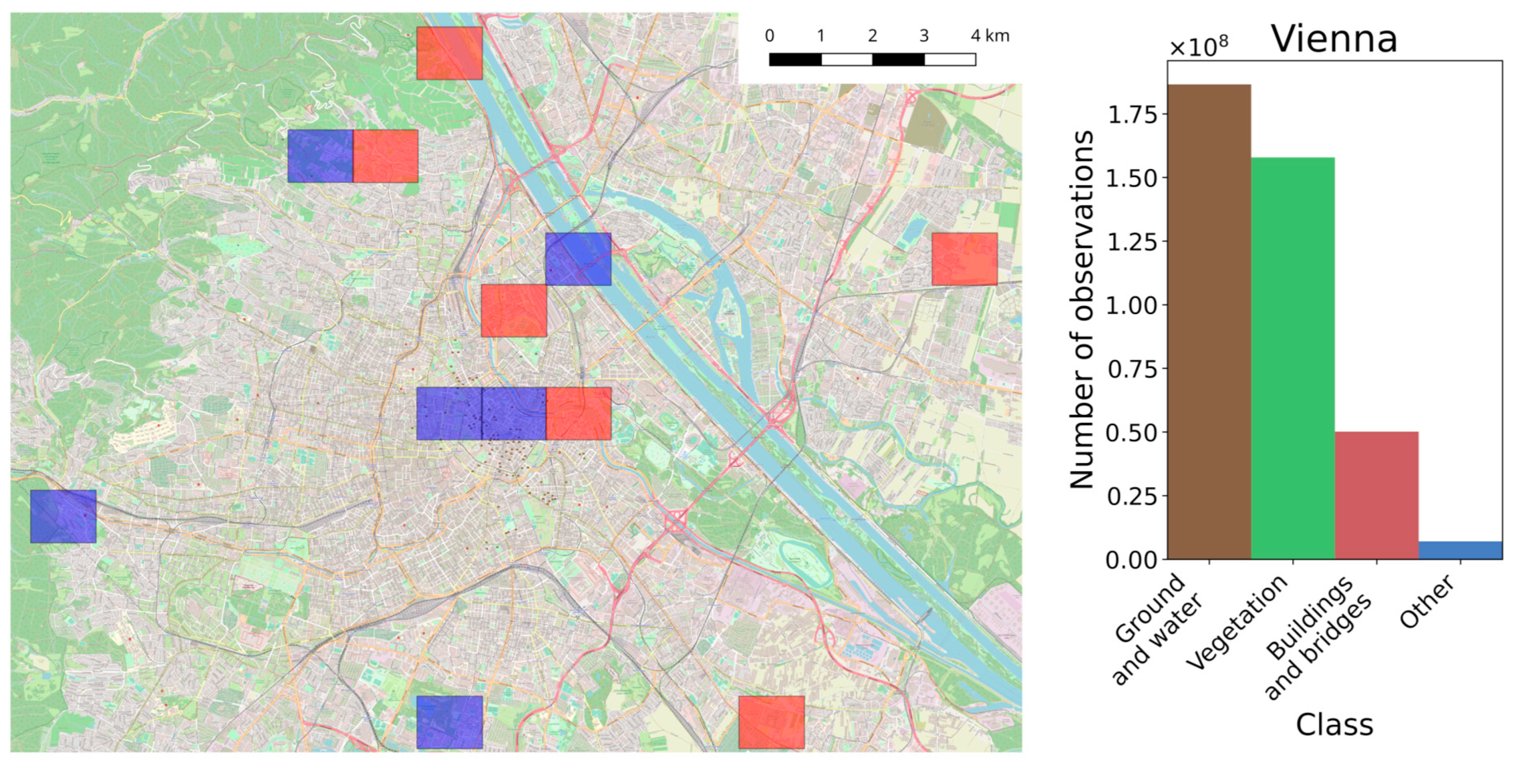
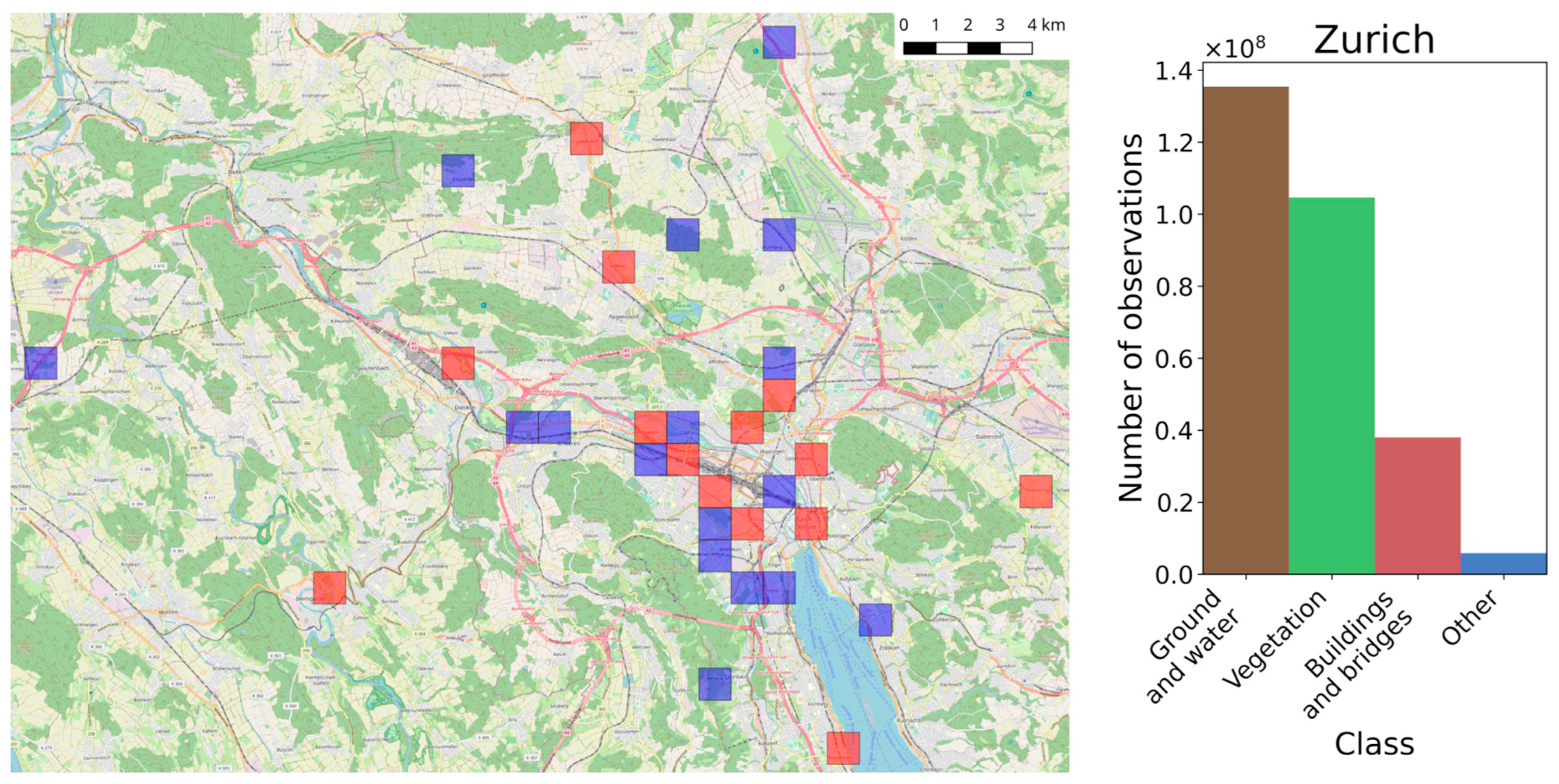
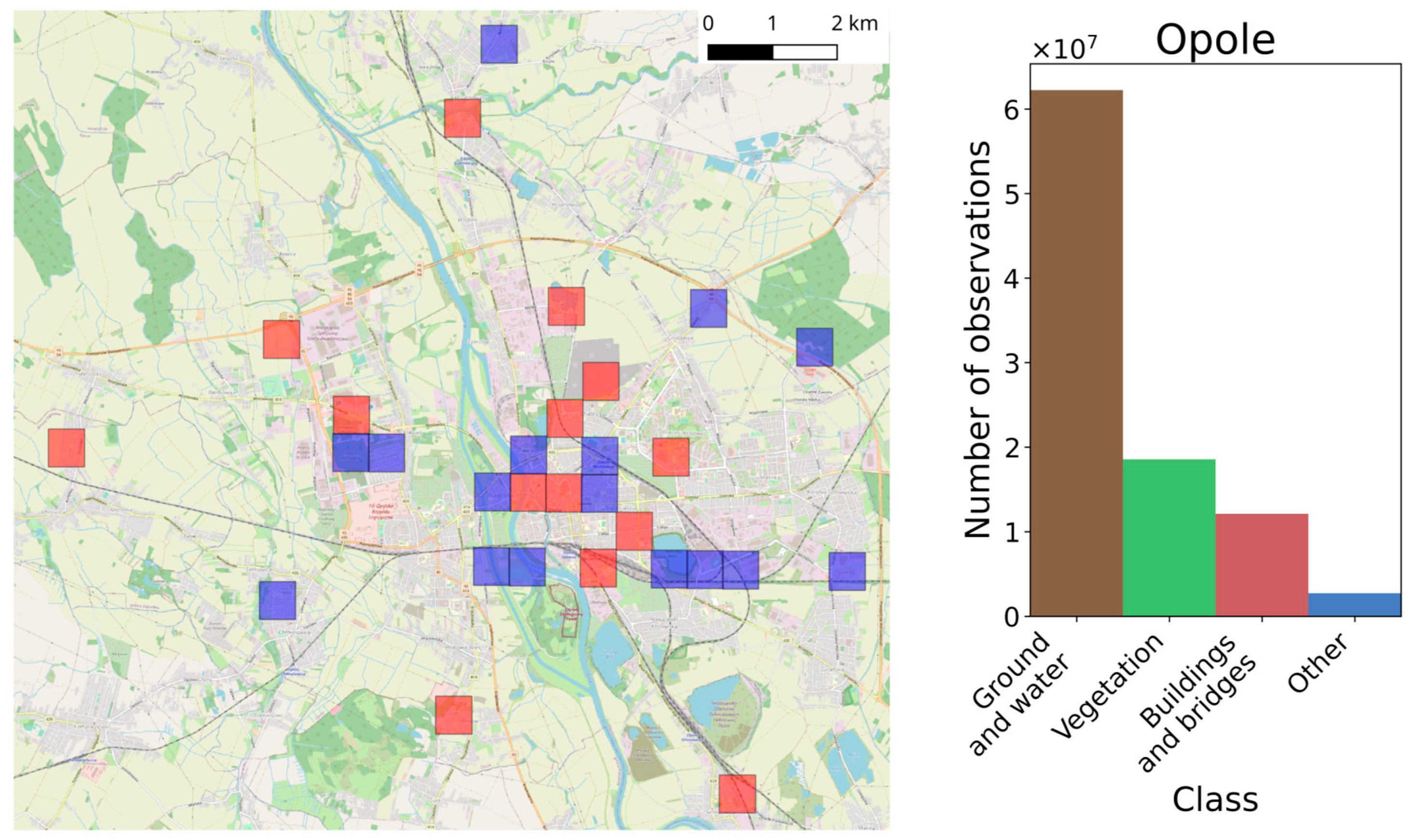
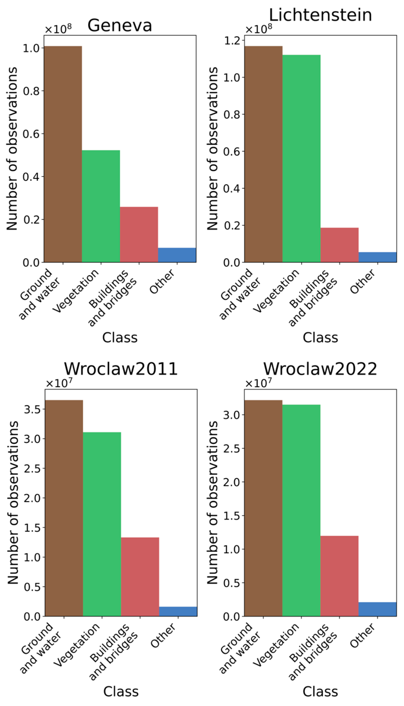
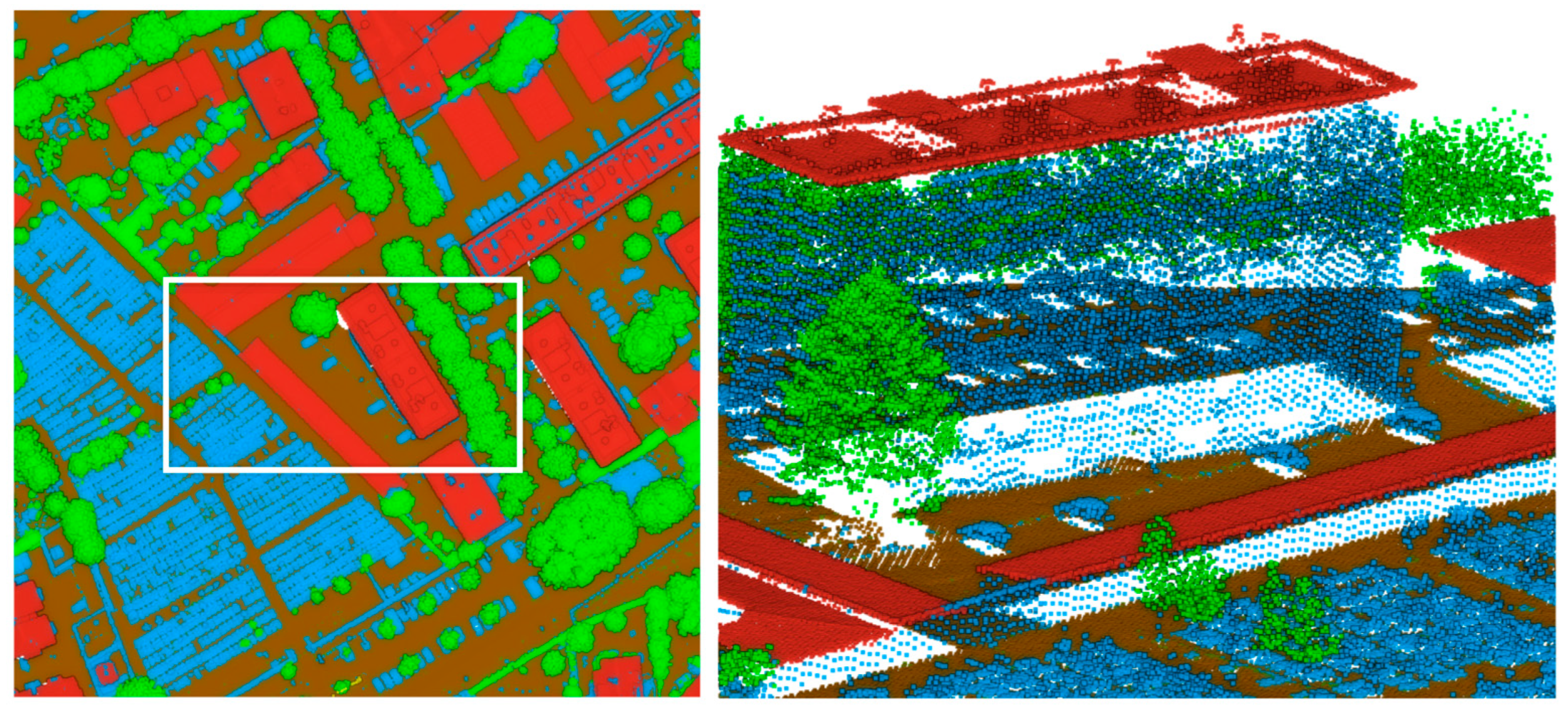
In each city, a set of training and testing tiles was selected. The training and testing tiles were selected in a way so that they represent both the most common objects that are present in the point clouds representing cities as well as more unusual objects. As a result, the following objects are always present in the training tiles: railways, viaducts, rivers, bridges, monuments (if present), different types of buildings (i.e., multi-family, single-family, industrial buildings, shopping centers, and churches), parks, roads (i.e., narrow city roads, highways, etc.), cemeteries, sport facilities, construction sites, etc. In order to make the classifier more robust, tiles were also chosen outside of the cities in the nearby villages and woods. The location of the tiles together with histograms representing class frequencies for each of the datasets are presented in Figure 2, Figure 3 and Figure 4.
The classification accuracy in the selected datasets is generally high and the errors occur relatively seldom. However, the accuracy of the classification of the Opole dataset is lower than for Zurich and Vienna. Thus, errors in this dataset are more common and may influence all of the classes. At the same time, for Zurich and Vienna, the classification errors mostly affect the ‘other’ class and vegetation. In the case of Opole and Zurich, additional tiles covering surrounding areas were also selected as a part of training and validation sets.
For the purposes of training the network, the training dataset was divided into patches that consist of 600 thousand points each, according to the procedure described in [52].

2.1.3. Selected Validation Datasets

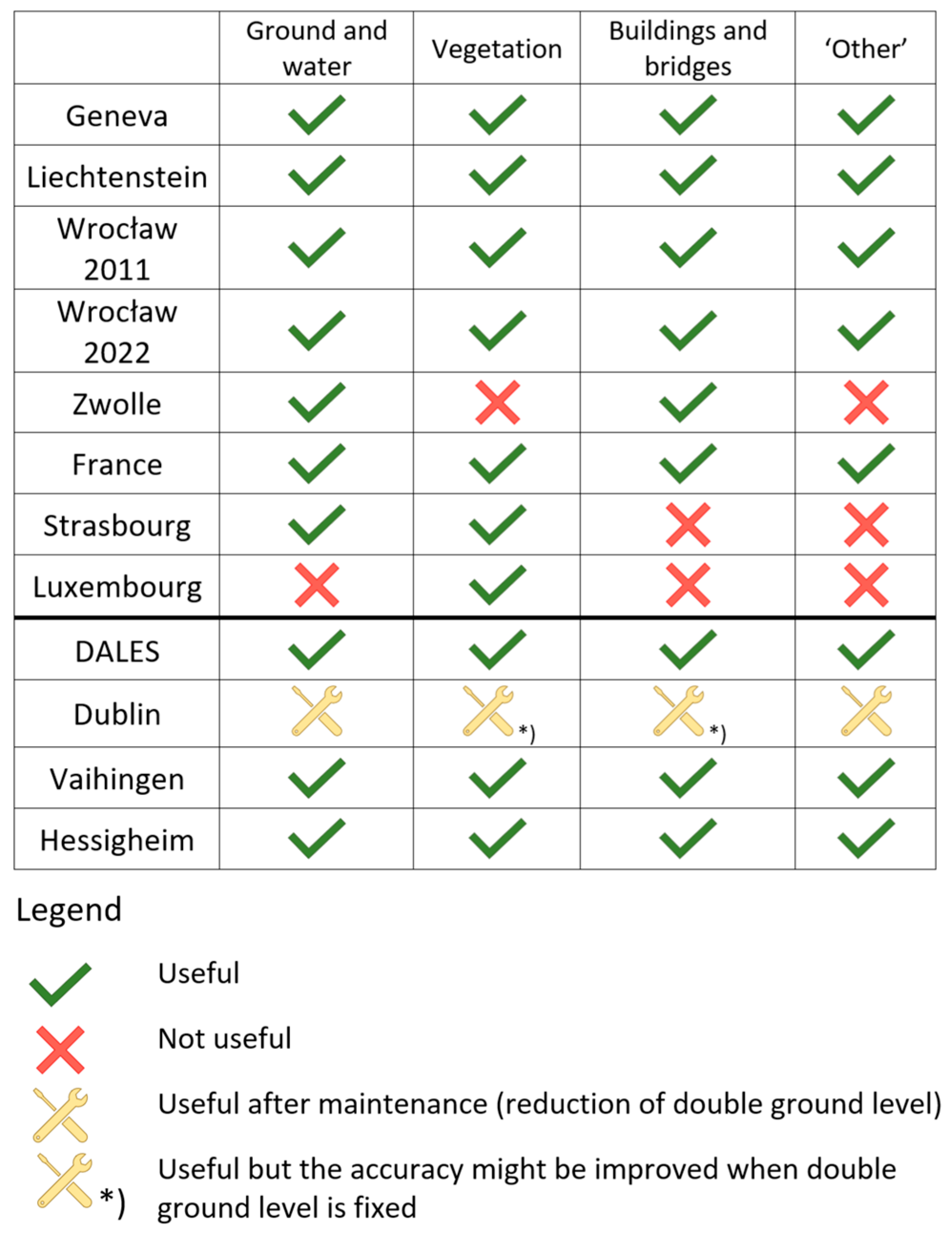
The validation data included selected tiles of ALS point clouds from Geneva, Liechtenstein, Wrocław (acquired in 2011 and 2022), Zwolle, France, Strasbourg, Luxembourg, British Columbia, Vaihingen, Hessigheim, and Dublin. The basic characteristics of these point clouds are presented in Table 1. The usability of these datasets might be restricted to selected classes due to differences in classification schemes and classification errors. The summary of the usability of each dataset is presented in Figure 5.
The validation datasets were divided into following three groups:
(1)
The data collected for Poland and Switzerland but representing different cities than the training data. Additionally, the data from Liechtenstein was included in this group as it was collected jointly with Swiss data.
In the case of Swiss data, the Geneva and Liechtenstein ALS data were selected. The histograms of class occurrences for each dataset are presented in Figure 6. The city of Geneva is located on the other side of the country than Zurich and, as a result, it was collected during different measurement campaigns. On the other hand, Liechtenstein is located rather close to Zurich and the ALS data were collected during the same measurement campaign. However, they are characterized by very different terrain structures, as the city is located in a mountainous area. The classification accuracy of both datasets is very high.
In the case of Polish data, the Wrocław ALS data were selected. However, the measurements were performed during different measurement campaigns (in 2011 and 2022). The data were acquired independently from Opole data and in contrast to any other dataset it represents leaf-on conditions. The classification accuracy of these datasets is lower than in the case of Swiss or Austrian datasets, especially in the case of the 2011 data acquisition period. Thus, selecting a dataset representing the same area, but collected at different times and characterized by different classification accuracies should indicate how much label inaccuracy influences the classification results.
(2)
Data from other European countries, which for various reasons were not suitable for network training. These reasons include substantial differences in classification schemes which were impossible to unify without a potential loss of accuracy, the very small size of the dataset, or a large classification error in one of the classes while obtaining high classification accuracy in other classes.
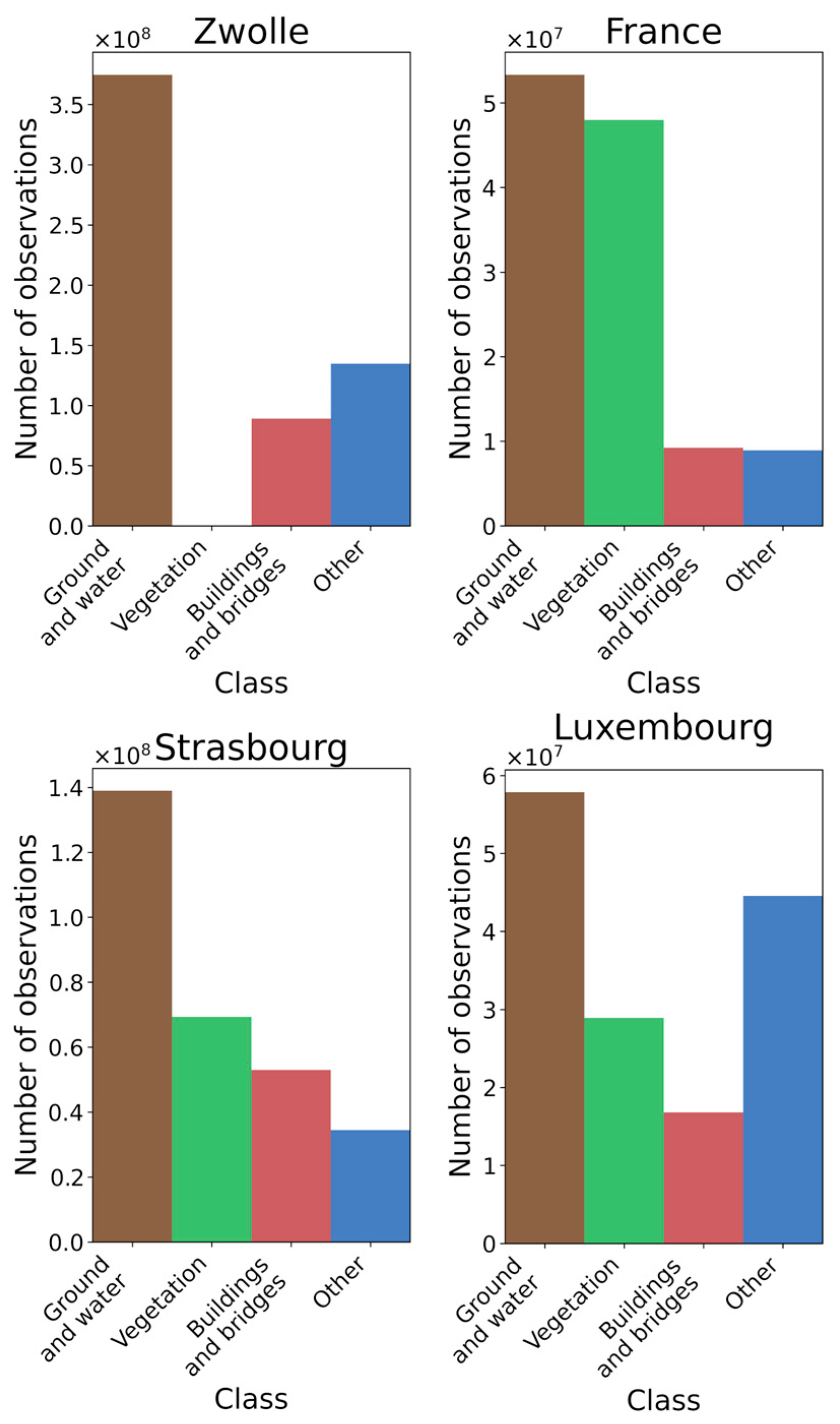
In this group, the data from Zwolle, France, Strasbourg, and Luxembourg were selected. The histogram of class occurrences in each dataset is presented in Figure 7.
The Zwolle dataset is a part of the AHN4 dataset collected for the whole Netherlands. The accuracy of the classification is high and the errors occur very seldom. This dataset could not be used for the training stage because it lacks a vegetation class—the vegetation points are classified into the unclassified (other) class. However, based on this dataset, it is possible to evaluate the accuracy of the ground and water and buildings and bridges classes.
The dataset of France is a part of the French national campaign for collecting ALS data. Currently, the data cover part of the country. In most of the cases, the distributed data are currently not classified. However, there are several tiles available that present the intended classification accuracy. These tiles are very well classified and usually represent complex urban and vegetated areas. The tiles used were selected so that they fit the selection criteria of other testing and training datasets.
The Strasbourg data were published by the city of Strasbourg. The dataset has high classification accuracy. However, it could not be used for the training phase because of facades being included in the ‘other’ class rather than in the building class. However, the accuracy of the vegetation and ground and water classes can be accurately assessed.
The Luxembourg dataset, in general, has relatively good classification accuracy in vegetation and buildings and bridges classes. However, it could not be used for the training of the network because of the large number of ground points being classified as ‘other’ (unclassified). Moreover, the facades of the buildings are included in the ‘other’ class. However, the accuracy of the vegetation class can be accurately evaluated using this data.
(3)
Benchmarking datasets.
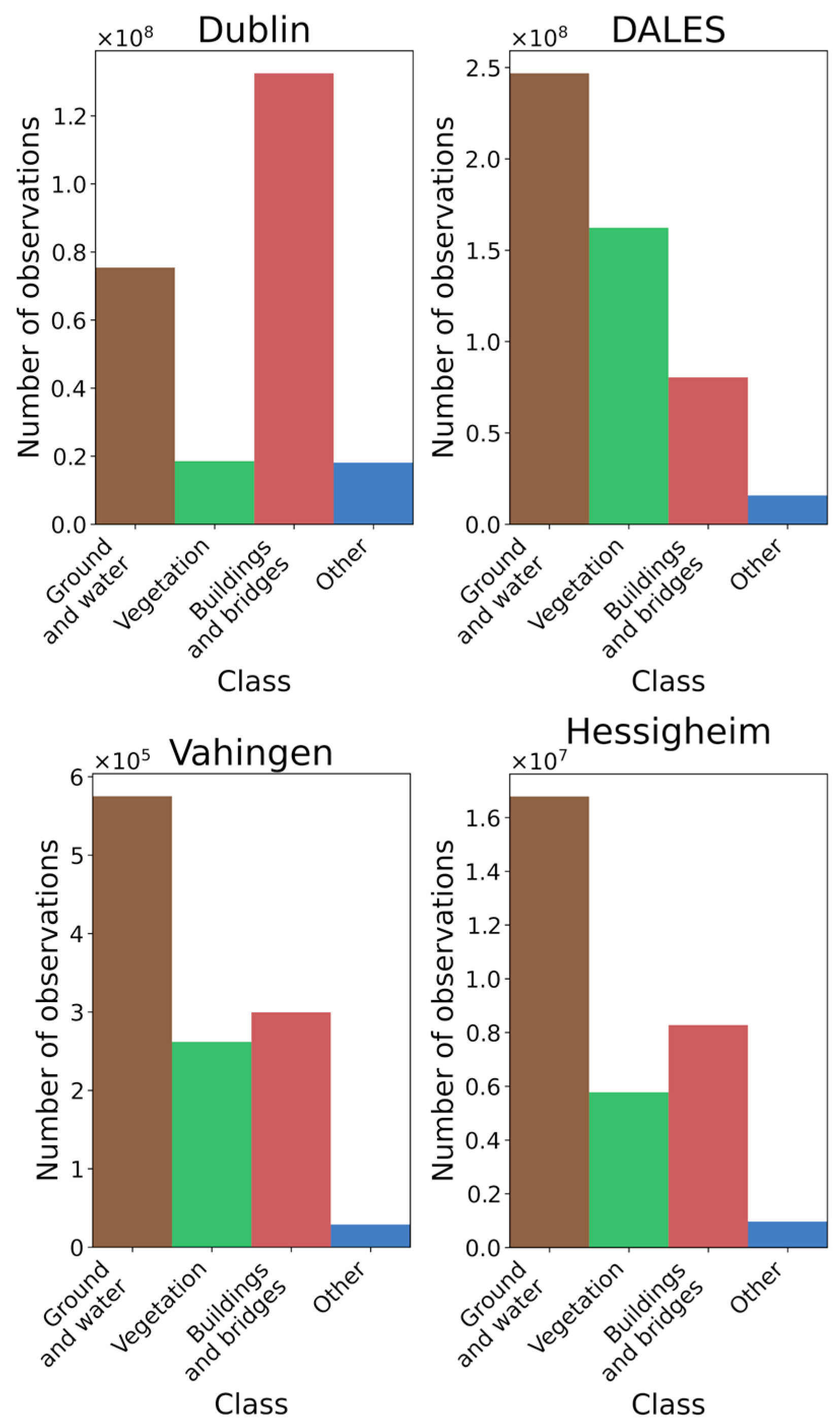
The analysis of the accuracy of the results was also based on four available benchmarking datasets consisting of airborne LiDAR data of Dublin, DALES, Vaihingen, and Hessigheim datasets. The histogram of class occurrences in each of these datasets is presented in Figure 7. The Dublin dataset is an airborne LiDAR point cloud published by the Urban Modelling Group at University College Dublin. The dataset consists of 260 million labelled points that cover an area of 2 km2. More information about the dataset can be found in [54,55]. The DALES dataset was published by the University of Dayton and represents part of the area of British Columbia, Canada [56]. Since the dataset covers a large area, the class distribution is similar to the distribution of classes in country-wise European datasets (Figure 8). The Vaihingen dataset was published by the International Society for Photogrammetry and Remote Sensing and consists of 3 test areas. This dataset has much lower point density than other datasets analyzed in this study. More information about the dataset can be found in [57]. The Hessigheim dataset was published by Institute for Photogrammetry of the University of Stuttgart, ISPRS, and EuroSDR organizations. In this experiment, only the ALS point cloud is used. More information about the dataset can be found in [58]. In the case of benchmarking datasets, some of the classes had to be reassigned to match the set of classes used in this investigation. The details about class reassignment in all datasets can be found in Appendix A.

2.2. Methodology

2.2.1. Classification Scheme

The dataset was classified into four classes: building and bridges, ground and water, vegetation, and other. In order to achieve a robust model, the classification scheme was developed based on the classification of available training data while avoiding, where possible, high class imbalances.
Buildings, bridges, and viaducts were assigned to the same class due to the existing data classification of this type in the Opole dataset. The further automatic processing of this dataset in order to divide the building class into separate classes of buildings and bridges would lead to the creation of additional errors in the training data. The influence of these errors on the accuracy of semantic segmentation would be hard to estimate. Ground and water were merged together due to their high similarity. Since low, medium, and high vegetation classes are distinguished based solely on the point height, the classification was performed into only a general vegetation class. This class can be easily divided into more specific classes in the post-processing stage.

2.2.2. Evaluation Strategy

The model performance was evaluated based on two experiments.
  • Experiment 1. The evaluation of the accuracy of semantic segmentation using testing datasets of Vienna, Opole, and Zurich included the following experiments:
Experiment 1a. The accuracy of a model when it is trained and tested using a dataset from the same location (e.g., model trained using the training set of the Vienna dataset and evaluated using the test dataset of Vienna).
Experiment 1b. The accuracy of a model that was trained and tested using datasets from different locations (e.g., model trained using the training set of the Vienna dataset and evaluated using the test dataset of Zurich). These kinds of models will be later referred to as cross-classifiers.
Experiment 1c. The accuracy of the model that was trained jointly using data from multiple locations and tested on each of these locations independently (e.g., model trained using the training set of Vienna, Opole, and Zurich and tested using the test set of the Vienna dataset).
  • Experiment 2. The evaluation of the accuracy of semantic segmentation using datasets A, B, and C.
The accuracy of semantic segmentation was evaluated point-wise based on the intersection over union (IoU) calculated using a confusion matrix for each tile of the test and validation datasets. Larger tiles that are characterized by high point density were divided into smaller ones in order to fit to the GPU memory. Then, the median value of each statistic was calculated for each dataset (separately for Vienna, Zwolle, Hessigheim, etc.). Moreover, a mean and a standard deviation were calculated. To enable an easier comparison of the achieved accuracy with other publications, the sensitivity, precision, and F1 score are presented in Appendix B.

2.2.3. Network Type and Architecture

The classification was performed using a SparseConvNet (SparseCNN) implementation of a neural network [28,59]. SparseCNN is an implementation that defines convolution operations that work efficiently on sparse data. In the case of three-dimensional data, the network takes as an input a voxelized point cloud. The convolutional operations and results of the network are restricted to the active voxels, which are usually defined as non-empty voxels. The input data should include both coordinates of each active voxel and a set of feature values.
The SparseConvNet implementation was selected for several reasons. First, it had already been successfully employed for the semantic segmentation of both benchmarking and national ALS datasets, which proved that the method can be used for this purpose. Second, the literature ([9]) suggested that in certain circumstances, it outperforms other popular implementations, such as PointNet++ and KPConv. Third, the SparseConvNet is a voxel-based network. This suggests that it might be more robust to changes in the point densities between datasets than in the case of point-based approaches.
Since this implementation allows users to freely define the network architecture, in this paper, a U-Net style network was employed for the semantic segmentation of point clouds. As a baseline, we use the network architecture employed and tested by [9], where the encoder stage of the network includes 7 convolutional layers with additional residual connections. Each convolutional layer generates 16 additional features. The class balancing was performed by including a weighted cross-entropy loss function. The model was trained over 18 epochs and was provided with 8 cm size voxels with an average value of the number of returns and return number for each of them. The convolution operations used a filter size of 3 voxels. The model employs the Adam optimizer. To improve the stability of the model, a cosine decay learning rate scheduler was used with a starting learning rate equal to 0.001.
To ensure that the baseline represents the best hyperparameters set for these investigations, 8 additional tests were performed where one hyperparameter of the baseline set was modified. The tests were performed by training the model jointly on the training data from Vienna, Zurich, and Opole and then testing the accuracy of the model using test datasets of these cities. Then, the mean and minimum value of the IoU was calculated for each city and each test. These values represented the accuracy of each model in this particular city. However, in order to evaluate the accuracy of the model for all of the cities, a mean value of IoU was calculated both for mean IoU and minimum IoU values achieved for a certain set of parameters. Based on these values, the best hyperparameters of the model were selected.
The performed tests included the following hyperparameter values:
  • Voxel size: 8 cm and 25 cm;
  • Number of epochs: 10, 18, and 26;
  • Number of layers: 5, 7, and 9;
  • Number of features generated by each convolutional layer: 8, 16, and 32;
  • Loss function: weighted and non-weighted.
During each training epoch, the training data were augmented in order to improve the scalability of the model. The data augmentation included random point cloud rotation around the Z axis for each patch, randomly shifting coordinates of each patch by a small value so that some of the points belonged to different voxels in each epoch, random feature distortion, and random distortion of the voxel shape. The validation data were not augmented to ensure the comparability of the results between models.

3. Results

3.1. Adjustment of Network Parameters

The results achieved for each experiment for hyperparameter adjustments are presented in Table 2. The achieved accuracies vary between 79.5% and 84.1% for the mean IoU and between 47.8% and 52.9% for the minimum IoU. The highest mean IoU value was achieved for test No. 7, which included eight more iterations than in the case of the baseline set of parameters. However, the difference between the accuracy of test No. 7 and the baseline was very small (0.1 pp). On the other hand, the highest minimum IoU was achieved by the baseline set of parameters. However, for both statistics, the differences in the achieved accuracy in most of the experiments was low, presenting a maximum difference of 4.6 pp and 5.1 pp for the mean IoU and minimum IoU, respectively.
It was not possible to perform a fair evaluation of the accuracy of test No. 8 where the number of features generated by each convolutional layer was equal to 32 because the memory of the graphic card was too low. Performing this test would require us to further split the validation set of Vienna and Zurich into smaller areas, which could influence the accuracy of the results. However, the tests performed for the Opole data showed no improvement of this model over the baseline.

3.2. Experiment 1

The summary of the results of Experiment 1 are presented in Table 3.
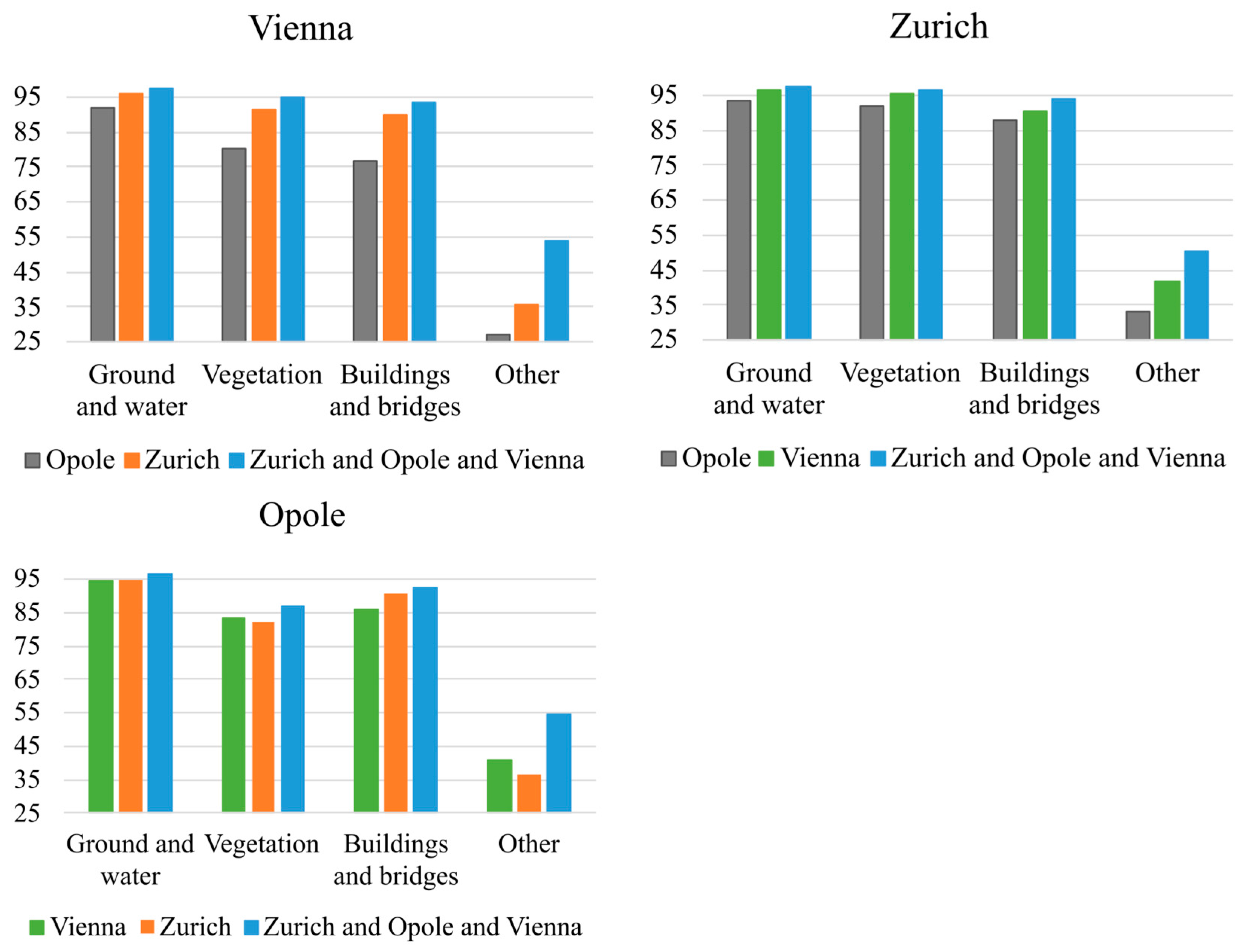
In the case of Experiment 1a, the IoU-defined accuracy for the ground and water class varied between 96.3% and 97.8%, for the vegetation class varied between 86.9% and 96.6%, for the buildings and bridges varied between 91.5% and 93.6%, and for the ‘other’ class varied between 44.7% and 53.5%. For all of the classes except for ‘other’ class, the classifier trained using Zurich data achieved the highest accuracy, whereas the classifier trained using the Opole dataset achieved the lowest accuracy (Figure 9). For the ‘other’ class, the best accuracy was achieved by the classifier trained using the Vienna dataset. However, in most cases (except from vegetation class), the discrepancies are not substantial.
In Experiment 1b, the accuracy of cross-classifiers varied between 91.8% and 96.6% in the case of the ground and water class, 80.0% and 95.2% in the case of vegetation, 76.9% and 90.9% in the case of buildings and bridges, and 27.3% and 41.6% in the case of class ‘other’. The smallest accuracy for all of the experiments was achieved when applying the classifier trained using the Opole dataset on the testing dataset of Vienna. For three out of four classes, the best accuracy was achieved by the classifier trained using the Vienna dataset and applied on the test data of Zurich. However, in the fourth class, the difference between this classifier and the best performing one was equal to only 0.4 pp. In all of the experiments, the classifier trained jointly using all datasets substantially outperformed all of the cross-classifiers (Figure 10). The improvement is especially visible for the class ‘other’.
In Experiment 1c, the achieved accuracy of the joint classifier varied between 96.6% and 97.4% for ground and water, 86.9% and 96.4% for vegetation, 92.5% and 94.0% for buildings and bridges, and 50.4% and 54.6% for the class ‘other’. The visual analysis of the results showed that one of the most commonly occurring errors is the misclassification of shrubs (and crops) as belonging to class ‘other’ instead of vegetation. This is true for both individual shrubs (mostly when their shape resembles a dome) and hedges. This is probably caused by high variability in the shapes of shrubs, inconsistencies in the reference classification, and shrubs being the most problematic class for labeling, even for humans [60]. Moreover, there was a misclassification of both small and horizontal and high (vertical) objects belonging to class ‘other’ as vegetation. This is especially common when a lamp post is located in hedges or very close to them or close to trees. There is often misclassification between hedges and fences. However, this distinction is sometimes impossible to be made even by a human. Moreover, the training data are often inconsistent in terms of the classification of these objects, which in turn leads to the confusion of the models. Another commonly occurring error is connected with the classification of bridge decks that are often classified as ground instead of buildings and bridges. Moreover, the arbitrary border between the bridges/viaducts and ground assumed in training data causes the accuracy of the bridge and viaduct classification to be lower. The last type of error is that, commonly, part of the roof of a large building is classified as ground. The typical error for the Vienna dataset is the classification of urban furniture on viaducts as ‘other’ instead of buildings and bridges (correct classification according to reference). These kinds of errors are caused by differences between reference classifications in Vienna (everything on a viaduct is a building) and in Zurich (objects on top of a viaduct belong to a class typical to this object). However, the classifier consistently classifies urban furniture as ‘other’ regardless of its location (ground or viaduct).
The achieved results show that for all of the conducted investigations, the accuracy of the joint classifier (that was trained simultaneously on all training datasets) was comparable or slightly better than the accuracy of the classifier trained and tested on a single city. The joint classifier tends to keep the accuracy of the ground and water class and of the vegetation class (a difference of maximum 0.4 pp) while improving the accuracy of buildings and bridges, and ‘other’ classes (improvement by a maximum of 1.1 pp and 9.9 pp for buildings and bridges and ‘other’ classes, respectively). The exception is the Zurich dataset, for which the accuracy of these classes was also preserved but not improved (Figure 10).

3.3. Experiment 2

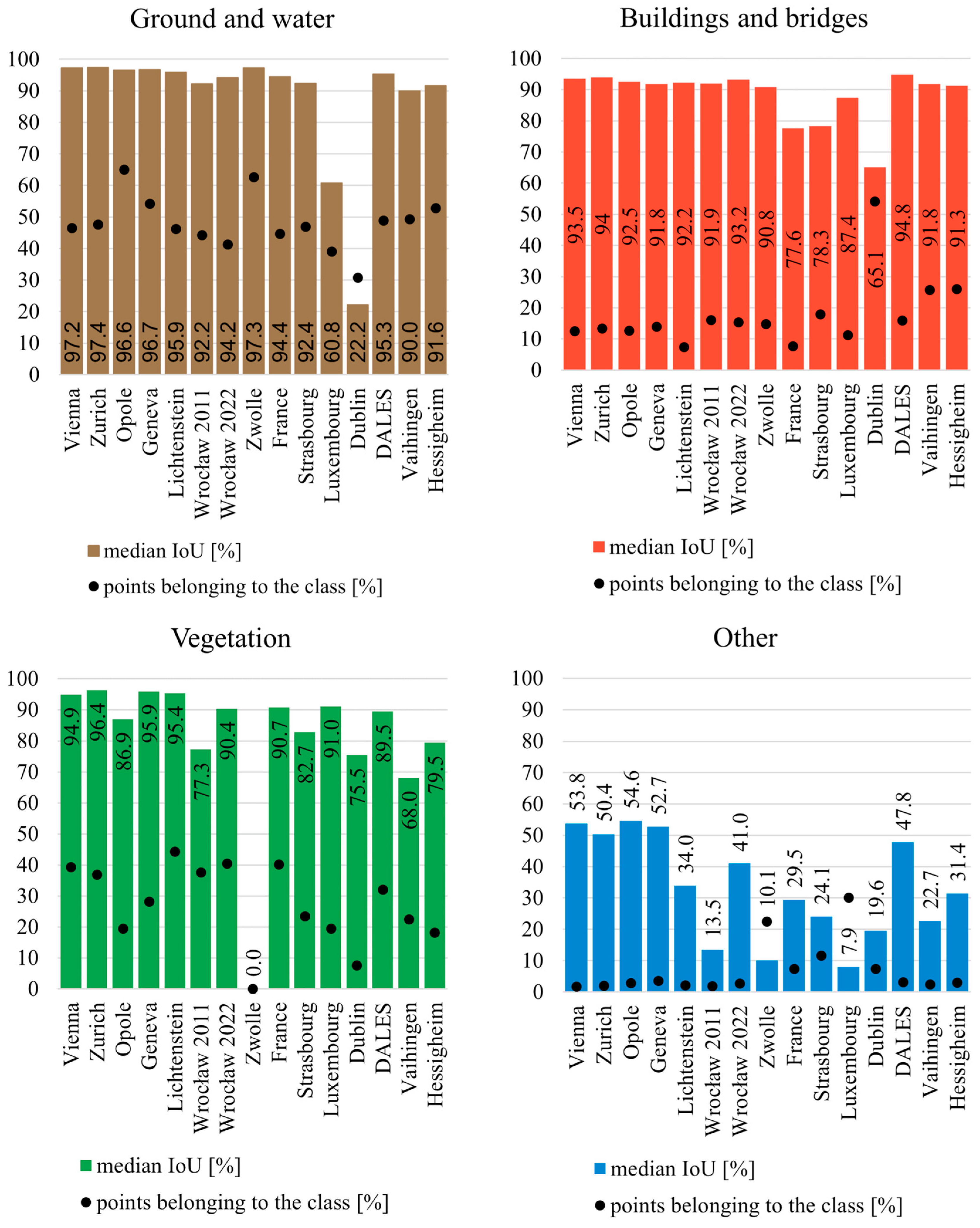
The results of Experiment 2 are presented in Table 4 and Figure 11. The accuracy of semantic segmentation for the DALES dataset does not include one of the tiles where the reference classification was not correct. Moreover, as described in Section 2.1.3, some of the datasets might not be appropriate for the evaluation of the accuracy of each class (see Figure 5).
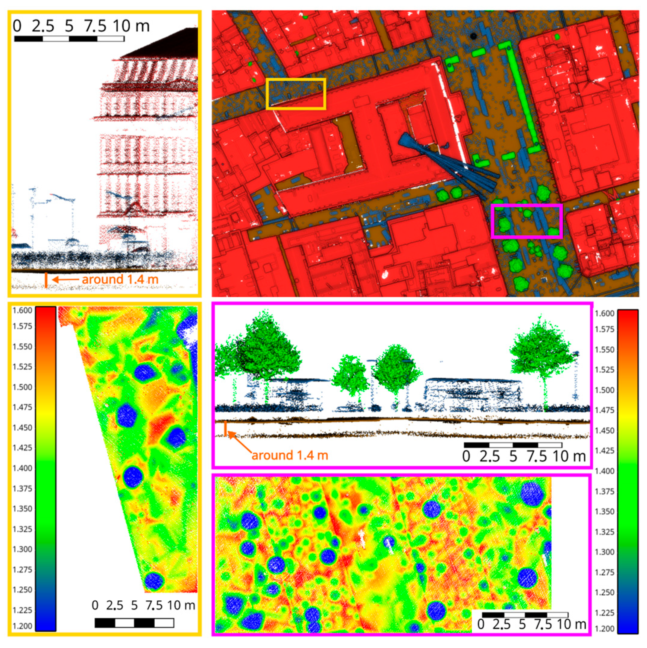
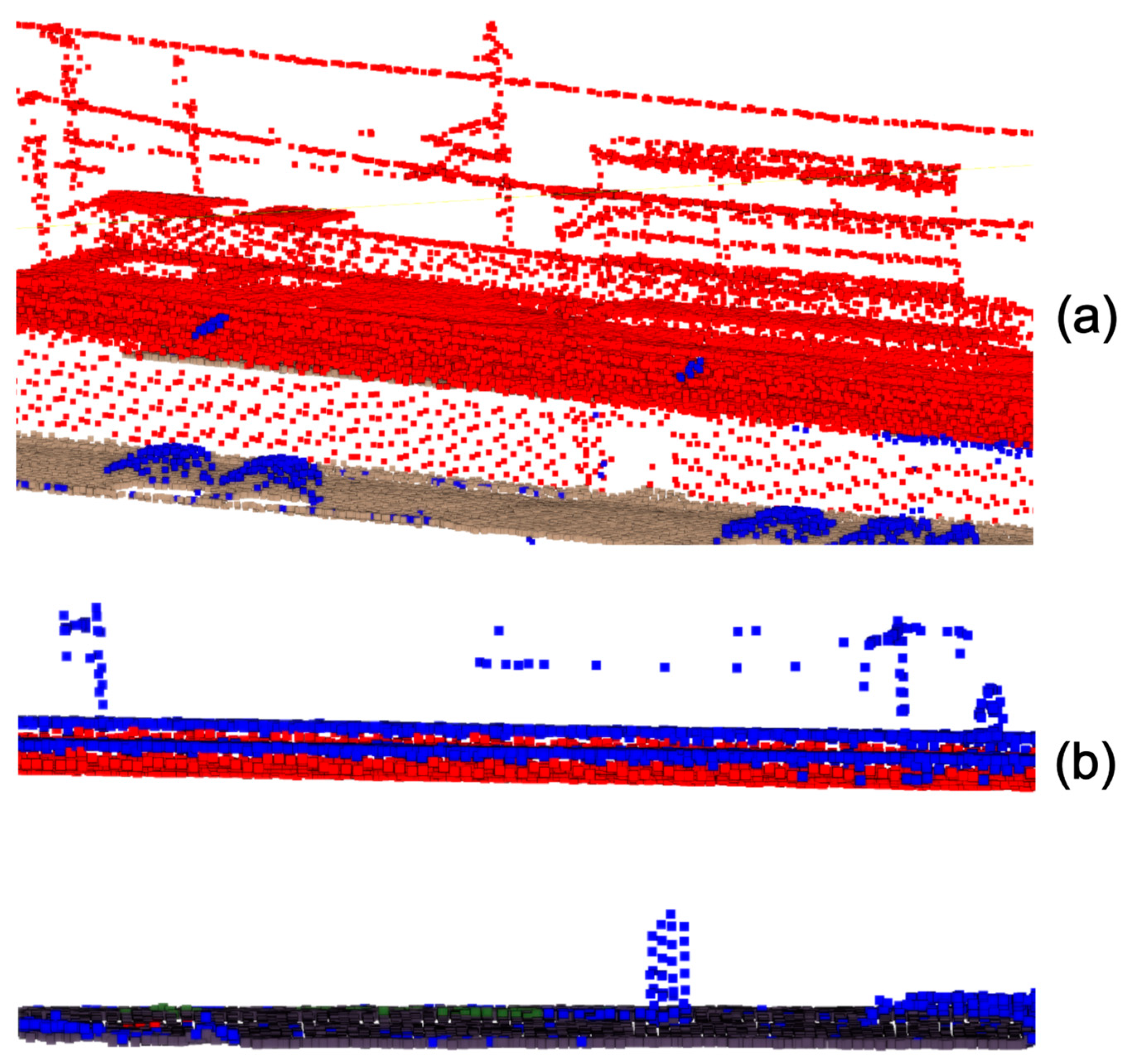
The IoU-based accuracy of the ground and water class varied between 92.2% and 96.7% for dataset A, 92.4% and 97.3% for dataset B, and 90.0% and 95.3% for dataset C. The accuracy of semantic segmentation could not be evaluated for the Dublin dataset, due to geometrical errors in the point cloud (Figure 12), and the Luxembourg data, due to the misclassification of part of the ground points in the reference data (Figure 13).
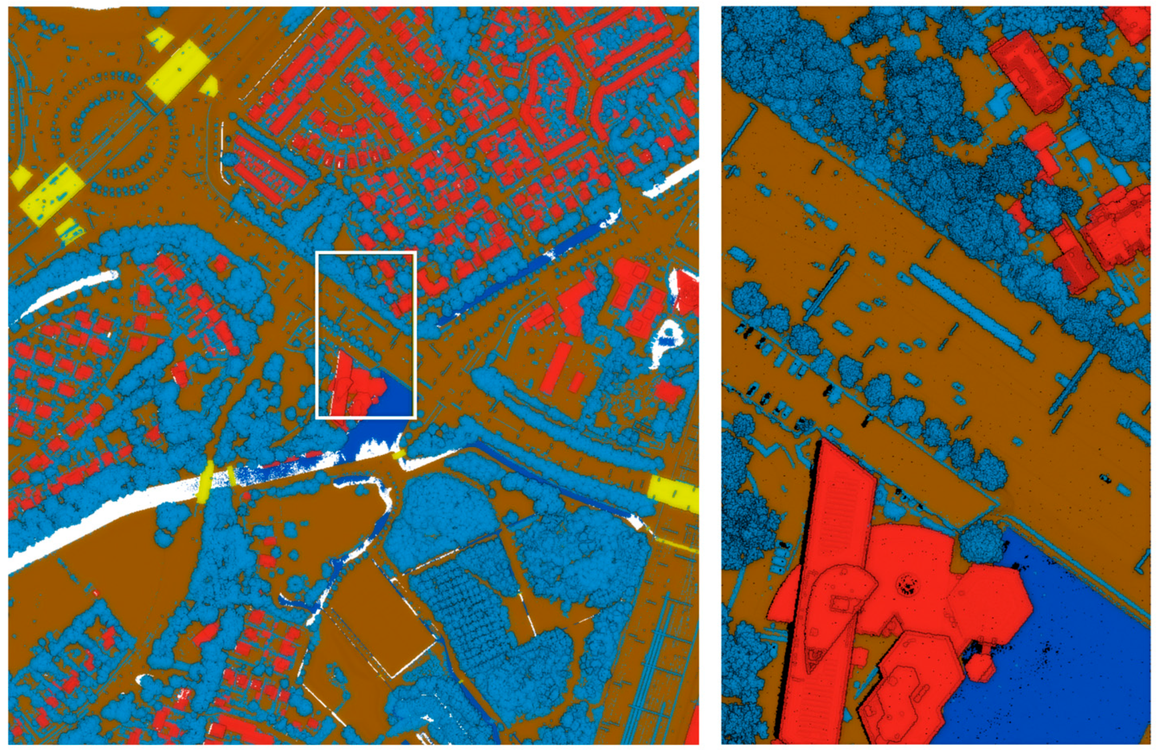
The IoU-based accuracy of the vegetation class varied between 77.3% and 95.9% for dataset A, 82.7% and 91.0% for dataset B, and 68.0% and 89.5% for dataset C. The accuracy of the vegetation class could not be evaluated for the Zwolle dataset, due to the lack of this class in the AHN3 data (Figure 14), and the Dublin data, due to geometrical errors in the point cloud (Figure 12).
The IoU-based accuracy of buildings and bridges varied between 91.8% and 93.2% for dataset A, 77.6% and 90.8% for dataset B, and 91.3% and 94.8% for dataset C. The Dublin (dataset C) and Strasbourg (dataset B) datasets could not be used for the evaluation of the accuracy of semantic segmentation for this class due to geometrical errors in data (Dublin) and the lack of facades in the buildings class (Strasbourg) (Figure 12 and Figure 15).
The IoU-based accuracy of the ‘other’ class varies between 13.5% and 52.7%. The data from Luxembourg and Zwolle (dataset B) could not be used for the evaluation of the accuracy of this class as they present a classification scheme in which the ‘other’ class includes facades and vegetation, respectively (Figure 13 and Figure 14).

4. Discussion

4.1. Choice of Classes and Data

In the publication [61], Roscher et al. introduce the term “data-centric learning”. They argue that the performance of many machine learning methods has already saturated on benchmark datasets in remote sensing. It becomes more important to focus on “data creation”, “data curation”, and the “evaluation” of the results, than to focus on “model training”. They close the machine learning cycle by “development and feedback” to the starting point of “problem definition”. In this respect, our contribution concentrates on “problem definition”, “data curation”, and “data evaluation”. Concerning the topic of saturation, the methods presented in Section 1.1.2 reached an overall accuracy in their benchmark studies between 96% and 98% for two-class problems (two results), mostly between 90% and 98% for four- or five-class problems (six of seven results), and mostly between 80% and 85% on nine- or eleven-class problems (seven of eight results).
The choice of the classes ‘building and bridges’, ‘vegetation’, ‘ground and water’, and ‘other’ was governed by classic land covers found in Earth observation. Outside city areas, i.e., outside our focus areas, different land covers (glacier, swamp, etc.) may become very important, and this is also reflected in the USGS standard for the classification of LiDAR data [62] which consists of seven classes. However, in that scheme, urban areas constitute only one class. On the other hand, the Copernicus global land cover map [63], which is based on optical and radar satellite remote sensing, includes 12 classes. In this scheme, the land cover class “Built-up” includes buildings, man-made structures, and roads. With the much higher resolution of LiDAR data, finer classification schemes are possible, but as Figure 1 shows, there is no common understanding of which classes these should include.
The choice to include bridges in the building class, as well as to include water in the ‘ground’ class, is a consequence of this heterogeneity. We note that the water portion in the ‘ground and water’ class, and even more, the portion of bridges in the ‘building’ class is very low. According to the Vienna datasets, these are 1.9% and 1.4%, respectively. It is further noted that using segmentation (e.g., [64]) and/or additional data sources, e.g., OpenStreetMap (e.g., [65]) can be used to support the identification of water within this class.
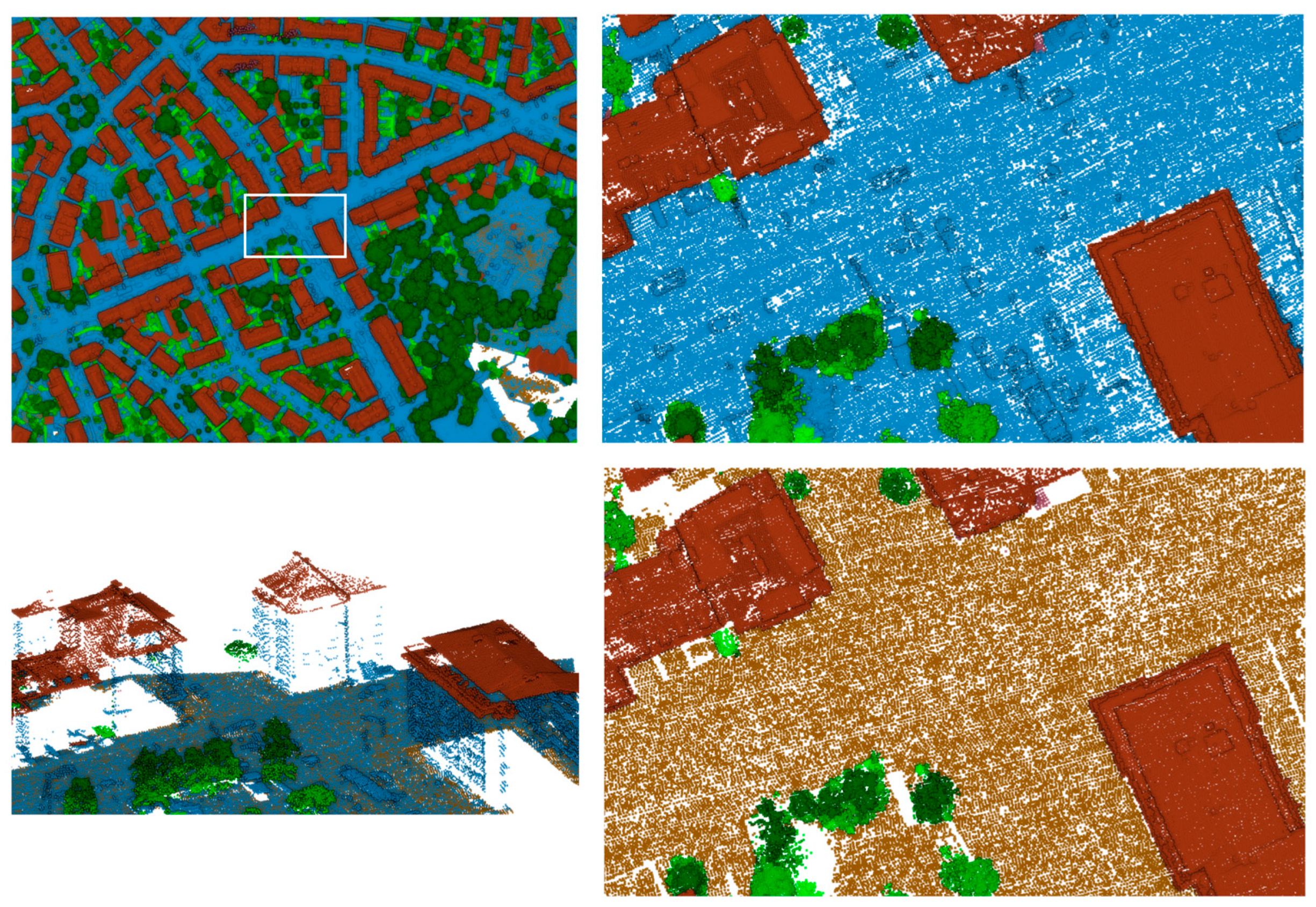
The class ‘other’ comprises diverse urban elements. Some inconsistency of reference class labels could not be entirely avoided. One such example is street furniture on viaducts. In the Vienna dataset, these are in the class buildings and bridges, whereas in the Zurich dataset they are in the class ‘other’ (Figure 16). Correspondingly, those elements ended up in our training and testing datasets in the classes ‘buildings’ and ‘others’, respectively.
While it is possible that some of the applications of ALS point clouds could benefit from the finer classification scheme, it is also important to keep a balance between the simplicity of a scheme and the applicability of the resulting classified point clouds and to take into account the current availability of the datasets.

4.2. Model Performance

The results of tests performed for hyperparameter adjustments showed that increasing the number of convolutional layers or number of iterations did not cause major improvements in the model accuracy. However, lowering the number of iterations, increasing the voxel size, lowering the number of convolutional layers, lowering the number of features generated by each convolutional layer, and using a non-weighted loss function caused a noticeable drop in the accuracy of the model. Therefore, it can be concluded that the baseline set of hyperparameters is well adjusted to the problem at hand.
In Experiment 1a, the classifiers achieved generally high accuracy varying between 86.9% and 97.8% for ground and water, vegetation, and building and bridges classes. Lower accuracy was achieved for the class ‘other’, which is caused by an underrepresentation of this class in the training data, high variability of objects in this class, and lower accuracy of the reference classification for this class in all datasets. For most of the classes, the best accuracy was achieved for the Zurich dataset, whereas the lowest accuracy was reported for Opole data. However, usually the accuracy achieved for Vienna data is only slightly lower than in the case of Zurich. The Opole dataset achieves an accuracy comparable to other datasets for ground and water as well as buildings and bridges classes. However, the accuracy of the vegetation and ‘other’ classes is lower. This can be caused by two reasons: a much lower percentage of vegetation points in the Opole data in comparison to the Vienna and Zurich datasets and a lower accuracy of reference classification for the Opole dataset. Nevertheless, the accuracy achieved by all classifiers is satisfactory.
The results of Experiment 1b show that the classifier trained using Opole data achieves lower accuracy when scaled to other datasets than the classifiers trained using Zurich and Vienna datasets. However, the differences between Vienna and Opole classifiers achieved when processing Zurich data are not substantial (except for the ‘other’ class). Bigger differences can be observed when Zurich and Opole classifiers are used for processing Vienna data. This can be caused by more similarities between Opole and Zurich as they are more similar in terms of the size of the city, which also influences the type of the buildings and amount of vegetation in the city. On the other hand, the cross-classifiers trained using Zurich and Vienna data tend to perform similarly when applied to Opole data. They also achieve higher accuracy than the model trained using Opole data when applied to Zurich and Vienna datasets. This can be caused by a smaller number of points and smaller coverage area of the Opole dataset in comparison to other datasets and by different class frequencies for this dataset.
The results of Experiment 1c show that, in most cases, the joint classifier enabled the accuracy of each of the individual classifiers to be kept, while allowing for the improvement of certain classes. For instance, in the Vienna data, the joint classifier enabled an improvement of the accuracy of the buildings and bridges class by 1.1 pp. The visual inspection of the point cloud showed that by joining the datasets, it is possible to reduce building classification errors caused by the misclassification of the middle parts of flat roofs of large buildings. Moreover, it prevented many cases of misclassification of the ground around buildings as buildings. However, most improvements are related to the classification of buildings, whereas the accuracy of the semantic segmentation of bridges is usually lower for the joint classifier, which can be caused by higher variability in types of bridges introduced to the classifier by joining the datasets. Another example of improvement is the higher semantic segmentation accuracy achieved by a joint classifier for the ‘other’ class in the Opole dataset (improvement by 9.9 pp).
These results of Experiment 1c show that joining multiple datasets for the training of the classifier has a positive influence on the accuracy of semantic segmentation. Moreover, together with the results of Experiment 1b, they suggest that the joint classifier is able to accurately classify a higher variety of datasets than the classifier trained only on one city, which in turn proves the higher generalizability of the achieved model. The improvement in the generalization accuracy is most probably caused by the increase in the amount of training data of different characteristics, which in turn leads to the inclusion of a larger number of objects of very different characteristics and minimization of the influence of the errors typical for one source of the data. Moreover, by joining datasets, we average the frequency of the presence of certain objects, which has an influence on the generalizability of the model as the classifier learns not only the features but also the frequency of the object’s presence in the data.

4.3. Generalization

The generalization of the model was evaluated based on 12 different datasets. The achieved accuracy suggests that the model generalizes well to the previously unseen data. The class-wise accuracies of the test datasets are comparable to the lowest accuracy achieved by a joint classifier for the test dataset of the cities used for training. The median values calculated for each class are 2.3 pp lower in the case of ground and water, 2.6 pp higher in the case of vegetation, 0.7 pp lower in the case of buildings and bridges, and 19 pp lower in the case of the ‘other’ class. However, the higher discrepancy for the ‘other’ class is not surprising as the reference classification differences are higher for this class too. We can also expect that the variability of objects that are assigned to this class in different datasets is higher in comparison to other classes and can highly depend on size and location of the city. Moreover, the accuracy of ‘other’ class was lower than the accuracy of other classes even for the classifiers that were trained and tested on the dataset of the same city.
The highest semantic segmentation accuracy was achieved for the Geneva dataset, which was expected, as the data come from the same dataset as Zurich data that were used for the training of the classifier. Moreover, Geneva is located in the same region of Europe as Zurich. Thus, we can expect a similar structure to the city, which affects the results as well. Finally, the source dataset is characterized by extremely high classification accuracy. Consequently, the errors in reference classification do not have a large influence on the evaluation of the classifier. The above conclusions can be supported by the similarly high accuracy of the Liechtenstein dataset that is also a part of Swiss national data but represents an area with slightly different characteristics for the terrain and buildings.
A very good accuracy was also achieved for the DALES dataset. It represents a smaller area than the national datasets but it is still large in comparison with the usual size of benchmarking datasets. In the case of this kind of dataset, the creators pay additional attention to the accuracy of reference classification. This means that we can safely omit the influence of reference classification inaccuracy on the results of the evaluation of the classifier. The data represent a city outside of Europe, and thus the similarity of the objects present in the point cloud may be smaller than in the other datasets. Moreover, there should not be many similarities in the equipment used, as the data were acquired independently from training data. On the other hand, the complexity of the objects included in the point cloud may be smaller than in the case of European datasets that represent densely populated cities. Since the similarities between the DALES dataset and training data are very small, the reference accuracy of classification is expected to be high and the spatial coverage of the dataset is substantial; the accuracy achieved for this dataset can be considered an objective evaluation of the accuracy of a joint classifier.
The lower accuracy for the Wrocław 2011 dataset might be caused by several reasons. First, the dataset was acquired and preprocessed much earlier than all of the training samples. As a result, we can expect that the methodology of the creation of reference classification, the density of the point cloud, and the equipment used may differ substantially between the training data and the Wrocław 2011 dataset. Moreover, the accuracy of the reference classification of this dataset is much lower than the reference classification accuracy of other datasets. As a result, its influence on the evaluation of the accuracy of the classifier might be substantial. The results achieved for the same region but for the point cloud collected in 2022 seem to confirm these conclusions, as the achieved accuracy was higher for every class, especially for vegetation. Indeed, the visual inspection of the data confirmed that the reference classification accuracy was higher in the case of newer data. However, it is still not as good as the accuracy of the reference classification of Swiss or Austrian data, which suggests that the real classifier accuracy might be slightly different than the results reveal.
The smallest accuracy was achieved for the Vaihingen dataset. Vaihingen is a benchmarking dataset and we can expect it to be characterized by a very high accuracy of reference classification. As a result, the influence of this factor on the evaluation results can be disregarded. However, the Vaihingen point cloud was collected much earlier than the training point clouds and has a very small point density. Moreover, the spatial size of the dataset is extremely small. As a result, any error during semantic segmentation has a strong influence on the final result. A lower accuracy can be observed, especially for the vegetation class, which is caused by an overrepresentation of shrubs in the dataset. Since the tested classifier was trained using national datasets, it is not able to achieve a high accuracy of semantic segmentation for shrubs. This is because of reference classification errors that are quite common for these kinds of objects and because of their underrepresentation in the most common city scenarios. Better semantic segmentation accuracy can be observed for the Hessigheim dataset, which has higher point density. The difference is especially visible for the vegetation class. However, the Hessigheim data also cover a very small area, which contains large amounts of shrubs, which is not the typical case for most city areas.
Nevertheless, the results of the experiments prove that the classifier is able to generalize between the datasets of different sources and characteristics while keeping high semantic segmentation accuracy. However, there is still room for improvement, especially in the case of the classification of shrubs (vegetation class). This would require more datasets with a high accuracy of reference classification and a similar classification scheme to the currently used training datasets.

4.4. Quality of Data and Labels

The quality of training and testing data has a major influence on the accuracy of developed deep learning models [66]. In the case of point clouds, data quality can be understood both as the geometrical quality of the point clouds and as the quality of the reference labels provided for each point. The available point cloud datasets, both benchmarking and national, are characterized by very different qualities depending on their source.
When it comes to the geometrical accuracy, in the process of training and testing the classifier we make two assumptions: (1) the used point clouds are free of errors coming from data acquisition and processing, and (2) the data do not represent contradicting scenes. The first assumption may be violated when the strip adjustment is not performed for the point cloud, whereas the second assumption is not valid when the analyzed area represents, e.g., a construction site and consists of point clouds collected during different times.
These assumptions are not fulfilled in the case of the Dublin dataset where the point cloud shows geometrical errors, such as two layers of ground level (Figure 12). As a result of the assumptions above, the classifier correctly learned that there can be only one level of ground, which led to the misclassification of a higher layer of ground as a building. To confirm that the lower accuracy of the semantic segmentation for this dataset was achieved due to this geometrical error, we performed an additional experiment. We randomly selected two tiles of the data and manually removed the lower ground level from the point cloud. Then, we evaluated the accuracy of semantic segmentation for these tiles. The IoU-based accuracy of the ground and water class for these tiles improved from 42.9% to 88.5% and from 8.7% to 84.6%. Moreover, in both cases, the accuracy of all of the other classes improved as well, by up to 5.9 pp in the case of vegetation, 25.1 pp in the case of buildings and bridges, and 15.5 pp in the case of the ‘other’ class. This proves that the presence of two levels of ground had a substantial influence over the accuracy achieved for this dataset, not only for the ground and water class but also for other classes in the dataset. Therefore, the Dublin dataset could not be used for the evaluation of the model performance in the case of building and bridges and ground and water classes. Moreover, it can be expected that the accuracy of the vegetation class and the class ‘other’ would improve as well if the data were geometrically error-free.
Another type of data quality is the quality of the provided reference labels. The review of the existing ALS datasets proved that many of them are characterized by high reference classification error. At the same time, the semantic segmentation accuracy metrics do not take into account the reference label errors present in the dataset. Therefore, they need to be taken into account during the analysis of the results. In [66], it is suggested (in the context of object detection in 2D images) to use multiple annotations of the same object, to measure “label convergence”. This defines an upper bound for the quality measure that can be obtained when testing the classifier.
The performed experiments suggest that the accuracy of reference classification has a major influence on the accuracy of the joint classifier, both in the training and testing stage. The classification errors present in the training data may lead to training the classifier to make the same mistakes as were present in the training data. Since it is impossible to prepare training data that do not contain any errors (even in the case of small, benchmarking datasets), the fusion of data that comes from different sources creates a possibility to train a classifier to disregard data-specific errors and focus on common patterns between the datasets. As a result, training datasets can complement each other in terms of error propagation as well as the presence of objects specific for a region and characteristics of the acquired data. As suggested in [66], we took utmost care to select only the best datasets for training because there is a certain danger that deep neural networks can be affected by overfitting, and thus reproduce label errors of the reference data. We argue that the optimization process and the normalization of the data during the training phase, together with the large, diverse, and high-quality data volume of our approach, prevents this. This argument is supported by the analysis of Opole. This dataset obviously has the highest number of reference label errors and training only from this dataset leads to the lowest ranking results. The joint classifier, on the other hand, is not only the overall best, but also the best on the Opole data. That the performance on Opole is still lower than on Vienna or Zurich is a matter of the lower quality of the reference data. On the other hand, the classification errors present in the testing datasets make it difficult to objectively evaluate the accuracy of the classifiers. The existing datasets are usually small benchmarking datasets where additional attention was paid to create accurate labels or large, national datasets where, due to their size, it is not possible to sustain as high of an accuracy of the reference classification as in the case of benchmarking datasets. However, the latter ones provide more opportunities in terms of the variability of objects, types of neighborhoods (e.g., city centers, suburbs, forests, parks, etc.), and data characteristics (e.g., point density).
Taking into consideration the above conclusions, it can be expected that the accuracy achieved for test sets of Vienna, Zurich, Opole, and other cities that belong to Swiss data (Geneva and Liechtenstein) is slightly overestimated, as the errors that occur in the reference classification of these datasets are similar to the ones present in the training data. On the other hand, the accuracy achieved for other datasets (national and benchmarking) is underestimated, as the errors in the reference data are likely different from the ones present in the training data.

4.5. Comparison to the Literature

A comparison of the results achieved by the joint classifier with the results presented in the literature constitutes a challenging task due to the following reasons:
  • The experiments in the literature are performed using various national ALS datasets, but they are mostly considering AHN point clouds, whereas in the investigations presented in this paper, this dataset could not be fully used due to significant differences in classification schemes.
  • A lack of standardization in terms of classes into which the data are classified. As a result, different investigations propose a different set of classes that usually depend on the classification scheme of the reference data. Since the number of classes influences the values of the metrics describing the accuracy of semantic segmentation, in this case, the results cannot be reliably compared.
  • A lack of standardization in terms of metrics used for accuracy evaluation. The most commonly used metric seems to be the F1 score. However, sensitivity, precision, and IoU are also often used.
  • The test set of benchmarking datasets is often not available for a direct comparison and requires sending a classifier to the organizers.
  • Even when the publications use the same national dataset, they present the results using different parts of the dataset (e.g., different geographical location).
Nevertheless, we performed an analysis that enabled us to roughly compare the achieved results with state-of-the-art approaches. For this purpose, we recalculated our results to the F1 score metric using precision and recall values (see Appendix B, Table A2).
Table 5 presents the semantic segmentation results of the test set from the Vaihingen dataset, as reported in various selected literature sources. We decided to use the results reported in the literature rather than the results described on the competition website as the accuracies reported in literature show the most recent development of the models. It is not possible to directly compare these results for three reasons: (1) in our research, we use a smaller set of classes, which positively affects the accuracy; (2) we do not train our model using the training set of the Vaihingen data, which should negatively affect the accuracy; and (3) since we do not use Vaihingen for training, we used all of the data (training and testing sets) in order to evaluate the results. However, we can conclude that the achieved results do not stand out from state-of-the-art accuracies. In the case of all of the classes except the ‘other’ class, the achieved accuracy reaches the highest values achieved by the classifiers trained using the Vaihingen dataset. The accuracy of ‘other’ class still fits in the accuracy ranges reported in the literature but it is more in the middle of the reported ranges. Based on this comparison, we can conclude that the joint classifier achieving a lower accuracy for the vegetation class for the Vaihingen dataset in comparison to other testing datasets does not indicate weak generalization of the classifier but rather the specificity of the Vaihingen dataset. Moreover, it seems that the difficulties with the classification of shrubs observed for the joint classifier are also typical for machine learning tasks, as the reported accuracy of this class is lower than most of the other classes. The lower accuracies of the ‘other’ class also seem to be typical for the semantic segmentation tasks due to the high variability of objects in this class.
The classification scheme most similar to ours was used in [16], where the accuracies achieved by a model trained using the Vaihingen dataset are comparable to the accuracy of the joint classifier. Moreover, in [16], the cross-validation accuracy was investigated for the model trained using the LASDU dataset and evaluated using the Vaihingen dataset. However, in this case, the reported accuracies are lower than the accuracy of the model trained using the Vaihingen dataset. These accuracies are, in turn, substantially lower than the accuracy of a joint classifier for this dataset, which indicates higher generalization capabilities of the joint classifier.
Table 6 presents the results reported for the ALS part of the Hessigheim dataset shown on the competition website. Unfortunately, most of the investigations are performed for UAV LiDAR, not ALS. However, the website presents the results of three approaches. The results achieved by the joint classifier cannot be directly compared as we use training and validation data (the test data are not publicly available as this is an ongoing competition) to test the accuracy and we perform the semantic segmentation into four classes instead of eleven. However, the results can be roughly compared. The achieved results usually fall in the accuracy ranges reported in Table 6. The accuracy of ground and water exceeds the accuracies of the classes that are assigned to it. However, this is probably caused by a smaller number of classes. The accuracy of the ‘other’ class is in the lower boundary of the accuracies of vehicles, urban furniture, and vertical surfaces. At the same time, the accuracy of the vegetation class seems to be slightly lower than the accuracy of trees reported on the website but much higher than the accuracy of shrubs. However, this can be caused by a small number of reported accuracies for ALS data. When compared to more commonly reported results for UAV LiDAR semantic segmentation, the vegetation accuracy achieved by our model is well in the middle of the accuracies of trees achieved by the classifiers trained using the Hessigheim dataset, which indicates that the lower accuracy of the joint classifier achieved for the vegetation class for this dataset in comparison to other test datasets does not prove low generalization capabilities of the classifier but rather the specificity of the dataset.
The national dataset that is most commonly used for training and evaluating deep learning models is the AHN dataset. Since this dataset covers the whole country of the Netherlands, usually the achieved results are not comparable, as selected training and testing areas might be different. The accuracies reported in these areas in the literature vary between the following:
(1)
94.2% and 97.5% for ground;
(2)
40.3% and 95.3% for water;
(3)
87.7% and 94.5% for buildings;
(4)
31.5% to 49.1% for civil structures;
(5)
and 86.9% to 94.9% for other.
When comparing the results achieved by the joint classifier for the AHN3 dataset (Zwolle), only ground and water and building and bridges can be taken into account. In the case of ground and water and building and bridges, the achieved accuracy exceeds the accuracies reported in the literature, even for the investigations that use a limited number of classes. It is not possible to compare the ‘other’ class with the accuracies achieved in the literature. However, the class ‘other’ reported in the literature can be roughly compared to the vegetation class, as it mostly contains points belonging to the vegetation. As a result, it can be concluded that the joint classifier achieves an accuracy comparable to the ones reported in the literature for classifiers trained and tested using the same dataset.
Another example of the national dataset that was used in the literature is the Vienna dataset [9]. The results reported in the literature are comparable with the accuracies achieved by the joint classifier for Vienna, Zurich, and Opole datasets with a slightly smaller accuracy of vegetation for the Opole dataset. However, this might be caused by the smaller reference classification accuracy of the Opole dataset in comparison to the Vienna data. For the other national datasets, the accuracy is comparable for ground and water and buildings and bridges classes and slightly lower for vegetation. The biggest difference can be observed for the class ‘other’. However, this is an expected outcome.
To sum up, the results achieved by a joint classifier are usually comparable to the accuracies achieved in the literature, even when compared to the models trained and tested using the same dataset. However, the results could not be precisely compared due to differences in classification schemes and datasets used.

4.6. Future Research

The accuracies achieved by a joint classifier both for datasets used for training and previously unseen data are very promising. However, there is still room for improvement, especially in terms of the classification of vegetation. This could be tackled by introducing more high-quality data to the training of the classifier. The availability of such data is very limited at the time. However, in the future, more well-classified datasets can be published. Therefore, in the future, it might be beneficial to test the influence of including more thoroughly labeled datasets in the training set. This refers to the “accuracy” of the training data in the terminology of data-centric machine learning [61].
The main factor limiting the applicability of numerous available ALS datasets is the quality of reference classification. Thus, future research could focus on how to utilize existing datasets provided with erroneous classifications. This could potentially include using methods for training with errors or including unlabeled data in training sets. Additionally, there is a need for better understanding of how these errors would influence the model performance and scalability. Recently many synthetic point cloud generation methods have been developed, which raises the opportunity to use synthetic data for training the model and possibly enhancing its scalability. In this case, it is important to find whether the synthetic dataset can improve the scalability of the models and, if so, understanding what ratio of synthetic to real data best serves the model accuracy. It could also be interesting to investigate how unsupervised domain adaptation techniques can be used together with transfer learning for improving the generalizability of the model to the selected datasets. The efforts put into the development of the best scalable classifier should take into consideration both the accuracy of the model and computation time. Since the main goal of this paper is to develop a model that will not have to be retrained before applying it to new data, it is the inference time of the model that should be of main importance. We believe that investigating these areas should also lead to the improvement of the scalability of the model. In this paper, we evaluated how one implementation of the deep network—SparseConvNet—reacts to using multiple datasets for the training of the classifier. However, it would also be beneficial to investigate whether the conclusions would be the same in the case of other architectures, such as PointNet++ or DGCNN. In this sense, we see a need for methodological development.
The investigations presented in this paper aimed at the semantic segmentation of ALS data only. Moreover, the data were mostly collected in Europe. However, the problem of the development of a scalable deep learning model can be analyzed more generally in the context of both the geographical location and sensor used. Therefore, future research could also aim at extending the training data with point clouds representing different geographical locations and acquired with different sensors (terrestrial, mobile, UAV LiDAR, and photogrammetric point clouds), thus increasing training data “diversity and completeness” [61].
In order to become a widely accepted standard, effort should be made to achieve more finely-grained classifiers. However, this requires high-quality training data of a sufficient amount and variability. An obvious step is to distinguish between ground and water, although the special properties of the appearance of water in ALS point clouds (absorption, mirror-like reflection, etc., occurring in the measurement process) complicate the generation of a diverse and complete dataset.

5. Conclusions

In this paper, we investigated the possibility of training a deep learning-based classifier so that it generalizes well to previously unseen data. To achieve the goal, we proposed training the model by jointly using multiple ALS datasets published by various European countries. Since these datasets were collected independently, their characteristics vary substantially. However, while the available datasets are usually classified, the accuracy of the classification of most of them is not good enough for training the model. Therefore, we investigated available ALS datasets with a focus on the accuracy of their classification, and for the training of the model, we selected the point clouds acquired for Austria, Switzerland, and Poland as they are characterized by a higher than usual classification accuracy. Since the data are acquired independently by each country, there are substantial differences in the classification schemes of these point clouds. Thus, we conclude that it would be beneficial to develop a standard of a common minimum set of classes that can be applied for all of the European ALS datasets. As a baseline, we suggest the classes ground and water; vegetation; building and bridges; and other.
The developed classifier is based on a SparseCNN implementation of a three-dimensional, convolutional neural network. The performed experiments proved that it is possible to mix the existing national ALS datasets in order to train a classifier. The joint classifier, trained using the ALS data from Poland, Austria, and Switzerland together, enables the accuracy of the classifiers trained using individual datasets to be kept and, in some cases, even improves these results. In comparison to models trained using only one data source, the model is characterized by higher generalizability. Moreover, the testing results revealed that the joint classifier is able to accurately classify both data that come from the same source as training datasets and new, unobserved datasets that come from national point clouds published by other countries and from benchmarking datasets.
However, when the national datasets are used both in the case of training and testing, the reference classification inaccuracies need to be taken into account as it is impossible to obtain faultless reference classification for such a large area. These errors make it very hard to objectively measure the accuracy of the classification of the datasets from different countries. At the same time, most of the more accurate benchmarking datasets cover a very small area and do not represent the variability of objects that may occur in the point clouds. As a result, the evaluations of the accuracy are biased by the uncertainty of the reference classification and unrepresentativeness of the benchmarking datasets. Using IoU (intersection over union) as an accuracy measure, we argued that the DALES dataset used in testing is a not an overly optimistic estimation of accuracy. The “universal” classifier achieved 95% for ground and water, 90% for vegetation, 95% for building and bridges, and 48% for the class ‘other’.
The availability of a classifier trained using a large-scale dataset together with a thorough validation of its scalability will enable a faster and cheaper semantic segmentation of ALS data, which in turn could lead to better quality of available spatial data. It can also be used as a pretrained model in transfer learning and domain adaptation methods. The thorough validation of the model’s performance on various datasets outlines the expectations that potential users can have when deciding to use it. Moreover, the existence of a model that can be easily used has potential for helping and accelerating the process of the standardization of point cloud classification schemes among various available datasets. This, in turn, will lead to a higher usability of the data and to a higher comparability of the results obtained for investigations that employed large-scale point clouds.

Author Contributions

Conceptualization, A.W. and N.P.; methodology, A.W. and N.P.; software, A.W.; validation, A.W.; formal analysis, A.W.; writing—original draft preparation, A.W.; writing—review and editing, A.W. and N.P.; visualization, A.W.; supervision, N.P.; funding acquisition, A.W. All authors have read and agreed to the published version of the manuscript.

Funding

This research was funded by National Science Center, Poland in the frame of grant number UMO-2021/41/N/ST10/02996.

Data Availability Statement

The code and trained classifier are openly available at https://github.com/AgataWalicka/Universal-Classifier. Further inquiries can be directed to the corresponding author.

Acknowledgments

This article is a revised and expanded version of a paper entitled Semantic Segmentation of Buildings Using Multisource ALS Data, which was presented at the 3DGeoInfo conference in Munich, 12–14 September 2023.

Conflicts of Interest

The authors declare no conflicts of interest.

Appendix A

The methodology of class reassignment for the purpose of testing the generalization of the developed joint classifier (Table A1).
Table A1. Class reassignment methodology.
DatasetOriginal ClassificationReassigned Classification
ViennaGroundGround and water
VegetationVegetation
BuildingsBuilding and bridges
WaterGround and water
BridgeBuilding and bridges
Noise
OtherOther
Zurich
Geneva
Liechtenstein
GroundGround and water
VegetationVegetation
BuildingsBuilding and bridges
Bridges and viaductsBuilding and bridges
WaterGround and water
OtherOther
Opole
Wrocław 2011
Wrocław 2022
GroundGround and water
Low vegetationVegetation
Medium vegetationVegetation
High vegetationVegetation
Buildings and bridgesBuilding and bridges
High points
Low points
WaterGround and water
OtherOther
ZwolleGroundGround and water
BuildingsBuildings and bridges
Civil structuresBuildings and bridges
WaterGround and water
OtherOther
FranceGroundGround and water
Low vegetationVegetation
Medium vegetationVegetation
High vegetationVegetation
BuildingsBuildings and bridges
WaterGround and water
BridgeBuildings and bridges
Perennial soilGround and water
Noise
Virtual points
OtherOther
StrasbourgGround and waterGround and water
Building roofsBuildings and bridges
VegetationVegetation
BridgesBuildings and bridges
Pylons and cablesOther
OtherOther
LuxembourgGroundGround and water
Low vegetationVegetation
Medium vegetationVegetation
High vegetationVegetation
BuildingsBuildings and bridges
Noise
WaterGround and water
BridgesBuildings and bridges
Power linesOther
OtherOther
DublinBuildingBuildings and bridges
VegetationVegetation
GroundGround and water
UndefinedOther
DalesOtherOther
GroundGround and water
VegetationVegetation
CarsOther
TrucksOther
Power linesOther
FencesOther
PolesOther
BuildingsBuildings and bridges
VaihingenPowerlineOther
Low vegetationGround and water
Impervious surfacesGround and water
CarOther
Fence/hedgeOther
RoofBuildings and bridges
FaçadeBuildings and bridges
ShrubVegetation
TreeVegetation
HessigheimLow vegetationGround and water
Impervious surfacesGround and water
VehicleOther
Urban furnitureOther
RoofBuildings and bridges
FaçadeBuildings and bridges
ShrubVegetation
TreeVegetation
Soil/gravelGround and water
Vertical surfacesOther

Appendix B

Table A2 presents the accuracy of the joint classifier as median precision, recall, and F1 score.
The F1 score results were calculated according to the following equation:
F 1 = 2 · P r e c i s i o n m e d i a n · R e c a l l m e d i a n P r e c i s i o n m e d i a n + R e c a l l m e d i a n
Table A2. Accuracy of the joint classifier evaluated using test datasets independent from the training data. “No data” entries occur in those cases where the test data could not be used for evaluating the corresponding class.
NameCountryGround and WaterVegetationBuildings and BridgesOther
PrecisionRecallF1PrecisionRecallF1PrecisionRecallF1PrecisionRecallF1
ViennaAT98.599.298.897.597.597.597.396.396.868.174.871.3
ZurichCH99.198.598.898.398.198.296.497.79765.371.668.3
OpolePL98.099.198.595.990.092.997.495.596.467.972.670.2
GenevaCH98.398.498.398.097.797.895.596.095.767.374.070.5
LiechtensteinLI97.598.397.997.798.097.895.797.096.357.847.852.3
Wrocław 2011PL94.698.696.698.278.587.395.795.595.615.461.324.6
Wrocław 2022PL96.996.696.796.893.895.395.695.895.746.877.658.4
ZwolleNL97.799.598.694.295.995
FranceFR95.998.997.495.796.596.183.997.890.363.334.144.3
StrasbourgFR92.999.696.188.692.390.4
LuxembourgLU92.698.395.487.899.493.2
DublinIE79.292.485.348.027.034.6
DALESUSA96.598.897.696.193.294.696.997.997.472.859.065.2
VaihingenDE98.091.394.588.277.282.394.896.595.625.083.438.5
HessigheimDE96.794.595.689.288.188.693.897.195.444.052.347.8

Appendix C

Table A3. The IoU-based accuracy of all cross-classifiers.
Training DatasetTesting DatasetIoU
Ground and WaterVegetationBuildings and BridgesOther
MedianMeanStdMedianMeanStdMedianMeanStdMedianMeanStd
OpoleVienna91.888.712.180.075.419.776.965.531.627.329.321.4
ZurichVienna95.994.85.091.690.45.689.783.117.435.737.119.4
Zurich and OpoleVienna91.790.17.989.487.08.285.676.422.317.423.316.9
OpoleZurich93.593.22.792.191.73.587.681.117.833.133.011.1
ViennaZurich96.696.61.495.295.23.090.588.16.641.643.910.4
Vienna and OpoleZurich95.895.71.795.194.53.189.488.36.238.341.511.8
ViennaOpole94.694.31.883.482.07.385.883.86.740.939.211.6
ZurichOpole95.194.32.382.181.48.090.987.77.836.436.613.0
Zurich and ViennaOpole95.194.71.784.082.66.891.287.76.942.041.312.6

References

  1. Kippers, R.G.; Moth, L.; Oude Elberink, S.J. Automatic Modelling Of 3D Trees Using Aerial Lidar Point Cloud Data And Deep Learning. Int. Arch. Photogramm. Remote Sens. 2021, XLIII-B2-2021, 179–184. [Google Scholar] [CrossRef]
  2. Li, M.; Rottensteiner, F.; Heipke, C. Modelling of Buildings from Aerial LiDAR Point Clouds Using TINs and Label Maps. ISPRS J. Photogramm. Remote Sens. 2019, 154, 127–138. [Google Scholar] [CrossRef]
  3. Pađen, I.; Peters, R.; García-Sánchez, C.; Ledoux, H. Automatic High-Detailed Building Reconstruction Workflow for Urban Microscale Simulations. Build. Environ. 2024, 265, 111978. [Google Scholar] [CrossRef]
  4. Park, Y.; Guldmann, J.-M. Creating 3D City Models with Building Footprints and LIDAR Point Cloud Classification: A Machine Learning Approach. Comput. Environ. Urban Syst. 2019, 75, 76–89. [Google Scholar] [CrossRef]
  5. Soilán, M.; Riveiro, B.; Liñares, P.; Padín-Beltrán, M. Automatic Parametrization and Shadow Analysis of Roofs in Urban Areas from ALS Point Clouds with Solar Energy Purposes. ISPRS Int. J. Geo-Inf. 2018, 7, 301. [Google Scholar] [CrossRef]
  6. Zhou, Z.; Gong, J.; Hu, X. Community-Scale Multi-Level Post-Hurricane Damage Assessment of Residential Buildings Using Multi-Temporal Airborne LiDAR Data. Autom. Constr. 2019, 98, 30–45. [Google Scholar] [CrossRef]
  7. Korzeniowska, K.; Pfeifer, N.; Mandlburger, G.; Lugmayr, A. Experimental Evaluation of ALS Point Cloud Ground Extraction Tools over Different Terrain Slope and Land-Cover Types. Int. J. Remote Sens. 2014, 35, 4673–4697. [Google Scholar] [CrossRef]
  8. Chen, C.; Guo, J.; Wu, H.; Li, Y.; Shi, B. Performance Comparison of Filtering Algorithms for High-Density Airborne LiDAR Point Clouds over Complex LandScapes. Remote Sens. 2021, 13, 2663. [Google Scholar] [CrossRef]
  9. Li, N.; Kähler, O.; Pfeifer, N. A Comparison of Deep Learning Methods for Airborne Lidar Point Clouds Classification. IEEE J. Sel. Top. Appl. Earth Obs. Remote Sens. 2021, 14, 6467–6486. [Google Scholar] [CrossRef]
  10. Griffiths, D.; Boehm, J. A Review on Deep Learning Techniques for 3D Sensed Data Classification. Remote Sens. 2019, 11, 1499. [Google Scholar] [CrossRef]
  11. Li, W.; Wang, F.-D.; Xia, G.-S. A Geometry-Attentional Network for ALS Point Cloud Classification. ISPRS J. Photogramm. Remote Sens. 2020, 164, 26–40. [Google Scholar] [CrossRef]
  12. Yousefhussien, M.; Kelbe, D.J.; Ientilucci, E.J.; Salvaggio, C. A Multi-Scale Fully Convolutional Network for Semantic Labeling of 3D Point Clouds. ISPRS J. Photogramm. Remote Sens. 2018, 143, 191–204. [Google Scholar] [CrossRef]
  13. Nurunnabi, A.; Teferle, F.; Li, J.; Lindenbergh, R.; Hunegnaw, A. An Efficient Deep Learning Approach for Ground Point Filtering in Aerial Laser Scanning Point Clouds. Int. Arch. Photogramm. Remote Sens. Spat. Inf. Sci. 2021, XLIII-B1-2021, 31–38. [Google Scholar] [CrossRef]
  14. Rizaldy, A.; Persello, C.; Gevaert, C.; Oude Elberink, S.; Vosselman, G. Ground and Multi-Class Classification of Airborne Laser Scanner Point Clouds Using Fully Convolutional Networks. Remote Sens. 2018, 10, 1723. [Google Scholar] [CrossRef]
  15. Soilán Rodríguez, M.; Lindenbergh, R.; Riveiro Rodríguez, B.; Sánchez Rodríguez, A. Pointnet for the Automatic Classification of Aerial Point Clouds. ISPRS Ann. Photogramm. Remote Sens. Spat. Inf. Sci. 2019, IV-2/W5, 445–452. [Google Scholar]
  16. Widyaningrum, E.; Bai, Q.; Fajari, M.K.; Lindenbergh, R.C. Airborne Laser Scanning Point Cloud Classification Using the DGCNN Deep Learning Method. Remote Sens. 2021, 13, 859. [Google Scholar] [CrossRef]
  17. Wen, C.; Yang, L.; Li, X.; Peng, L.; Chi, T. Directionally Constrained Fully Convolutional Neural Network for Airborne LiDAR Point Cloud Classification. ISPRS J. Photogramm. Remote Sens. 2020, 162, 50–62. [Google Scholar] [CrossRef]
  18. Xie, Y.; Schindler, K.; Tian, J.; Zhu, X.X. Exploring Cross-City Semantic Segmentation of ALS Point Clouds. Int. Arch. Photogramm. Remote Sens. Spat. Inf. Sci. 2021, XLIII-B2-2021, 247–254. [Google Scholar] [CrossRef]
  19. Qin, N.; Tan, W.; Ma, L.; Zhang, D.; Guan, H.; Li, J. Deep Learning for Filtering the Ground from ALS Point Clouds: A Dataset, Evaluations and Issues. ISPRS J. Photogramm. Remote Sens. 2023, 202, 246–261. [Google Scholar] [CrossRef]
  20. Usmani, A.U.; Jadidi, M.; Sohn, G. TOWARDS THE AUTOMATIC ONTOLOGY GENERATION AND ALIGNMENT OF BIM AND GIS DATA FORMATS. ISPRS Ann. Photogramm. Remote Sens. Spat. Inf. Sci. 2021, VIII-4/W2-2021, 183–188. [Google Scholar] [CrossRef]
  21. LAS Specification 1.4-R15; The American Society for Photogrammetry & Remote Sensing: Baton Rouge, LA, USA, 2019.
  22. Walicka, A.; Pfeifer, N. Semantic Segmentation of Buildings Using Multisource ALS Data. In Recent Advances in 3D Geoinformation Science; Springer: Cham, Switzerland, 2024. [Google Scholar]
  23. Bello, S.A.; Yu, S.; Wang, C.; Adam, J.M.; Li, J. Review: Deep Learning on 3D Point Clouds. Remote Sens. 2020, 12, 1729. [Google Scholar] [CrossRef]
  24. Su, H.; Maji, S.; Kalogerakis, E.; Learned-Miller, E. Multi-View Convolutional Neural Networks for 3D Shape Recognition. In Proceedings of the 2015 IEEE International Conference on Computer Vision, Santiago, Chile, 7–13 December 2015; pp. 945–953. [Google Scholar]
  25. Boulch, A.; Le Saux, B.; Audebert, N. Unstructured Point Cloud Semantic Labeling Using Deep Segmentation Networks. In Proceedings of the 3DOR Eurographics, the Workshop on 3D Object Retrieval, Lyon, France, 23–24 April 2017; Volume 3, pp. 17–24. [Google Scholar]
  26. Zhang, J.; Zhao, X.; Chen, Z.; Lu, Z. A Review of Deep Learning-Based Semantic Segmentation for Point Cloud. IEEE Access 2019, 7, 179118–179133. [Google Scholar] [CrossRef]
  27. Maturana, D.; Scherer, S. VoxNet: A 3D Convolutional Neural Network for Real-Time Object Recognition. In Proceedings of the 2015 IEEE/RSJ International Conference on Intelligent Robots and Systems (IROS), Hamburg, Germany, 28 September–2 October 2015; pp. 922–928. [Google Scholar]
  28. Graham, B.; Engelcke, M.; Van Der Maaten, L. 3D Semantic Segmentation with Submanifold Sparse Convolutional Networks. In Proceedings of the IEEE Conference on Computer Vision and Pattern Recognition, Salt Lake City, UT, USA, 18–23 June 2018; pp. 9224–9232. [Google Scholar]
  29. Su, H.; Jampani, V.; Sun, D.; Maji, S.; Kalogerakis, E.; Yang, M.-H.; Kautz, J. SPLATNet: Sparse Lattice Networks for Point Cloud Processing. In Proceedings of the 2018 IEEE/CVF Conference on Computer Vision and Pattern Recognition, Salt Lake City, UT, USA, 18–23 June 2018; pp. 2530–2539. [Google Scholar]
  30. Rao, Y.; Lu, J.; Zhou, J. Spherical Fractal Convolutional Neural Networks for Point Cloud Recognition. In Proceedings of the 2019 IEEE/CVF Conference on Computer Vision and Pattern Recognition (CVPR), Long Beach, CA, USA, 15–20 June 2019; pp. 452–460. [Google Scholar]
  31. Charles, R.Q.; Su, H.; Mo, K.; Guibas, L.J. PointNet: Deep Learning on Point Sets for 3D Classification and Segmentation. In Proceedings of the 2017 IEEE Conference on Computer Vision and Pattern Recognition (CVPR), Honolulu, HI, USA, 21–26 July 2017; pp. 652–660. [Google Scholar]
  32. Qi, C.R.; Yi, L.; Su, H.; Guibas, L.J. PointNet++: Deep Hierarchical Feature Learning on Point Sets in a Metric Space. In Advances in Neural Information Processing Systems; Curran Associates, Inc.: Red Hook, NY, USA, 2017; Volume 30. [Google Scholar]
  33. Hu, Q.; Yang, B.; Xie, L.; Rosa, S.; Guo, Y.; Wang, Z.; Trigoni, N.; Markham, A. RandLA-Net: Efficient Semantic Segmentation of Large-Scale Point Clouds. In Proceedings of the 2020 IEEE/CVF Conference on Computer Vision and Pattern Recognition (CVPR), Seattle, WA, USA, 13–19 June 2020; pp. 11108–11117. [Google Scholar]
  34. Li, Y.; Bu, R.; Sun, M.; Wu, W.; Di, X.; Chen, B. PointCNN: Convolution On X-Transformed Points. In Advances in Neural Information Processing Systems; Curran Associates, Inc.: Red Hook, NY, USA, 2018; Volume 31. [Google Scholar]
  35. Wu, W.; Qi, Z.; Fuxin, L. PointConv: Deep Convolutional Networks on 3D Point Clouds. In Proceedings of the 2019 IEEE/CVF Conference on Computer Vision and Pattern Recognition (CVPR), Long Beach, CA, USA, 15–20 June 2019; pp. 9621–9630. [Google Scholar]
  36. Groh, F.; Wieschollek, P.; Lensch, H.P.A. Flex-Convolution. In Computer Vision—ACCV 2018; Jawahar, C.V., Li, H., Mori, G., Schindler, K., Eds.; Springer International Publishing: Cham, Switzerland, 2019; pp. 105–122. [Google Scholar]
  37. Xu, Y.; Fan, T.; Xu, M.; Zeng, L.; Qiao, Y. SpiderCNN: Deep Learning on Point Sets with Parameterized Convolutional Filters. In Computer Vision—ACCV 2018; Springer International Publishing: Cham, Switzerland, 2018; pp. 87–102. [Google Scholar]
  38. Thomas, H.; Qi, C.R.; Deschaud, J.-E.; Marcotegui, B.; Goulette, F.; Guibas, L.J. KPConv: Flexible and Deformable Convolution for Point Clouds. In Proceedings of the 2019 IEEE/CVF International Conference on Computer Vision (ICCV), Seoul, Republic of Korea, 27 October–2 November 2019; pp. 6411–6420. [Google Scholar]
  39. Wang, Y.; Sun, Y.; Liu, Z.; Sarma, S.E.; Bronstein, M.M.; Solomon, J.M. Dynamic Graph CNN for Learning on Point Clouds. ACM Trans. Graph. 2019, 38, 146. [Google Scholar] [CrossRef]
  40. Camuffo, E.; Mari, D.; Milani, S. Recent Advancements in Learning Algorithms for Point Clouds: An Updated Overview. Sensors 2022, 22, 1357. [Google Scholar] [CrossRef] [PubMed]
  41. Diab, A.; Kashef, R.; Shaker, A. Deep Learning for LiDAR Point Cloud Classification in Remote Sensing. Sensors 2022, 22, 7868. [Google Scholar] [CrossRef]
  42. Guo, Y.; Wang, H.; Hu, Q.; Liu, H.; Liu, L.; Bennamoun, M. Deep Learning for 3D Point Clouds: A Survey. IEEE Trans. Pattern Anal. Mach. Intell. 2021, 43, 4338–4364. [Google Scholar] [CrossRef]
  43. Vinodkumar, P.K.; Karabulut, D.; Avots, E.; Ozcinar, C.; Anbarjafari, G. A Survey on Deep Learning Based Segmentation, Detection and Classification for 3D Point Clouds. Entropy 2023, 25, 635. [Google Scholar] [CrossRef]
  44. Chen, Y.; Liu, G.; Xu, Y.; Pan, P.; Xing, Y. PointNet++ Network Architecture with Individual Point Level and Global Features on Centroid for ALS Point Cloud Classification. Remote Sens. 2021, 13, 472. [Google Scholar] [CrossRef]
  45. Grilli, E.; Daniele, A.; Bassier, M.; Remondino, F.; Serafini, L. Knowledge Enhanced Neural Networks for Point Cloud Semantic Segmentation. Remote Sens. 2023, 15, 2590. [Google Scholar] [CrossRef]
  46. Mao, Y.; Chen, K.; Diao, W.; Sun, X.; Lu, X.; Fu, K.; Weinmann, M. Beyond Single Receptive Field: A Receptive Field Fusion-and-Stratification Network for Airborne Laser Scanning Point Cloud Classification. ISPRS J. Photogramm. Remote Sens. 2022, 188, 45–61. [Google Scholar] [CrossRef]
  47. Huang, R.; Xu, Y.; Hong, D.; Yao, W.; Ghamisi, P.; Stilla, U. Deep Point Embedding for Urban Classification Using ALS Point Clouds: A New Perspective from Local to Global. ISPRS J. Photogramm. Remote Sens. 2020, 163, 62–81. [Google Scholar] [CrossRef]
  48. Schmohl, S.; Sörgel, U. Submanifold Sparse Convolutional Networks For Semantic Segmentation Of Large-Scale Als Point Clouds. ISPRS Ann. Photogramm. Remote Sens. Spat. Inf. Sci. 2019, IV-2/W5, 77–84. [Google Scholar] [CrossRef]
  49. Soilán, M.; Riveiro, B.; Balado, J.; Arias, P. Comparison of Heuristic and Deep Learning-Based Methods for Ground Classification from Aerial Point Clouds. Int. J. Digit. Earth 2020, 13, 1115–1134. [Google Scholar] [CrossRef]
  50. Arief, H.A.; Indahl, U.G.; Strand, G.-H.; Tveite, H. Addressing Overfitting on Point Cloud Classification Using Atrous XCRF. ISPRS J. Photogramm. Remote Sens. 2019, 155, 90–101. [Google Scholar] [CrossRef]
  51. Hsu, P.-H.; Zhuang, Z.-Y. Incorporating Handcrafted Features into Deep Learning for Point Cloud Classification. Remote Sens. 2020, 12, 3713. [Google Scholar] [CrossRef]
  52. Winiwarter, L.; Mandlburger, G.; Schmohl, S.; Pfeifer, N. Classification of ALS Point Clouds Using End-to-End Deep Learning. PFG—J. Photogramm. Remote Sens. Geoinf. Sci. 2019, 87, 75–90. [Google Scholar] [CrossRef]
  53. Li, N.; Liu, C.; Pfeifer, N. Improving LiDAR Classification Accuracy by Contextual Label Smoothing in Post-Processing. ISPRS J. Photogramm. Remote Sens. 2019, 148, 13–31. [Google Scholar] [CrossRef]
  54. Laefer, D.F.; Abuwarda, S.; Vo, A.-V.; Truong-Hong, L.; Gharibi, H. 2015 Aerial Laser and Photogrammetry Survey of Dublin City Collection Record; NYU Libraries: New York, NY, USA, 2015. [Google Scholar]
  55. Zolanvari, S.; Ruano, S.; Rana, A.; Cummins, A.; da Silva, R.E.; Rahbar, M.; Smolic, A. DublinCity: Annotated LiDAR Point Cloud and Its Applications. arXiv 2019, arXiv:1909.03613. [Google Scholar]
  56. Varney, N.; Asari, V.K.; Graehling, Q. DALES: A Large-Scale Aerial LiDAR Data Set for Semantic Segmentation. In Proceedings of the 2020 IEEE/CVF Conference on Computer Vision and Pattern Recognition Workshops (CVPRW), Seattle, WA, USA, 14–19 June 2020; pp. 717–726. [Google Scholar]
  57. Niemeyer, J.; Rottensteiner, F.; Soergel, U. Contextual Classification of Lidar Data and Building Object Detection in Urban Areas. ISPRS J. Photogramm. Remote Sens. 2014, 87, 152–165. [Google Scholar] [CrossRef]
  58. Kölle, M.; Laupheimer, D.; Schmohl, S.; Haala, N.; Rottensteiner, F.; Wegner, J.D.; Ledoux, H. The Hessigheim 3D (H3D) Benchmark on Semantic Segmentation of High-Resolution 3D Point Clouds and Textured Meshes from UAV LiDAR and Multi-View-Stereo. ISPRS Open J. Photogramm. Remote Sens. 2021, 1, 100001. [Google Scholar] [CrossRef]
  59. Graham, B.; van der Maaten, L. Submanifold Sparse Convolutional Networks. arXiv 2017, arXiv:1706.01307. [Google Scholar] [PubMed]
  60. Hackel, T.; Savinov, N.; Ladicky, L.; Wegner, J.D.; Schindler, K.; Pollefeys, M. Semantic3d.Net: A New Large-Scale Point Cloud Classification Benchmark. ISPRS Ann. Photogramm. Remote Sens. Spat. Inf. Sci. 2017, IV-1-W1, 91–98. [Google Scholar] [CrossRef]
  61. Roscher, R.; Russwurm, M.; Gevaert, C.; Kampffmeyer, M.; Dos Santos, J.A.; Vakalopoulou, M.; Hänsch, R.; Hansen, S.; Nogueira, K.; Prexl, J.; et al. Better, Not Just More: Data-Centric Machine Learning for Earth Observation. IEEE Geosci. Remote Sens. Mag. 2024, 12, 335–355. [Google Scholar] [CrossRef]
  62. U.S. Geological Survey. Lidar Base Specification: Tables. Available online: https://www.usgs.gov/ngp-standards-and-specifications/lidar-base-specification-tables (accessed on 3 July 2025).
  63. Copernicus Global Land Cover and Tropical Forest Mapping and Monitoring Service (LCFM). Available online: https://land.copernicus.eu/en/technical-library/product-user-manual-global-land-cover-10-m/@@download/file (accessed on 3 July 2025).
  64. Brzank, A.; Heipke, C. Classification of Lidar Data into Water and Land Points in Coastal Areas. ISPRS Arch. 2006, XXXVI/3, 197–202. [Google Scholar]
  65. Li, H.; Zech, J.; Ludwig, C.; Fendrich, S.; Shapiro, A.; Schultz, M.; Zipf, A. Automatic Mapping of National Surface Water with OpenStreetMap and Sentinel-2 MSI Data Using Deep Learning. Int. J. Appl. Earth Obs. Geoinf. 2021, 104, 102571. [Google Scholar] [CrossRef]
  66. Tschirschwitz, D.; Rodehorst, V. Label Convergence: Defining an Upper Performance Bound in Object Recognition Through Contradictory Annotations. In Proceedings of the 2025 IEEE/CVF Winter Conference on Applications of Computer Vision (WACV), Tucson, AZ, USA, 28 February–4 March 2025; pp. 6848–6857. [Google Scholar]
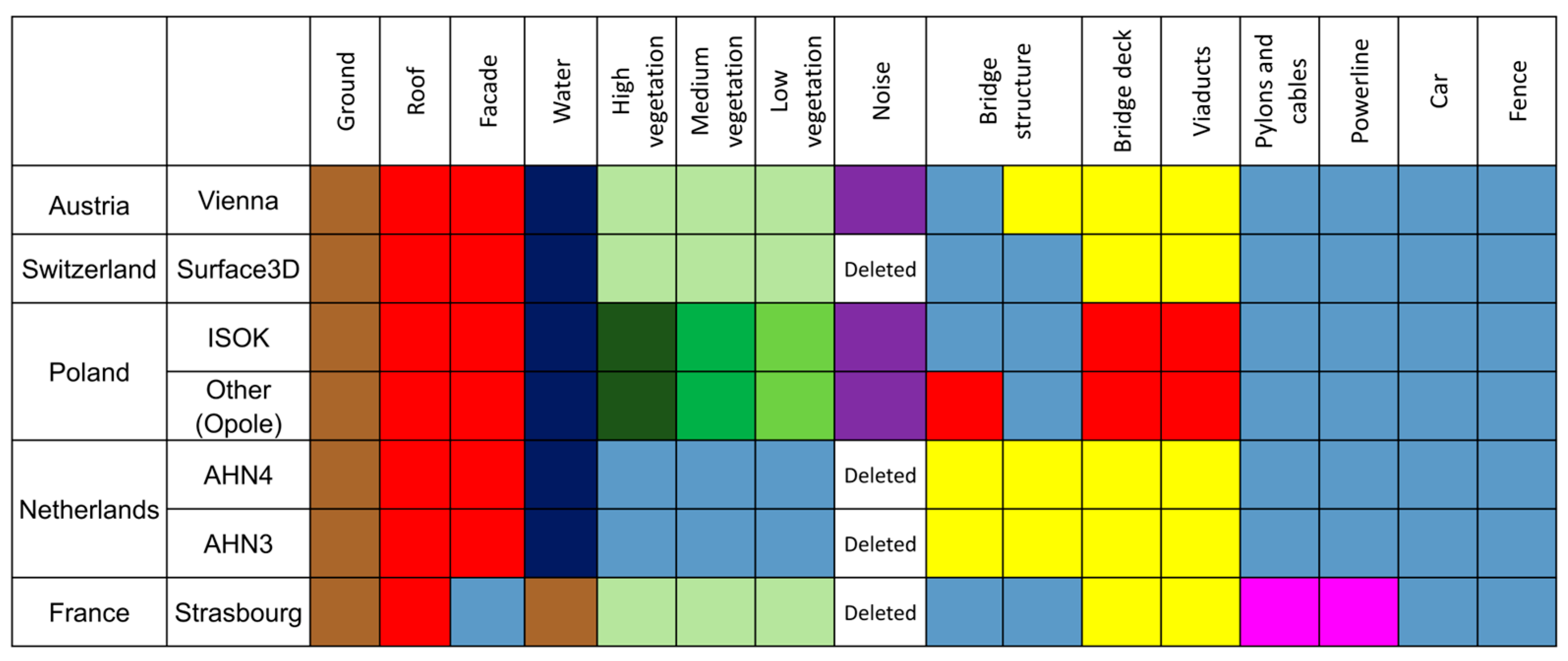
Figure 1. Classification differences between datasets. The same color indicates objects that belong to the same class in a certain dataset. Colors correspond to ASPRS definition of classes in las files: brown—ground, red—buildings, dark blue—water, green (different shades)—vegetation (high, medium, and low), yellow—bridge, pink—pylons, cables, and powerlines, purple—high and low points, and light blue—other.
Remotesensing 17 02731 g001
Figure 2. Vienna dataset: left—locations of training (red) and testing (blue) tiles; right—histogram of classes occurrences in the training dataset.
Remotesensing 17 02731 g002
Figure 3. Zurich dataset: left—locations of training (red) and testing (blue) tiles; right—histogram of classes occurrences in the training dataset.
Remotesensing 17 02731 g003
Figure 4. Opole dataset: left—locations of training (red) and testing (blue) tiles; right—histogram of classes occurrences in the training dataset.
Remotesensing 17 02731 g004
Figure 5. The summary of the usability of each dataset for evaluation of the accuracy of each class.
Remotesensing 17 02731 g005
Figure 6. Histogram of classes occurrences in Geneva, Liechtenstein, Wrocław 2011, and Wrocław 2022 datasets.
Remotesensing 17 02731 g006
Figure 7. Histogram of classes occurrences in Strasbourg, Zwolle, France, and Luxembourg datasets.
Remotesensing 17 02731 g007
Figure 8. Histogram of class occurrences in DALES, Dublin, Hessigheim, and Vaihingen datasets.
Remotesensing 17 02731 g008
Figure 9. IoU-based [%] accuracy of semantic segmentation results in Vienna data (left), Zurich data (middle), and Opole data (right) according to Experiment 1a and 1c.
Remotesensing 17 02731 g009
Figure 10. Results of semantic segmentation in Vienna data (top left), Zurich data (top right), and Opole data (bottom left) according to Experiment 1b.
Remotesensing 17 02731 g010
Figure 11. The IoU-based accuracy of semantic segmentation achieved by a classifier trained using Vienna, Opole, and Zurich training data.
Remotesensing 17 02731 g011
Figure 12. The visualization of the double ground level problem in the Dublin dataset. Top right—the top view of the tile points are colored according to the classification (brown—ground and water, red—buildings and bridges, green—vegetation, and blue—‘other’). Interest areas are marked with yellow and pink rectangles. Top left—side view of the yellow rectangle interest area. Points are colored according to the classification. Bottom left—the distance between ground levels in the yellow rectangle interest area. Points are colored according to the distance. Middle right—side view of the pink rectangle interest area. Points are colored according to the classification. Bottom right—the distance between ground levels in the pink rectangle interest area. Points are colored according to the distance.
Remotesensing 17 02731 g012
Figure 13. Luxembourg dataset colored by classification (brown—ground, red—buildings, green—vegetation, and blue—‘other’). Top left—top view at the site. The interest area is marked with a white rectangle. Top right—white interest area without ground points. Bottom right—white interest area without ‘other’ points. Bottom left—side view of the white interest area.
Remotesensing 17 02731 g013
Figure 14. Zwolle dataset colored by classification (brown—ground, red—buildings, dark blue—water, light blue—‘other’, and yellow—bridges and viaducts). Left—the top view of the area. The interest area is marked with a white rectangle. Right—zoomed in on the white interest area. Note that the vegetation is in class ‘other’.
Remotesensing 17 02731 g014
Figure 15. Strasbourg dataset colored by classification (brown—ground, red—buildings, green—vegetation, and blue—‘other’). Left—top view at the area. The interest area is marked with a white rectangle. Right—side view at the interest area. Note that building facades are in class ‘other’.
Remotesensing 17 02731 g015
Figure 16. Example of classification of infrastructure on top of a viaduct in the (a) Vienna dataset (classified as building and bridges) and (b) Zurich dataset (classified as ‘other‘); brown—ground, red—buildings and bridges, and blue—‘other’, green—vegetation.
Remotesensing 17 02731 g016
Table 1. Characteristics of all datasets used for the experiments.
# TilesTest/Train Site Area [km2]Tile Size [m]Tile
Overlap [m]
Acquisition DateAcquisition SeasonDensity [pts/m2]ClassificationType of
Dataset
Purpose
Vienna6/67.8/7.81270 × 10202010–11.2015Leaf-off23–139Ground, vegetation, buildings, water, bridge, noise, and other (5)City-wiseTrain/Test
Zurich17/1417/141000 × 100002017–2020Leaf-off (1)8–25Ground, vegetation, buildings, bridges and viaducts, water, and other (5)NationalTrain/Test
Geneva18182018–201931–57Validation
Liechtenstein24242017–201815–33Validation
Opole16/144/3.5500 × 500003.2022Leaf-off20–35Ground, high vegetation, medium vegetation, low vegetation, buildings and bridges, high points, low points, water, and other (5)City-wiseTrain/Test
Wrocław201112307.2011Leaf-on22–30NationalValidation
Wrocław202212305.2022Leaf-on22–53City-wiseValidation
Zwolle1822.51000 × 1250 (2)25 (2)2020–2022Leaf-off20–34Ground, buildings, civil structures, water, and other (5)NationalValidation
France (national point cloud)661000 × 10000--9–34Ground, low vegetation, medium vegetation, high vegetation, buildings, water, bridge, perennial soil, noise, virtual points, and otherNationalValidation
Strasbourg (point cloud acquired by city of Strasbourg)5112.75500 × 50002015–2016-17–35Ground and water, building roofs, vegetation, bridges, pylons and cables, and other (5)City-wiseValidation
Luxembourg235.75500 × 500002.2019Leaf-off21–40Ground, low vegetation, medium vegetation, high vegetation, buildings, noise, water, bridges, power lines, and otherCity-wiseValidation
DALES4010500 × 5000--48Ground, vegetation, cars, trucks, poles, power lines, fences, and buildingsBenchmarkValidation
Dublin132Irregular003.2015Leaf-off250–348HierarchicalBenchmarkValidation
Vaihingen30.13 (3)Irregular0--4Powerline, low vegetation, impervious surface, car, fence/hedge, roof, façade, shrub, and treeBenchmarkValidation
Hessigheim20.16 (3) (4)Irregular003.2016Leaf-off20Low vegetation, impervious surfaces, vehicle, urban furniture, roof, façade, shrub, tree, soil/gravel, vertical surface, and chimneyBenchmarkValidation
Summary2–510.13–24-0–252011–2022-4–348---
(1) Information based on measurement requirements stated in the documentation. (2) Not the original size provided by the mapping agency. Since the tile size provided by the agency was extremely large and hard to process, the alternative site (geotiles.nl) was used to download the data. The site preprocesses the data from mapping agencies and provides it in more convenient sizes for use in deep learning frameworks. (3) Estimated based on data. (4) Only data with available labels. (5) As presented in Figure 1.
Table 2. A summary of performed experiments for model hyperparameters adjustment. The best values for Mean and Minimum IoU are highlighted in bold.
Test NumberVoxel Size [cm]# Layers# Features for Each Layer# EpochsWeighted Loss FunctionMean IoU [%]Min. IoU [%]
Baseline871618Yes84.052.9
12571618Yes82.849.0
2851618Yes79.546.0
3891618Yes83.350.8
4871618No82.847.8
587818Yes82.849.1
6871610Yes82.949.6
7871626Yes84.152.7
Table 3. The IoU-based accuracy of the selected cross-classifiers and the joint classifier evaluated using test datasets of the same cities as training. The full results are presented in Appendix C (Table A3).
Training DatasetTesting
Dataset
Average Median IoU [%]IoU [%]
Ground and WaterVegetationBuildings and BridgesOther
MedianMeanStdMedianMeanStdMedianMeanStdMedianMeanStd
ViennaVienna84.597.397.01.894.894.23.592.488.015.753.552.213.3
OpoleVienna69.091.888.712.180.075.419.776.965.531.627.329.321.4
ZurichVienna78.295.994.85.091.690.45.689.783.117.435.737.119.4
Zurich and Opole and ViennaVienna84.997.296.92.094.994.33.393.589.810.553.850.817.2
ZurichZurich84.797.897.51.196.696.62.293.692.05.150.853.411.4
OpoleZurich76.693.593.22.792.191.73.587.681.117.833.133.011.1
ViennaZurich81.096.696.61.495.295.23.090.588.16.641.643.910.4
Zurich and Opole and ViennaZurich84.697.497.41.196.496.42.394.092.44.450.453.411.5
OpoleOpole79.996.395.91.786.986.55.191.589.65.944.748.211.7
ViennaOpole76.294.694.31.883.482.07.385.883.86.740.939.211.6
ZurichOpole76.195.194.32.382.181.48.090.987.77.836.436.613.0
Zurich and Opole and ViennaOpole82.796.696.11.986.986.65.492.590.06.554.652.410.8
Table 4. The IoU-based accuracy of the joint classifier evaluated using test datasets independent from the training data. The accuracy was evaluated using various dataset groups that are divided by horizontal lines. The top accuracy in each data group is marked with bold.
NameCountryIoU [%]
Ground and WaterVegetationBuildings and BridgesOther
MedianMeanStdMedianMeanStdMedianMeanStdMedianMeanStd
ViennaAT97.296.92.094.994.33.393.589.810.553.850.817.2
ZurichCH97.497.41.196.496.42.394.092.44.450.453.411.5
OpolePL96.696.11.986.986.65.492.590.06.554.652.410.8
GenevaCH96.796.81.095.995.41.691.887.110.352.751.99.8
LichtensteinLI95.995.71.695.494.43.392.291.63.034.036.77.9
Wrocław 2011PL92.293.42.777.378.68.491.987.112.013.517.811.9
Wrocław 2022PL94.293.13.290.490.24.093.289.97.041.039.313.8
ZwolleNL97.397.12.190.886.710.4
FranceFR94.490.77.990.785.017.077.666.432.029.523.018.4
StrasbourgFR92.491.53.882.779.015.6
LuxembourgLU91.090.53.7
DublinIE75.572.619.119.620.011.9
DALESUSA95.394.72.389.589.23.594.891.314.347.846.39.2
VaihingenDE90.089.62.768.070.44.391.891.21.422.723.43.2
HessigheimDE91.691.63.079.579.53.991.391.32.731.431.41.1
Table 5. The F1 score results achieved for the Vaihingen dataset and described in selected literature.
Imperv. SurfLow Veg.ShrubTreeRoofFacadeCarFence/HedgePowerline
[18]90.281.783.895.047.4-
[12]91.577.945.982.594.049.373.418.037.5
[11]91.682.049.682.694.461.577.844.275.4
[44]91.482.744.279.892.456.876.939.677.0
[45]91.280.843.883.693.158.662.153.755.7
[46]90.580.048.375.792.757.978.545.575.5
[47]99.386.539.472.691.144.275.219.568.1
[48]91.182.046.883.193.660.876.540.556.1
[50]91.982.650.782.794.559.374.939.963.0
[52]90.280.534.774.593.147.345.77.670.1
Table 6. The F1 score results achieved for the Hessigheim dataset as presented on the competition website.
MethodGravelImperv. SurfacesLow Veg.ShrubTreeRoofFacadeChimneyVehicleUrban fur.Vert. Surf.
Zhan58.487.589.465.293.896.869.375.467.545.753.8
X51.787.589.366.493.696.068.376.266.740.554.7
Ifp-RF55.585.987.559.892.496.064.156.557.039.134.5
Disclaimer/Publisher’s Note: The statements, opinions and data contained in all publications are solely those of the individual author(s) and contributor(s) and not of MDPI and/or the editor(s). MDPI and/or the editor(s) disclaim responsibility for any injury to people or property resulting from any ideas, methods, instructions or products referred to in the content.