
An Adaptive CNN-Based Approach for Improving SWOT-Derived Sea-Level Observations Using Drifter Velocities


Abstract
1. Introduction
2. Datasets
2.1. SWOT Sea-Surface Height Anomalies
2.2. DUACS Altimetry Data
2.3. Drifter Velocity Observations
2.4. Surface Wind Data
2.5. SWOT Level-3 Product
3. SWOT SSHA Filtering Methodology
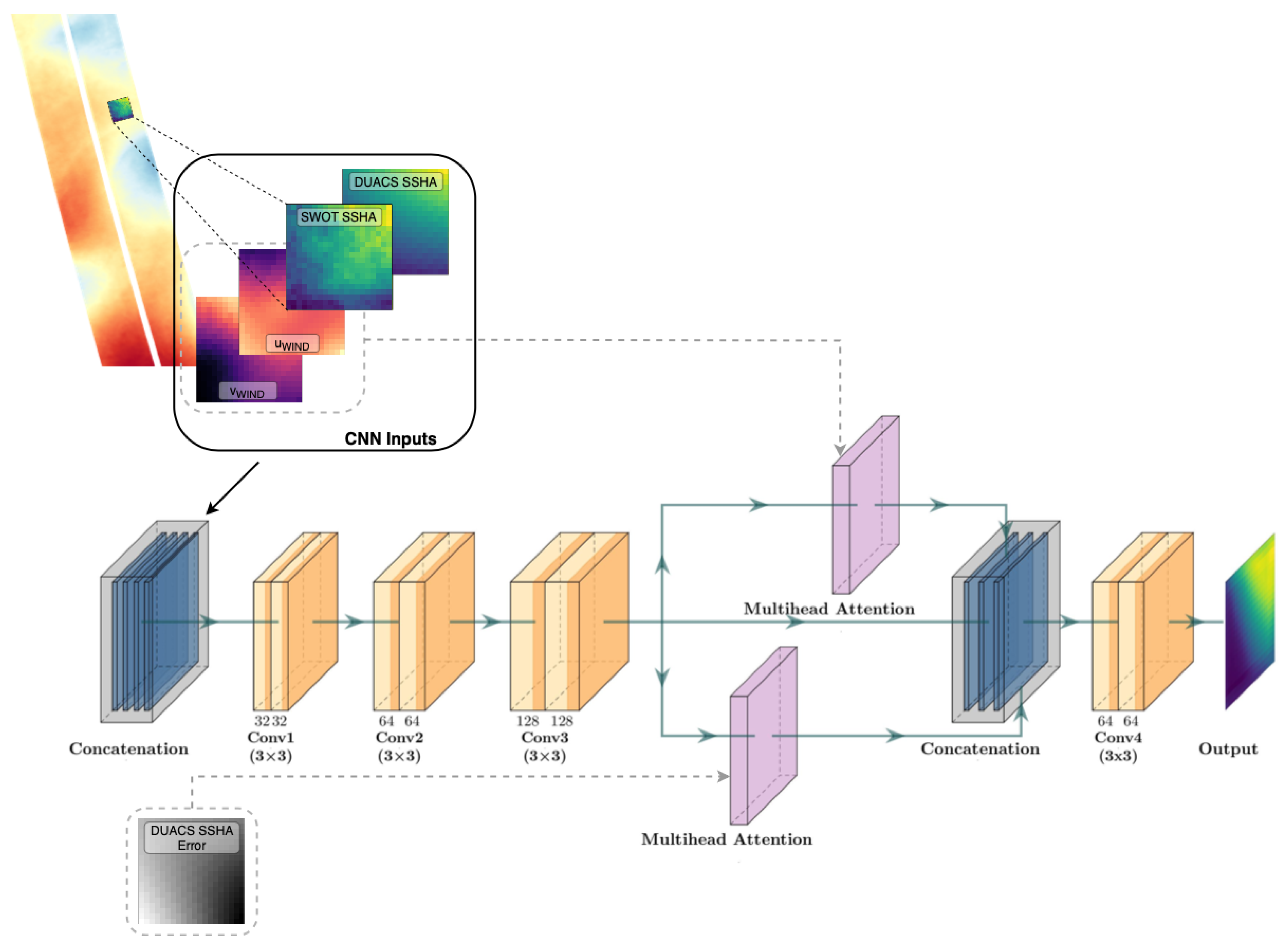
3.1. Convolutional Neural Network Architecture
3.2. The Custom Loss Function
3.3. Data Preparation
- Matchup Database:
- The preparation of the data required for the CNN training involves creating a matchup database that pairs tiles from SWOT datasets, drifter velocities, DUACS SSHA and SSHA error, and wind data for the same date. The matchup covers the period July 2023–April 2024. A tile size of 20 × 20 pixels (corresponding to 40 × 40 km, given the 2 × 2 km resolution of the SWOT Expert product) was selected as a trade-off between computational efficiency and the need to capture mesoscale features within the SWOT swath. This size also allows the tiles to be fully contained within the SWOT swath (69 pixels wide), avoiding edge effects and preserving spatial context. The objective is to select 20 × 20 pixel tiles around specific drifter positions, ensuring that the tiles’ edges are positioned at least 5 pixels away from the image borders to reduce spurious edge effects during the training and allow for an accurate estimation of SSHA gradients. For each drifter location, 20 tiles have been selected randomly among all possible tiles, including the drifter locations. This strategy allowed us to generate diverse samples of SWOT data from a single drifter matchup. It served as an augmentation strategy to improve the network ability to associate the most relevant spatial features detected over the relatively small tiles that are positioned differently around the drifter matchup. Once these tiles have been identified, the corresponding 20 × 20 pixel tiles from the other datasets (SWOT_L3, DUACS SSHA, DUACS SSHA error and wind data) were extracted for the same spatial area and date, ensuring consistency across all variables. This procedure resulted in a total of 18634 matchup samples, which thus lead to 372,680 tiles available for network training. This approach was chosen to enhance memory efficiency and processing speed, as working with smaller tiles reduces computational demands, but also considering the small swath of original SWOT observations. By selecting 20 tiles per matchup, our aim was to expose the model to a wide range of oceanographic features within the dataset, allowing it to learn from the diversity of patterns present.
- Inputs Pre-processing:
- Before training the CNN, we preprocess the input data to ensure consistency and improve the model’s learning ability. First, we exclude the equatorial band (10°S – 10°N), where geostrophic balance does not hold, and we discard suspect high-velocity drifter points by selecting only locations where < 2 . Next, we remove the mean SSHA from each 20 × 20 pixel tile of the DUACS fields to eliminate large-scale biases and regional offsets. For SWOT SSHA, instead of subtracting the tile mean, we apply a large-scale spatial smoothing using a moving average filter with a 30 × 30 kernel. This is implemented using the convolve function from the Astropy 6.0 library in Python 3.11, which acts as a low-pass filter by averaging the SSHA values within a 30 × 30 neighborhood around each pixel. We then subtract this smoothed field from the original SWOT SSHA. This operation isolates mesoscale and smaller-scale features by removing low-frequency variability, allowing the model to focus on resolving local structures and high-frequency variations. Finally, we apply min–max normalization to all input variables to standardize their range and improve model convergence:where X is the original (non-normalized) variable, and are the minimum and maximum values of X, respectively, and is the normalized variable.This normalization scales each variable to the range [0, 1], ensuring that different inputs contribute proportionally during training and preventing numerical instabilities. After training the model, the predicted anomalies are denormalized and the large-scale background—previously removed using the smoothing filter—is summed to reconstruct the full SSHA fields. The dataset is split into 80% for training and 20% for testing, with 15% of the training dataset reserved for validation. This split ensures sufficient data for model optimization while maintaining an independent test set for performance evaluation. The split is applied at the block level, where each block consists of the 20 tiles associated with the same drifter observation. To ensure an unbiased and independent separation, the blocks are randomly assigned to one of the three subsets (training, validation, or testing), ensuring that all tiles corresponding to a single drifter position are assigned to only one subset. This approach prevents model overfitting by avoiding the use of data from the same drifter trajectory across multiple datasets, and further ensures that no duplicate data appears in different subsets.
3.4. Training and Optimization
3.5. Evaluation Metrics
3.6. Reconstruction of the SWOT Track
3.7. Filtering Methods for Comparison
4. Results
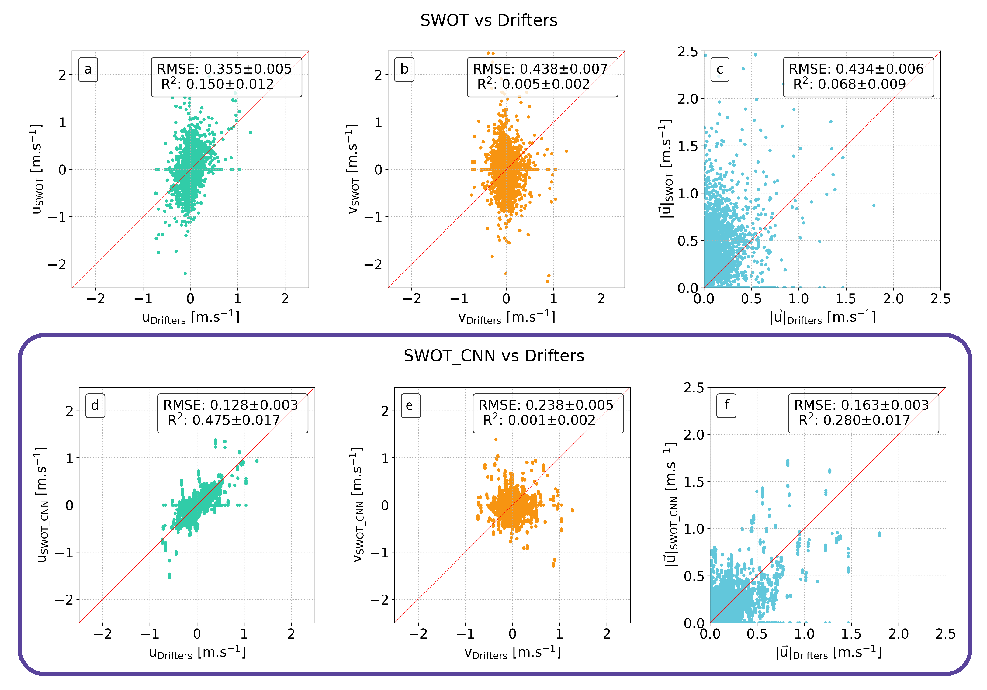
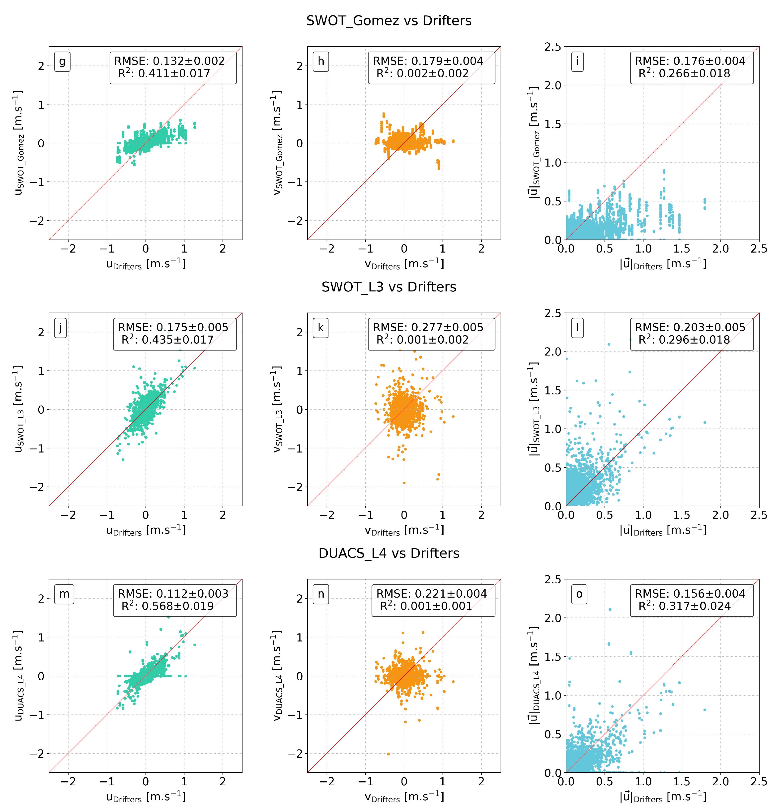
4.1. Evaluation of Geostrophic Velocity
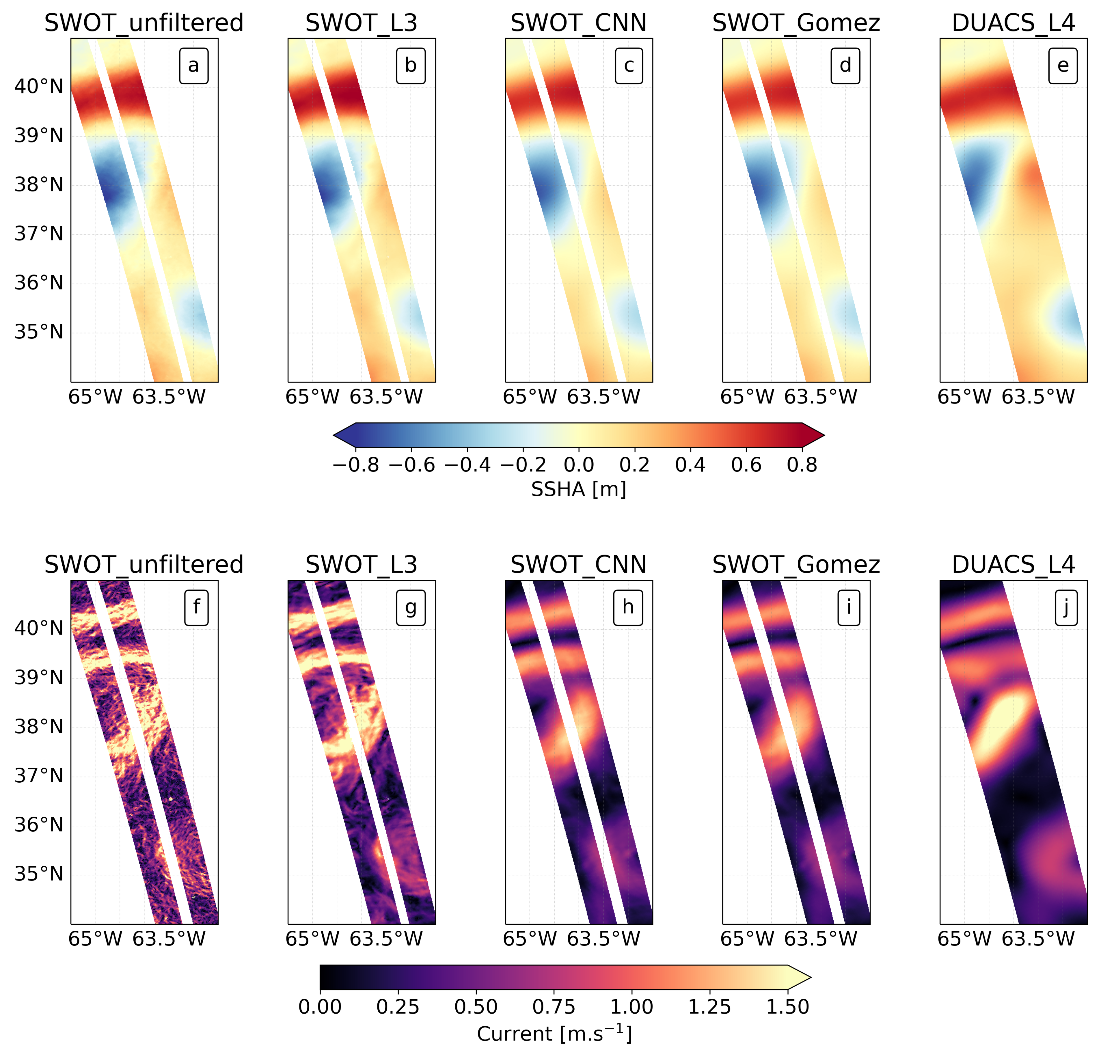
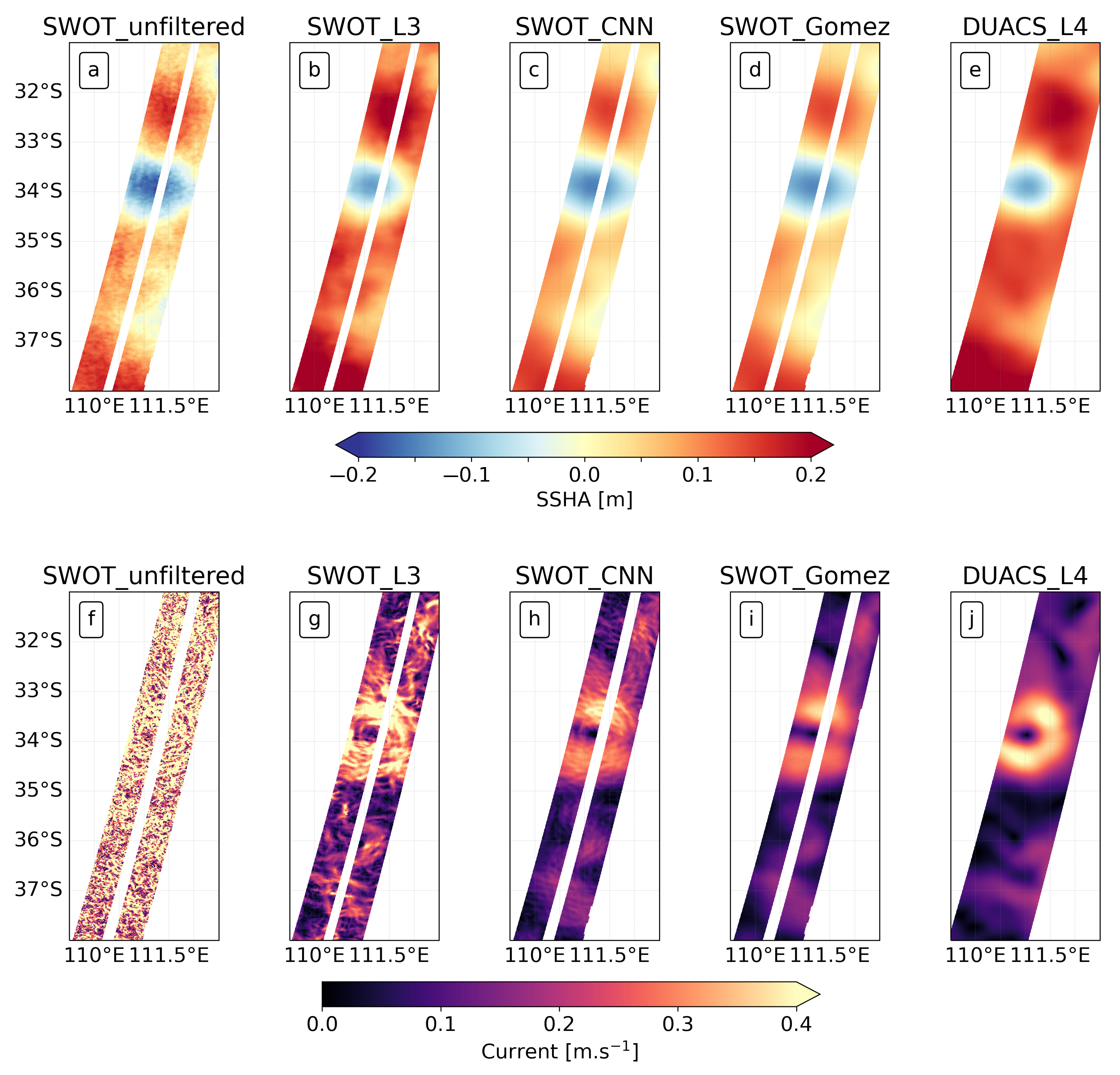
4.2. Reconstructed Track
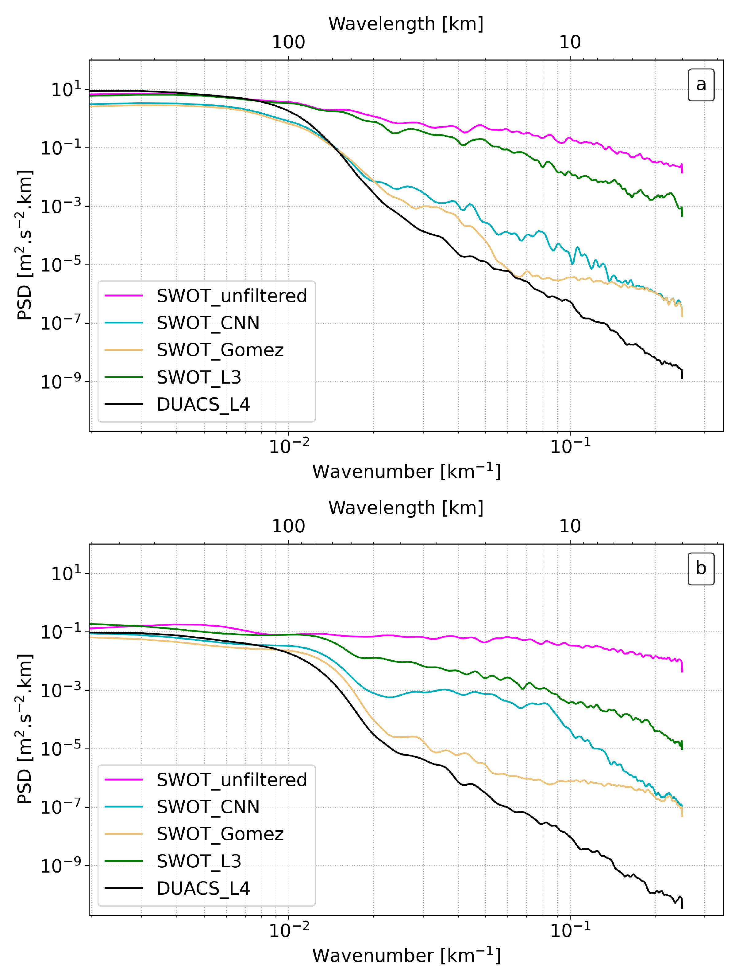
4.3. Spectral Analysis
5. Discussion/Conclusions
Author Contributions
Funding
Data Availability Statement
Acknowledgments
Conflicts of Interest
Abbreviations
| ADT | Absolute Dynamic Topography |
| CMEMS | Copernicus Marine Environment Monitoring Service |
| CNN | Convolutional Neural Network |
| DUACS | Data Unification and Altimeter Combination System |
| KaRIn | Ka-band Radar Interferometer |
| KE | Kinetic Energy |
| MSE | Mean Square Error |
| PSD | Power Spectral Density |
| RMSE | Root Mean Square Error |
| SSH | Sea-Surface Height |
| SSHA | Sea-Surface Height Anomaly |
| SWOT | Surface Water and Ocean Topography |
References
- Fu, L.L.; Cazenave, A. Satellite Altimetry and Earth Sciences: A Handbook of Techniques and Applications; Elsevier: Amsterdam, The Netherlands, 2000; Volume 69. [Google Scholar]
- Morrow, R.; Fu, L.L.; Farrar, J.T.; Seo, H.; Traon, P.Y.L. Ocean Eddies and Mesoscale Variability. In Satellite Altimetry over Oceans and Land Surfaces; CRC Press: Boca Raton, FL, USA, 2017; pp. 315–342. [Google Scholar] [CrossRef]
- Fu, L.L.; Alsdorf, D.; Rodriguez, E.; Morrow, R.; Mognard, N.; Lambin, J.; Vaze, P.; Lafon, T. The SWOT (Surface Water and Ocean Topography) Mission: Spaceborne Radar Interferometry for Oceanographic and Hydrological Applications. In Proceedings of the OCEANOBS’09 Conference, Venice, Italy, 21–25 September 2009. [Google Scholar]
- Fu, L.L.; Ubelmann, C. On the Transition from Profile Altimeter to Swath Altimeter for Observing Global Ocean Surface Topography. J. Atmos. Ocean. Technol. 2014, 31, 560–568. [Google Scholar] [CrossRef]
- Morrow, R.; Fu, L.L.; Ardhuin, F.; Benkiran, M.; Chapron, B.; Cosme, E.; D’Ovidio, F.; Farrar, J.T.; Gille, S.T.; Lapeyre, G.; et al. Global observations of fine-scale ocean surface topography with the Surface Water and Ocean Topography (SWOT) Mission. Front. Mar. Sci. 2019, 6, 433647. [Google Scholar] [CrossRef]
- Du, T.; Jing, Z. Fine-Scale Eddies Detected by SWOT in the Kuroshio Extension. Remote Sens. 2024, 16, 3488. [Google Scholar] [CrossRef]
- Zhang, H.; Fan, C.; Sun, L.; Meng, J. Study of the ability of SWOT to detect sea surface height changes caused by internal solitary waves. Acta Oceanol. Sin. 2024, 43, 54–64. [Google Scholar] [CrossRef]
- Zhang, Z.; Miao, M.; Qiu, B.; Tian, J.; Jing, Z.; Chen, G.; Chen, Z.; Zhao, W. Submesoscale Eddies Detected by SWOT and Moored Observations in the Northwestern Pacific. Geophys. Res. Lett. 2024, 51, e2024GL110000. [Google Scholar] [CrossRef]
- Chelton, D.B.; Samelson, R.M.; Farrar, J.T. The Effects of Uncorrelated Measurement Noise on SWOT Estimates of Sea Surface Height, Velocity, and Vorticity. J. Atmos. Ocean. Technol. 2022, 39, 1053–1083. [Google Scholar] [CrossRef]
- Fan, L.; Zhang, F.; Fan, H.; Zhang, C. Brief review of image denoising techniques. Vis. Comput. Ind. Biomed. Art 2019, 2, 7. [Google Scholar] [CrossRef]
- Ubelmann, C.; Dibarboure, G.; Dubois, P. A Cross-Spectral Approach to Measure the Error Budget of the SWOT Altimetry Mission over the Ocean. J. Atmos. Ocean. Technol. 2018, 35, 845–857. [Google Scholar] [CrossRef]
- Metref, S.; Cosme, E.; Sommer, J.L.; Poel, N.; Brankart, J.M.; Verron, J.; Navarro, L.G. Reduction of Spatially Structured Errors in Wide-Swath Altimetric Satellite Data Using Data Assimilation. Remote Sens. 2019, 11, 1336. [Google Scholar] [CrossRef]
- Gómez-Navarro, L.; Cosme, E.; Sommer, J.L.; Papadakis, N.; Pascual, A. Development of an Image De-Noising Method in Preparation for the Surface Water and Ocean Topography Satellite Mission. Remote Sens. 2020, 12, 734. [Google Scholar] [CrossRef]
- Tréboutte, A.; Carli, E.; Ballarotta, M.; Carpentier, B.; Faugère, Y.; Dibarboure, G. KaRIn Noise Reduction Using a Convolutional Neural Network for the SWOT Ocean Products. Remote Sens. 2023, 15, 2183. [Google Scholar] [CrossRef]
- Zhao, Q.; Peng, S.; Wang, J.; Li, S.; Hou, Z.; Zhong, G. Applications of deep learning in physical oceanography: A comprehensive review. Front. Mar. Sci. 2024, 11, 1396322. [Google Scholar] [CrossRef]
- Dibarboure, G.; Anadon, C.; Briol, F.; Cadier, E.; Chevrier, R.; Delepoulle, A.; Faugère, Y.; Laloue, A.; Morrow, R.; Picot, N.; et al. Blending 2D topography images from the Surface Water and Ocean Topography (SWOT) mission into the altimeter constellation with the Level-3 multi-mission Data Unification and Altimeter Combination System (DUACS). Ocean Sci. 2025, 21, 283–323. [Google Scholar] [CrossRef]
- AVISO+. SSALTO/DUACS User Handbook: MSLA and (M)ADT Near-Real Time and Delayed Time Products (CLS-DOS-NT-06-034); CLS: Toulouse, France, 2016. [Google Scholar]
- JPL D-56407. SWOT Product Description Document: Level 2 KaRIn Low Rate Sea Surface Height (L2_LR_SSH) Data Product (Internal Document); Revision C. Jet Propulsion Laboratory: Pasadena, CA, USA, 2024. [Google Scholar]
- JPL D-109532. SWOT Science Data Products User Handbook (Internal Document); Revision A; Jet Propulsion Laboratory: Pasadena, CA, USA, 2024. [Google Scholar]
- Mulet, S.; Rio, M.H.; Etienne, H.; Artana, C.; Cancet, M.; Dibarboure, G.; Feng, H.; Husson, R.; Picot, N.; Provost, C.; et al. The new CNES-CLS18 global mean dynamic topography. Ocean Sci. 2021, 17, 789–808. [Google Scholar] [CrossRef]
- Lumpkin, R.; Özgökmen, T.; Centurioni, L. Advances in the Application of Surface Drifters. Annu. Rev. Mar. Sci. 2017, 9, 59–81. [Google Scholar] [CrossRef]
- Buongiorno Nardelli, B.; Mulet, S.; Iudicone, D. Three-Dimensional Ageostrophic Motion and Water Mass Subduction in the Southern Ocean. J. Geophys. Res. Ocean. 2018, 123, 1533–1562. [Google Scholar] [CrossRef]
- Pielawski, N.; Wählby, C. Introducing Hann windows for reducing edge-effects in patch-based image segmentation. PLoS ONE 2019, 15, e0229839. [Google Scholar] [CrossRef]
- Le Traon, P.Y.; Klein, P.; Hua, B.L.; Dibarboure, G. Do Altimeter Wavenumber Spectra Agree with the Interior or Surface Quasigeostrophic Theory? J. Phys. Oceanogr. 2008, 38, 1137–1142. [Google Scholar] [CrossRef]
- Ballarotta, M.; Ubelmann, C.; Pujol, M.I.; Taburet, G.; Fournier, F.; Legeais, J.F.; Faugère, Y.; Delepoulle, A.; Chelton, D.; Dibarboure, G.; et al. On the resolutions of ocean altimetry maps. Ocean Sci. 2019, 15, 1091–1109. [Google Scholar] [CrossRef]
- Ciani, D.; Rio, M.H.; Buongiorno Nardelli, B.; Etienne, H.; Santoleri, R. Improving the Altimeter-Derived Surface Currents Using Sea Surface Temperature (SST) Data: A Sensitivity Study to SST Products. Remote Sens. 2020, 12, 1601. [Google Scholar] [CrossRef]
- Fablet, R.; Febvre, Q.; Chapron, B. Multimodal 4DVarNets for the Reconstruction of Sea Surface Dynamics From SST-SSH Synergies. IEEE Trans. Geosci. Remote Sens. 2023, 61, 4204214. [Google Scholar] [CrossRef]
- Ciani, D.; Asdar, S.; Buongiorno Nardelli, B. Improved Surface Currents from Altimeter-Derived and Sea Surface Temperature Observations: Application to the North Atlantic Ocean. Remote Sens. 2024, 16, 640. [Google Scholar] [CrossRef]

| SWOT_Unfiltered | SWOT_CNN | SWOT_Gómez | SWOT_L3 | DUACS_L4 | |
|---|---|---|---|---|---|
| 0.355 ± 0.005 | 0.128 ± 0.003 | 0.132 ± 0.002 | 0.175 ± 0.005 | 0.112 ± 0.003 | |
| 0.438 ± 0.007 | 0.238 ± 0.005 | 0.179 ± 0.004 | 0.277 ± 0.005 | 0.221 ± 0.004 | |
| 0.434 ± 0.006 | 0.163 ± 0.003 | 0.176 ± 0.004 | 0.203 ± 0.005 | 0.156 ± 0.004 | |
| 0.150 ± 0.012 | 0.475 ± 0.017 | 0.411 ± 0.017 | 0.435 ± 0.017 | 0.568 ± 0.017 | |
| 0.005 ± 0.002 | 0.001 ± 0.002 | 0.002 ± 0.002 | 0.001 ± 0.002 | 0.001 ± 0.001 | |
| 0.4068 ± 0.009 | 0.280 ± 0.017 | 0.266 ± 0.018 | 0.296 ± 0.018 | 0.317 ± 0.024 | |
| Spectral Noise Reduction | - | 87.0% | 89.6% | 58.5% | - |
Disclaimer/Publisher’s Note: The statements, opinions and data contained in all publications are solely those of the individual author(s) and contributor(s) and not of MDPI and/or the editor(s). MDPI and/or the editor(s) disclaim responsibility for any injury to people or property resulting from any ideas, methods, instructions or products referred to in the content. |
© 2025 by the authors. Licensee MDPI, Basel, Switzerland. This article is an open access article distributed under the terms and conditions of the Creative Commons Attribution (CC BY) license (https://creativecommons.org/licenses/by/4.0/).
Share and Cite
Asdar, S.; Buongiorno Nardelli, B. An Adaptive CNN-Based Approach for Improving SWOT-Derived Sea-Level Observations Using Drifter Velocities. Remote Sens. 2025, 17, 2681. https://doi.org/10.3390/rs17152681
Asdar S, Buongiorno Nardelli B. An Adaptive CNN-Based Approach for Improving SWOT-Derived Sea-Level Observations Using Drifter Velocities. Remote Sensing. 2025; 17(15):2681. https://doi.org/10.3390/rs17152681
Chicago/Turabian StyleAsdar, Sarah, and Bruno Buongiorno Nardelli. 2025. "An Adaptive CNN-Based Approach for Improving SWOT-Derived Sea-Level Observations Using Drifter Velocities" Remote Sensing 17, no. 15: 2681. https://doi.org/10.3390/rs17152681
APA StyleAsdar, S., & Buongiorno Nardelli, B. (2025). An Adaptive CNN-Based Approach for Improving SWOT-Derived Sea-Level Observations Using Drifter Velocities. Remote Sensing, 17(15), 2681. https://doi.org/10.3390/rs17152681