Article

Robust Adaptive Multiple Backtracking VBKF for In-Motion Alignment of Low-Cost SINS/GNSS

1
School of Automation, Jiangsu University of Science and Technology, Zhenjiang 212100, China
2
Ocean College, Zhejiang University, Zhoushan 316021, China
3
Shanghai Astronomical Observatory, Chinese Academy of Sciences, Shanghai 200030, China
4
School of Surveying and Land Information Engineering, Henan Polytechnic University, Jiaozuo 454003, China
5
School of Resources and Environmental Science and Engineering, Hubei University of Science and Technology, Xianning 437100, China
6
Research Center of Beidou + Industrial Development of Key Research Institute of Humanities and Social Sciences of Hubei Province, Hubei University of Science and Technology, Xianning 437100, China
7
School of Civil and Environmental Engineering, University of New South Wales, Sydney, NSW 2052, Australia
*
Author to whom correspondence should be addressed.
Remote Sens. 2025, 17(15), 2680; https://doi.org/10.3390/rs17152680
Submission received: 6 June 2025 / Revised: 28 July 2025 / Accepted: 31 July 2025 / Published: 2 August 2025
(This article belongs to the Section Urban Remote Sensing)

Abstract

The low-cost Strapdown Inertial Navigation System (SINS)/Global Navigation Satellite System (GNSS) is widely used in autonomous vehicles for positioning and navigation. Initial alignment is a critical stage for SINS operations, and the alignment time and accuracy directly affect the SINS navigation performance. To address the issue that low-cost SINS/GNSS cannot effectively achieve rapid and high-accuracy alignment in complex environments that contain noise and external interference, an adaptive multiple backtracking robust alignment method is proposed. The sliding window that constructs observation and reference vectors is established, which effectively avoids the accumulation of sensor errors during the full integration process. A new observation vector based on the magnitude matching is then constructed to effectively reduce the effect of outliers on the alignment process. An adaptive multiple backtracking method is designed in which the window size can be dynamically adjusted based on the innovation gradient; thus, the alignment time can be significantly shortened. Furthermore, the modified variational Bayesian Kalman filter (VBKF) that accurately adjusts the measurement noise covariance matrix is proposed, and the Expectation–Maximization (EM) algorithm is employed to refine the prior parameter of the predicted error covariance matrix. Simulation and experimental results demonstrate that the proposed method significantly reduces alignment time and improves alignment accuracy. Taking heading error as the critical evaluation indicator, the proposed method achieves rapid alignment within 120 s and maintains a stable error below 1.2° after 80 s, yielding an improvement of over 63% compared to the backtracking-based Kalman filter (BKF) method and over 57% compared to the fuzzy adaptive KF (FAKF) method.

1. Introduction

The Strapdown Inertial Navigation System (SINS), with its all-weather autonomy and ability to provide attitude, velocity, and position information, offers key advantages for independent navigation [1,2,3,4]. Owing to these features, it has been widely applied in autonomous driving, autonomous underwater vehicles (AUVs), unmanned aerial vehicles, Internet of Things (IoT), and smart cities [5]. SINS calculates the vehicle’s attitude, velocity, and position by processing raw inertial sensor measurements [6]. Initial alignment is critical for subsequent navigation performance as it determines the carrier’s initial attitude accuracy [7,8,9,10,11]. Initial alignment can be divided into two basic types based on the carrier’s motion state: static alignment and in-motion alignment [12]. However, because static alignment becomes ineffective in dynamic environments, in-motion alignment methods have been proposed to enable real-time alignment during continuous maneuvers [13,14,15,16].
To address the requirements of in-motion alignment, Wu et al. [17] proposed an Optimization-Based Alignment (OBA) method that transforms the attitude determination problem into a Wahba problem to make full use of observation vectors. Based on this work, Wu et al. [18] proposed a GPS-aided coarse alignment method based on velocity vector integration, which suppresses random noise in the alignment process to a certain extent. However, when the GPS-aided information contains a large number of outliers, such as in complex urban environments where tall buildings are densely distributed, forests are obscured, and there are tunnels or elevated bridges, the performance of the above-mentioned methods is severely limited. In [5], a Doppler velocity log (DVL)-aided in-motion alignment method based on Huber’s robust theory was designed to reduce the effect of outliers. Xu et al. [19] proposed a robust attitude determination method to accomplish the in-motion alignment process when GPS output contains outliers. However, these methods are only applicable to high-accuracy SINS, and the outlier isolation method for low-cost SINS remains to be studied.
To shorten the time of in-motion alignment, researchers have proposed backtracking alignment methods that artificially extend navigation data, achieving rapid convergence of alignment results [20,21,22,23]. Chang et al. [24] proposed a fast initial alignment method based on a backtracking integration procedure, which can reuse the inertial measurement unit (IMU) and GPS information. Fu et al. [25] proposed a backtracking-based alignment method that reuses stored sensor data for navigation updates and Kalman filtering in the geographic frame, which simplifies the algorithm and improves alignment accuracy. However, the standard backtracking method may not be able to fully utilize the information in the navigation data in complex environments. To improve the utilization of navigation data, Lin et al. [26] proposed a high-accuracy backtracking alignment method that estimates and compensates for transient acceleration errors. Wei et al. [27] proposed an improved alignment method based on backtracking navigation, which fully considered the low-cost inertial sensor biases and corrected the correlated errors to make full use of the limited observation information. However, the aforementioned methods do not consider that the outdated historical data may no longer reflect current noise characteristics, thereby degrading the subsequent estimation performance [28,29,30].
Furthermore, to accomplish in-motion alignment, it is essential to develop novel filtering methods to accurately estimate the sensor biases and correlated errors. Existing alignment methods usually estimate unknown parameters by using the Kalman filter (KF), which assumes that the sensor noise follows a Gaussian distribution [31,32,33,34,35,36]. However, affected by outlier interference, the noise distribution of measured values provided by the sensors is often non-Gaussian noise. In order to improve the performance of the filter, Meng et al. [37] proposed a dual-input interval type-2 fuzzy inference system that allows for real-time adjustments of the measurement noise covariance matrix using fuzzy adjustment strategies. Shi et al. [38] proposed an adaptive Kalman filter to suppress the adverse effects of outliers and approximate the unknown measurement noise covariance matrix using the variational Bayesian (VB) method. Huang et al. [39] proposed a novel VB Kalman filter to address deviations from Gaussian noise distributions, which estimates the varying measurement noise covariance matrix by manually selecting prior parameters. However, the manual selection of prior parameters may be inaccurate in some cases, and the severe maneuvers of vehicles can cause the sensor noise to exhibit heavy-tailed characteristics in complex environments, which leads to a significant decline in the performance of the filters.
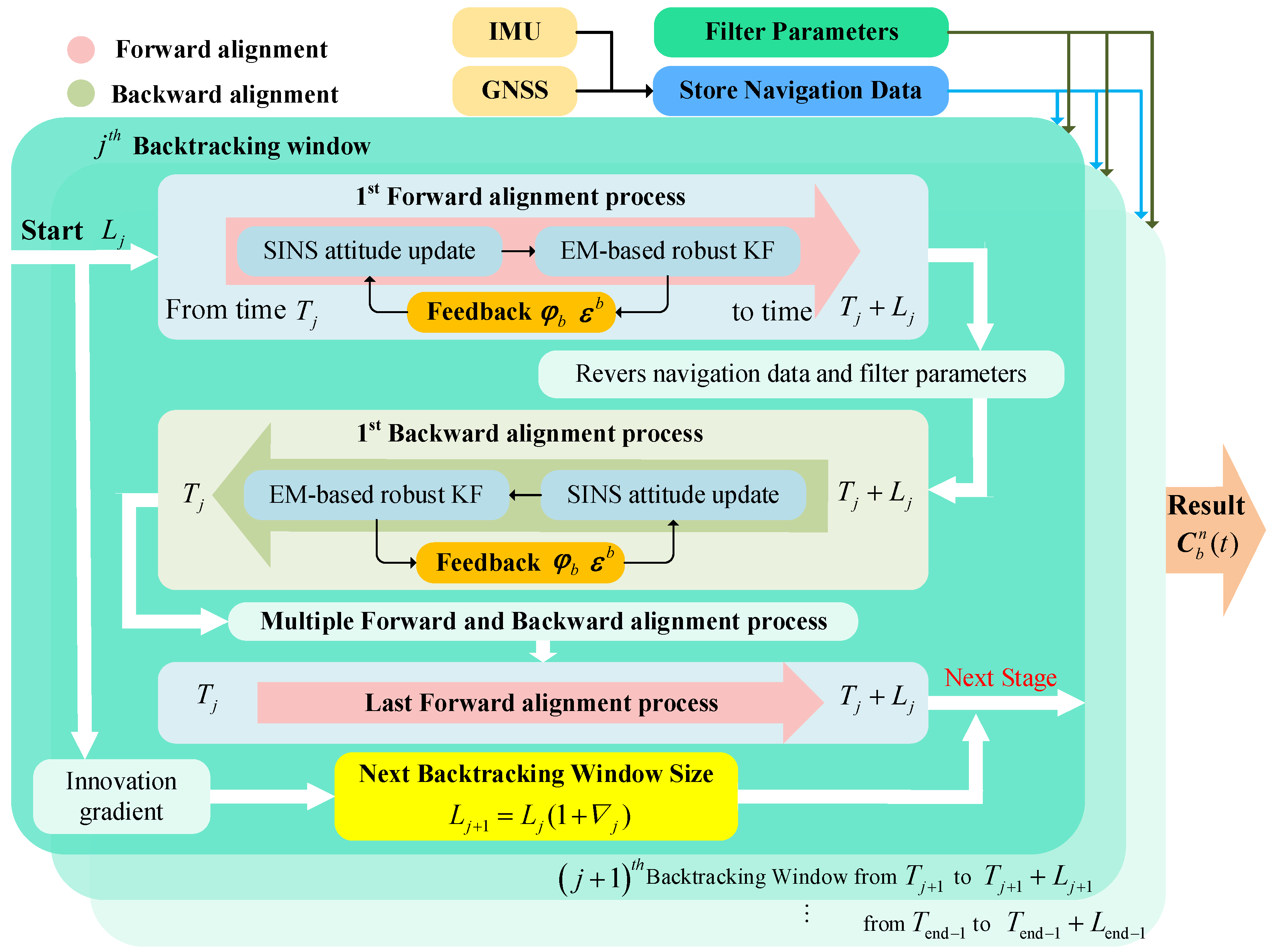
To address the above problems, this paper proposes a novel adaptive multiple backtracking robust in-motion alignment method. The calculation flow of the proposed method is illustrated in Figure 1. Specifically, a linear state-space model is established, incorporating GNSS-aided information to estimate gyroscope constant biases and the equivalent rotation vector between the true and calculated body frames. By reconstructing the observation vector using residual information, outlier detection and isolation within the GNSS-aided data are performed. To shorten the alignment time, a multiple backtracking strategy combined with an adaptive window adjustment approach is developed to make full use of the navigation data and mitigate the effect of noise with varying statistical characteristics. An Expectation–Maximization-based robust Kalman filter is employed to address situations where system noise deviates from the Gaussian distribution, thereby improving the estimation accuracy of the measurement noise covariance matrix. The main contributions of this paper are as follows:
  • Observation and reference vectors are constructed using the sliding window method to mitigate the accumulation of sensor errors. A weighting function is designed using a magnitude matching method to reconstruct the observation vector, enabling the detection and isolation of outliers.
  • An adaptive window adjustment multiple backtracking approach is proposed to effectively utilize navigation data and significantly shorten alignment time in complex environments. This approach intelligently determines the size of the backtracking window based on an innovation gradient, which effectively improves alignment accuracy.
  • An EM-based robust variational Bayesian Kalman filter is designed to accurately estimate the alignment errors in complex interference environments. Within the proposed technique, the EM and VB methods are employed to estimate the inaccurate predicted error and measurement noise covariance matrices, respectively.
The remainder of this paper is organized as follows. Section 2 describes an in-motion alignment model for the SINS that suppresses the interference of outliers. Section 3 illustrates the adaptive multiple backtracking EM-based robust variational Bayesian Kalman filter scheme in detail. Section 4 compares the alignment performance of the proposed method with those of the existing typical methods through simulations and field tests. Finally, conclusions are drawn in Section 5. The important symbols used throughout the study are summarized in Table 1.

2. In-Motion Alignment Model

2.1. Traditional In-Motion Alignment Method

According to the chain rule for attitude matrices, the time-varying attitude matrix C b n ( t ) can be decomposed into the product of three attitude matrices, and it can be written as follows:
C b n ( t ) = C n ( t ) n ( 0 ) T C b ( 0 ) n ( 0 ) C b ( t ) b ( 0 )
where C n ( t ) n ( 0 ) represents the attitude matrix of the navigation frame from the current time to the initial time. C b ( t ) b ( 0 ) represents the attitude matrix of the body frame from the current time to the initial time. C b ( 0 ) n ( 0 ) is the constant attitude matrix that transforms from the initial body frame to the initial navigation frame.
The two time-varying attitude matrices C n ( t ) n ( 0 ) and C b ( t ) b ( 0 ) in (1) can be obtained by integrating the following differential equations:
C ˙ n ( t ) n ( 0 ) = C n ( t ) n ( 0 ) ω i n n ( t ) ×
C ˙ b ( t ) b ( 0 ) = C b ( t ) b ( 0 ) ω i b b ( t ) ×
where ω i n n ( t ) is determined based on the carrier’s current geographic location, ω i b b ( t ) is obtained from the gyroscope output, and ( ) × represents the corresponding vector’s skew-symmetric matrix form.
The constant attitude matrix C b ( 0 ) n ( 0 ) is obtained by appropriately manipulating the specific-force equation, thereby transforming the attitude determination problem into a Wahba problem. Solving the Wahba problem subsequently yields the optimal estimation of this matrix. The specific-force equation is expressed as
V ˙ n = C n ( 0 ) n ( t ) C b ( 0 ) n ( 0 ) C b ( t ) b ( 0 ) f b 2 ω i e n + ω e n n × V n + g n
By integrating both sides of (4) and performing the necessary rearrangements, the relationship can be expressed in terms of the reference vector α ν and the observation vector β ν as follows:
β ν = C b ( 0 ) n ( 0 ) α ν
where
α ν = 0 t C b ( t ) b ( 0 ) f b d t β ν = 0 t C n ( t ) n ( 0 ) V ˙ n d t + 0 t C n ( t ) n ( 0 ) ( 2 ω i e n + ω e n n ) × V n d t 0 t C n ( t ) n ( 0 ) g n d t
At this stage, the determination of C b ( 0 ) n ( 0 ) is reformulated as a Wahba problem. The corresponding performance metric W * is defined as follows:
W * = 1 2 i = 1 k β C b ( 0 ) n ( 0 ) α 2
In (7), the optimal constant attitude matrix C b ( 0 ) n ( 0 ) is obtained by solving this problem via the Singular Value Decomposition (SVD) method.
However, the traditional alignment methods described above employ full-integration formulations, causing sensor errors to accumulate continuously from the initial epoch and thereby reducing alignment accuracy. Outliers in the GNSS measurements further reduce the accuracy of β ν and may even cause the failure of the alignment process. Given the limitations of traditional methods, exploring new outlier isolation approaches is essential.

2.2. Outliers’ Isolation Based on Vector Reconstruction

Sliding-window-based vectors are designed to reduce the sensor error accumulation present in traditional full integration. The corresponding formulations are given as follows:
α s w = α v , t α v , s   = 0 t C b ( τ ) b ( 0 ) f b ( τ ) d τ 0 s C b ( τ ) b ( 0 ) f b ( τ ) d τ   = s t C b ( τ ) b ( 0 ) f b ( τ ) d τ
β s w = β ν , t β ν , s   = s t C n ( τ ) n ( 0 ) V ˙ n ( τ ) d τ s t C n ( τ ) n ( 0 ) g n ( τ ) d τ         + s t C n ( τ ) n ( 0 ) ( 2 ω i e n + ω e n n ) × V n ( τ ) d τ
where new vectors are formed by subtracting the vectors at epoch s from that at epoch t , where t > s .
By substituting (8) and (9) into (5), it can be seen that the newly formed vector still satisfies β s w = C b ( 0 ) n ( 0 ) α s w . Consequently, the integration interval for α s w and β s w is reduced from [ 0 , t ] to [ s , t ] , successfully isolating sensor error accumulation over the interval [ 0 , s ] and improving alignment performance.
For practical implementation in SINS, α s w and β s w are discretized, and the resulting discretized vectors are expressed as follows:
α s w = τ = s t C b ( τ ) b ( 0 ) ( Δ v + 1 2 Δ θ × Δ v )
β s w = C n ( t ) n ( 0 ) V n ( t ) C n ( s ) n ( 0 ) V n ( s )   + τ = s t 1 C n ( τ ) n ( 0 ) 1 2 T I 3 + 1 6 T 2 ω i n n τ × ω i e n τ × V n τ   + τ = s t 1 C n ( τ ) n ( 0 ) 1 2 T I 3 + 1 3 T 2 ω i n n τ × ω i e n τ × V n τ + 1   τ = s t 1 C n ( τ ) n ( 0 ) T I 3 + 1 2   T 2 ω i n n τ × g n
where Δ v and Δ θ are gyro output and T denotes the IMU sampling interval. Due to the outliers and noise in GNSS output, the velocity information is reformulated as follows:
V ˜ n = V n + δ v n
where V ˜ n is the velocity obtained by the GNSS outputs, δ v n denotes the error in the GNSS velocity output, δ v n = Γ + υ G , υ G denotes the measurement noise, and Γ represents the outlier component.
By substituting (12) into (11), β s w is reconstructed as follows:
β ˜ s w = C n ( t ) n ( 0 ) V ˜ n ( t ) C n ( s ) n ( 0 ) V ˜ n ( s )   + τ = s t 1 C n ( τ ) n ( 0 ) 1 2 T I 3 + 1 6 T 2 ω i n n τ × ω i e n τ × V ˜ n τ   + τ = s t 1 C n ( τ ) n ( 0 ) 1 2 T I 3 + 1 3 T 2 ω i n n τ × ω i e n τ × V ˜ n τ + 1   τ = s t 1 C n ( τ ) n ( 0 ) T I 3 + 1 2   T 2 ω i n n τ × g n   = β s w + e β
where e β denotes the actual observation vector error. Because outliers are typically several times larger than the current velocity, the resulting e β cannot be neglected, which significantly degrades the accuracy of the constructed observation vector. If this contaminated vector is directly utilized to solve C b ( 0 ) n ( 0 ) , the solution’s accuracy is significantly compromised, and convergence may even fail.
To effectively suppress the outliers, a residual-based outlier suppression strategy is proposed. According to (5), the two sides of the equation should be strictly equal. Outliers in GNSS-aided measurements degrade the accuracy of β s w . However, α s w relies solely on accelerometer-derived specific force and remains unaffected by such outliers. Consequently, the equality is violated. The Euclidean norm of both sides yields β s w = C b ( 0 ) n ( 0 ) α s w . The orthogonality of the attitude matrix C b ( 0 ) n ( 0 ) yields C b ( 0 ) n ( 0 ) = 1 .
Rewriting the above equation yields
β s w = α s w
By substituting (13) into (14), the residual is defined as follows:
ς w = β ˜ s w 2 α s w 2
When the velocity output by GNSS contains only measurement noise and no outliers, i.e., Γ = 0 , the residual remains small, β s w β ˜ s w . In contrast, when the velocity data are contaminated by outliers, the residual increases significantly. On this basis, a weighting function Λ ( ς w ) is constructed from the residual to determine whether β ˜ s w has been affected by outliers, and it can be written as follows:
Λ ( ς w ) = Δ ς w   ς w Δ   1   ς w < Δ
where Δ is a threshold and its value is set to 25 in this study based on experimental analysis. Using the weighting function defined above, the observation vector is reconstructed as follows:
β ¯ s w = Λ ( ς w ) β ˜ s w + 1 Λ ( ς w ) C b ( 0 ) n ( 0 ) α s w
When the residual ς w is below the preset threshold Δ , the data are considered free from outlier interference, and the observation vector does not require modification. If ς w exceeds Δ , the weighting function reduces the reliability of β ˜ s w , and α s w is used to compensate for β ˜ s w , yielding a corrected observation vector β ¯ s w . This procedure mitigates the effect of outliers on the observation vector, thereby enhancing the accuracy of its reconstruction.

2.3. Construction of State-Space Model

To accomplish the in-motion alignment, it is essential to develop an accurate model for the subsequent filtering process. Due to the inevitable presence of gyroscope errors during actual alignment, discrepancies emerge between the b ˜ frame and the b frame. A relationship between the two frames can be established through an equivalent rotation vector, which can be represented as follows:
C b ˜ ( t ) b ( t ) = I 3 + φ b ×
where φ b represents the equivalent rotation vector.
Taking the gyroscope errors into account, (3) is reformulated to derive the rotation matrix from the initial b ( 0 ) frame to the current b ˜ ( t ) frame, which can be written as follows:
C ˙ b ˜ ( t ) b ( 0 ) = C b ˜ ( t ) b ( 0 ) ( ω ˜ i b b × ) = C b ( t ) b ( 0 ) C b ˜ ( t ) b ( t ) ( ω i b b × ) + ( δ ω i b b × )   = C b ( t ) b ( 0 ) I 3 + ( φ b × ) ( ω i b b × ) + ( δ ω i b b × )   = C b ( t ) b ( 0 ) ( ω i b b × ) + ( δ ω i b b × ) + ( φ b × ) ( ω i b b × ) + ( φ b × ) ( δ ω i b b × )
where δ ω i b b denotes gyroscope errors. By applying the chain rule for attitude matrices, C b ( t ) b ( 0 ) in (1) can be rewritten as follows:
C b ( t ) b ( 0 ) = C b ˜ ( t ) b ( 0 ) C b ( t ) b ˜ ( t )
By substituting (18) into (20), the expression is obtained as follows:
C b ˜ ( t ) b ( 0 ) = C b ( t ) b ( 0 ) C b ˜ ( t ) b ( t ) = C b ( t ) b ( 0 ) I 3 + ( φ b × )
Differentiating both sides of (21) with respect to time yields
C ˙ b ˜ ( t ) b ( 0 ) = C ˙ b ( t ) b ( 0 ) I 3 + ( φ b × )   + C b ( t ) b ( 0 ) ( φ ˙ b × )   = C b ( t ) b ( 0 ) ( ω i b b × ) + C b ( t ) b ( 0 ) ( ω i b b × ) ( φ b × ) + C b ( t ) b ( 0 ) ( φ ˙ b × )   = C b ( t ) b ( 0 ) ( ω i b b × ) + ( ω i b b × ) ( φ b × ) + ( φ ˙ b × )
By comparing (19) and (22), it can be observed that their right-hand sides are equivalent. Extracting these expressions yields
( ω i b b × ) + ( δ ω i b b × ) + φ b × ( ω i b b × ) + φ b × ( δ ω i b b × ) = ( ω i b b × ) + ( ω i b b × ) ( φ b × ) + ( φ ˙ b × )
By further simplifying (23), the formula for calculating the equivalent rotation vector is obtained as follows:
φ ˙ b = ω ˜ i b b × φ b + δ ω i b b
In low-cost SINS, the gyroscope’s constant bias is typically a non-negligible constant, which is defined as follows:
ε ˙ b = 0 3 × 1
By defining the system state vector X = [ φ b ε b ] T , the state-space equations are established by (24) and (25).
Utilizing the reconstructed observation vector β ¯ s w and the reference vector α s w , the measurement equation is formulated as follows:
β ¯ s w = C b ( 0 ) n ( 0 ) α s w = C b ( 0 ) n ( 0 ) s t C b ( τ ) b ( 0 ) f b ( τ ) d τ   = C b ( 0 ) n ( 0 ) C b ˜ ( s ) b ( 0 ) C b ( s ) b ˜ ( s ) s t C b ( τ ) b ( s ) f b ( τ ) d τ
Substituting (18) into (26) yields
β ¯ s w = C b ( 0 ) n ( 0 ) C b ˜ ( s ) b ( 0 ) I 3 ( φ b × ) s t C b ( τ ) b ( s ) f b ( τ ) d τ   = C b ( 0 ) n ( 0 ) C b ˜ ( s ) b ( 0 ) s t C b ( τ ) b ( s ) f b ( τ ) d τ C b ( 0 ) n ( 0 ) C b ˜ ( s ) b ( 0 ) s t C b ( τ ) b ( s ) f b ( τ ) d τ ( φ b × )   = C b ( 0 ) n ( 0 ) C b ˜ ( s ) b ( 0 ) α ˜ s w C b ( 0 ) n ( 0 ) C b ˜ ( s ) b ( 0 ) α ˜ s w ( φ b × ) = C b ( 0 ) n ( 0 ) C b ˜ ( s ) b ( 0 ) α ˜ s w + C b ( 0 ) n ( 0 ) C b ˜ ( s ) b ( 0 ) ( α ˜ s w × ) ( φ b )
where α ˜ s w = s t C b ( τ ) b ( s ) f b ( τ ) d τ . Rearranging (27), the measurement equation can be expressed as follows:
Z k = H k X k + v k
where v k denotes the measurement noise. The expressions for the measurement vector Z k and the measurement matrix H k are given by
Z k = β ¯ s w C b ( 0 ) n ( 0 ) C b ˜ ( s ) b ( 0 ) α ˜ s w
H k = C b ( 0 ) n ( 0 ) C b ˜ ( s ) b ( 0 ) ( α ˜ s w × )       0 3 × 3
The established system forms the basis for estimating the gyroscope constant biases and the equivalent rotation vector between the b frame and the b ˜ frame. Moreover, in complex environments, the short available data record is insufficient for conventional methods to achieve high accuracy and may result in non-convergence. In view of these limitations, it is essential to develop new fast alignment methods.

3. The Proposed Robust Filtering Method

3.1. Adaptive Window Adjustment Multiple Backtracking Approach

The presence of uncertain model parameters, noise with unknown statistical characteristics, and outliers limits the effectiveness of conventional multiple backtracking approaches for in-motion alignment. As a result, these methods fail to fully exploit navigation data and cannot satisfy the carrier’s rapid response requirements in complex environments. Sensor noise in complex environments exhibits significant time-varying characteristics, while outdated data cannot reflect the noise characteristics at the current time. Continuing to use the outdated data will lead to the degradation of the estimation performance of the filter. Existing approaches generally ignore the effect of the relationship between the size of the backtracking window and the filtering performance.
To address this problem, this paper proposes an adaptive window adjustment multiple backtracking approach based on innovation gradient detection. The innovation in filtering reflects the mismatch between observations and predictions. In complex environments, this leads to a notable discrepancy between the theoretical and actual error covariance matrices, which reflects the variability in noise characteristics. In the initial stage of the alignment process, the backtracking window size is set manually. Subsequently, the trend in noise characteristics can be assessed by comparing the innovation gradients calculated over the earlier and later segments within the window. If fluctuations in noise characteristics are detected, the subsequent window size is reduced to enhance tracking capability. Conversely, if noise characteristics are stable, the window size is appropriately increased to improve the unbiasedness of estimation.
The innovation and actual value of the error covariance matrix is given as follows:
γ k = Z k H k X k | k 1
C k = γ k , γ k = 1 L j i = 1 k γ i γ i T
where γ k is the innovation, C k is the estimated error covariance matrix, and L j represents the size of the j t h backtracking window. The theoretical error covariance matrix is given by
Μ k = H k P k | k 1 H k T + R k
To reflect the difference between C k and Μ k , the matching degree is defined as the ratio of their traces and expressed as follows:
ζ k = t r ( C k ) t r ( Μ k )
To effectively determine whether the statistical characteristics of noise have changed within the previous window, this study proposes a metric based on the innovation gradient value. The innovation gradient value is defined as follows:
j = ζ j , k + 1 ζ j , k ζ j , k
where ζ j , k + 1 and ζ j , k denote the matching degree for the first and second halves of the j t h backtracking window, respectively. By detecting the fluctuation of noise characteristics within the j t h backtracking window based on (35), the size of the ( j + 1 ) t h window can be adaptively adjusted as follows:
L j + 1 = L j ( 1 + j )
According to (36), when the noise characteristics dramatically fluctuate within the previous backtracking window, resulting in a negative innovation gradient value, the current window size should be appropriately reduced to achieve higher tracking sensitivity. Conversely, when the noise characteristics remain stable in the previous window, resulting in a positive innovation gradient value, the current window size should be increased to enhance estimation unbiasedness. The diagram of the proposed adaptive multiple backtracking approach is illustrated in Figure 2.

3.2. EM-Based Robust Variational Bayesian Kalman Filter

In this section, an EM-based robust variational Bayesian Kalman filter is proposed. Modeling the likelihood function with Student’s t distribution significantly improves the robustness of the approach. By employing the variational Bayesian method, the joint posterior distributions of system states and unknown parameters are estimated, which facilitates effective estimation of the uncertain measurement noise covariance matrix. Moreover, the EM method is designed to estimate the prior scale matrix of the prediction error covariance matrix. Therefore, the proposed approach demonstrates robust filtering performance in complex interference environments and notably improves the accuracy of estimation.
The discrete-time state-space equations for the SINS/GNSS integrated navigation system are defined as follows:
X k = F k 1 X k 1 + w k 1 Z k = H k X k + v k
where X k is the state vector, F k 1 is the state-transition matrix, Z k is the measurement vector, and H k is the measurement matrix. w k 1 and v k represent the process and measurement noise, respectively. The process noise is assumed to be a zero-mean Gaussian distribution, i.e., w k     N ( 0 , Q k ) , where Q k is the process noise covariance matrix. Due to the presence of outliers in complex environments, the measurement noise is better modeled by a heavy-tailed distribution. Hence, the measurement noise is modeled as a zero-mean Student’s t distribution, i.e., v k     S t ( v k ; 0 , R k , ξ k ) , where R k is the measurement noise covariance matrix and ξ k is the degree of freedom. A smaller value of ξ k corresponds to a heavier-tailed distribution.
The state’s prior probability density function (PDF) and the likelihood function are modeled by a Gaussian distribution and a Student’s t distribution, respectively, and can be expressed as follows:
p ( X k | Z 1 : k 1 ) = N ( X k ; X k | k 1 , P k | k 1 )
p ( Z k | X k ) = S t ( Z k ; H k X k , R k , ξ k )
where P k | k 1 is the predicted error covariance matrix (PECM) and X k | k 1 is the predicted state vector.
To simplify the subsequent computations, the likelihood function is formulated as an infinite Gaussian mixture, which can be represented as follows:
p ( Z k | X k ) = S t ( Z k ; H k X k , R k , ξ k )   = 0 + N ( Z k ; H k X k , R k ϑ k ) G ( ϑ k ;   0.5 ξ k , 0.5 ξ k   ) d ϑ k
where G ( · ) denotes a Gamma distribution and ϑ k is an auxiliary random variable. By factorizing (40), the likelihood function can be further rewritten as follows:
p ( Z k | X k , ξ k ) = N ( Z k ; H k X k , R k ϑ k ) p ( ϑ k ) = G ( ϑ k ;   0.5 ξ k , 0.5 ξ k )
To ensure that the posterior distributions of P k | k 1 and R k have the same functional form as the prior distributions, the inverse Wishart distribution is adopted for the covariance matrices. Consequently, the prior distributions of P k | k 1 and R k are given by
p ( P k | k 1 | Z 1 : k 1 ) = I W ( P k | k 1 ;   λ k ,   γ k )
p ( R k | Z 1 : k 1 ) = I W ( R k ; μ k | k 1 , ψ k | k 1 )
where I W ( · ) denotes the inverse Wishart distribution and λ k and γ k are the prior degrees of freedom and the prior scale matrix for P k | k 1 , respectively. Similarly, μ k | k 1 and ψ k | k 1 are the prior degrees of freedom and the prior scale matrix for R k . Updates to these prior parameters are as follows:
γ k = λ k P k | k 1
μ k | k 1 = ϕ μ k 1 | k 1
ψ k | k 1 = ϕ ψ k 1 | k 1
where ϕ is the forgetting factor satisfying ϕ   ( 0   1 ] . At time step k 1 , the symbols μ k 1 | k 1 and ψ k 1 | k 1 denote the posterior degrees of freedom and the posterior scale matrix of R k , respectively. In this study, ϕ = 0.968 , λ 0 = 10 , and μ 0 | 0 = 5 .
Based on the previously derived prior PDFs, the joint posterior PDF p ( X k , P k | k 1 , R k , ϑ k | Z 1 : k ) needs to be evaluated. Because the joint posterior does not admit a closed-form solution, a VB method is employed to iteratively approximate it. The update for the ( i + 1 ) t h VB iteration is given by
p ( Ξ | Z 1 : k ) = q ( i + 1 ) ( X k ) q ( i + 1 ) ( P k | k 1 ) q ( i + 1 ) ( R k ) q ( i + 1 ) ( ϑ k )
where Ξ   =   { X k , P k | k 1 , R k ,   ϑ k } and q ( i + 1 ) ( · ) denotes the approximate posterior PDF obtained in the ( i + 1 ) t h iteration. The VB iteration is terminated when further iterations result in negligible improvement in estimation accuracy, and the number of iterations is set to 10. The posterior PDF of P k | k 1 , along with updates to its posterior parameters, are given by
q ( i + 1 ) ( P k | k 1 ) = I W ( P k | k 1 ; λ k | k ( i + 1 ) , γ k | k ( i + 1 ) )
λ k | k ( i + 1 ) = λ k + 1 ,   γ k | k ( i + 1 ) = γ k ( i ) + A k ( i )
A k ( i ) = P k | k ( i ) + X k | k ( i ) X k | k 1 X k | k ( i ) X k | k 1 T
According to (48), the PECM P ^ k | k 1 ( i + 1 ) is obtained as follows:
P ^ k | k 1 ( i + 1 ) = γ k | k ( i + 1 ) ( λ k | k ( i + 1 ) ) 1
The posterior PDF of R k , together with its updated posterior parameters, are given by
q ( i + 1 ) ( R k ) = I W ( R k ; μ k | k ( i + 1 ) , ψ k | k ( i + 1 ) )
μ k | k ( i + 1 ) = μ k | k 1 + 1 ,   ψ k | k ( i + 1 ) = ψ k | k 1 + E ( i + 1 ) ( ϑ k ) B k ( i )
B k ( i ) = Z k H k X k | k ( i ) Z k H k X k | k ( i ) T + H k P k | k ( i ) H k T
The posterior PDF of ϑ k , along with the updates of its posterior parameters, are given as follows:
q ( i + 1 ) ( ϑ k ) = G ( ϑ k ; δ k | k ( i + 1 ) , χ k | k ( i + 1 ) )
δ k | k ( i + 1 ) = 0.5 ( ξ k + d z ) ,   χ k | k ( i + 1 ) = 0.5 ( ξ k + t r ( B k ( i ) E ( i ) [ R k 1 ] ) )
where E ( i ) [ R k 1 ] = μ k | k ( i ) ψ k | k ( i ) 1 and d z is the dimension of Z k . By jointly applying (41) and (52), the refined measurement noise covariance matrix R ^ k ( i + 1 ) is derived as follows:
R ^ k ( i + 1 ) = ψ k | k ( i + 1 ) ( μ k | k ( i + 1 ) ) 1 E ( i + 1 ) ( ϑ k ) 1
where E ( i + 1 ) ( ϑ k ) = δ k | k ( i + 1 ) ( χ k | k ( i + 1 ) ) 1 . Meanwhile, the posterior PDF of X k is given by
q ( i + 1 ) ( X k ) = N ( X k , X k | k ( i + 1 ) , P ^ k | k ( i + 1 ) )
On the basis of (51) and (57), the PECM P ^ k | k 1 and the refined R ^ k ( i + 1 ) are obtained. The optimal state estimation X k | k ( i + 1 ) and its covariance matrix P k | k ( i + 1 ) are calculated as follows:
K k ( i + 1 ) = P ^ k | k 1 ( i + 1 ) H k T H k P ^ k | k 1 ( i + 1 ) H k T + R ^ k ( i + 1 ) 1
X k | k ( i + 1 ) = X k | k 1 + K k ( i + 1 ) ( Z k H k X k | k 1 )
P k | k ( i + 1 ) = P ^ k | k 1 ( i + 1 ) K k ( i + 1 ) H k P ^ k | k 1 ( i + 1 )
As shown in (59), the accuracy of P ^ k | k 1 ( i + 1 ) directly affects the filter gain and thus the accuracy of state estimation. Therefore, improving the accuracy of P ^ k | k 1 ( i + 1 ) is critical for enhancing the performance of state estimation. Moreover, an EM method is employed to refine P ^ k | k 1 ( i + 1 ) .
The EM method consists of two alternating phases: an expectation step (E-step) and a maximization step (M-step). For the current parameter estimation θ ( i ) , the E-step computes the conditional expectation Q ( θ , θ ( i ) ) of the latent variables, where i denotes the iteration index. The M-step then maximizes this conditional expectation to update the parameter estimation θ ( i + 1 ) . These two steps are repeated until convergence or until a predefined maximum number of iterations is reached.
By selecting the latent variables as Ω   =   { X k , P k | k 1 , R k ,   ϑ k } , the maximum likelihood estimation of the prior scale matrix γ k is given as follows:
γ k arg max   γ k [ log p γ k ( Ω , Z 1 : k ) ] arg max γ k Q ( γ k , γ k ( i ) )
where p γ k ( Ω , Z 1 : k ) denotes the likelihood function of the joint PDF, which is determined by γ k .
First, the E-step is performed. Given the current estimation of the prior scale matrix, the conditional expectation of the latent variables is calculated as follows:
Q ( γ k , γ k ( i ) ) = Δ E Ξ log p γ k ( Ω , Z 1 : k ) | γ k ( i ) , Z 1 : k   = log p γ k ( Ω , Z 1 : k ) p γ k ( i ) ( Ω | Z 1 : k ) d Ω
By applying the probability chain rule and Bayes’ theorem, the joint PDF p γ k ( Ω , Z 1 : k ) is rewritten as follows:
p γ k ( Ω , Z 1 : k ) = p γ k ( X k , P k | k 1 , R k , ϑ k , Z 1 : k )   = p ( Z k | X k ,   R k ϑ k ) p ( ϑ k ) p ( X k | Z 1 : k 1 , P k | k 1 )       × p ( R k | Z 1 : k 1 ) p γ k ( P k | k 1 | Z 1 : k 1 ) p ( Z 1 : k 1 )
Because only P k | k 1 depends on γ k , the expression can be simplified to obtain the conditional expectation of the latent variables, which is given as follows:
Q ( γ k , γ k ( i ) ) = log p γ k ( P k | k 1 | Z 1 : k 1 ) × p γ k ( i ) ( P k | k 1 | Z 1 : k ) d P k | k 1 + ϖ γ
where ϖ γ is a constant independent of γ k .
Second, the M-step is performed. Based on the conditional expectation obtained in the E-step, γ k is estimated using the maximum likelihood method, and (65) can be rewritten as follows:
Q ( i + 1 ) ( γ k , γ k ( i ) ) = I W ( P k | k 1 ; λ k | k ( i + 1 ) ,   γ k | k ( i + 1 ) ) × log p γ k ( P k | k 1 | Z 1 : k 1 ) d P k | k 1 + ϖ γ   = I W ( P k | k 1 ; λ k | k ( i + 1 ) ,   γ k | k ( i + 1 ) ) × 0.5 λ k log P k | k 1 0.5 t r γ k P k | k 1 1 d P k | k 1 + ϖ γ   = 0.5 t r γ k E ( i + 1 ) [ P k | k 1 1 ] + 0.5 λ k log | γ k | + ϖ γ
Based on (51), the expectation of the inverse of P k | k 1 is calculated as follows:
E ( i + 1 ) [ P k | k 1 1 ] = P k | k 1 1 I W ( P k | k 1 ; λ k | k ( i + 1 ) , γ k | k ( i + 1 ) ) d P k | k 1   = λ k | k ( i + 1 ) γ k | k ( i + 1 ) 1
Substituting (67) into (66) yields
Q ( i + 1 ) ( γ k , γ k ( i ) ) = 0.5 t r γ k λ k | k ( i + 1 ) [ γ k | k ( i + 1 ) ] 1 + 0.5 λ k log | γ k | + ϖ γ
By maximizing (68) in the M-step, the refined prior scale matrix γ ¯ k ( i + 1 ) is obtained. Differentiating (68) with respect to γ k yields
Q ( i + 1 ) ( γ k , γ k ( i ) ) γ k = 0.5 λ k γ k 1 0.5 λ k | k ( i + 1 ) γ k | k ( i + 1 ) 1
Setting (69) to zero yields the refined prior scale matrix as follows:
γ ¯ k ( i + 1 ) = λ k γ k | k ( i + 1 ) λ k | k ( i + 1 )
To solve the joint posterior PDF p ( X k , P k | k 1 , R k , ϑ k | Z 1 : k ) , the VB method is employed to sequentially approximate the posterior PDFs of the parameters, yielding the updated P ^ k | k 1 and refined R ^ k . In the VB method, the prior scale matrix γ k remains fixed. Using the EM method, the conditional expectation of the latent variable is computed. This expectation is then used to perform maximum likelihood estimation, yielding the refined prior scale matrix γ ¯ k ( i + 1 ) , which is applied in the next iteration to improve the estimation of P ^ k | k 1 .

3.3. Algorithm Summarization

The procedure of the adaptive multiple backtracking robust in-motion alignment method is summarized in Algorithm 1.
Algorithm 1: Adaptive multiple backtracking robust in-motion alignment method.
Initialization:  L j = 15 φ b = 0 3 × 1 , ε b = 0 3 × 1 , ϕ = 0.968 , λ 0 = 10 , μ 0 | 0 = 5 .
Inputs:  ω i b b , f b , V n
While( backtracking   window   size   L j < IMU data length)
Forward alignment
  for  k = L j 1 : 1 : L j
  (1)
Update C n ( t ) n ( 0 )   and   C b ˜ ( t ) b ( 0 ) using (2) and (21)
  (2)
Construct   reference   vector   α s w   and   observation   vector   β s w
  (3)
Calculate   weighting   function   Λ ( ς w )
  (4)
Reconstruct   observation   vector   β ¯ s w
  (5)
Calculate   C b ( 0 ) n ( 0 ) by (7)
  Forward time update
  (6)
x k | k 1 = F k 1 x k 1 + w k 1 ,   P k | k 1 = F k 1 P k 1 F k 1 T + Q k
  Forward measurement update
  (7)
Initialize prior parameters by (44)–(46)
  (8)
VB iteration
     for 0:9
        (a)
Update   P ^ k | k 1 by (48)–(51)
        (b)
Calculate   refined   prior   scale   matrix   γ ¯ k ( i + 1 )
        (c)
Update   R ^ k by (52)–(57)
        (d)
Calculate   X k | k ( i + 1 )   and   P k | k ( i + 1 ) by (59)–(61)
        end for
  (9)
Feedback the estimated parameters
end for
Backward alignment
  (10)
Reverse navigation data and filter parameters
for   k   =   L j 1 : 1 :   L j
  (11)
Calculate reverse SINS parameters
  (12)
Reverse time update by step 6)
  (13)
Reverse measurement update by step 7)–9)
end for
  (14)
Calculate   next   backtracking   window   size   L j + 1 by (36)
  (15)
Update   backtracking   stage :   j = j + 1
end while
return real-time attitude matrix  C b n ( t )

4. Results and Discussion

To verify the effectiveness of the proposed method, this section presents both simulation and field tests. In this paper, the Optimization-Based Alignment method (OBA) [18], the filter alignment method based on variational Bayesian Kalman filter (VBKF), the backtracking-based Kalman filter alignment method (BKF), the fuzzy adaptive Kalman filter-based method (FAKF) [37], and the proposed method are tested and compared.

4.1. Simulation Test

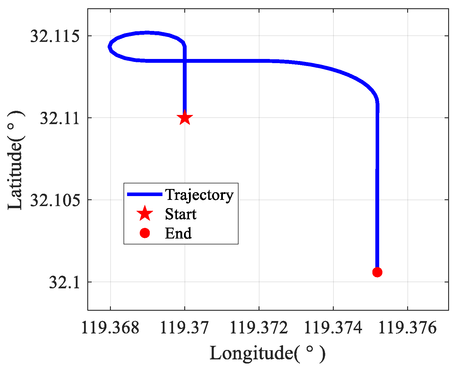
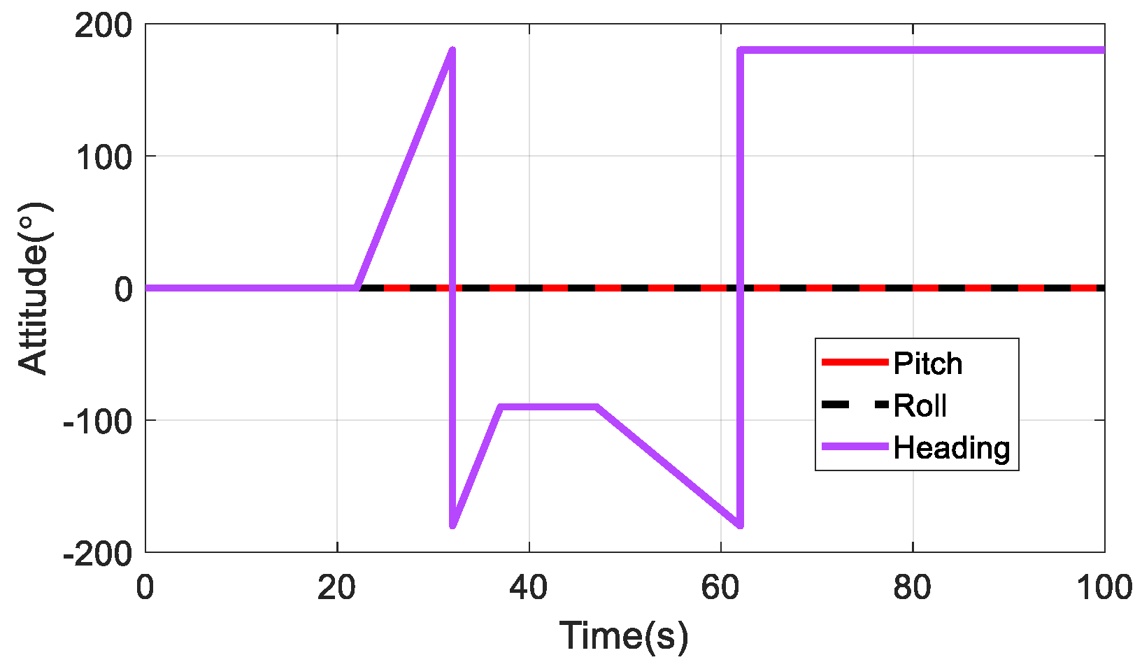
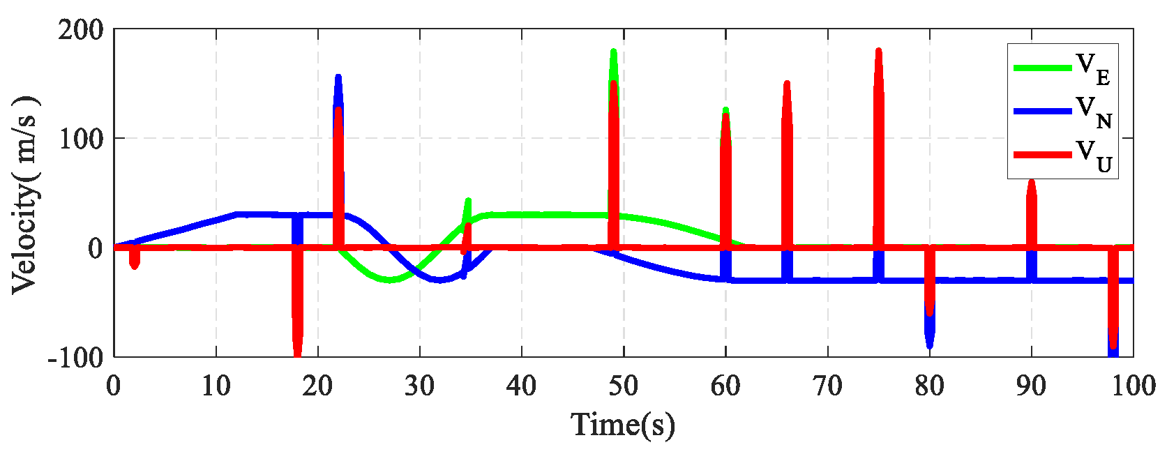
In this section, simulation analyses are carried out to evaluate the five methods described previously. The complete alignment process takes place over 100 s, starting with the vehicle positioned at 32.11°N and 119.37°E. Figure 3 and Figure 4 illustrate the vehicle’s trajectory and reference attitude, respectively. Additionally, Figure 5 illustrates the GNSS velocity output affected by outliers.
The sampling frequency of the three-axis gyroscopes and three-axis accelerometers in the SINS was set at 100 Hz. The constant biases of the gyroscopes were 0.1 ° / s , and the gyroscopes’ random biases were 0.05 ° / s . The constant biases of the accelerometers were 500 μ g , and the acceleration random biases were 100 μ g . The GNSS sampling frequency was set at 1 Hz. Due to signal reflections from tunnel/high-rise scenes and occlusions by obstacles in complex urban environments, the noise in real-world GNSS measurements exhibits significant heavy-tailed behavior. Therefore, a Gaussian mixture noise model was adopted to simulate the noise in GNSS velocity output, which is represented as follows:
δ v n = N ( 0 , ( 0.1 ) 2 I ) w . p .0.97 N ( 0 , ( 50 ) 2 I ) w . p .0.03
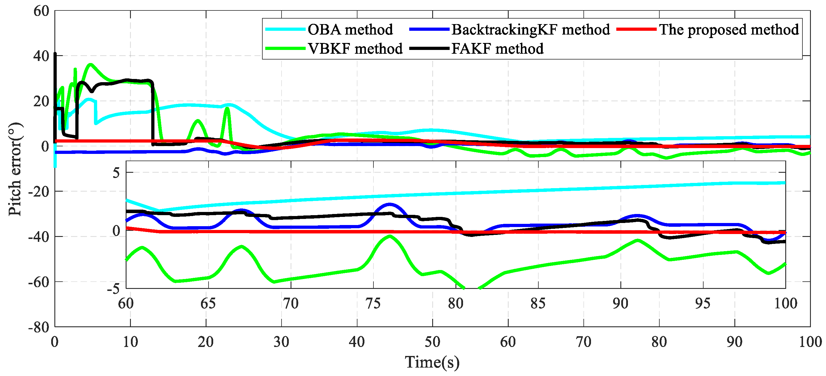
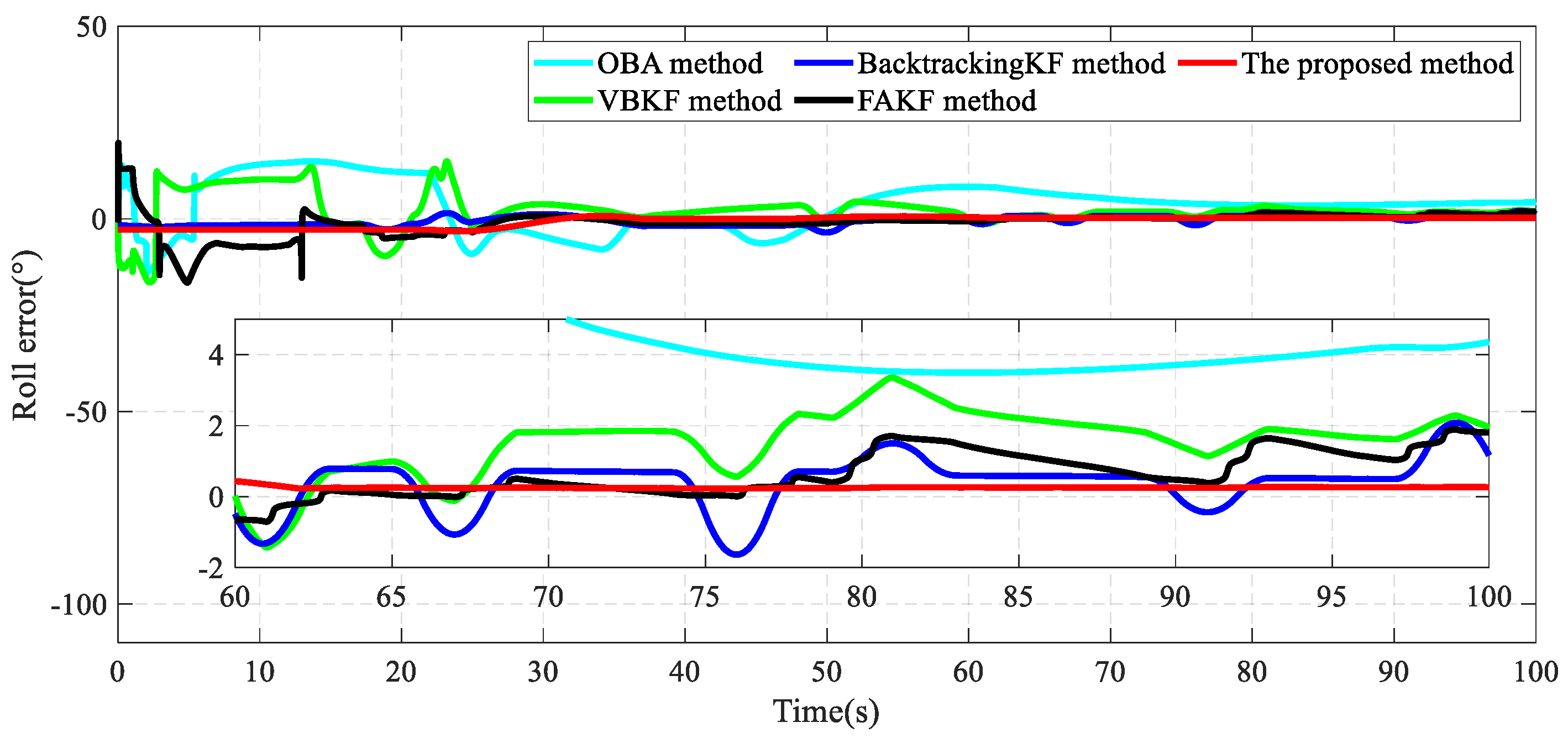
Figure 6 and Figure 7 show the pitch and roll errors for the five methods under comparison. As shown in Figure 6 and Figure 7, the conventional OBA and VBKF methods exhibit divergence in pitch and roll, while the other three methods achieve convergence. This result mainly occurs because the OBA method neglects errors in the inertial sensors and does not consider the outliers in GNSS. Significant fluctuations are observed in the initial estimation results of both the VBKF and FAKF methods, mainly because sensor parameters have not been accurately estimated at this stage. In contrast, the proposed method achieves improved accuracy and stability from the early stage of alignment, owing to the adaptive multiple backtracking approach. The presence of outliers leads to varying degrees of performance degradation in the VBKF, BKF, and FAKF methods. Taking the pitch error as an example, at 75 s, the VBKF method exhibits a 2.5° fluctuation lasting for 3 s. The BKF method shows a 1.8° fluctuation over the same duration, and the FAKF method also experiences disturbances. While the convergence accuracy of the above methods is degraded by outliers, the proposed method exhibits strong robustness and maintains stable convergence throughout the alignment process.
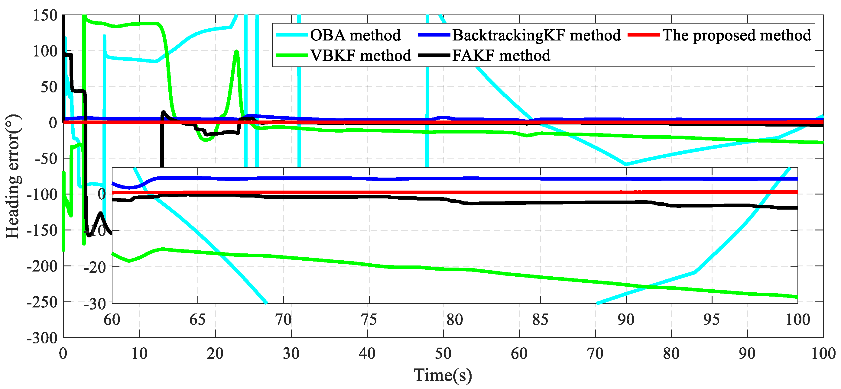
As illustrated by the heading errors in Figure 8, the OBA and VBKF methods fail to achieve convergence during the alignment process. During the initial stage, the FAKF method exhibits significant estimation fluctuations lasting approximately 30 s. In contrast, the BKF method and the proposed method exhibit stable convergence characteristics in the initial stage. Experimental data show that the heading error of the BKF method is approximately 5°, and the proposed method is approximately 1°. During the later stage, the heading error of the proposed method stabilizes within 0.8°, whereas the FAKF and BKF methods stabilize within 5° and 4°, respectively. Although the FAKF method employs magnitude matching to mitigate the effect of outliers, the limited amount of IMU and GNSS data acquired during short-term in-motion alignment restricts its ability to achieve higher accuracy. The BKF method extends the navigation data to obtain a smoother alignment result by utilizing a standard backtracking approach. However, its performance remains susceptible to outliers and noise with varying statistical characteristics. In contrast, the proposed method maintains both stability and high accuracy throughout the alignment process. Even when the GNSS-aided velocity measurements contain outliers, the heading errors remain stable, without any abrupt jumps. This conclusion is further corroborated by the roll and pitch error curves shown in Figure 6 and Figure 7.
To demonstrate the performance of the aforementioned alignment methods more clearly, Table 2 summarizes the mean and standard deviation (STD) of the attitude errors over the interval from 60 s to 100 s. The proposed method achieves an STD of less than 0.05° across all three attitude angles, where the FAKF method is around 1° and the BKF method is around 0.7°. Based on the profile toolbox of MATLAB 2022a, the running time of the proposed method in the simulation test is 3.79 s. From these statistical results, it is obvious that the proposed method offers superior stability and higher alignment accuracy compared to the other methods. Enhanced stability benefits from the residual-based reconstruction of the observation vector, which enables effective outlier isolation and detection.
Additionally, the designed adaptive multiple backtracking approach not only extends the length of available IMU and GNSS data but also maintains the filter’s tracking sensitivity and unbiasedness, thereby fully exploiting the available information and shortening the alignment time. Furthermore, the EM-based robust Kalman filter enables real-time adjustment of the measurement noise covariance matrix and the predicted error covariance matrix, effectively addressing the issue of inaccurate noise modeling and enhancing the estimation accuracy.

4.2. Field Test

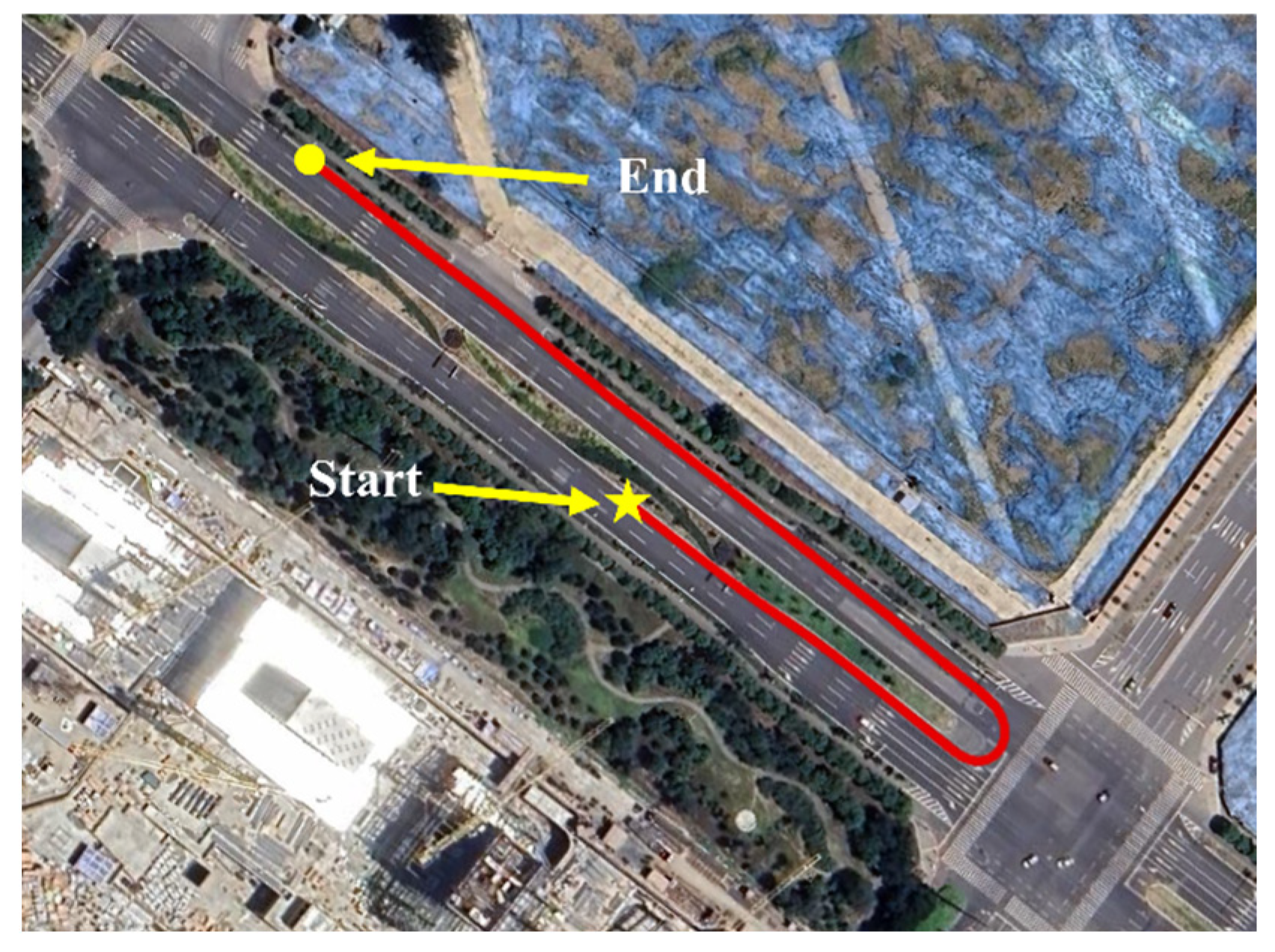
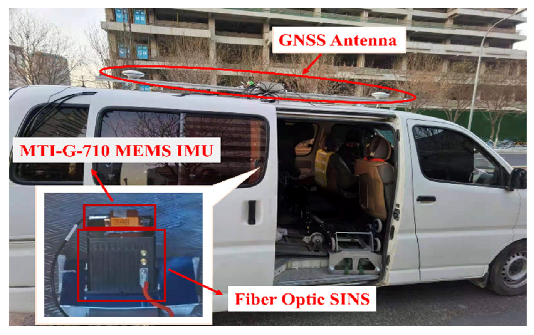
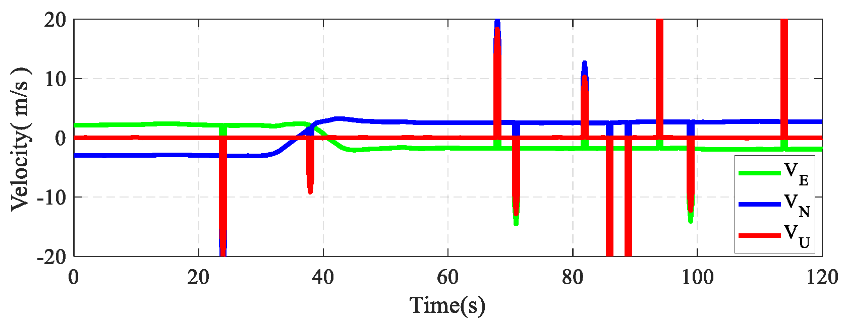
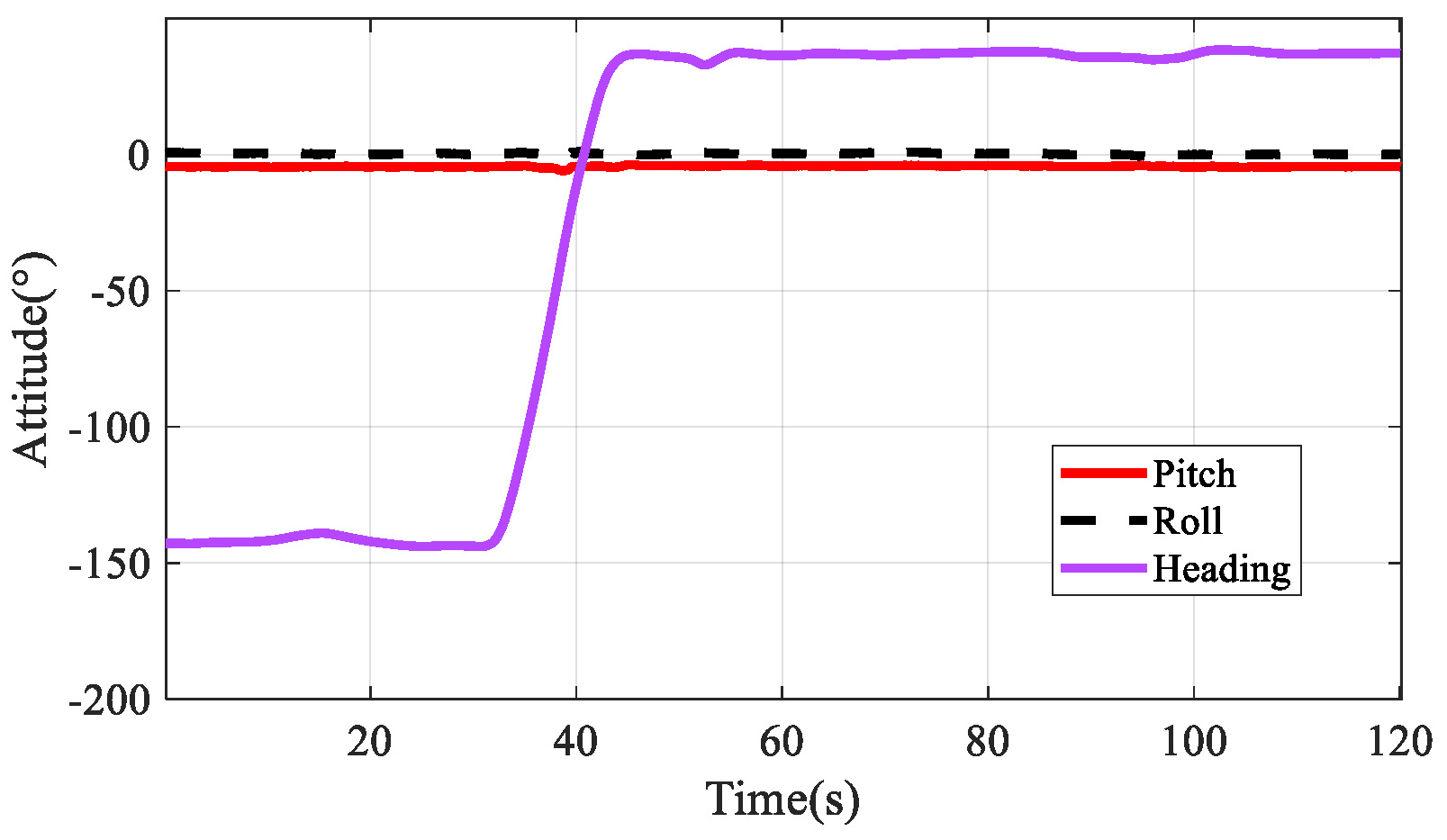
To further demonstrate the effectiveness and advantages of the proposed method, this section provides experimental validation using field test data. The test vehicle starts from an initial position at 39.7°N latitude and 116.5°E longitude, and the alignment process lasts for 120 s. The trajectory of the vehicle is shown in Figure 9. The experimental setup is illustrated in Figure 10, which comprises a Micro-Electromechanical Systems (MEMS) IMU, a fiber-optic SINS, and a GNSS receiver. The MEMS IMU employed is the MTI-G-710, with sensor specifications provided in Table 3. Figure 11 presents the GNSS velocity output affected by outliers. Figure 12 shows the attitude output by the high-accuracy fiber-optic SINS/GNSS navigation system, which serves as the reference.
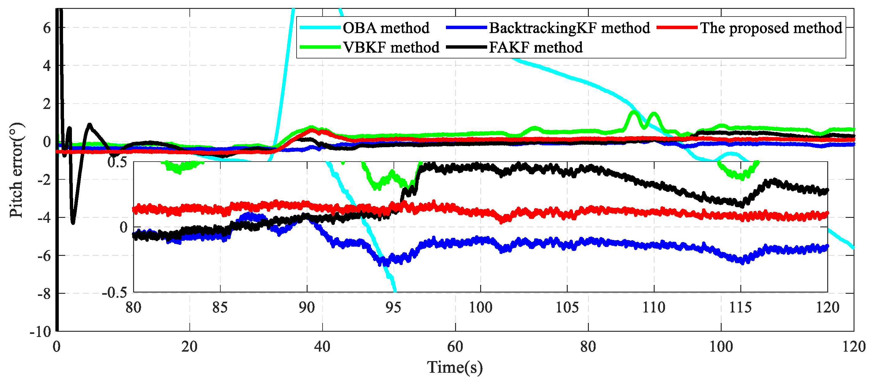
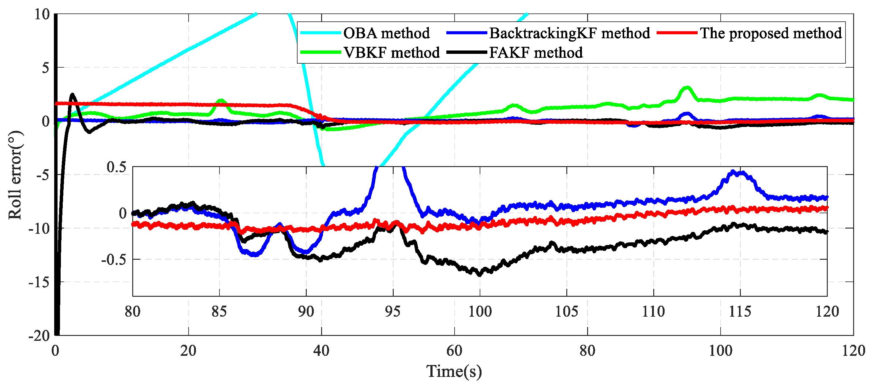
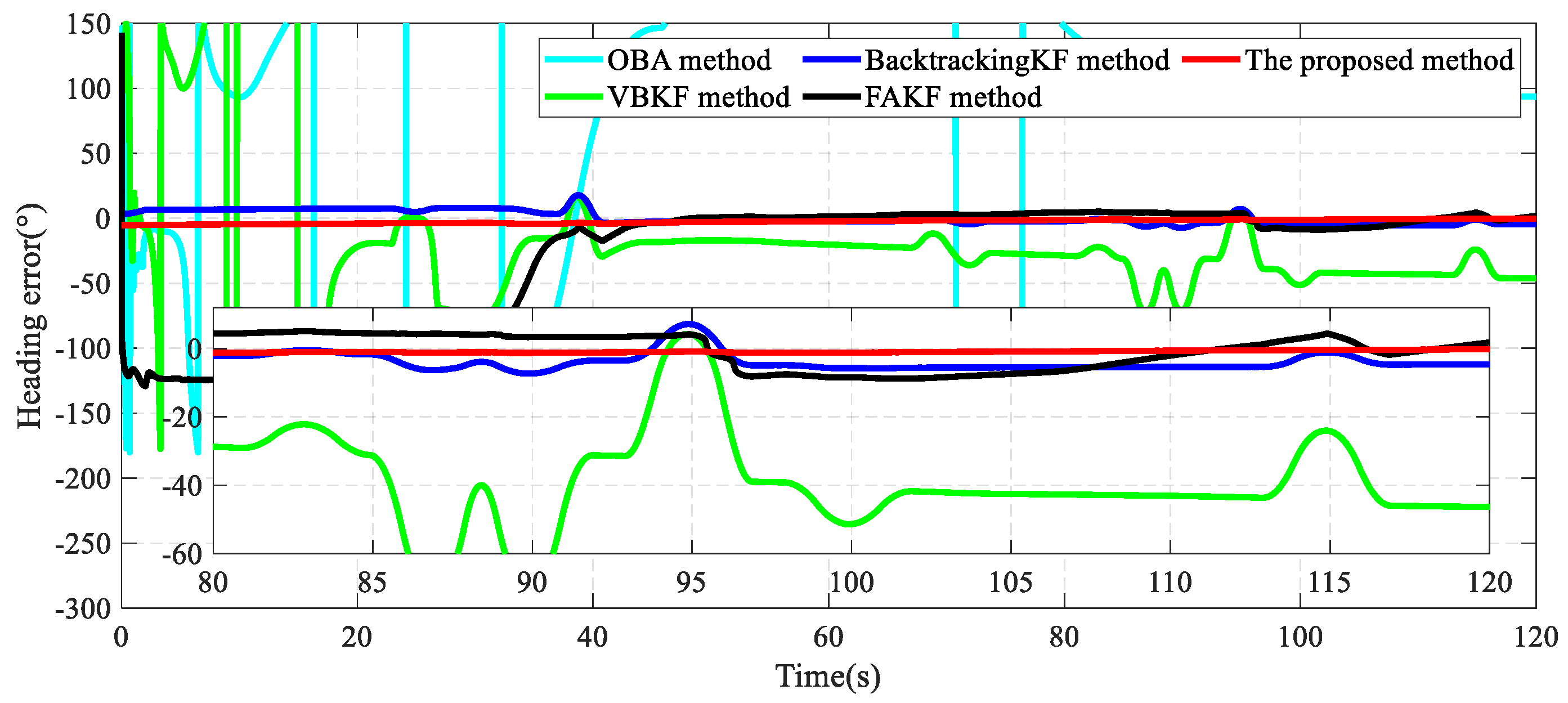
Figure 13, Figure 14 and Figure 15 present the attitude error curves for the five methods. The OBA method exhibits divergence in all three attitude angles. The pitch error of the VBKF method shows high variability, and the estimation accuracy is significantly lower compared to other methods. Furthermore, the roll and heading errors show divergent trends during the field test. In contrast, the remaining three methods achieve convergence in all three attitude angles. However, both the BKF and FAKF methods exhibit varying degrees of abrupt jumps as a result of outlier interference. The proposed method demonstrates a clear advantage in stability and accuracy. Taking the heading error as the critical evaluation indicator, it can be observed that after 80 s, the maximum heading error of the BKF method reached 7.3°, and that of the FAKF method reached 8°. In contrast, the proposed method stabilized the heading error within 1.2°.
Table 4 summarizes the statistical characteristics of the alignment results for the five methods over the interval from 80 s to 120 s. The proposed method achieves STD of less than 0.8° for roll and pitch errors, representing improvements of 63% and 57% over the BKF and FAKF methods, respectively. The heading error STD of the proposed method is 0.31°, which represents an improvement of over 2° compared to the other methods. In the later stages of the alignment process, around 95 and 115 s, the BKF and FAKF methods exhibited abrupt jumps due to outliers in the measurement data. In contrast, the proposed method maintains a more stable heading error around 0.8°. Based on the profile toolbox of MATLAB 2022a, the running time of the proposed method in the field test is 4.11 s. Overall, the proposed in-motion alignment algorithm demonstrates superior accuracy and enhanced robustness against disturbances.
The statistical results indicate that the proposed method significantly reduces the alignment time while achieving high alignment accuracy. This result can be attributed to two aspects. On the one hand, an adaptive window adjustment approach is applied to process the navigation data, in which an innovation gradient is used to distinguish windows with different noise statistical characteristics. By incorporating the multiple backtracking mechanism, this approach improves the utilization of navigation data, thereby effectively shortening the alignment time. On the other hand, the sliding window method mitigates the accumulation of sensor errors. By reconstructing the observation vector using the residual, the proposed method effectively isolates outliers from the GNSS velocity output. Meanwhile, the incorporation of the VB and EM methods mitigates the inaccuracies in the predicted error covariance matrix and the measurement noise covariance matrix, thereby enhancing the robustness of the filtering process in complex environments. The combination of these two aspects enables a reduction in in-motion alignment time and enhances alignment accuracy.

5. Conclusions

This paper proposes an adaptive multiple backtracking robust in-motion alignment method of low-cost SINS/GNSS for autonomous vehicles. An outlier suppression strategy based on the magnitude matching method is designed to mitigate the effect of outliers. An adaptive window adjustment multiple backtracking approach is proposed to effectively utilize navigation data and significantly shorten the alignment time in complex environments. By intelligently determining the size of the backtracking window, the proposed method effectively improves alignment accuracy. Finally, an EM-based robust variational Bayesian Kalman filter is proposed to improve attitude estimation accuracy. Simulation and experimental results demonstrate that the proposed method offers significant advantages in stability and alignment time. The proposed method completes alignment within 120 s and achieves higher alignment accuracy compared to other methods within the same alignment time. After 80 s, the heading error of the BKF method remains within 4°, while that of the FAKF method remains within 7°. In contrast, the proposed method converges with a heading error within 2.3°. Compared with existing methods, the proposed method can rapidly achieve the alignment accuracy required for navigation within a short duration. Hence, the proposed method is applicable to autonomous vehicles equipped with low-cost SINS. Reliable alignment under transient GNSS signal interruptions in complex environments will be addressed in future research.

Author Contributions

Conceptualization, W.L.; formal analysis, X.T.; funding acquisition, X.T.;methodology, W.L. and Y.W.; project administration, S.J.; software, Y.W.; supervision, H.H.; validation, Y.W.; writing—original draft, W.L. and Y.W.; writing—review and editing, S.J. and J.W. All authors have read and agreed to the published version of the manuscript.

Funding

This work was partially supported by the Jiangsu Province Higher Education Basic (Natural Science) Research Project under Grant 22KJB510018, the China Postdoctoral Science Foundation under Grant 2025M770240, the Tianjin Key Research and Development Program under Grant 24YFYSHZ00110, and the Postgraduate Research and Practice Innovation Program of Jiangsu Province under Grant KYCX25_4379.

Data Availability Statement

The raw and processed data necessary to replicate these findings cannot be shared currently, as it is part of an ongoing study.

Acknowledgments

The authors would like to thank B. Liu for providing the test data.

Conflicts of Interest

The authors declare no conflicts of interest.

References

  1. Wu, P.; Nie, W.; Liu, Y.; Xu, T. Improving the underwater navigation performance of an IMU with acoustic long baseline calibration. Satell. Navig. 2024, 5, 7. [Google Scholar] [CrossRef]
  2. Han, S.; Wang, J. A novel initial alignment scheme for low-cost INS aided by GPS for land vehicle applications. J. Navig. 2010, 63, 663–680. [Google Scholar] [CrossRef]
  3. Wang, K.; Xu, X.; Gao, W.; Wang, J. Linearized in-motion alignment for a low-cost INS. IEEE Trans. Aerosp. Electron. Syst. 2019, 56, 1917–1925. [Google Scholar] [CrossRef]
  4. Chen, Z.; Liu, Y.; Liu, S.; Wang, S.; Yang, L. An Improved Fading Factor-Based Adaptive Robust Filtering Algorithm for SINS/GNSS Integration with Dynamic Disturbance Suppression. Remote Sens. 2025, 17, 1449. [Google Scholar] [CrossRef]
  5. Xu, X.; Gui, J.; Sun, Y.; Yao, Y.; Zhang, T. A Robust In-Motion Alignment Method With Inertial Sensors and Doppler Velocity Log. IEEE Trans. Instrum. Meas. 2021, 70, 3011873. [Google Scholar] [CrossRef]
  6. Xu, T.; Xu, X.; Xu, D.; Zou, Z.; Zhao, H. A new robust filtering method of GNSS/MINS integrated system for land vehicle navigation. IEEE Trans. Veh. Technol. 2022, 71, 11443–11453. [Google Scholar] [CrossRef]
  7. Huang, Y.; Zhang, Y.; Chang, L. A New Fast In-Motion Coarse Alignment Method for GPS-Aided Low-Cost SINS. IEEE/ASME Trans. Mechatron. 2018, 23, 1303–1313. [Google Scholar] [CrossRef]
  8. Huang, Y.; Zhang, Z.; Du, S.; Li, Y.; Zhang, Y. A high-accuracy GPS-aided coarse alignment method for MEMS-based SINS. IEEE Trans. Instrum. Meas. 2020, 69, 7914–7932. [Google Scholar] [CrossRef]
  9. Wei, J.; Yu, F.; Fan, S.; Zhang, Y.; Wang, Y.; Wang, Y. A Robust In-Motion Alignment Method for a DVL-Aided SINS With Latitude Uncertainty. IEEE Trans. Instrum. Meas. 2024, 73, 3341141. [Google Scholar] [CrossRef]
  10. Zhou, X.; Zhang, M.; Hu, J.; Li, L.; Guan, X. A Robust In-Motion Coarse Alignment Method for Low-Accuracy SINS and GPS Integrated System. IEEE/ASME Trans. Mechatron. 2025, 30, 611–622. [Google Scholar] [CrossRef]
  11. Sun, X.; Zhuang, Y.; Yang, X.; Huai, J.; Huang, T.; Feng, D. Tightly coupled VLP/INS integrated navigation by inclination estimation and blockage handling. Satell. Navig. 2025, 6, 7. [Google Scholar] [CrossRef]
  12. Xu, X.; Zheng, X.; Li, Y.; Yao, Y.; Zhou, H.; Zhu, L. An Improved In-Motion Alignment Method for SINS/GPS with the Sliding Windows Integration. IEEE Trans. Veh. Technol. 2023, 72, 12491–12499. [Google Scholar] [CrossRef]
  13. Xu, X.; Li, Y.; Zhu, L.; Yao, Y. Robust attitude and positioning alignment methods for SINS/DVL integration based on sliding window improvements. IEEE Trans. Ind. Electron. 2023, 71, 8038–8046. [Google Scholar] [CrossRef]
  14. Zhu, Y.; Zhang, T.; Cui, B.; Wei, X.; Jin, B. In-Motion Coarse Alignment for SINS/USBL Based on USBL Relative Position. IEEE Trans. Autom. Sci. Eng. 2025, 22, 1425–1434. [Google Scholar] [CrossRef]
  15. Jin, S.; Camps, A.; Jia, Y.; Wang, F.; Martin-Neira, M.; Huang, F.; Yan, Q.; Zhang, S.; Li, Z.; Edokossi, K. Remote sensing and its applications using GNSS reflected signals: Advances and prospects. Satell. Navig. 2024, 5, 19. [Google Scholar] [CrossRef]
  16. Sun, J.; Chen, Z.; Wang, F. A novel ML-aided methodology for SINS/GPS integrated navigation systems during GPS outages. Remote Sens. 2022, 14, 5932. [Google Scholar] [CrossRef]
  17. Wu, M.; Wu, Y.; Hu, X.; Hu, D. Optimization-based alignment for inertial navigation systems: Theory and algorithm. Aerosp. Sci. Technol. 2011, 15, 1–17. [Google Scholar] [CrossRef]
  18. Wu, Y.; Pan, X. Velocity/position integration formula part I: Application to in-flight coarse alignment. IEEE Trans. Aerosp. Electron. Syst. 2013, 49, 1006–1023. [Google Scholar] [CrossRef]
  19. Xu, X.; Sun, Y.; Yao, Y.; Zhang, T. A robust in-motion optimization-based alignment for SINS/GPS integration. IEEE Trans. Intell. Transp. Syst. 2021, 23, 4362–4372. [Google Scholar] [CrossRef]
  20. Wang, J.; Chen, X.; Shao, X. An adaptive multiple backtracking UKF method based on Krein space theory for marine vehicles alignment process. IEEE Trans. Veh. Technol. 2022, 72, 3214–3226. [Google Scholar] [CrossRef]
  21. Cao, S.; Bian, Y.; Wang, G.; Qin, H.; Hu, M.; Cui, Q.; Ding, R. Velocity-Integral-Constraint-based In-Motion Initial Alignment for Kalman Filter-Aided Low-Cost SINS. IEEE Trans. Instrum. Meas. 2025, 74, 8506313. [Google Scholar] [CrossRef]
  22. Wei, X.; Li, J.; Han, D.; Wang, J.; Zhan, Y.; Wang, X.; Feng, K. An in-flight alignment method for global positioning system-assisted low cost strapdown inertial navigation system in flight body with short-endurance and high-speed rotation. Remote Sens. 2023, 15, 711. [Google Scholar] [CrossRef]
  23. Wang, J.; Chen, X.; Liu, J.; Zhu, X.; Zhong, Y. A Robust Backtracking CKF Based on Krein Space Theory for In-Motion Alignment Process. IEEE Trans. Intell. Transp. Syst. 2022, 24, 1909–1925. [Google Scholar] [CrossRef]
  24. Chang, L.; Hu, B.; Li, Y. Backtracking integration for fast attitude determination-based initial alignment. IEEE Trans. Instrum. Meas. 2014, 64, 795–803. [Google Scholar] [CrossRef]
  25. Fu, Q.; Li, S.; Liu, Y.; Wu, F. Information-reusing alignment technology for rotating inertial navigation system. Aerosp. Sci. Technol. 2020, 99, 105747. [Google Scholar] [CrossRef]
  26. Lin, Y.; Miao, L.; Zhou, Z. A high-accuracy initial alignment method based on backtracking process for strapdown inertial navigation system. Measurement 2022, 201, 111712. [Google Scholar] [CrossRef]
  27. Wei, X.; Li, J.; Feng, K.; Zhang, D. An Improved In-flight Alignment Method Based on Backtracking Navigation for GPS-aided Low Cost SINS With Short Endurance. IEEE Robot. Autom. Lett. 2022, 7, 634–641. [Google Scholar] [CrossRef]
  28. Wang, D.; Wang, B.; Huang, H.; Xu, B.; Zhang, H. A Novel SINS/DVL Integrated Navigation Method Based on Different Track Models for Complex Environment. IEEE Trans. Instrum. Meas. 2024, 73, 3373066. [Google Scholar] [CrossRef]
  29. Zhang, L.; Zhang, T.; Wei, H. A Factor Graph Optimization-Based In-motion Alignment Method for INS/DVL Integration. IEEE Trans. Veh. Technol. 2024, 73, 18452–18459. [Google Scholar] [CrossRef]
  30. Jarraya, I.; Al-Batati, A.; Kadri, M.B.; Abdelkader, M.; Ammar, A.; Boulila, W.; Koubaa, A. Gnss-denied unmanned aerial vehicle navigation: Analyzing computational complexity, sensor fusion, and localization methodologies. Satell. Navig. 2025, 6, 9. [Google Scholar] [CrossRef]
  31. Huang, Y.; Zhang, Y.; Wu, Z.; Li, N.; Chambers, J. A Novel Adaptive Kalman Filter With Inaccurate Process and Measurement Noise Covariance Matrices. IEEE Trans. Autom. Control 2018, 63, 594–601. [Google Scholar] [CrossRef]
  32. Du, S.; Zhu, F.; Wang, Z.; Huang, Y.; Zhang, Y. A Novel Lie Group Framework-based Student’s t Robust Filter and Its Application to INS/DVL Tightly Integrated Navigation. IEEE Trans. Instrum. Meas. 2024, 73, 3379400. [Google Scholar] [CrossRef]
  33. Chen, Y.; Li, W.; Du, Y. A novel robust adaptive Kalman filter with application to urban vehicle integrated navigation systems. Measurement 2024, 236, 114844. [Google Scholar] [CrossRef]
  34. Chen, H.; Sun, R.; Cheng, Q.; Yin, T.; Zhou, Y.; Ochieng, W.Y. GNSS/IMU/LO integration with a new LO error model and lateral constraint for navigation in urban areas. Satell. Navig. 2024, 5, 30. [Google Scholar] [CrossRef]
  35. Sun, J.; Ye, Q.; Lei, Y. In-motion alignment method of SINS based on improved Kalman filter under geographic latitude uncertainty. Remote Sens. 2022, 14, 2581. [Google Scholar] [CrossRef]
  36. Ge, B.; Zhang, H.; Fu, W.; Yang, J. Enhanced Redundant Measurement-Based Kalman Filter for Measurement Noise Covariance Estimation in INS/GNSS Integration. Remote Sens. 2020, 12, 3500. [Google Scholar] [CrossRef]
  37. Lyu, W.; Meng, F.; Jin, S.; Zeng, Q.; Wang, Y.; Wang, J. Robust In-Motion Alignment of Low-Cost SINS/GNSS for Autonomous Vehicles Using IT2 Fuzzy Logic. IEEE Internet Things J. 2025, 12, 9996–10011. [Google Scholar] [CrossRef]
  38. Shi, W.; Xu, J.; He, H.; Li, D.; Tang, H.; Lin, E. Fault-tolerant SINS/HSB/DVL underwater integrated navigation system based on variational Bayesian robust adaptive Kalman filter and adaptive information sharing factor. Measurement 2022, 196, 111225. [Google Scholar] [CrossRef]
  39. Huang, Y.; Zhang, Y.; Li, N.; Wu, Z.; Chambers, J.A. A novel robust student’s t-based Kalman filter. IEEE Trans. Aerosp. Electron. Syst. 2017, 53, 1545–1554. [Google Scholar] [CrossRef]
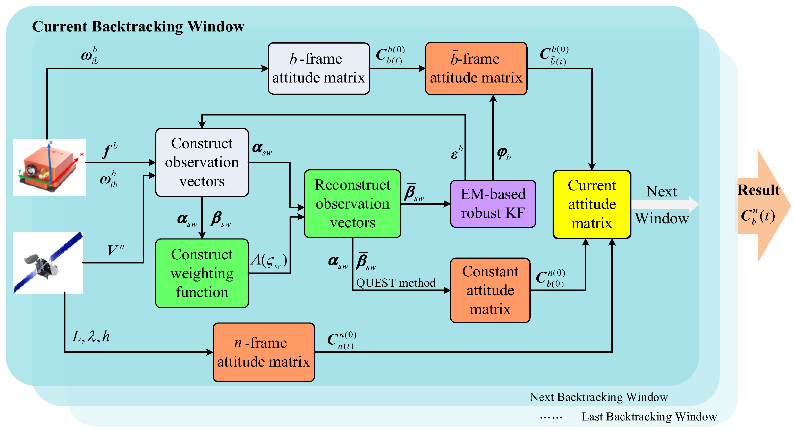
Figure 1. Diagram of the proposed multiple backtracking in-motion alignment method.
Remotesensing 17 02680 g001
Figure 2. Diagram of the proposed adaptive multiple backtracking approach.
Remotesensing 17 02680 g002
Figure 3. Vehicle’s trajectory in the simulation test.
Remotesensing 17 02680 g003
Figure 4. Reference attitude in the simulation test.
Remotesensing 17 02680 g004
Figure 5. Velocity from the GNSS output in the simulation test.
Remotesensing 17 02680 g005
Figure 6. Pitch errors of five methods in the simulation test.
Remotesensing 17 02680 g006
Figure 7. Roll errors of five methods in the simulation test.
Remotesensing 17 02680 g007
Figure 8. Heading errors of five methods in the simulation test.
Remotesensing 17 02680 g008
Figure 9. Vehicle’s trajectory in the field test.
Remotesensing 17 02680 g009
Figure 10. Experimental vehicle and related equipment.
Remotesensing 17 02680 g010
Figure 11. Velocity from the GNSS output in the field test.
Remotesensing 17 02680 g011
Figure 12. Reference attitude in the field test.
Remotesensing 17 02680 g012
Figure 13. Pitch errors of five methods in the field test.
Remotesensing 17 02680 g013
Figure 14. Roll errors of five methods in the field test.
Remotesensing 17 02680 g014
Figure 15. Heading errors of five methods in the field test.
Remotesensing 17 02680 g015
Table 1. Nomenclature.
NotationsDefinitions
i Inertial frame
n Navigation frame
b True body frame
b ˜ Calculated body frame
g n Gravity vector
f b Specific force
ε b Gyroscope constant biases
C b a Attitude matrix from b frame to a frame
ω b c a Angular rate of b frame related to c frame projected in a
V n Ground velocity of the SINS in n frame
I 3 3 × 3 identity matrix
( a ) × Skew symmetric matrix of vector a
( ) T Transpose operation
t r ( ) Trace operation
Table 2. The 60~100 s attitude error statistical characteristics.
Evaluating IndicatorAttitude Error (°)OBAVBKFBKFFAKFProposed
MeanPitch5.534−2.9560.5300.636−0.122
Roll4.6531.5610.4050.6690.257
Heading−27.446−21.2653.951−1.8900.337
STDPitch0.2741.0810.5660.7650.049
Roll1.4140.9170.7350.6380.026
Heading18.7193.8980.4681.0740.037
Table 3. MTI-G-710 sensor specifications.
IndexGyroscopeAccelerometer
Update rate100 Hz100 Hz
Standard full range±450°/s±20 g
Initial bias error0.2°/s5 mg
In-run bias stability10°/h15 μg
Noise density0.01°/s/√Hz60 μg/√Hz
Table 4. The 80~120 s attitude error statistical characteristics.
Evaluating
Indicator
Attitude Error (°)OBAVBKFBKFFAKFProposed
MeanPitch−1.0680.668−0.1190.2270.120
Roll24.3931.9020.058−0.284−0.088
Heading102.960−39.164−3.8694.4230.870
STDPitch2.4480.2550.0780.1810.079
Roll5.1580.3910.2140.1870.079
Heading11.17214.3982.6715.0340.314
Disclaimer/Publisher’s Note: The statements, opinions and data contained in all publications are solely those of the individual author(s) and contributor(s) and not of MDPI and/or the editor(s). MDPI and/or the editor(s) disclaim responsibility for any injury to people or property resulting from any ideas, methods, instructions or products referred to in the content.