Potential of Multi-Source Multispectral vs. Hyperspectral Remote Sensing for Winter Wheat Nitrogen Monitoring

Abstract

Timely and accurate monitoring of crop nitrogen (N) status is essential for precision agriculture. UAV-based hyperspectral remote sensing offers high-resolution data for estimating plant nitrogen concentration (PNC), but its cost and complexity limit large-scale application. This study compares the performance of UAV hyperspectral data (S185 sensor) with simulated multispectral data from DJI Phantom 4 Multispectral (P4M), PlanetScope (PS), and Sentinel-2A (S2) in estimating winter wheat PNC. Spectral data were collected across six growth stages over two seasons and resampled to match the spectral characteristics of the three multispectral sensors. Three variable selection strategies (one-dimensional (1D) spectral reflectance, optimized two-dimensional (2D), and three-dimensional (3D) spectral indices) were combined with Random Forest Regression (RFR), Support Vector Machine Regression (SVMR), and Partial Least Squares Regression (PLSR) to build PNC prediction models. Results showed that, while hyperspectral data yielded slightly higher accuracy, optimized multispectral indices, particularly from PS and S2, achieved comparable performance. Among models, SVM and RFR showed consistent effectiveness across strategies. These findings highlight the potential of low-cost multispectral platforms for practical crop N monitoring. Future work should validate these models using real satellite imagery and explore multi-source data fusion with advanced learning algorithms.

1. Introduction

Wheat (Triticum aestivum L.) is a fundamental crop for global food security [1]. Achieving high yields of winter wheat typically requires substantial nitrogen (N) fertilizer inputs. However, excessive N application can lead to serious environmental issues, including greenhouse gas emissions and water contamination [2]. Plant N concentration (PNC) serves as a key indicator of crop N status and plays a crucial role in guiding precision N fertilizer management strategies [3]. Hence, timely and accurate assessment of crop PNC is essential for sustainable agricultural practices.

Traditional methods for determining crop PNC involve field destructive sampling and laboratory chemical analysis. Although highly accurate, they are time-consuming and costly, making them impractical for large-scale crop N monitoring. In contrast, remote sensing technologies have emerged as a powerful non-destructive alternative, playing an increasingly important role in monitoring crop nitrogen status over the past few decades [4]. With the advancements in unmanned aerial vehicle (UAV) and satellite technologies, remote sensing has emerged as a key tool for monitoring crop growth and nutritional status [5].

UAV hyperspectral remote sensing provides spectral reflectance data across adjacent narrow bands, delivering detailed spectral information of crop canopy characteristics [6], which was widely applied in the estimation of winter wheat canopy N density [7] and soil moisture [8]. However, the high cost, limited coverage, and complex data processing processes of UAV hyperspectral remote sensing limit its application. In comparison, UAV multispectral sensors are easier to operate, less expensive, and involve simpler data processing, making them better suited for large-scale farm applications [9]. Despite their practicality, multispectral UAVs have only a few spectral bands, which may not provide enough detailed information for accurate crop N concentration estimations. In addition, the short flight time of most UAV remote sensing systems makes them challenging to apply on a large scale. The development of satellite remote sensing provides an opportunity to extend the methods established by UAV remote sensing to a regional scale. Applications include estimation of biomass [10], crop grain N uptake [11], and yield prognosis [12]. Although different types of sensors are widely used in crop monitoring, their differing capabilities in estimating N concentration have not been systematically evaluated. Balancing sensor accuracy, cost, and coverage has become a key challenge in crop N monitoring.

Hyperspectral sensors offer the benefit of having a large number of spectral bands, allowing for detailed and extensive spectral data, making one-dimensional (1D) spectral reflectance analysis the most intuitive approach for data analysis. However, hyperspectral data can suffer from the “curse of dimensionality” [13], where the high number of features relative to the available sample size can lead to model overfitting, increased computational burden, and reduced generalization capability. Moreover, although hyperspectral bands contain information for estimating crop N concentration, their performance can be easily affected by atmospheric conditions and other background factors.

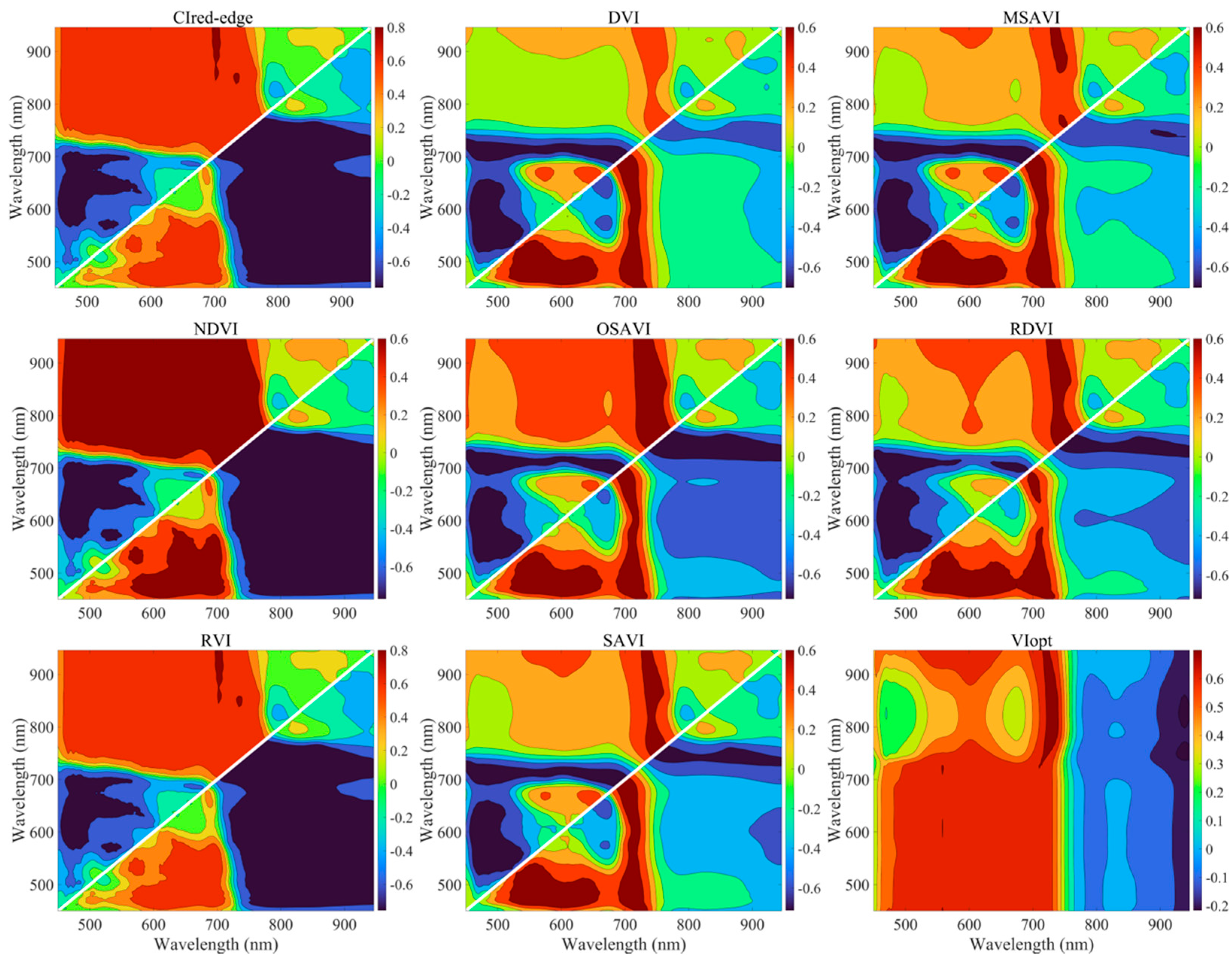
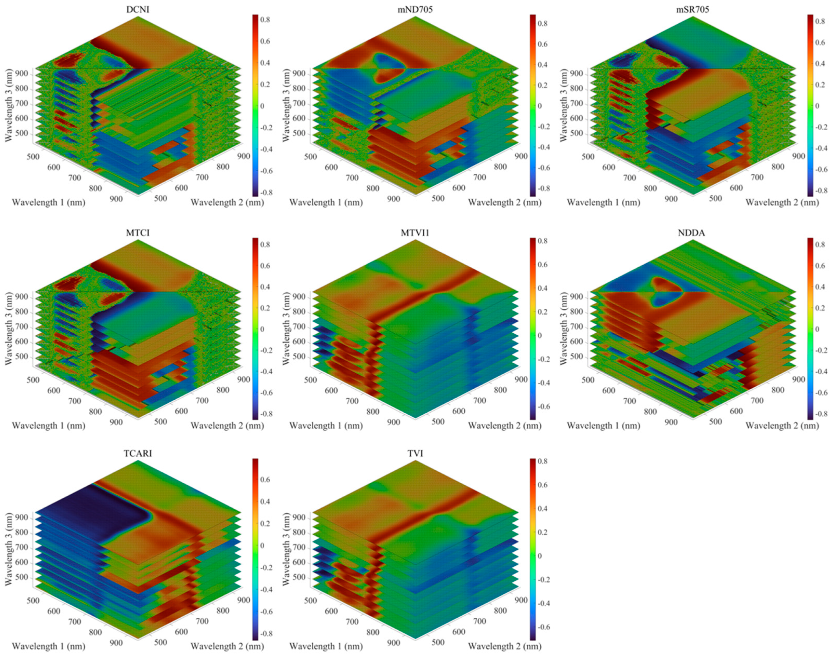
To improve robustness and simplify interpretation, researchers have increasingly focused on spectral indices, which are typically constructed from the reflectance values of two, three, or more specific bands [14]. The Normalized Difference Vegetation Index (NDVI) and the Ratio Vegetation Index (RVI) are the earliest and widely forms of two-dimensional (2D) spectral indices [15,16]. Building on this, researchers proposed a series of classical 2D spectral indices, including Soil-adjusted vegetation index (SAVI) [17], Modified soil-adjusted vegetation index (MSAVI) [18], Optimized soil-adjusted vegetation index (OSAVI) [19], etc. Recently, spectral indices constructed using three spectral bands, or three-dimensional (3D) spectral indices, have emerged as a promising approach to enhance the predictive capability of remote sensing models. Unlike traditional 1D reflectance or 2D spectral indices, 3D spectral indices can capture more complex spectral interactions and synergies among bands, potentially improving model performance for estimating crop biophysical parameters [20]. However, the 3D spectral indices proposed so far are still very limited, involving Double-peak Canopy Nitrogen Index (DCNI) [21] and Modified simple ratio index 705 (mSR705). Other 3D spectral indices have also been explored in recent studies, though they remain relatively few in number.

Although numerous spectral indices have shown promising results in diagnosing crop N status [21], their effectiveness may vary across crops, cultivars, regions, and growth stages. The N dilution effect and variation in canopy structure were the main reasons that interfered with crop N estimation accuracy and none of the traditional spectral indices could accurately predict crop PNC across the entire growing season [22]. Moreover, a traditional 2D or 3D spectral index is mostly a combination of bands selected by researchers under local conditions or based on experience. For hyperspectral sensors with numerous spectral bands, the traditional 2D or 3D spectral indices may omit spectral regions with critical spectral information [23], potentially compromising the accuracy of PNC estimation. Thus, there is an urgent need to optimize the traditional 2D or 3D spectral indices by systematically selecting sensitive band combinations and evaluating their predictive performance through correlation analysis and model validation. Guo et al. [24] estimated the potato canopy N content (CNC) based on an optimized 2D spectral index, and created a potato (Solanum tuberosum L.) CNC distribution map using UAV remote sensing. Fan et al. [25] compared and analyzed 1D UAV hyperspectral reflectance while also optimizing 2D and 3D spectral indices to estimate potato PNC, and found that the optimized 3D spectral index TBI5 outperformed the others, achieving the highest accuracy (R² = 0.65, RMSE = 0.39, NRMSE = 12.17%). Although multidimensional spectral indices led to considerable achievements in crop N monitoring, a comprehensive evaluation of multiple sensors for winter wheat PNC estimation remains unreported.

Recent research has emphasized the effectiveness of integrating machine learning (ML) models with remote sensing data to enhance the accuracy of crop N estimation [26,27]. Li et al. [28] demonstrated that partial least squares regression (PLSR) combined with spectral reflectance significantly improved the estimation accuracy of winter wheat CNC; Random forest regression (RFR) and support vector machine regression (SVMR) also showed promising results in that respect, especially when combined with optimized spectral indices [13].

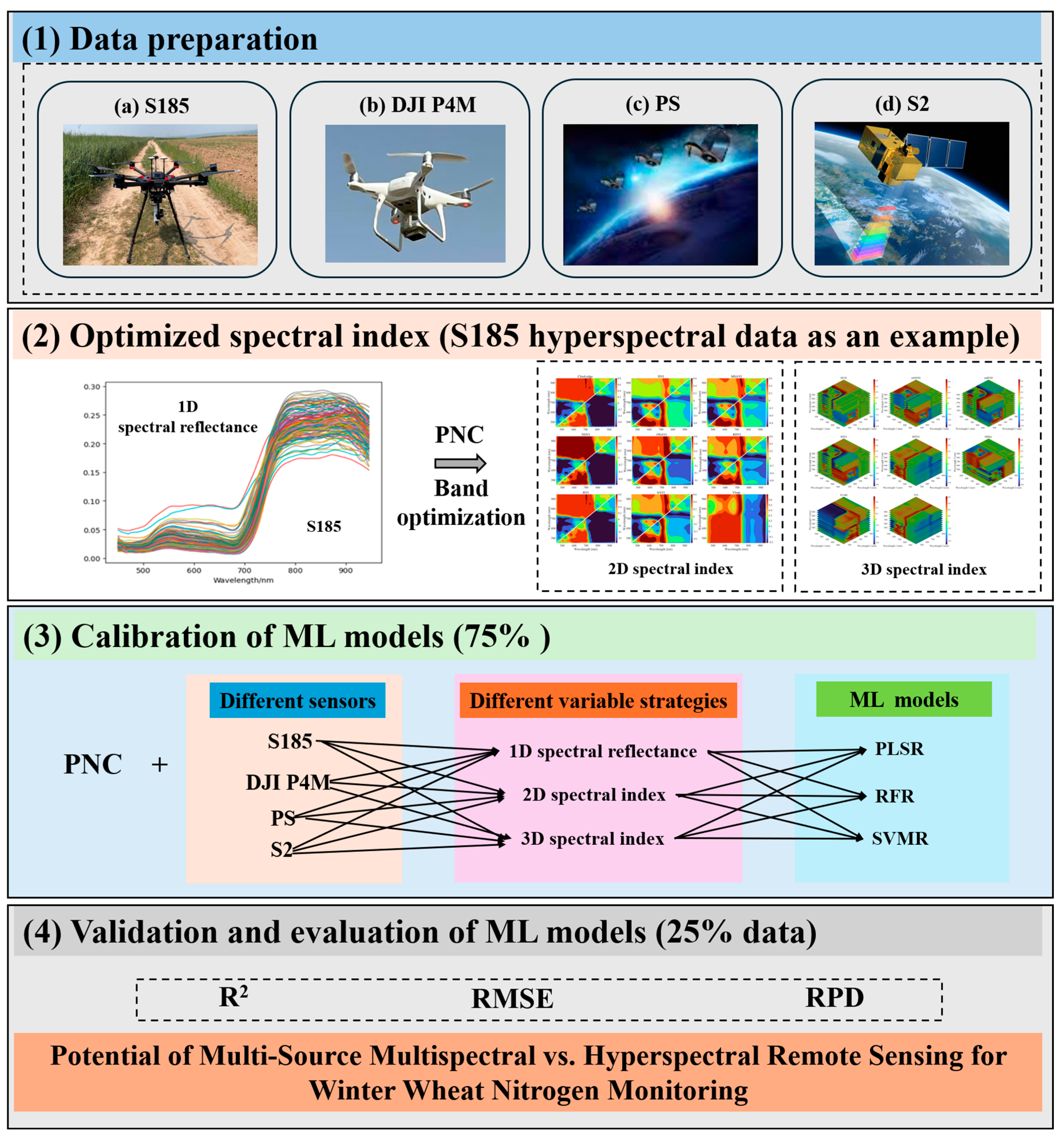
This study contributes to precision agriculture by systematically comparing the effectiveness of UAV hyperspectral, UAV multispectral, and satellite multispectral sensors for PNC estimation. By employing spectral resampling to simulate multispectral data for the popular platforms (DJI Phantom 4 Multispectral (DJI P4M), PlanetScope (PS) and Sentinel-2A (S2)) from the S185 UAV hyperspectral data, this study bridges the gap between high-precision UAV systems and scalable satellite remote sensing technologies. PNC estimation models were constructed using 1D spectral reflectance and optimized 2D and 3D spectral indices from different sensors combined with PLSR, RFR, and SVMR algorithms, respectively. The primary objective was to assess the potential of different remote sensing technologies for estimating winter wheat PNC, considering cost, accuracy, and regional applicability.

2. Materials and Methods

2.1. Experimental Design

Field experiments on winter wheat were conducted in Qian County, Shaanxi Province, China (108°07′E, 34°38′N), in 2017–2018 and 2021–2022 (Figure 1). Each experimental plot covered an area of 90 m² (9 m × 10 m), and a total of 36 plots were established in each season, resulting in 72 plots across the two experiments. The plots were designed with three N treatments, three phosphorus (P) treatments, and three potassium (K) treatments. All fertilizers were applied as basal fertilizer prior to planting, with no further fertilization occurred after planting. Winter wheat in this study was not irrigated and was planted according to local standard density. The management practices followed the conventional local standards, and any significant weed and insect infestations were recorded. Specific details of the two experiments are outlined in

Table 1. Details of the experiments conducted.

Experiment and Growing Season	Cultivar	N Rate (Kg/ha)	P Rate (Kg/ha)	K Rate (Kg/ha)	Sampling Date	Sampling Stage
Experiment 1 2017–2018	Xiaoyan 22	0, 30, 60, 90, 120, 150	0, 22.5, 45, 67.5, 90, 112.5	0, 22.5, 45, 67.5, 90, 112.5	07.05.2018	Flowering
					22.05.2018	Filling
Experiment 2 2021–2022	Xiaoyan 22	0, 60, 120, 180, 240, 300	0, 30, 60, 90, 120, 150	0, 30, 60, 90, 120, 150	10.04.2022	Booting
					25.04.2022	Heading
					07.05.2022	Flowering
					23.05.2022	Filling

.

2.2. Data Collection

2.2.1. UAV Hyperspectral Imagery Acquisition and Processing

A DJI M600Pro UAV (SZ DJI Technology Co., Shenzhen, China) equipped with a Cubert S185 hyperspectral imager (Cubert GmbH, Ulm, Germany) was used to capture hyperspectral images of winter wheat crops at different growth stages. The S185, a lightweight (470 g) full-frame spectrometer, captures 125 bands ranging from 450 to 950 nm, with a spectral sampling interval of 4 nm. Each image was obtained in just 1/1000 s. Before data collection, the system was calibrated using a reference target and dark current measurements. The UAV flew at 100 m altitude and 6 m/s speed, with a 30° field of view, ensuring sufficient overlap between images. Post-processing was conducted using Cubert Utils Touch software (Cubert GmbH) to merge hyperspectral and grayscale images. The resulting grayscale image was then georeferenced using ArcMap 10.6 (Esri, Redlands, CA, USA) and Google Earth (Google, Mountain View, CA, USA). The Region of Interest (ROI) tool in ENVI 5.3 (Harris Geospatial Solutions, Broomfield, CO, USA) was used to extract average reflectance data for specific sampling areas. The Savitzky–Golay smoothing technique was applied to reduce noise in the hyperspectral data. Imagery was acquired across six growth stages, with additional details in Table 1.

2.2.2. Winter Wheat PNC Measurement

After the S185 flight at each growth stage, a 0.5 m × 0.5 m sampling plot was selected, and the above-ground plant organs (including stems, leaves and spikes of winter wheat were harvested to measure PNC. The coordinates of the sampling locations were recorded using an RTK GPS system. The plant samples were first oven-dried at 105 °C for 30 min to halt metabolic activity, then dried further at 70 °C until their weight stabilized. Once dry, the samples were ground and analyzed for PNC using the modified Kjeldahl digestion method.

2.2.3. Multispectral Sensor Simulated Datasets

Based on the UAV S185 hyperspectral reflectance data (450–950 nm, 4 nm spectral resolution), three multispectral sensors were simulated, including DJI P4M, PS, and S2. The central wavelength and full width at half maximum (FWHM) values of each band are provided in

Table 2. The spectral bands of multispectral sensors simulated.

Sensor	Band Number	Band Name	Spectral Region (nm)	Country or Institution
DJI P4M	B1	Blue	450 ± 16	China
	B2	Green	560 ± 16
	B3	Red	650 ± 16
	B4	Red-edge	730 ± 16
	B5	Near infrared	840 ± 26
PS	B1 *	Coastal_blue	431–452	USA
	B2	Blue	465–515
	B3	Green_i	513–549
	B4	Green	547–583
	B5	Yellow	600–620
	B6	Red	650–680
	B7	Red edge	697–713
	B8	Near infrared	845–885
S2	B1 *	Coastal aerosol	433–453	ESA
	B2	Blue	458–523
	B3	Green	543–578
	B4	Red	650–680
	B5	Red-edge 1	698–713
	B6	Red-edge 2	733–748
	B7	Red-edge 3	773–793
	B8	Near infrared	785–900
	B8A	Near infrared narrow	855–875
	B9 *	Water vapour	935–955
	B10 *	Shortwave infrared/Cirrus	1360–1390
	B11 *	Shortwave infrared 1	1565–1655
	B12 *	Shortwave infrared 2	2100–2280

* represents bands not used in the study.

.

For the PlanetScope and S2 sensors, spectral response functions (SRFs) were obtained from official sources (https://www.planet.com/products/planet-imagery/, accessed on 25 June 2025 and https://scihub.copernicus.eu, accessed on 25 June 2025). Due to mismatch in wavelength sampling between the S185 hyperspectral data and the published SRFs, interpolation was performed to align the SRFs to the S185 wavelength interval. The simulated reflectance for each band was calculated using the following equation:

$$R_i={\displaystyle \frac{{\sum }_{\lambda }R\left(\lambda \right)·{SRF}_i\left(\lambda \right)}{{\sum }_{\lambda }{SRF}_i\left(\lambda \right)}}$$

where $R_i$ is the simulated reflectance of band $i$, $R\left(\lambda \right)$ is the hyperspectral reflectance at wavelength $\lambda$, and ${SRF}_i\left(\lambda \right)$ is the spectral response function of band $i$ at $\lambda$.

For DJI P4M, as official SRF curves are not available, we used the central wavelength and FWHM of each band to approximate the SRF using a Gaussian response function. All bands of DJI P4M and PS were used in subsequent analyses. For S2, only bands B2-B8A were considered as they fall within the spectral coverage of the S185 sensor. This approach ensured consistent and comparable simulated reflectance datasets for evaluating model performance across different sensor platforms.

2.2.4. Optimized Spectral Index

Previous research has successfully developed numerous spectral indices to assess crop growth parameters with satisfactory results [29]. In this study, 17 spectral indices, both 2D and 3D, were constructed. To identify the most informative band combinations for these indices, band optimization algorithms were employed. Specifically, these algorithms iteratively evaluated all possible combinations of spectral bands within the given range and selected those showing the strongest correlation with PNC. For 2D spectral index, pairs of spectral bands were analyzed, while for 3D spectral index, triplets of bands were systematically assessed (Figure 2). Heatmaps of 2D and 3D correlation coefficients were then generated using MATLAB R2023a (MathWorks, Natick, MA, USA) to visualize the relationships and highlight the optimal band combinations. The specific definitions and band optimization algorithms are provided in

Table 3. Formula or definition of spectral index selected.

Parameter	Formula	Reference	Band Optimization Algorithms
2D spectral index
RVI	$R_{800}/R_{670}$	[15]	$R_i/R_j$
DVI	$R_{800}-R_{680}$	[30]	$R_i-R_j$
NDVI	$(R_{800}-R_{670})/(R_{800}+R_{670})$	[16]	$(R_i-R_j)/(R_i+R_j)$
RDVI	$(R_{800}-R_{670})/sqrt(R_{800}+R_{670})$	[31]	$(R_i-R_j)/sqrt(R_i+R_j)$
SAVI	$1.5\times (R_{800}-R_{670})/(R_{800}+R_{670}+0.5)$	[17]	$1.5\times (R_i-R_j)/(R_i+R_j+0.5)$
OSAVI	$1.16\times (R_{800}-R_{670})/(R_{800}+R_{670}+0.16)$	[19]	$1.16\times (R_i-R_j)/(R_i+R_j+0.16)$
CIred-edge	$\left(R_{780}\right)/\left(R_{710}\right)-1$	[32]	$\left(R_i\right)/\left(R_j\right)-1$
VIopt	$\left(1+0.45\right)\times ({\left(R_{800}\right)}^2+1)/\left(R_{670}+0.45\right)$	[33]	$\left(1+0.45\right)\times ({\left(R_i\right)}^2+1)/\left(R_j+0.45\right)$
MSAVI	${\displaystyle \frac{{2\times R}_{800}+1-\sqrt{{\left({2\times R}_{800}+1\right)}^2-8\times (R_{800}-R_{670})}}{2}}$	[18]	${\displaystyle \frac{{2\times R}_i+1-\sqrt{{\left({2\times R}_i+1\right)}^2-8\times (R_i-R_j)}}{2}}$
3D spectral index
DCNI	$(R_{720}-R_{700})/(R_{700}-R_{670})/(R_{720}-R_{670}+0.03)$	[21]	$(R_i-R_j)/(R_j-R_k)/(R_i-R_k+0.03)$
TVI	$0.5\times (120\times \left(R_{750}-R_{550}\right)-200\times (R_{670}-R_{550}\left)\right)$	[34]	$0.5\times (120\times \left(R_i-R_j\right)-200\times (R_k-R_j\left)\right)$
TCARI	3$\times [\left(R_{700}-R_{670}\right)-0.2\times \left(R_{700}-R_{550}\right)\times (R_{700}/R_{670}\left)\right]$	[35]	3$\times [\left(R_i-R_j\right)-0.2\times \left(R_i-R_k\right)\times (R_i/R_j\left)\right]$
MTCI	$(R_{750}-R_{710})/(R_{710}-R_{680})$	[36]	$(R_i-R_j)/(R_j-R_k)$
MTVI1	$1.2\times \left[1.2\times \left(R_{800}-R_{550}\right)-2.5\times (R_{670}-R_{550})\right]$	[35]	$1.2\times \left[1.2\times \left(R_i-R_j\right)-2.5\times (R_k-R_j)\right]$
NDDA	$(R_{755}+R_{680}-2{\times R}_{705})/(R_{755}-R_{680})$	[37]	$(R_i+R_j-2{\times R}_k)/(R_i-R_j)$
mSR705	$(R_{750}-R_{445})/(R_{705}-R_{445})$	[38]	$(R_i-R_j)/(R_k-R_j)$
mND705	$(R_{750}-R_{705})/(R_{750}+R_{705}-2\times R_{445})$	[38]	$(R_i-R_j)/(R_i+R_j-2\times R_k)$

.

2.3. Models and Evaluation

Three ML models, including PLSR, RFR, and SVMR, were employed to estimate winter wheat PNC based on different variable strategies in this study (Figure 2).

PLSR is a bilinear modeling method designed to handle high-dimensional data with multicollinearity [39]. It constructs latent variables (LVs) that capture the main information in the predictors while maximizing their correlation with the response variable. Unlike Principal Component Regression (PCR), PLSR extracts components by considering both predictors and responses, improving relevance for prediction. In this study, the number of latent variables (ncomp) was optimized via random search, and model performance was evaluated through cross-validation to ensure generalization and avoid under- or overfitting.

RFR is an ensemble learning algorithm based on decision trees and the Bagging strategy. It constructs a “forest” composed of multiple regression trees (CART). The RFR model involves three key steps: (1) generating multiple bootstrap samples from the original dataset; (2) training an individual regression tree on each sample; and (3) aggregating the predictions of all trees, typically by averaging, to produce the final output. Two critical hyperparameters—number of trees (ntree) and number of variables randomly selected at each split (mtry)—strongly influence model performance. In this study, ntree was set to 500 following [40], while mtry was optimized using random search and evaluated via crossvalidation to ensure robust model generalization and optimal predictive performance.

SVMR is a kernel-based method derived from statistical learning theory [41]. It maps input data into a high-dimensional space using a kernel function and fits a linear model in that space. In this study, the radial basis function (RBF) kernel was used to capture nonlinear relationships efficiently via the kernel trick. Model performance depends on two key parameters: the regularization parameter C and the kernel width σ. These were optimized using random search and evaluated via cross-validation to ensure robust generalization.

Model performance was assessed using three evaluation metrics: the coefficient of determination (R²), root mean square error (RMSE), and relative prediction deviation (RPD). RPD is calculated as the ratio between the standard deviation (SD) of the test set and RMSE. Interpretation of RPD values is as follows: RPD < 1.40 indicates poor prediction performance; 1.40 < RPD < 2.00 suggests fair prediction ability; RPD > 2.00 signifies excellent prediction ability of the model [42]. The formula of RPD is shown as follows:

$$RPD={\displaystyle \frac{{SD}_{obs}}{{RMSE}_{pred}}}$$

where ${SD}_{obs}$ represents the standard deviation of the measured PNC on the validation set and ${RMSE}_{pred}$ represents the PNC prediction error of the validation set (i.e., the root mean square error obtained by model prediction).

3. Results

3.1. Descriptive Statistics of Winter Wheat PNC

Table 4. Descriptive statistics distribution of the measured PNC.

Data Sets	Number of Samples	Maximum (%)	Minimum (%)	Average (%)	SD	CV (%)
All	203	2.71	0.54	1.13	0.39	34.51
Calibration	155	2.63	0.54	1.13	0.40	35.24
Validation	48	2.71	0.64	1.13	0.38	33.89

Note: SD and CV represent standard deviation and coefficient variation, respectively.

presents the statistical summary of winter wheat PNC. A total of 203 PNC measurements were collected, ranging from 0.54% to 2.71%. The mean PNC of 1.13% indicates a moderate N concentration throughout the study period, while the standard deviation of 0.39% indicates a certain degree of variability. The coefficient of variation (CV) of 34.51% suggests that N concentration exhibits moderate heterogeneity across the samples. The split of the calibration and validation dataset was implemented in the “createDataPartition” function from the “caret” package in R 4.4.0 version (R Foundation for Statistical Computing, Vienna, Austria). The calibration and test datasets included 155 and 48 measured PNC values, respectively (Table 4).

3.2. Correlation Between Winter Wheat PNC and Optimized 2D Spectral Indices

Figure 3 illustrates the optimization processes for 2D spectral index using the S185 sensor as an example, represented by 2D contour maps. The correlation between optimized 2D spectral indices and PNC extracted based on different sensor bands was inconsistent and varied across bands (

Table 5. The correlation coefficient and optimal band combination between 2D spectral indices and winter wheat PNC.

2D Spectral Index	S185	DJI P4M	PS	S2
RVI	0.81(918 nm, 702 nm)	0.79 (B5, 4)	0.80 (B8, 7)	0.80 (B8A, 5)
DVI	0.70 (486 nm, 558 nm)	0.61 (B1, 4)	0.69 (B2, 4)	0.69 (B2, 3)
NDVI	0.77 (746 nm, 854 nm)	0.73 (B5, 4)	0.69 (B5, 8)	0.76 (B7, 6)
RDVI	0.72 (458 nm, 722 nm)	0.65 (B1, 4)	0.70 (B2, 4)	0.70 (B2, 3)
SAVI	0.71 (458 nm, 722 nm)	0.64 (B1, 4)	0.70 (B2, 4)	0.70 (B2, 3)
OSAVI	0.73 (458 nm, 722 nm)	0.67 (B5, 4)	0.70 (B2, 4)	0.71 (B8A, 6)
CIred-edge	0.81 (918 nm, 702 nm)	0.79 (B5, 4)	0.80 (B8, 7)	0.80 (B8A, 5)
VIopt	0.75 (798 nm, 730 nm)	0.74 (B5, 4)	0.69 (B7, 7)	0.69 (B5, 5)
MSAVI	0.71 (458 nm, 718 nm)	0.62 (B1, 4)	0.70 (B2, 4)	0.70 (B2, 3)

). Specifically, for the S185 sensor, the correlation coefficients varied between 0.70 and 0.81, with RVI (0.81) and CIred-edge (0.81) showing the strongest relationships. For the simulated DJI P4M bands, the maximum correlation coefficient for optimized 2D spectral index and PNC was 0.79, which was slightly lower than that of S185 sensors. The simulated PS and S2 bands showed a range from 0.69 to 0.80, with coefficients peaking at 0.80 for RVI and CIred-edge, suggesting the potential of satellite sensors for accurate PNC estimation.

3.3. Correlation Between Winter Wheat PNC and Optimized 3D Spectral Indices

Figure 4 illustrates the optimization processes for 3D spectral indices using the S185 sensor as an example, represented by 3D slice maps. As shown in

Table 6. The correlation coefficients between optimized 3D spectral indices and winter wheat PNC.

3D Spectral Index	S185	DJI P4M	PS	S2
DCNI	0.84 (722 nm, 702 nm, 486 nm)	0.77 (B5, 4, 1)	0.82 (B8, 7, 2)	0.83 (B7, 5, 2)
TVI	0.82 (718 nm, 782 nm, 738 nm)	0.72 (B3, 5, 4)	0.69 (B4, 2, 4)	0.75 (B7, 4, 6)
TCARI	0.79 (778 nm, 754 nm, 482 nm)	0.65 (B1, 4, 5)	0.69 (B2, 4, 6)	0.69 (B2, 3, 4)
MTCI	0.86 (918 nm, 702 nm, 482 nm)	0.78 (B5, 4, 3)	0.84 (B8, 7, 2)	0.85 (B8A, 5, 2)
MTVI1	0.82 (782 nm, 718 nm, 742 nm)	0.66 (B5, 3, 4)	0.69 (B2, 4, 4)	0.81 (B5, 7, 6)
NDDA	0.86 (482 nm, 702 nm, 918 nm)	0.78 (B3, 4, 5)	0.84 (B2, 7, 8)	0.85 (B2, 5, 8A)
mND705	0.88 (454 nm, 754 nm, 738 nm)	0.73 (B5, 4, 3)	0.80 (B7, 6, 2)	0.80 (B5, 4, 2)
mSR705	0.86 (918 nm, 482 nm, 702 nm)	0.78 (B5, 3, 4)	0.84 (B8, 2, 7)	0.85 (B8A, 2, 5)

, the S185 sensor achieved the highest correlation coefficients across all indices, ranging from 0.79 (TCARI) to 0.88 (mND705), indicating its superior spectral resolution for capturing PNC variations. The simulated DJI P4M sensor exhibited slightly lower correlation coefficients, with its highest value observed for MTCI and NDDA (0.78). The simulated PS and S2 satellite sensors showed comparable performance, with S2 generally outperforming PS across most indices. Notably, simulated S2 sensor achieved the highest correlation coefficient of 0.85 for three indices: MTCI, NDDA, and mSR705, while simulated PS sensor obtained its highest correlation (0.84) for MTCI and NDDA. The results emphasized that while S185 sensor achieved the most accurate correlations due to the high spectral resolution, simulated multispectral and satellite sensors demonstrated practical applicability by achieving strong correlations with appropriate optimized 3D spectral indices.

3.4. Winter Wheat PNC Estimation Using 1D Spectral Reflectance and ML Models

The validation results of PNC prediction models using 1D spectral reflectance from S185 sensor, as well as simulations for the DJI P4M, PS, and S2 sensors, are summarized in

Table 7. Validation results of the PNC prediction models using 1D spectral reflectance derived from different sensors.

Sensor	ML	R2	RMSE (%)	RPD
S185	PLSR	0.56	0.26	1.51
	RFR	0.74	0.20	1.95
	SVMR	0.79	0.18	2.13
DJI P4M	PLSR	0.51	0.27	1.43
	RFR	0.67	0.22	1.74
	SVMR	0.78	0.19	2.08
PS	PLSR	0.53	0.26	1.46
	RFR	0.76	0.19	2.01
	SVMR	0.79	0.18	2.14
S2	PLSR	0.55	0.26	1.49
	RFR	0.72	0.20	1.89
	SVMR	0.80	0.18	2.13

. Across all sensors, SVMR consistently outperformed other ML models, achieving the highest prediction accuracy with the highest RPD (2.08–2.14). Among the sensors, the S185 hyperspectral sensor and simulated satellite sensors (PS and S2) yielded comparable and superior predictive results, particularly with SVMR, highlighting their potential for accurate PNC estimation (Figure 5). While the simulated DJI P4M sensor demonstrated slightly lower accuracy, it still performed effectively with SVMR (RPD = 2.08) (Figure 5).

3.5. Winter Wheat PNC Estimation Using 2D Spectral Indices and ML Models

The validation results of winter wheat PNC prediction models, derived from 2D spectral indices across different sensors, demonstrated notable variations in model performance. Among the ML models, RFR consistently outperformed PLSR and SVMR for S185 hyperspectral sensor, achieving the highest RPD (2.04) (

Table 8. Validation results of the PNC prediction models using optimized 2D spectral indices derived from different sensors.

Sensor	ML	R2	RMSE (%)	RPD
S185	PLSR	0.69	0.22	1.77
	RFR	0.77	0.19	2.04
	SVMR	0.69	0.22	1.76
DJI P4M	PLSR	0.77	0.19	2.05
	RFR	0.72	0.20	1.88
	SVMR	0.69	0.22	1.74
PS	PLSR	0.71	0.21	1.82
	RFR	0.73	0.20	1.91
	SVMR	0.74	0.20	1.92
S2	PLSR	0.63	0.24	1.62
	RFR	0.75	0.19	2.02
	SVMR	0.77	0.19	2.03

, Figure 6). For the simulated DJI P4M sensor, PLSR provided the best results, with an RPD of 2.05, suggesting strong predictive performance. In the case of simulated PS sensor, SVMR showed the highest RPD (1.92), with RFR yielding comparable performance. For S2 sensor, SVMR showed the best predictive accuracy, with an RPD of 2.03 (Figure 6). These results indicated that while S185 hyperspectral data offered superior predictive capability using RFR, simulated multispectral sensors such as DJI P4M and S2, combined with ML models, could achieve comparable accuracy.

3.6. Winter Wheat PNC Estimation Using 3D Spectral Indices and ML Models

Table 9. Validation results of the PNC prediction models using optimized 3D spectral indices derived from different sensors.

Sensor	ML	R2	RMSE	RPD
S185	PLSR	0.73	0.20	1.91
	RFR	0.79	0.18	2.17
	SVMR	0.72	0.21	1.86
DJI P4M	PLSR	0.70	0.21	1.81
	RFR	0.73	0.20	1.90
	SVMR	0.73	0.21	1.84
PS	PLSR	0.69	0.22	1.78
	RFR	0.80	0.17	2.23
	SVMR	0.79	0.18	2.09
S2	PLSR	0.69	0.21	1.80
	RFR	0.78	0.18	2.17
	SVMR	0.75	0.20	1.91

summarizes the validation results of PNC prediction models using optimized 3D spectral indices derived from different sensors. The S185 hyperspectral sensor achieved the highest prediction accuracy with the RFR model (RPD = 2.17). For the simulated DJI P4M sensor, RFR also showed the best performance (RPD = 1.90), while SVMR and PLSR produced slightly lower accuracy. The simulated PS satellite sensor outperformed other sensors in terms of RPD, achieving a maximum of 2.23 with RFR. SVMR and PLSR followed with lower, but comparable, accuracy. Similarly, simulated S2 sensor performed well with RFR (RPD = 2.17), while SVMR provided slightly reduced accuracy (Figure 7). Overall, RFR consistently outperformed other models across all sensors, with the S185 sensor and PS sensor data exhibiting the highest predictive accuracy, highlighting their potential for PNC estimation.

4. Discussion

4.1. Comparative Performance of Different Sensors and Strategies

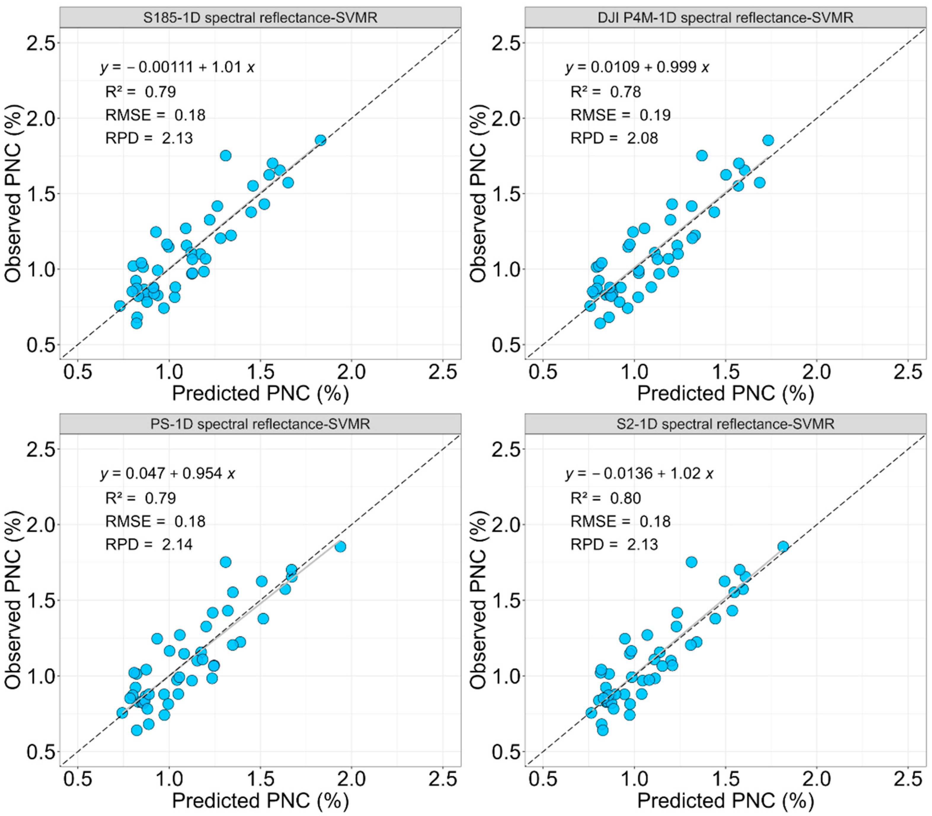
The findings highlighted the predictive capabilities of S185 hyperspectral and simulated (DJI P4M, PS, and S2) sensors for winter wheat PNC. Across all three strategies (1D spectral reflectance, optimized 2D and 3D spectral indices), the S185 hyperspectral sensor consistently demonstrated superior performance in most cases, confirming the value of hyperspectral data for precise PNC evaluation. However, the performance of simulated multispectral UAV and satellite sensors (DJI P4M, PS, and S2) approached that of hyperspectral data when combined with ML models, showcasing their practical application potential. Specifically, the PS based on 1D spectral reflectance strategy combined with SVMR performed the best in PNC prediction (R² = 0.79, RMSE = 0.18, RPD = 2.14), demonstrating a similar accuracy level to the S185 hyperspectral sensor (R² = 0.79, RMSE = 0.18, RPD = 2.13). This shows that, in the case of low spectral dimension, the satellite multispectral sensor could achieve superior prediction accuracy by using appropriate ML models (Figure 5). Gao et al. [43] reached a similar conclusion when predicting the soil aggregates by simulating satellite multispectral bands. The high dimensionality and multicollinearity of the 1D spectral reflectance data from the S185 sensor may have impacted the predictive capability of the PNC model [13].

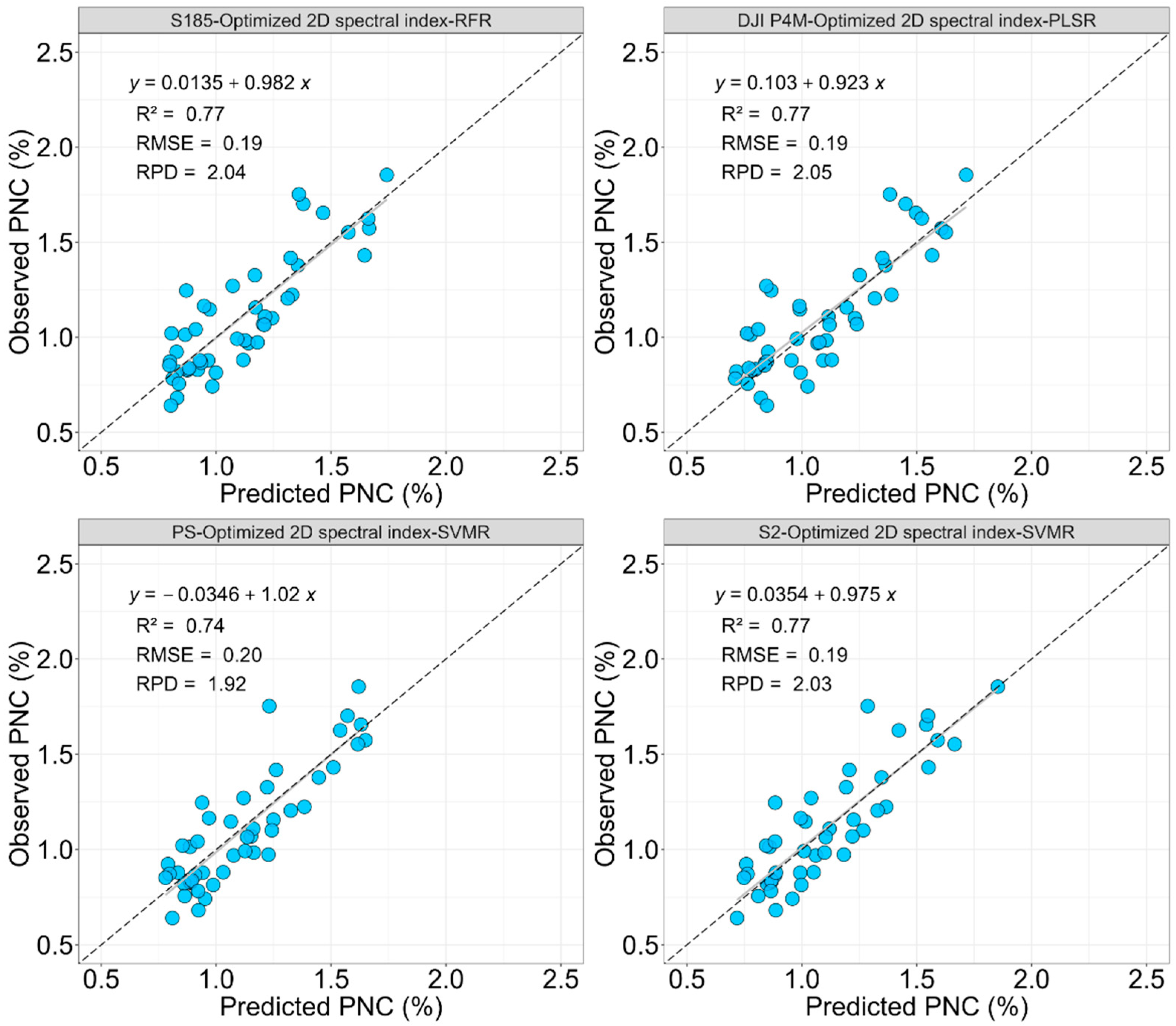
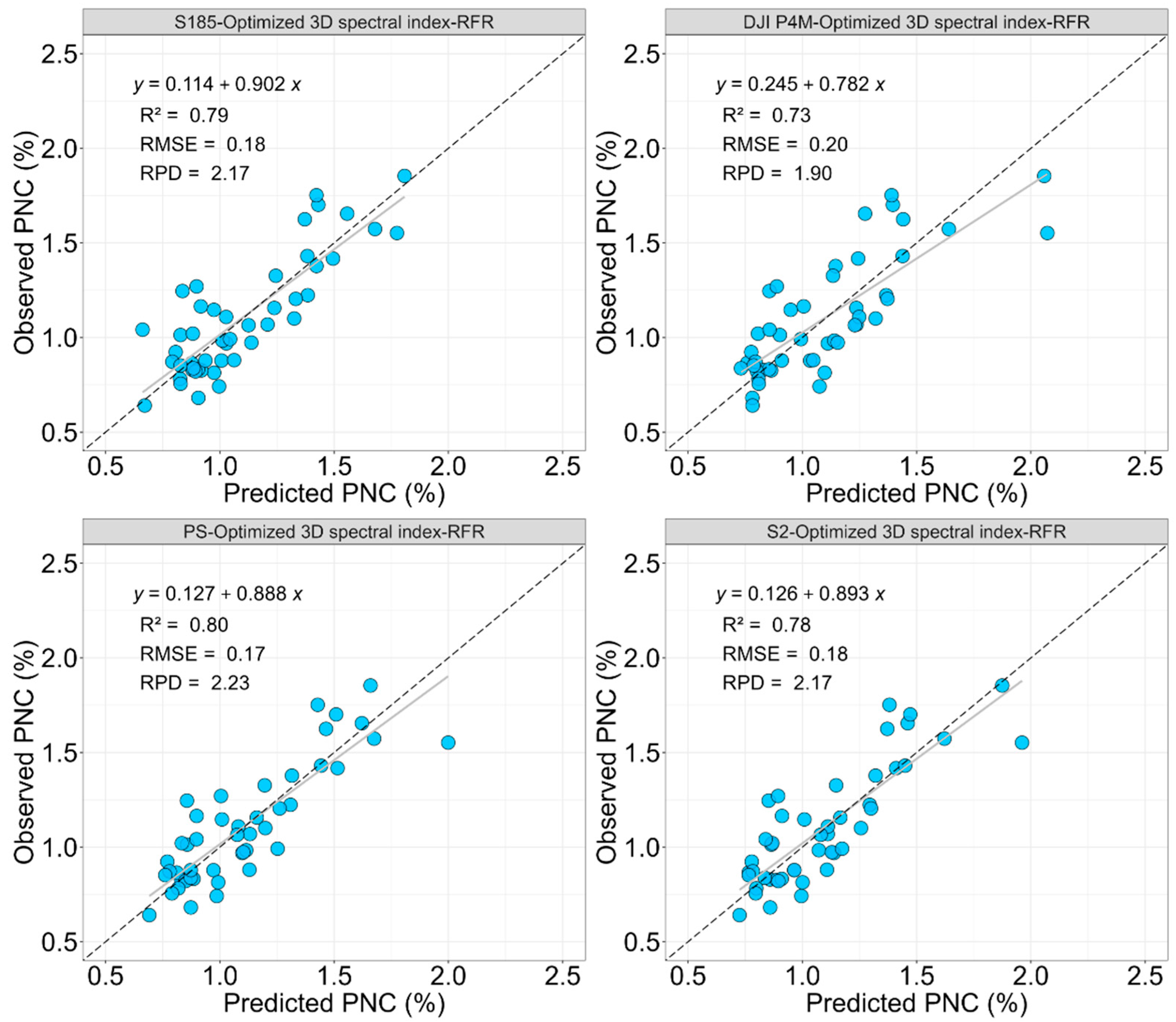
When using optimized 2D spectral indices, model performance varied among sensors too. The S185 hyperspectral sensor achieved the highest accuracy using RFR (R² = 0.77, RMSE = 0.19, RPD = 2.04), while for the simulated DJI P4M and PS sensors, PLSR and SVMR provided the best results, respectively. These findings indicated that spectral indices tailored to specific sensors could compensate for the limited spectral resolution of multispectral sensors, yielding predictive accuracy comparable to hyperspectral data. Notably, the S2 sensor demonstrated good performance with SVMR (R² = 0.77, RMSE = 0.19, RPD = 2.03), further confirming the potential of satellite data combined with optimized indices for PNC monitoring. The use of optimized 3D spectral indices enhanced PNC estimation model accuracy across all sensors. The S185 hyperspectral sensor and the simulated PS sensor showed the best performance with RFR, achieving RPD values of 2.17 and 2.23, respectively. This indicated that incorporating spectral interaction information (3D spectral index) could improve the predictive capabilities of both hyperspectral and multispectral sensors. The S2 sensor also exhibited robust accuracy (R² = 0.78, RMSE = 0.18, RPD = 2.17), further supporting its practical application for large-scale PNC monitoring.

4.2. Comparative Performance of Different ML Models

Compared with PLSR, SVMR and RFR can extract nonlinear features more effectively when processing high-dimensional spectral data in most cases, thus improving the PNC estimation accuracy. SVMR consistently outperformed other ML models when using 1D spectral reflectance, achieving the highest R², lowest RMSE, and highest RPD across most sensors. This demonstrated the robustness of SVMR in capturing complex relationships between spectral reflectance and PNC, even for sensors with fewer spectral bands, such as DJI P4M. However, its relative performance declined with optimized 2D and 3D spectral indices, perhaps because SVMR could fit complex nonlinear relationships in a small sample space and learn the underlying structure of the data while suppressing the influence of noise, allowing it to perform well in the case with limited spectral information [44]. Many previous studies reached similar conclusions [45,46].

RFR exhibited superior performance with optimized 2D and 3D spectral indices, particularly for the S185 and PS sensors. RFR leverages ensemble learning, a strategy that combines predictions from numerous weak learners to produce a more reliable and accurate overall prediction [47]. Each decision tree within the ensemble acts as a weak learner, potentially prone to overfitting on specific data subsets. However, the strength of RFR lies in the amalgamation of these trees, compensating for individual weaknesses and thereby improving the collective predictive capability [48]. Notably, each decision tree in RFR operates as a non-parametric model, effectively capturing irregular data patterns and adapting to intricate relationships. This versatility makes RFR well-suited for managing high-dimensional data and capturing nonlinear relationships [49]. A large part of studies have reached the same conclusion, that RFR is superior to SVMR [6,50]. At present, there is no conclusion on the accuracy of regression prediction between SVMR and RFR.

PLSR, while generally performing worse than SVMR and RFR, demonstrated notable accuracy with optimized 2D spectral indices, particularly for the DJI P4M sensor. Its ability to handle multicollinearity in spectral data makes it a reliable choice for multispectral sensors with fewer bands [51]. However, its lower predictive power with 1D spectral reflectance and optimized 3D spectral indices suggested that its linear modeling approach might struggle with capturing nonlinear patterns in more complex datasets [52]. Overall, these findings emphasized the importance of selecting ML models tailored to the specific characteristics of the input data and sensor type. SVMR and RFR emerged as versatile options for PNC prediction, with RFR particularly excelling in feature-rich datasets.

4.3. Limitations and Research Needs

This research highlights the value of S185 hyperspectral and simulated multispectral sensors for estimating winter wheat PNC. However, there are several limitations to consider. Firstly, although the spectral bands of multispectral sensors (DJI P4M, PS, S2) were simulated, spatial resolution differences were not considered. The higher spatial resolution of S185 hyperspectral sensors captures finer details, whereas coarser-resolution satellite sensors aggregate reflectance over larger areas, potentially impacting model performance and scalability. Specifically, UAV hyperspectral sensors like S185 provide centimeter-level spatial resolution, which enables detection of fine-scale heterogeneity in crop canopies and soil backgrounds. In contrast, satellite sensors such as S2 typically have spatial resolutions of 10 to 20 m, meaning each pixel represents a mixed signal from heterogeneous surfaces. This scale mismatch can reduce the effectiveness of models developed from UAV data when applied to real satellite observations, as satellite data may mask subtle spectral variations important for accurate nitrogen estimation. Furthermore, factors like atmospheric effects, sensor viewing geometry, and temporal revisit frequencies complicate direct translation from UAV simulations to satellite data. Therefore, validating the models with actual satellite imagery is essential.

Secondly, temporal resolution differences were not addressed, although they are critical for operational applications. UAVs allow flexible, on-demand data collection, while satellites like PS offer fixed revisit intervals suitable for crop growth monitoring. S2’s revisit cycle and susceptibility to weather constraints limit temporal consistency.

Moreover, the experiments were conducted on relatively small plots across two site-years, using a single wheat variety and relatively homogeneous soil conditions, limiting the generalizability of findings to broader, more heterogeneous agricultural settings. Finally, the reliance on simulated multispectral data instead of real-world observations underscores the need for further validation with operational UAV and satellite remote sensing systems to assess practical feasibility.

Additionally, while this study focused on optimizing spectral band combinations in index structures, future work should also consider fine-tuning index coefficients to develop more flexible and adaptive vegetation indices for nitrogen estimation.

In summary, this study successfully addressed the initial research objectives by systematically comparing different remote sensing platforms (hyperspectral, UAV multispectral, and satellite multispectral), variable strategies (1D spectral reflectance, optimized 2D and 3D spectral indices), and ML models (PLSR, SVMR, RFR) for estimating winter wheat PNC. The results demonstrate that, with appropriate variable selection and model choice, low-spectral-resolution sensors can approach or even match the performance of hyperspectral data, offering practical value for scalable and cost-effective nitrogen monitoring in precision agriculture. Future research should prioritize addressing spatial and temporal resolution differences, integrating more advanced machine learning and ensemble methods, leveraging multi-source data fusion, validating models across diverse environmental conditions, and developing cross-scale fusion frameworks. These efforts will be essential to fully realize the potential of remote sensing technologies for precision agriculture applications.

5. Conclusions

This study systematically evaluated the prediction accuracy of winter wheat PNC estimation models using S185 hyperspectral and simulated multispectral sensors (DJI P4M, PS, and S2) across three strategies (1D spectral reflectance, optimized 2D and 3D spectral indices). The research results indicated that, for 1D spectral reflectance, SVMR achieved the highest prediction accuracy across all sensors, with R² ranging from 0.78 to 0.80, RMSE of 0.18–0.19%, and RPD of 2.08–2.14. S185 and simulated satellite sensors (PS, S2) outperformed DJI P4M sensor. Under the optimized 2D spectral index strategy, RFR showed the best performance for S185 (R² = 0.77, RMSE = 0.19%, RPD = 2.04), while PLSR and SVMR excelled for DJI P4M and S2 sensor, achieving comparable accuracy (R² = 0.77, RMSE = 0.19%, RPD = 2.03–2.05). For optimized 3D spectral indices, RFR consistently outperformed other models, with PS sensor achieving the highest accuracy (R² = 0.80, RMSE = 0.17%, RPD = 2.23), followed by S185 and S2 (RPD = 2.17). Overall, this study highlighted that, while hyperspectral data provided superior predictive accuracy, the optimized use of multispectral data from PS, S2, and DJI P4M sensors could achieve comparable performance.

Interestingly, the results also suggest that increasing the dimensionality of spectral features (from 1D to 3D) brought only marginal improvements in most cases. In contrast, the selection of an appropriate ML model, particularly RFR and SVMR, had a more significant impact on prediction performance. This finding underscores that, with suitable models, simpler approaches may already deliver robust and scalable solutions for large-scale PNC monitoring. Future research should focus on validating UAV hyperspectral and real satellite remote sensing under diverse field conditions, incorporating advanced ML models and multi-source data fusion to further improve prediction accuracy and operational applicability.

References

1. Yu, Z.; Wang, J.-W.; Chen, L.-P.; Fu, Y.-Y.; Zhu, H.-C.; Feng, H.-K.; Xu, X.-G.; Li, Z.-H. An entirely new approach based on remote sensing data to calculate the nitrogen nutrition index of winter wheat. J. Integr. Agric. 2021, 20, 2535–2551. [Google Scholar] [CrossRef]
2. Huang, S.; Miao, Y.; Yuan, F.; Cao, Q.; Ye, H.; Lenz-Wiedemann, V.I.; Bareth, G. In-season diagnosis of rice nitrogen status using proximal fluorescence canopy sensor at different growth stages. Remote Sens. 2019, 11, 1847. [Google Scholar] [CrossRef]
3. Li, F.; Wang, L.; Liu, J.; Wang, Y.; Chang, Q. Evaluation of leaf N concentration in winter wheat based on discrete wavelet transform analysis. Remote Sens. 2019, 11, 1331. [Google Scholar] [CrossRef]
4. Liang, L.; Di, L.; Zhang, L.; Deng, M.; Qin, Z.; Zhao, S.; Lin, H. Estimation of crop LAI using hyperspectral vegetation indices and a hybrid inversion method. Remote Sens. Environ. 2015, 165, 123–134. [Google Scholar] [CrossRef]
5. Wang, L.; Chang, Q.; Li, F.; Yan, L.; Huang, Y.; Wang, Q.; Luo, L. Effects of growth stage development on paddy rice leaf area index prediction models. Remote Sens. 2019, 11, 361. [Google Scholar] [CrossRef]
6. Kiala, Z.; Odindi, J.; Mutanga, O.; Peerbhay, K. Comparison of partial least squares and support vector regressions for predicting leaf area index on a tropical grassland using hyperspectral data. J. Appl. Remote Sens. 2016, 10, 036015. [Google Scholar] [CrossRef]
7. Yuan, H.; Yang, G.; Li, C.; Wang, Y.; Liu, J.; Yu, H.; Feng, H.; Xu, B.; Zhao, X.; Yang, X. Retrieving soybean leaf area index from unmanned aerial vehicle hyperspectral remote sensing: Analysis of RF, ANN, and SVM regression models. Remote Sens. 2017, 9, 309. [Google Scholar] [CrossRef]
8. Sims, D.A.; Gamon, J.A. Relationships between leaf pigment content and spectral reflectance across a wide range of species, leaf structures and developmental stages. Remote Sens. Environ. 2002, 81, 337–354. [Google Scholar] [CrossRef]
9. Wu, C.; Han, X.; Niu, Z.; Dong, J. An evaluation of EO-1 hyperspectral Hyperion data for chlorophyll content and leaf area index estimation. Int. J. Remote Sens. 2010, 31, 1079–1086. [Google Scholar] [CrossRef]
10. Liang, L.; Qin, Z.; Zhao, S.; Di, L.; Zhang, C.; Deng, M.; Lin, H.; Zhang, L.; Wang, L.; Liu, Z. Estimating crop chlorophyll content with hyperspectral vegetation indices and the hybrid inversion method. Int. J. Remote Sens. 2016, 37, 2923–2949. [Google Scholar] [CrossRef]
11. Xu, M.; Liu, R.; Chen, J.M.; Liu, Y.; Shang, R.; Ju, W.; Wu, C.; Huang, W. Retrieving leaf chlorophyll content using a matrix-based vegetation index combination approach. Remote Sens. Environ. 2019, 224, 60–73. [Google Scholar] [CrossRef]
12. Zhang, J.; Tian, H.; Wang, D.; Li, H.; Mouazen, A.M. A novel approach for estimation of above-ground biomass of sugar beet based on wavelength selection and optimized support vector machine. Remote Sens. 2020, 12, 620. [Google Scholar] [CrossRef]
13. Yue, J.; Zhou, C.; Guo, W.; Feng, H.; Xu, K. Estimation of winter-wheat above-ground biomass using the wavelet analysis of unmanned aerial vehicle-based digital images and hyperspectral crop canopy images. Int. J. Remote Sens. 2021, 42, 1602–1622. [Google Scholar] [CrossRef]
14. Soltanian, M.; Naderi Khorasgani, M.; Tadayyon, A. Estimation of above-ground biomass of winter wheat (Triticum aestivum L.) using multiple linear regression, artificial neural network models remote sensing data. J. Crop Prod. 2020, 13, 179–196. [Google Scholar]
15. Fageria, N.K. The Use of Nutrients in Crop Plants; CRC Press: Boca Raton, FL, USA, 2016. [Google Scholar]
16. Kovács, P.; Vyn, T.J. Relationships between ear-leaf nutrient concentrations at silking and corn biomass and grain yields at maturity. Agron. J. 2017, 109, 2898–2906. [Google Scholar] [CrossRef]
17. Gaju, O.; Allard, V.; Martre, P.; Le Gouis, J.; Moreau, D.; Bogard, M.; Hubbart, S.; Foulkes, M.J. Nitrogen partitioning and remobilization in relation to leaf senescence, grain yield and grain nitrogen concentration in wheat cultivars. Field Crops Res. 2014, 155, 213–223. [Google Scholar] [CrossRef]
18. Li, F.; Miao, Y.; Hennig, S.D.; Gnyp, M.L.; Chen, X.; Jia, L.; Bareth, G. Evaluating hyperspectral vegetation indices for estimating nitrogen concentration of winter wheat at different growth stages. Precis. Agric. 2010, 11, 335–357. [Google Scholar] [CrossRef]
19. Patel, M.K.; Ryu, D.; Western, A.W.; Suter, H.; Young, I.M. Which multispectral indices robustly measure canopy nitrogen across seasons: Lessons from an irrigated pasture crop. Comput. Electron. Agric. 2021, 182, 106000. [Google Scholar] [CrossRef]
20. Dong, R.; Miao, Y.; Wang, X.; Chen, Z.; Yuan, F.; Zhang, W.; Li, H. Estimating plant nitrogen concentration of maize using a leaf fluorescence sensor across growth stages. Remote Sens. 2020, 12, 1139. [Google Scholar] [CrossRef]
21. Yu, K.; Li, F.; Gnyp, M.L.; Miao, Y.; Bareth, G.; Chen, X. Remotely detecting canopy nitrogen concentration and uptake of paddy rice in the Northeast China Plain. ISPRS J. Photogramm. Remote Sens. 2013, 78, 102–115. [Google Scholar] [CrossRef]
22. Chen, P.; Haboudane, D.; Tremblay, N.; Wang, J.; Vigneault, P.; Li, B. New spectral indicator assessing the efficiency of crop nitrogen treatment in corn and wheat. Remote Sens. Environ. 2010, 114, 1987–1997. [Google Scholar] [CrossRef]
23. Stroppiana, D.; Boschetti, M.; Brivio, P.A.; Bocchi, S. Plant nitrogen concentration in paddy rice from field canopy hyperspectral radiometry. Field Crops Res. 2009, 111, 119–129. [Google Scholar] [CrossRef]
24. Wang, L.; Chen, S.; Li, D.; Wang, C.; Jiang, H.; Zheng, Q.; Peng, Z. Estimation of paddy rice nitrogen content and accumulation both at leaf and plant levels from UAV hyperspectral imagery. Remote Sens. 2021, 13, 2956. [Google Scholar] [CrossRef]
25. Yao, X.; Huang, Y.; Shang, G.; Zhou, C.; Cheng, T.; Tian, Y.; Cao, W.; Zhu, Y. Evaluation of six algorithms to monitor wheat leaf nitrogen concentration. Remote Sens. 2015, 7, 14939–14966. [Google Scholar] [CrossRef]
26. Wang, H.-F.; Huo, Z.-G.; Zhou, G.-S.; Liao, Q.-H.; Feng, H.-K.; Wu, L. Estimating leaf SPAD values of freeze-damaged winter wheat using continuous wavelet analysis. Plant Physiol. Biochem. 2016, 98, 39–45. [Google Scholar] [CrossRef]
27. Bruce, L.M.; Koger, C.H.; Li, J. Dimensionality reduction of hyperspectral data using discrete wavelet transform feature extraction. IEEE Trans. Geosci. Remote Sens. 2002, 40, 2331–2338. [Google Scholar] [CrossRef]
28. Blackburn, G.A.; Ferwerda, J.G. Retrieval of chlorophyll concentration from leaf reflectance spectra using wavelet analysis. Remote Sens. Environ. 2008, 112, 1614–1632. [Google Scholar] [CrossRef]
29. Chen, J.; Li, F.; Wang, R.; Fan, Y.; Raza, M.A.; Liu, Q.; Wang, Z.; Cheng, Y.; Wu, X.; Yang, F. Estimation of nitrogen and carbon content from soybean leaf reflectance spectra using wavelet analysis under shade stress. Comput. Electron. Agric. 2019, 156, 482–489. [Google Scholar] [CrossRef]
30. Cheng, T.; Rivard, B.; Sanchez-Azofeifa, A. Spectroscopic determination of leaf water content using continuous wavelet analysis. Remote Sens. Environ. 2011, 115, 659–670. [Google Scholar] [CrossRef]
31. Zhang, J.; Pu, R.; Loraamm, R.W.; Yang, G.; Wang, J. Comparison between wavelet spectral features and conventional spectral features in detecting yellow rust for winter wheat. Comput. Electron. Agric. 2014, 100, 79–87. [Google Scholar] [CrossRef]
32. Liao, Q.; Wang, J.; Yang, G.; Zhang, D.; Lii, H.; Fu, Y.; Li, Z. Comparison of spectral indices and wavelet transform for estimating chlorophyll content of maize from hyperspectral reflectance. J. Appl. Remote Sens. 2013, 7, 073575. [Google Scholar] [CrossRef]
33. Li, L.; Geng, S.; Lin, D.; Su, G.; Zhang, Y.; Chang, L.; Ji, Y.; Wang, Y.; Wang, L. Accurate modeling of vertical leaf nitrogen distribution in summer maize using in situ leaf spectroscopy via CWT and PLS-based approaches. Eur. J. Agron. 2022, 140, 126607. [Google Scholar] [CrossRef]
34. Wang, Z.; Chen, J.; Zhang, J.; Tan, X.; Raza, M.A.; Ma, J.; Zhu, Y.; Yang, F.; Yang, W. Assessing canopy nitrogen and carbon content in maize by canopy spectral reflectance and uninformative variable elimination. Crop J. 2022, 10, 1224–1238. [Google Scholar] [CrossRef]
35. Liu, N.; Xing, Z.; Zhao, R.; Qiao, L.; Li, M.; Liu, G.; Sun, H. Analysis of Chlorophyll Concentration in Potato Crop by Coupling Continuous Wavelet Transform and Spectral Variable Optimization. Remote Sens. 2020, 12, 2826. [Google Scholar] [CrossRef]
36. Bangalore, A.S.; Shaffer, R.E.; Small, G.W.; Arnold, M.A. Genetic algorithm-based method for selecting wavelengths and model size for use with partial least-squares regression: Application to near-infrared spectroscopy. Anal. Chem. 1996, 68, 4200–4212. [Google Scholar] [CrossRef]
37. Galvao, R.K.H.; Araujo, M.C.U.; Fragoso, W.D.; Silva, E.C.; Jose, G.E.; Soares, S.F.C.; Paiva, H.M. A variable elimination method to improve the parsimony of MLR models using the successive projections algorithm. Chemom. Intell. Lab. Syst. 2008, 92, 83–91. [Google Scholar] [CrossRef]
38. Li, H.; Liang, Y.; Xu, Q.; Cao, D. Key wavelengths screening using competitive adaptive reweighted sampling method for multivariate calibration. Anal. Chim. Acta 2009, 648, 77–84. [Google Scholar] [CrossRef] [PubMed]
39. Fan, L.; Zhao, J.; Xu, X.; Liang, D.; Yang, G.; Feng, H.; Yang, H.; Wang, Y.; Chen, G.; Wei, P. Hyperspectral-based estimation of leaf nitrogen content in corn using optimal selection of multiple spectral variables. Sensors 2019, 19, 2898. [Google Scholar] [CrossRef]
40. Bai, L.-M.; Li, F.-L.; Chang, Q.-R.; Zeng, F.; Cao, J.; Lu, G. Increasing accuracy of hyper· spectral remote sensing for total nitrogen of winter wheat canopy by use of SPA and PLS methods. J. Plant. Nutr. Fertil 2018, 24, 52–58. [Google Scholar]
41. Ollinger, S.V. Sources of variability in canopy reflectance and the convergent properties of plants. New Phytol. 2011, 189, 375–394. [Google Scholar] [CrossRef]
42. Luo, J.; Ying, K.; He, P.; Bai, J. Properties of Savitzky–Golay digital differentiators. Digit. Signal Process. 2005, 15, 122–136. [Google Scholar] [CrossRef]
43. Liao, Q.; Gu, X.; Li, C.; Chen, L.; Huang, W.; Du, S.; Fu, Y.; Wang, J. Estimation of fluvo-aquic soil organic matter content from hyperspectral reflectance based on continuous wavelet transformation. Trans. Chin. Soc. Agric. Eng. 2012, 28, 132–139. [Google Scholar]
44. Araújo, M.C.U.; Saldanha, T.C.B.; Galvao, R.K.H.; Yoneyama, T.; Chame, H.C.; Visani, V. The successive projections algorithm for variable selection in spectroscopic multicomponent analysis. Chemom. Intell. Lab. Syst. 2001, 57, 65–73. [Google Scholar] [CrossRef]
45. Wold, S.; Sjöström, M.; Eriksson, L. PLS-regression: A basic tool of chemometrics. Chemom. Intell. Lab. Syst. 2001, 58, 109–130. [Google Scholar] [CrossRef]
46. Nigon, T.J.; Yang, C.; Dias Paiao, G.; Mulla, D.J.; Knight, J.F.; Fernández, F.G. Prediction of Early Season Nitrogen Uptake in Maize Using High-Resolution Aerial Hyperspectral Imagery. Remote Sens. 2020, 12, 1234. [Google Scholar] [CrossRef]
47. Chauchard, F.; Cogdill, R.; Roussel, S.; Roger, J.; Bellon-Maurel, V. Application of LS-SVM to non-linear phenomena in NIR spectroscopy: Development of a robust and portable sensor for acidity prediction in grapes. Chemom. Intell. Lab. Syst. 2004, 71, 141–150. [Google Scholar] [CrossRef]
48. Singh, K.P.; Malik, A.; Basant, N.; Saxena, P. Multi-way partial least squares modeling of water quality data. Anal. Chim. Acta 2007, 584, 385–396. [Google Scholar] [CrossRef] [PubMed]
49. Li, C.; Wang, Y.; Ma, C.; Ding, F.; Li, Y.; Chen, W.; Li, J.; Xiao, Z. Hyperspectral estimation of winter wheat leaf area index based on continuous wavelet transform and fractional order differentiation. Sensors 2021, 21, 8497. [Google Scholar] [CrossRef]
50. Zhao, R.; An, L.; Song, D.; Li, M.; Qiao, L.; Liu, N.; Sun, H. Detection of chlorophyll fluorescence parameters of potato leaves based on continuous wavelet transform and spectral analysis. Spectrochim. Acta Part A Mol. Biomol. Spectrosc. 2021, 259, 119768. [Google Scholar] [CrossRef]
51. Yao, Q.; Zhang, Z.; Lv, X.; Chen, X.; Ma, L.; Sun, C. Estimation Model of Potassium Content in Cotton Leaves Based on Wavelet Decomposition Spectra and Image Combination Features. Front. Plant Sci. 2022, 13, 920532. [Google Scholar] [CrossRef]
52. Wang, Z.; Chen, J.; Fan, Y.; Cheng, Y.; Wu, X.; Zhang, J.; Wang, B.; Wang, X.; Yong, T.; Liu, W. Evaluating photosynthetic pigment contents of maize using UVE-PLS based on continuous wavelet transform. Comput. Electron. Agric. 2020, 169, 105160. [Google Scholar] [CrossRef]
Figure 1. Location and outline of the field experiments.
Remotesensing 17 02666 g001
Figure 2. The workflow for estimating winter wheat PNC.
Remotesensing 17 02666 g002
Figure 3. Correlation heat maps between PNC and 2D spectral indices from the S185 sensor. Each subplot’s color bar on the right displayed the correlation (R) values. The wavelengths at 450–950 nm were represented by the x- and y-, z-axes.
Remotesensing 17 02666 g003
Figure 4. Correlation horizontal slice diagrams between PNC and 3D spectral indices from the S185 sensor. Each subplot’s color bar on the right displayed the correlation (R) values. The wavelengths at 450–950 nm were represented by the x-, y-, and z-axes.
Remotesensing 17 02666 g004
Figure 5. Scatter plots of observed vs. predicted PNC (%) for the best models based on 1D spectral reflectance derived from different sensors. The gray line indicates the regression fit, and the dashed line denotes the 1:1 line.
Remotesensing 17 02666 g005
Figure 6. Scatter plots of observed vs. predicted PNC (%) for the best models using optimized 2D spectral indices derived from different sensors. The gray line indicates the regression fit, and the dashed line denotes the 1:1 line.
Remotesensing 17 02666 g006
Figure 7. Scatter plots of observed vs. predicted PNC (%) for the best models based on optimized 3D spectral indices derived from different sensors. The gray line indicates the regression fit, and the dashed line denotes the 1:1 line.
Remotesensing 17 02666 g007