Article

The Downscaled GOME-2 SIF Based on Machine Learning Enhances the Correlation with Ecosystem Productivity

1
School of Environmental Science and Optoelectronic Technology, University of Science and Technology of China, Hefei 230026, China
2
Key Laboratory of Environmental Optical and Technology, Anhui Institute of Optics and Fine Mechanics, Hefei Institutes of Physical Science, Chinese Academy of Sciences, Hefei 230031, China
3
Institute of Environment, Hefei Comprehensive National Science Center, Hefei 230031, China
4
College of Resources and Environment, University of Chinese Academy of Sciences, Beijing 101408, China
*
Author to whom correspondence should be addressed.
Remote Sens. 2025, 17(15), 2642; https://doi.org/10.3390/rs17152642
Submission received: 5 June 2025 / Revised: 25 July 2025 / Accepted: 28 July 2025 / Published: 30 July 2025

Abstract

Sun-induced chlorophyll fluorescence (SIF) is an important indicator of vegetation photosynthesis. While remote sensing enables large-scale monitoring of SIF, existing products face the challenge of trade-offs between temporal and spatial resolutions, limiting their applications. To select the optimal model for SIF data downscaling, we used a consistent dataset combined with vegetation physiological and meteorological parameters to evaluate four different regression methods in this study. The XGBoost model demonstrated the best performance during cross-validation (R2 = 0.84, RMSE = 0.137 mW/m2/nm/sr) and was, therefore, selected to downscale GOME-2 SIF data. The resulting high-resolution SIF product (HRSIF) has a temporal resolution of 8 days and a spatial resolution of 0.05° × 0.05°. The downscaled product shows high fidelity to the original coarse SIF data when aggregated (correlation = 0.76). The reliability of the product was ensured through cross-validation with ground-based and satellite observations. Moreover, the finer spatial resolution of HRSIF better matches the footprint of eddy covariance flux towers, leading to a significant improvement in the correlation with tower-based gross primary productivity (GPP). Specifically, in the mixed forest vegetation type with the best performance, the R2 increased from 0.66 to 0.85, representing an increase of 28%. This higher-precision product will support more effective ecosystem monitoring and research.

1. Introduction

Due to the close association with photosynthesis, chlorophyll fluorescence has become an important indicator for characterizing terrestrial photosynthesis and is widely used in fields of ecosystem carbon cycling, vegetation drought stress monitoring, and pest and disease detection [1,2,3]. In recent years, several studies have evaluated satellite-derived SIF signals, mainly from satellites that cover the SIF emission bands, such as GOSAT, OCO-2, TanSat, and TROPOMI [4,5,6]. Satellite SIF signals have shown strong correlations with the gross primary productivity (GPP) of terrestrial ecosystems at both global and regional scales [7,8]. However, the early launched instruments, such as GOSAT and GOME-2, had relatively low spatial and temporal resolutions, which were insufficient for ecosystem monitoring requirements. Although the new instruments on satellites, such as OCO-2 and TROPOMI, provide high spatial resolution (covering an area of several kilometers), they still have some limitations in terms of spatial sampling and archival time. Therefore, in order to provide SIF data products with high resolution, spatial continuity, and high temporal frequency, it is necessary to reconfigure them.
Reconstruction studies of different satellite products primarily focus on two aspects. The first is spatial reconstruction, which targets satellite products with very coarse spatial resolution, such as SCIAMACHY and GOME-2, whose spatial resolution is on the order of tens of kilometers. Spatial downscaling enhances the spatial detail of these products, allowing for better alignment with ecosystem flux observations [9,10]. In recent years, with the continuous improvement of satellite spatial resolution, spatial reconstruction products for high-resolution datasets have also emerged, such as the TroDSIF product developed by Liu Liangyun’s team, which is a new SIF product with a spatial resolution of 500 m generated from the original 0.05° TROPOMI SIF [11]. The second is temporal reconstruction. Recently launched satellites like TROPOMI offer high spatial resolution and wide coverage but have relatively short data records, limiting the application. By developing SIF prediction models, it is possible to estimate historical SIF values and generate high-precision data products beyond the satellite’s operational lifespan, which is highly beneficial for studying long-term ecosystem changes [12]. For example, Li Xing’s team’s GOSIF project performed temporal reconstruction on raw OCO-2 SIF data, extending its archival range back to the year 2000 [13].
In terms of data reconstruction methods, the main approach is to establish the relationship between SIF and its related explanatory variables, using either physical models or machine learning techniques. Physically based methods are typically built on the concept of light use efficiency to develop nonlinear models relating SIF to relevant variables. For example, Duveiller et al. constructed a nonlinear model to characterize SIF using NDVI, ET, and LST [14]. These methods can intuitively illustrate the relationships between variables and SIF but require highly accurate input data. A growing number of studies have adopted machine learning approaches [15,16], as they allow the incorporation of more variables and better capture complex nonlinear relationships among them. Machine learning has been widely applied in the downscaling of satellite data, with various studies using it to enhance the spatiotemporal resolution of satellite products [17,18]. Each machine learning method has its strengths and weaknesses and may vary in suitability depending on the spatial scale. At the global scale, tree-based models are often adopted due to their high computational efficiency and robust predictive accuracy when handling large-scale aggregated data [19,20]. In contrast, regional-scale studies typically focus on using higher-resolution data to capture more complex nonlinear relationships. In this context, the architectural flexibility of neural networks offers a clear advantage in modelling these complex patterns, despite their higher computational demands, as they may yield higher accuracy [21,22]. Balancing training efficiency and prediction accuracy is key when selecting an appropriate machine learning algorithm. Meanwhile, unlike traditional statistical models, machine learning models are often considered “black boxes” that do not provide clear interpretations of variable relationships, making the interpretability of machine learning models an important consideration.
Currently, multiple ground-based SIF observation systems have been established for different vegetation communities, providing continuous real-time SIF observations [23]. This is also an important validation method for original satellite data and downscaled products. However, the time-reconstruction products mentioned above cannot be validated against original data outside the satellite data record, making spatial downscaling of long-term satellite products still highly valuable. For global-scale SIF product downscaling, machine learning methods are more efficient, and model interpretability can be enhanced using SHAP analysis. Comparing different algorithms to select the most suitable one for the target data is also a key focus of research.
Therefore, this study is based on the GOME-2 SIF product and adopts a two-step downscaling framework. First, a model is constructed to represent the relationship between the explanatory variables and the SIF at a resolution of 0.5°. Then, this model is applied at a resolution of 0.05°. By comparing models, we selected the most suitable machine learning algorithm and achieved the following: (a) Using reflectance, NDVI, land surface temperature, MODIS photosynthetically active radiation, and land cover type data, the original 0.5° SIF data were improved to a resolution of 0.05°. The resulting product outperforms the original in spatial coverage and detail while preserving the original SIF’s spatiotemporal characteristics. (b) The results of this study were compared with ground-based SIF observations and other satellite SIF products, validating the feasibility and accuracy of the proposed approach. (c) Correlation analysis between the improved product and GPP data from FluxNET eddy covariance towers showed that the downscaled product had an improved correlation with GPP. Additionally, we quantified the contribution of different feature parameters to the model’s predictions and emphasized the influence of categorical variables—particularly land cover data—on model performance.

2. Materials and Methods

2.1. Materials

2.1.1. Explanatory Variable

Explanatory variables are the parameters used to scale down the SIF data and are the input features of the model. Based on the light energy utilization model of GPP [16], a similar SIF formula can be obtained:
S I F = S I F y i e l d · A P A R = F · f e s c · P A R · f P A R
where S I F y i e l d is the amount of fluorescence emitted per unit photon absorbed, generally expressed as the product of fluorescence quantum yield F and fluorescence escape probability fesc; P A R denotes the photosynthetically active radiation, i.e., the portion of sunlight that can be absorbed by vegetation, which is usually between 400 and 800 nm; f P A R is the proportion of photosynthetically active radiation absorbed by the vegetation, which is related to the nature of the vegetation itself; their product is expressed as APAR, the absorbed photosynthetically active radiation.
This physical relationship forms the theoretical basis for selecting explanatory variables in the downscaling model. Our goal is to use machine learning algorithms to build predictive models from these driving factors to reconstruct high-resolution SIF. Since specific values such as fluorescence quantum yield are generally difficult to measure at the satellite scale, this study, based on the above principles, selects typical factors influencing vegetation photosynthesis as explanatory variables. These variables are categorized into three groups based on their source of influence: vegetation variables, meteorological variables, and land use/land cover type variables. Vegetation variables reflect the growth status of vegetation, such as vegetation indices and reflectance. Meteorological variables represent the environmental conditions for vegetation growth and are key factors affecting vegetation dynamics, including temperature and radiation. Land use types, as categorical variables, represent different vegetation types. Studies have shown that different vegetation types exhibit different levels of SIF intensity [4].
The dataset of explanatory variables used in this study includes reflectance, normalized difference vegetation index (NDVI), land surface temperature (LST), photosynthetically active radiation (PAR), and land use/land cover (LULC). Reflectance, NDVI, LST, and LULC data were obtained from MODIS sensors aboard the Terra and Aqua satellites, which provide extensive information on land surface characteristics. We selected the MCD43C4 daily nadir BRDF-adjusted reflectance product [24], which offers 0.05° daily reflectance data across 7 spectral bands. NDVI was calculated using the red and near-infrared bands. LST data were derived from the MOD11C1 product [25], which provides 0.05° daily land surface temperature data. Land cover data were obtained from the MCD12C1 product [26], which provides land cover classification at 0.05° resolution and includes three classification schemes. This study adopted the IGBP classification scheme, which includes 17 land cover types, as shown in the caption of Figure 1. Since this data are discrete categorical data, we employed a one-hot encoder to convert them from a categorical form to a numerical form, aligning with the input data type recognizable by machine learning algorithms. PAR represents the portion of light that is effective for vegetation photosynthesis. PAR data were downloaded from the Clouds and Earth’s Radiant Energy System (CERES) SYN1deg global PAR product [27], which has a spatial resolution of 1° × 1° and a daily temporal resolution. This dataset includes both direct and diffuse radiation under all-sky and clear-sky conditions, with total PAR calculated as the sum of all-sky direct and diffuse components.

2.1.2. GOME-2 SIF Data

GOME-2 is a scanning spectrometer carried aboard the MetOp series of polar-orbiting satellites, which was designed for monitoring atmospheric ozone and other trace gases. It was launched in October 2006 and has been in operation since early 2007, accumulating more than a decade of observational data. Due to its spectral coverage extending into the near-infrared region (around 740 nm), it has also been used for retrieving SIF data [28]. Before 2013, its observational footprint was 40 × 80 km, which was improved to 40 × 40 km after 2013, with a revisit time of approximately 1.5 days. Using a data-driven approach, P. Köhler et al. retrieved GOME-2 SIF data at 740 nm and compiled them into a daily observation dataset spanning 2007–2018 with a spatial resolution of 0.5° × 0.5°. The GOME-2 SIF product provides relatively high temporal resolution, making it valuable for studying long-term ecosystem changes. However, its coarse spatial resolution limits its range of applications. Therefore, to enhance its usability and value, it is necessary to improve its spatial resolution. Since GOME-2 collects spectral data at approximately 9:30 a.m. daily, a correction factor must be applied to convert instantaneous observations into daily values. To ensure input data quality, only observations with a cloud fraction of less than 50% were retained through a quality control process [29]. The data used to construct the model are listed in Table 1.

2.1.3. Validation Data

Satellite-based SIF observations represent a regional and large-scale remote sensing method. Therefore, to verify the accuracy of these data, it is essential to perform cross-comparisons using in situ near-surface observations. In recent years, several ground-based SIF observation systems have been developed to meet the requirements of ecosystem and canopy-scale monitoring [30,31]. One such system is PhotoSpec, a ground-based spectrometer system designed to measure SIF distributions in the red (670–732 nm) and far-red (729–784 nm) wavelength ranges [30]. The system is usually mounted on a flux tower, and its height from the underlying surface is determined based on the observed target. Continuous measurements are usually conducted during the day, and the data are processed to a 30 min time resolution to match the results of flux measurements. According to observational data provided by Pierrat et al., measurements were conducted at two sites: CA-OBS in Canada (53.98°N, 105.12°W) and US-NR1 in Colorado, USA (40.03°N, 105.55°W) [32,33]. On the other hand, the China Spectral Observation Network provides continuous SIF monitoring at multiple flux tower sites across China [23], offering standard 30 min and daily average observations. Two sites, Huailai in Hebei Province and Jurong in Jiangsu Province, were selected from publicly available datasets for validation purposes [31,34]. During the site selection process, we excluded locations with insufficient observation periods or poor data quality. Ultimately, only the above four sites were retained, as their reliability had been utilized and verified in previous studies.
Additionally, we conducted comparative analyses with existing satellite SIF products, including the TROPOMI SIF product and the GOME-2 0.05° product. The TROPOMI SIF dataset used is the gridded 0.05° × 0.05° eSIF product, which is an 8-day composite derived from “baseline” SIF retrievals in the 743–758 nm band. The dataset excludes observations with a cloud fraction > 0.2, a viewing zenith angle > 0.5, or with invalid cloud screening [35]. The GOME-2 SIF product referenced here, known as SIFDuveiller, was developed by Duveiller et al. using GOME-2 SIF data downscaled via a Light Use Efficiency (LUE) model to 8-day, 0.05° × 0.05° resolution [36].

2.2. Method

2.2.1. Selection of Downscaling Algorithm

Extreme Gradient Boosting (XGBoost) is an algorithm based on Gradient-Boosted Decision Trees (GBDT) [37]. While sharing the core concept of GBDT, XGBoost incorporates a number of optimizations, making it particularly well-suited for large-scale datasets and high-dimensional features. It is a tree-based ensemble learning algorithm that enhances model performance by optimizing tree structure and node splitting. As a boosting algorithm, XGBoost iteratively builds models, where each iteration re-weights the samples based on the prediction errors from the previous iteration. With each iteration, the residual error decreases, reducing model bias and effectively preventing overfitting. Tree-based models have been widely used in various remote sensing regression tasks, including the spatial downscaling of SIF data [9,38]. Therefore, in this study, the XGBoost regression model was employed to perform spatial downscaling on the sparsely distributed GOME-2 SIF products.
To evaluate the performance of the XGBoost model, we also introduced Multivariate Linear Regression (MLR), Random Forest (RF), and MLPRegressor (multilayer perceptron Regressor) as comparative models during training. The accuracy of these regression models reflects the degree to which the selected explanatory variables explain the sample variance, and can be evaluated using metrics such as Root Mean Square Error (RMSE), Mean Absolute Error (MAE), and the coefficient of determination (R2), with their formulas defined as follows:
R M S E = 1 n i = 1 n y i ^ y i 2
M A E = 1 n i = 1 n y i ^ y i
R 2 = 1 i = 1 n y i ^ y i 2 i = 1 n y i ^ y i ¯ 2
where y i ^ represents the SIF predicted value, y i represents the SIF true value, y i ¯ is the sample mean, and n is the sample size.

2.2.2. Downscaling Process and Data Preprocessing

This study adopts a two-step downscaling approach to generate high-resolution SIF data using a downscaling model. First, at a coarse spatial resolution of 0.5°, the GOME-2 SIF data are linked with explanatory variables to establish a predictive model. These explanatory variables include reflectance, photosynthetically active radiation (PAR), and other meteorological and vegetation parameters. The study uses data from the entire year of 2007–2008 as the sample, with two-thirds used as the training set and one-third as the validation set. Second, once the model is trained, higher-resolution (0.05°) explanatory variables are input to predict and generate SIF data at a 0.05° resolution.
During the model construction process, all input explanatory variables are first resampled to ensure spatial consistency with the coarse 0.5° resolution of the GOME-2 SIF. In addition, a quality control procedure is applied to filter out low-quality observations and eliminate cloud contamination. A Savitzky–Golay (SG) filter is used to fill spatial gaps left by cloud removal [19]. The objective of this study is to create a high spatiotemporal resolution SIF dataset with a spatial resolution of 0.05° and a temporal frequency of 8 days. The daily SIF predictions were aggregated into an 8-day resolution, primarily to generate complete spatial maps by mitigating the impact of clouds on the data and to improve the signal-to-noise ratio. To achieve this, an additional temporal aggregation step is performed to summarize daily data into 8-day averages. The full processing workflow is illustrated in Figure 2.

3. Results

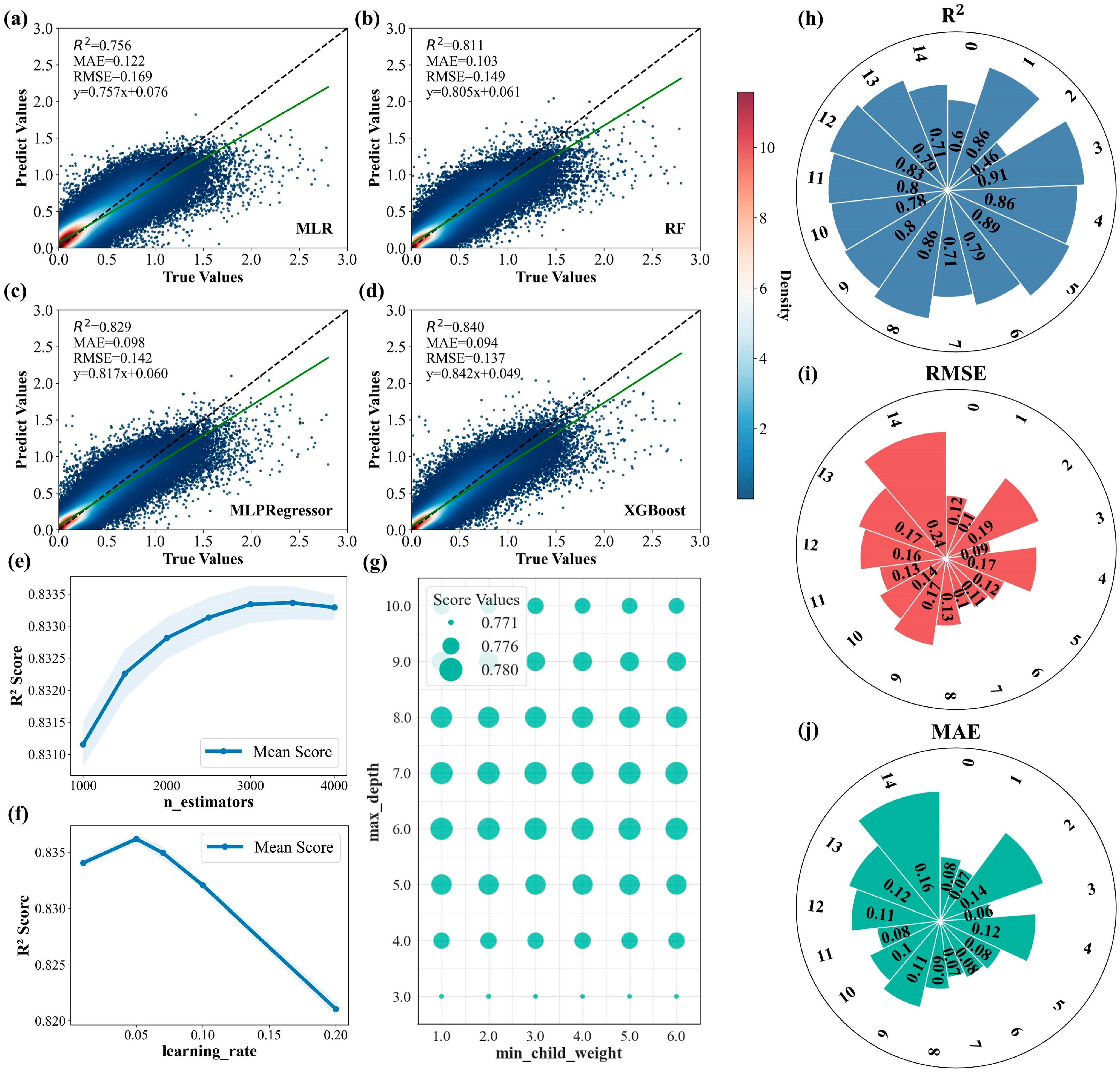
3.1. Model Comparison and Accuracy Evaluation

Based on the same set of sample data, we compared the performance of four different models—MLR, RF, MLPRegressor, and XGBoost—during the training process. Comparative analysis using multiple evaluation metrics showed that the XGBoost model demonstrated superior predictive performance. In terms of model evaluation, XGBoost achieved the lowest MAE and RMSE while having an R2 value closest to the theoretical optimum of one, as shown in Figure 3a–d, indicating its excellent prediction accuracy and stability. The comparison results suggest that, for the global GOME-2 SIF data, XGBoost outperforms the commonly used RF algorithm in terms of accuracy. Although MLPRegressor achieves comparable prediction results to XGBoost, it requires significantly longer training time.
When building the model using the XGBoost algorithm, hyperparameter tuning is typically required before model fitting to avoid issues such as overfitting. Grid search provides a list of values for each specified hyperparameter to be optimized and tests all possible combinations of these values [39]. This method is characterized by exhaustive exploration of parameter combinations. If the step size is small enough and the parameter range is wide, the model can theoretically approach the global optimum. However, due to the enormous computational load, this process is very slow. Therefore, this study adopted a hybrid approach combining manual tuning and grid search to optimize parameters. One hyperparameter was optimized at a time, using the best-fitting result from the previous step to guide the tuning of the next. The hyperparameters were tuned sequentially in the following order: n_estimators, min_child_weight, max_depth, and learning_rate. Final values were selected based on the best-fitting results. The impact of each hyperparameter on training performance is shown in Figure 3e–g). For each parameter, training metrics reached a peak before declining; the peak was selected as the optimal hyperparameter value. The final list of optimal hyperparameters is shown in Table 2.
In addition to evaluating the overall performance of the model at the global scale, we further assessed its testing performance across different ecosystems based on land cover classification data to verify regional robustness. The results showed that the model exhibited strong predictive accuracy across all ecosystem types, as shown in Figure 3h–j. The land cover categories corresponding to the classification codes are listed in the caption of Figure 1. Among them, the model performed best in forest ecosystems, while performance in water bodies and open shrublands was relatively lower. This discrepancy may be attributed to the high spatial heterogeneity in sparsely vegetated areas, which increases intra-pixel noise and reduces model stability. Notably, the model performed poorly in evergreen broadleaf forests (IGBP = 2), where the R2 value was relatively low. This finding is consistent with the results reported by Li et al. [40]. As shown in the global land cover map (Figure 1), this vegetation type is mainly distributed in tropical rainforest regions such as the Amazon. These areas are frequently affected by cloud cover, resulting in higher noise levels in remote sensing data [41]. In addition, the subtle seasonal changes in the canopy structure of evergreen broadleaf forests make it difficult for moderate-resolution sensors (e.g., MODIS) to detect fine spectral differences, which in turn affects model accuracy [42].

3.2. Verification of HRSIF

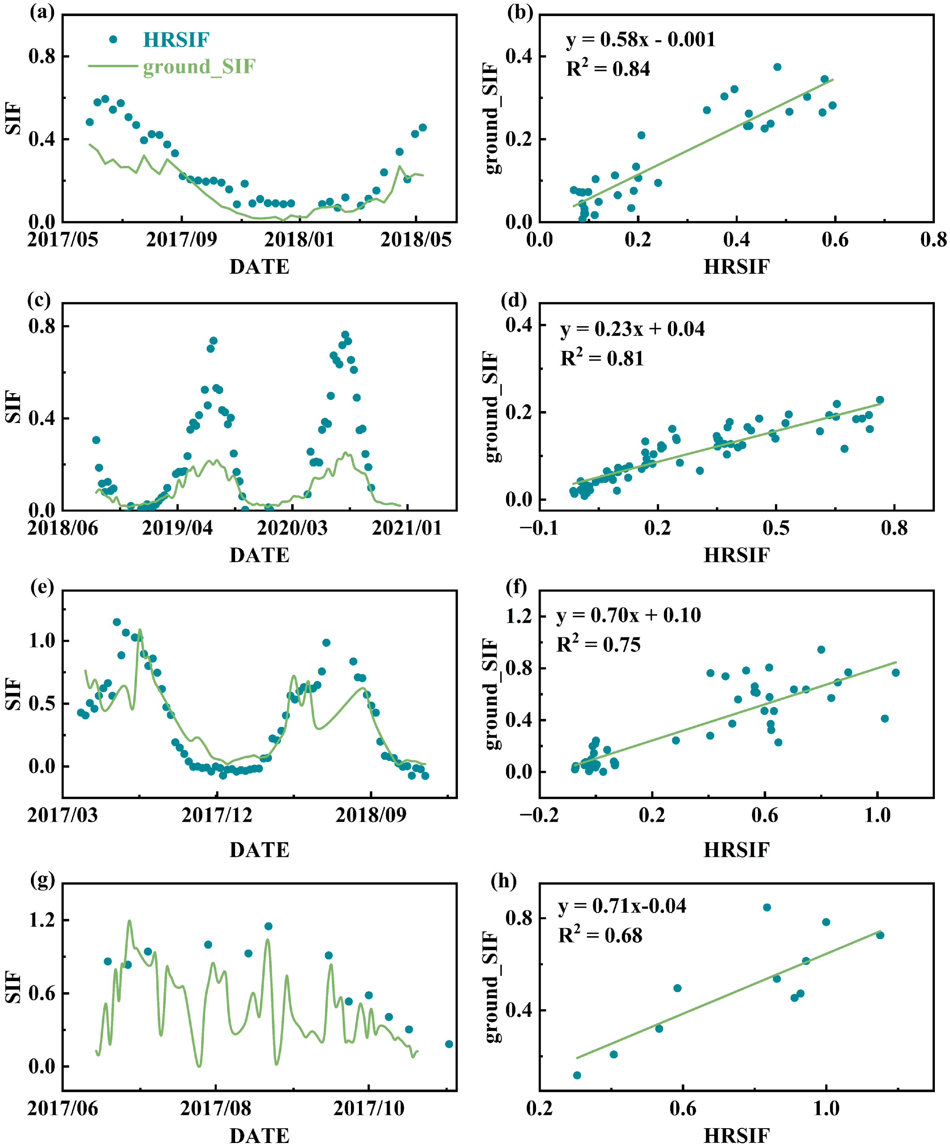
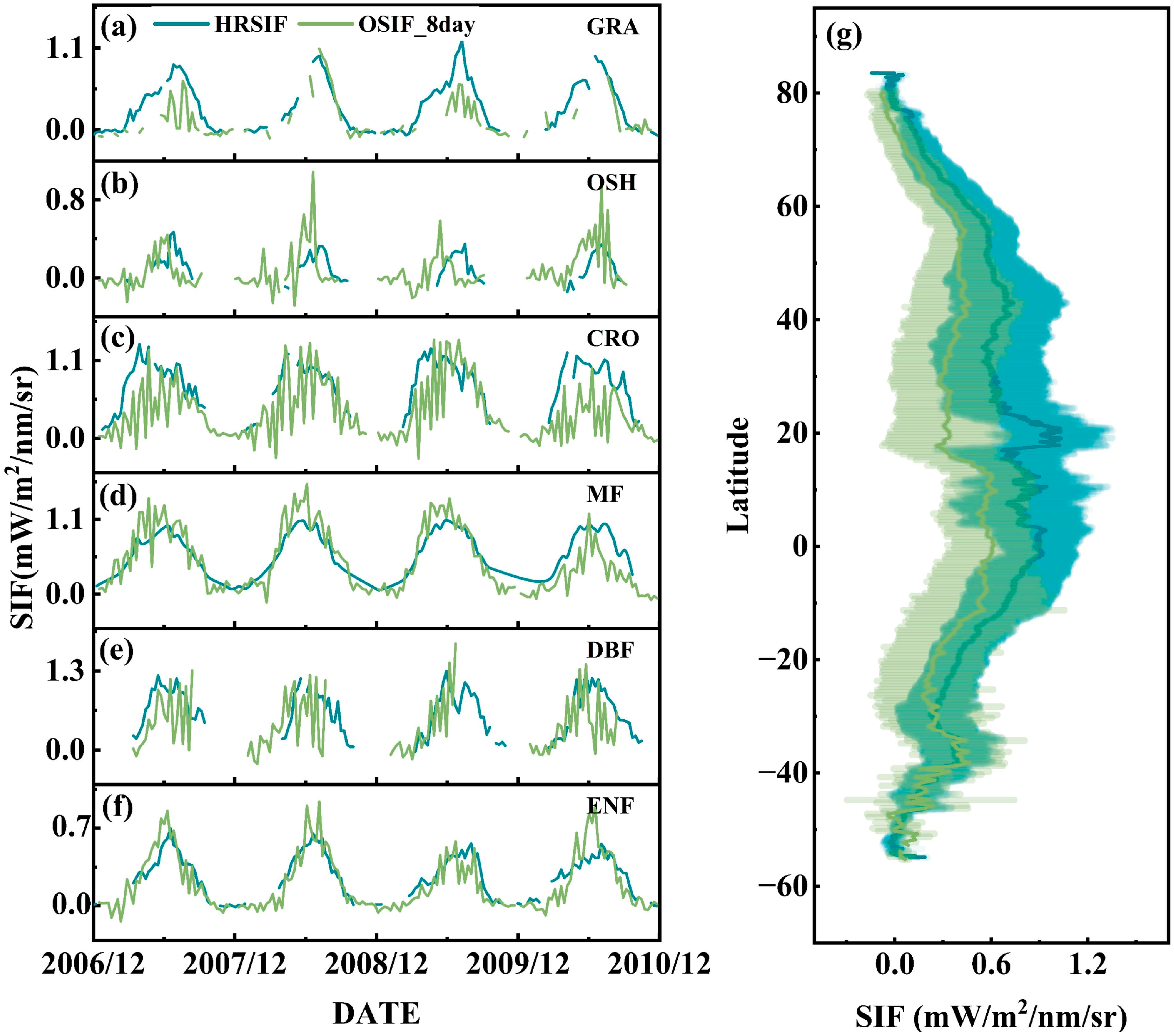
3.2.1. Comparison with Ground-Based Observations

Satellite SIF observation is a regional and large-scale remote sensing method. Therefore, to verify the accuracy of its data, it is necessary to conduct cross-validation using near-surface in situ observations. The downscaled SIF (hereinafter referred to as HRSIF) data can better meet the requirements for such comparisons. Considering the high-frequency daily observations at these sites, we calculated the average of all SIF measurements between 9:00 AM and 10:00 AM local time to represent the daily observation value, corresponding to the GOME-2 overpass time (approximately 9:30 AM). These daily values were then aggregated into 8-day averages to match the spatial and temporal resolution of the satellite data. The comparison between ground-based and satellite SIF data shows that their annual trends are highly consistent, with strong correlations between the two datasets, as shown in Figure 4. The US-NR1 and CA-OBS sites are both dominated by evergreen needleleaf forests (ENF), with highly consistent vegetation cover, leading to the strongest correlations. The Huailai and Jurong sites are cropland ecosystems, which are more affected by human activities, resulting in relatively lower correlations.
GOME-2 SIF data are retrieved at the 740 nm band, while ground-based SIF observation systems typically retrieve at the O2-A (760 nm) or O2-B (680 nm) bands. According to the shape of the SIF emission spectrum, there are two peaks at 685 nm and 740 nm, which differ in magnitude. Therefore, HRSIF and ground-based SIF observations exhibit consistent trends in Figure 4, but differ in magnitude. During the peak period from June to September, HRSIF values are significantly higher than those from ground-based observations. Yang et al. used the SCOPE model to derive a conversion factor of 0.58 between SIF at 740 nm (SIF740) and SIF at 760 nm (SIF760) [43]. In their study, GOME-2 SIF was multiplied by this factor and then compared with the observations from ground-based systems.

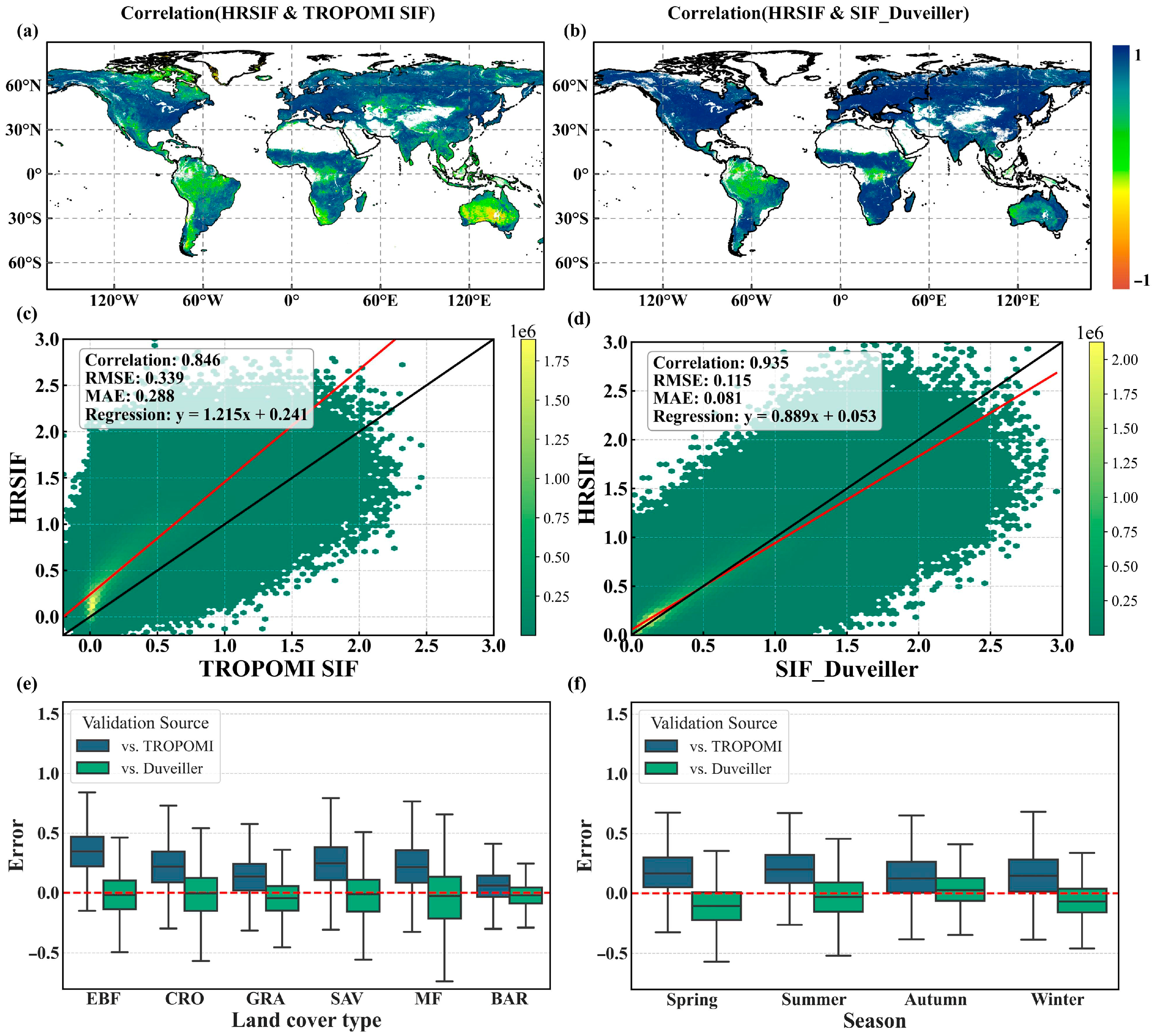
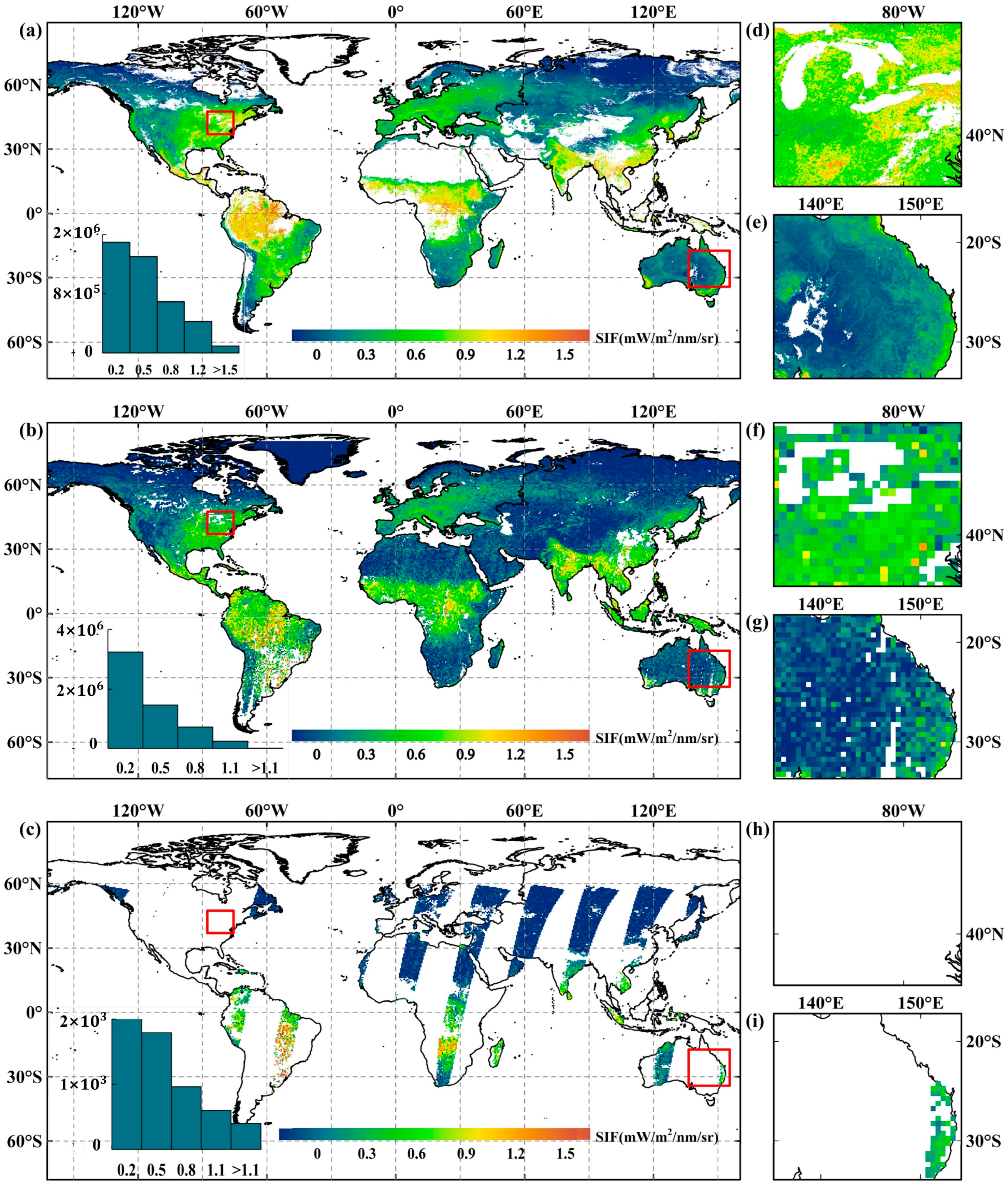
3.2.2. Comparison with Other Satellite Products

To evaluate the consistency of the HRSIF product generated in this study with other satellite products, we also compared the HRSIF product with the TROPOMI SIF and SIFDuveiller products. Spatial correlation analysis was conducted by calculating the time series correlation coefficients between each pair of products at each pixel location. The results show that the HRSIF product exhibits strong global consistency with both satellite products. The spatial distribution of the correlation coefficients between HRSIF and TROPOMI SIF is shown in Figure 5a, with a global correlation exceeding 0.80. The slope of the linear regression, shown in Figure 5c, is 1.2, which is close to one. Additionally, global statistical metrics between HRSIF and SIFDuveiller reveal a high correlation coefficient of 0.9352, with small RMSE and MAE values, as shown in Figure 5b,d. Both HRSIF and SIFDuveiller are based on GOME-2 SIF data and use different downscaling approaches. The high level of agreement between the final products indicates that the machine learning method adopted in this study can achieve comparable results to semi-empirical methods, effectively preserving the physiological information of the original SIF.
We also analyzed the errors between HRSIF and the two products under different land cover types and seasons, as shown in Figure 5e,f. Figure 5e randomly selected six different land cover types. The consistency between HRSIF and SIFDuveiller was generally higher than that between HRSIF and TROPOMI. However, GOME-2, with its coarse resolution, resulted in a relatively high deviation compared to TROPOMI during the pixel averaging process. As shown in Figure 5f, the differences between HRSIF and the two products were relatively consistent across different seasons, indicating that our HRSIF product exhibits good temporal stability.
It is worth noting that the spatial distribution of the correlation coefficients shows that the correlation between HRSIF and other products is lower in some tropical and arid regions. The primary reason is that persistent cloud cover in tropical rainforests leads to high levels of data noise, while in arid regions (such as deserts and barren lands), sparse vegetation, low photosynthetic activity, and strong soil background interference may result in greater errors [19,42]. Nevertheless, the strong correlation between HRSIF and the two satellite products in most parts of the world further confirms the validity and reliability of the method proposed in this study.

3.3. Characteristics of the Spatial and Temporal Distribution of HRSIF

Using the XGBoost-trained model, we generated a high-resolution SIF dataset (HRSIF) with a spatial resolution of 0.05° × 0.05° and an 8-day temporal resolution for the period from 2007 to 2020, presented in TIFF format. Taking the data from 14 September 2018 as an example, the grid-distributed pixel-level results are shown in Figure 6a. Figure 6b shows the 8-day average of the original GOME-2 SIF data (OSIF_8 day), and Figure 6c presents the original daily GOME-2 SIF data (OSIF). By comparison, HRSIF demonstrates significantly enhanced spatial detail and can reflect the internal heterogeneity of local ecosystems. For instance, Figure 6d reveals high SIF values over a small section of the U.S. Corn Belt, which are not discernible in Figure 6f,h. Similarly, in the detailed maps of Australia shown in Figure 6e,g,i, HRSIF clearly distinguishes differences in SIF values between agricultural areas and forests, as well as the high values in the eastern Great Dividing Range region—features that are typically averaged out or obscured in the original lower-resolution data.
To validate the correlation between the generated HRSIF and the original OSIF, six regions with different land cover types were randomly selected, as indicated by the red boxes in Figure 1. These regions span six continents, excluding Antarctica. Within each region, pixel-wise covariance and Pearson correlation coefficient matrices were calculated. As shown in Table 3, the results demonstrate a strong overall correlation between the downscaled HRSIF and the original SIF, with an average Pearson correlation of 0.76. In most regions, the correlation exceeds 0.6. However, lower correlation values were observed in Regions 2 and 6, which include arid and semi-arid areas.
This study also analyzes the distribution and variation in HRSIF from both spatial and temporal perspectives. Temporally, Figure 7a–f illustrate the time series trends of HRSIF and OSIF_8 day at different sites, representing six types of land cover: grassland, open shrublands, cropland, mixed forest, deciduous broadleaf forests, and evergreen needleleaf forests. The results show that HRSIF exhibits clear seasonal variation patterns that closely align with vegetation growth cycles. The SIF value continues to rise during the spring green-up period, reaches a clear peak during the summer growth season, and decreases during the autumn senescence period. This main seasonal rhythm proves that this dataset can effectively capture the basic dynamics of vegetation photosynthetic activity. Moreover, compared with the OSIF_8 day product, the time series of HRSIF shows a significantly smoother profile. This smoothness effectively filters out high-frequency noise while retaining the main seasonal and interannual trends, highlighting the robustness and clarity of the HRSIF dataset in long-term vegetation dynamic monitoring. Spatially, Figure 7g presents the latitudinal averages of HRSIF and OSIF_8 day. In the Northern Hemisphere, high SIF values are concentrated in mid-latitude regions, while in the Southern Hemisphere, they are more pronounced in low-latitude regions. Overall, the results in Figure 7 demonstrate strong consistency between HRSIF and OSIF_8 day across both spatial and temporal scales. This indicates that the downscaling algorithm preserves the original characteristics of SIF emissions, which is crucial for the reliability and application of the resulting data product.

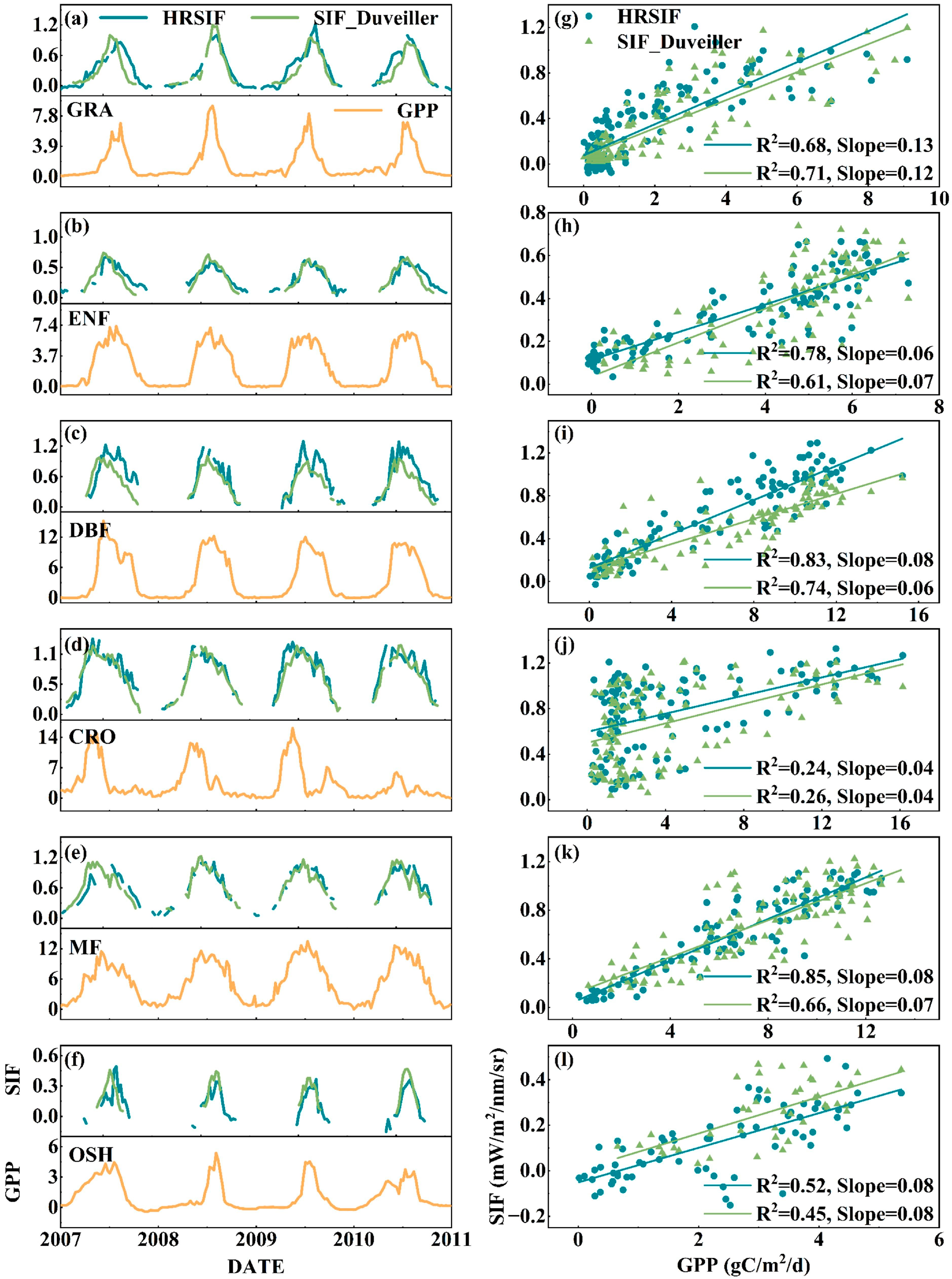
3.4. Correlation of HRSIF and GPP Under Different Land Use Types

As a novel remote sensing parameter, SIF exhibits a strong global linear relationship with GPP [44], making it an effective indicator of photosynthetic activity and terrestrial productivity. The high-resolution HRSIF product developed in this study can be further applied in climate-driven vegetation monitoring, carbon budgeting, and ecosystem stress assessment. Previous studies have statistically demonstrated the strong linear relationship between SIF and vegetation gross primary productivity (GPP) at both global and regional scales [45,46]. To validate the reliability of the downscaled HRSIF data generated in this study, we compared it with GPP derived from flux tower observations. In addition, to highlight the advantages of HRSIF in representing GPP, we also compared its relationship with that of SIFDuveiller and GPP. We used the FluxNet 2015 dataset [47], deriving GPP from observed NEE data collected by global eddy covariance flux towers, combined with ecosystem respiration. In this study, the average of daytime and nighttime-based calculations (GPP_DT_VUT_REF and GPP_NT_VUT_REF) was used as the final GPP value for each site, and aggregated into 8-day intervals to match the temporal resolution of HRSIF. The dataset also includes the land cover type of each site. By comparing with MODIS land cover data, we selected sites with homogeneous land cover types to ensure spatial consistency and reduce comparison errors. Ultimately, six flux tower sites with distinct vegetation types were selected, as shown in Table 4. The selected sites represent grassland (GRA), evergreen needleleaf forest (ENF), deciduous broadleaf forest (DBF), cropland (CRO), mixed forest (MF), and open shrubland (OSH).
Considering the coverage period of satellite SIF data and site-based GPP observations, the long-term trends of SIF and GPP were extracted from each selected site. At the 8-day temporal scale, HRSIF, SIFDuveiller, and GPP exhibit strong linear correlations and consistent annual trends at MF, DBF, ENF, and GRA sites (Figure 8). However, the correlation is relatively weaker at CRO and OSH sites, as shown in Figure 8j,l. This weaker correlation can be attributed to the need for long-term field management in croplands, where human activities such as irrigation and fertilization can significantly alter vegetation dynamics and physiological processes, introducing additional uncertainty in SIF-GPP estimation [48,49]. Most shrublands are located in arid regions, where vegetation is subject to strong drought stress and highly dynamic changes, which reconstructed SIF products may not capture effectively [50]. This can impair the correlation between SIF and GPP to some extent. Overall, HRSIF shows higher correlation with GPP than SIFDuveiller, indicating that the downscaled HRSIF product generated in this study provides a more accurate representation of GPP.

4. Discussion

4.1. The Necessity of Comparing Different Research Methods

Different model training methods have their strengths and limitations. Selecting the most appropriate algorithm based on specific research objectives is essential. Linear regression models exhibit limited predictive performance, as they struggle to effectively capture nonlinear features in the data. As shown in the training results in Section 3.1, the XGBoost and MLPRegressor models delivered the best performance. Since most parameters related to SIF can be derived from satellite observations, the types of input features used in the model are relatively consistent, and complex feature engineering is not required. Neural network models, due to their complex structure, demand higher computational resources and have lower training efficiency. However, they are advantageous for large and complex datasets where deep nonlinear relationships exist among features. Most current studies adopt neural network algorithms for regional downscaling [21], striking a balance between accuracy and efficiency. For global SIF downscaling tasks, tree-based models offer advantages such as faster training and simpler parameter tuning [19]. Overall, compared to other algorithms, XGBoost maintains excellent predictive performance while demonstrating superior training efficiency. Furthermore, while interpretability techniques like SHAP analysis are applicable to many models, including neural networks, their application to tree-based models like XGBoost is particularly computationally efficient and direct [51]. Therefore, by comprehensively considering its high prediction accuracy, computational efficiency, and practical, efficient interpretability, this study ultimately selects XGBoost as the optimal prediction model.
In addition, the HRSIF product generated in this study is based entirely on machine learning algorithms, whereas the SIFDuveiller product is derived from a semi-empirical approach that relies on predefined equations and parameter fitting, which may introduce uncertainties due to the assumptions inherent in those formulations. Compared to SIFDuveiller, the HRSIF product developed in this study offers several notable advantages. First, HRSIF employs a fully data-driven machine learning method that avoids dependence on prior assumptions from semi-empirical models, thereby reducing the risk of biases caused by model simplification. Second, by incorporating land cover classification data, the HRSIF approach can better adapt to the complex environmental characteristics of different regions. As shown in Section 3.1, the model performs well across various land cover types, which enhances its applicability to diverse ecosystems and allows for a more accurate representation of GPP, as demonstrated in Section 3.4. Moreover, this method provides flexibility to incorporate additional remote sensing variables into the training process, further improving its capacity to characterize the spatiotemporal variability of SIF.

4.2. Impact of the Choice of Explanatory Variables on the Model

In general, machine learning models are often criticized for their lack of interpretability compared to physical models. However, the XGBoost algorithm supports SHAP analysis, which enables a quantitative assessment of the impact of each feature variable on the model’s predictions. Previous studies have varied significantly in their selection of input features—some used a wide range of variable types, while others relied solely on surface reflectance [42]. The choice of input parameters typically depends on the target variable to be downscaled and the specific model. For instance, Li et al. [52] reported that land cover played only a minor role in their SIF prediction model. In this study, we conducted a SHAP-based interpretability analysis to quantitatively evaluate the contribution of each input feature to the model’s performance. As land cover type is a categorical variable, it cannot be ranked in terms of numerical value and is therefore displayed in gray in Figure 9. Nonetheless, its SHAP value still allows us to quantify its overall influence on the model’s output.
As shown in Figure 9, land cover data had a relatively smaller impact on the model’s output compared to variables such as NDVI and LST. However, during model training, we initially included MODIS land cover data as one of the input features and compared the model performance with and without this variable. We found that including land cover data improved the model’s performance across all evaluation metrics. This indicates that although land cover ranks lower in feature importance, its inclusion still has a positive effect on model training. Furthermore, as demonstrated in Section 3.4, our HRSIF product shows a stronger correlation with GPP compared to the SIFDuveiller product, which does not incorporate land cover information. This is because the land cover type can indirectly reflect vegetation structure and growth characteristics; removing this variable could reduce the model’s ability to distinguish between different ecosystems. This highlights a key advantage of machine learning models over empirical physical models: the flexibility to incorporate diverse types of input variables, including categorical data.

4.3. The Limitations of the Model and Future Improvements

While this study successfully demonstrates a method for SIF downscaling, we acknowledge several limitations that offer clear directions for future research. These limitations primarily concern the resolution of the input data, uncertainties from the downscaling methodology, and the source of data used for modeling and validation.
First, the accuracy of our final product was fundamentally constrained by the low spatiotemporal resolution of the GOME-2 SIF data. While coarse initial data limits achievable detail, long-term records like GOME-2 are invaluable for historical trend analysis. Previous studies have conducted downscaling processing by integrating SIF data from various sources [9]. One promising direction for future research is to combine the long-term observational records of GOME-2 with high-resolution data like TROPOMI. This approach would not only enhance the spatial resolution of the downscaled product but also generate a consistent, long-term, and verifiable SIF dataset, which is crucial for climate change and long-term ecosystem studies.
Secondly, machine learning methods often overlook local spatial attributes when analyzing spatial data. Although our explanatory variables provide geographic information, this can lead to the smoothing of fine-scale details. Future work should focus on optimizing the downscaling algorithm to better capture spatial heterogeneity. For instance, a hybrid model combining Geographically Weighted Regression (GWR) with machine learning could be highly effective [53]. GWR accounts for spatial non-stationarity, while machine learning can model complex nonlinear relationships, allowing the combined model to better address both spatial dependence and heterogeneity.
Finally, the model’s robustness and validation were limited by its reliance on a single auxiliary data source (MODIS) and the lack of ground-based validation [54]. To build a more robust model, future iterations could integrate multi-source auxiliary data, such as radar-based satellite products that are less sensitive to cloud cover [55], or dynamic variables like seasonal Leaf Area Index (LAI) to better differentiate land cover types. Crucially, validating the downscaled SIF products against direct, ground-based SIF measurements is the most critical next step. The expansion of global ground-based SIF observation networks will be invaluable not only for direct validation but also for data assimilation approaches that merge “ground truth” with satellite observations to produce a new generation of high-resolution, high-accuracy SIF products [56]. In addition, a key application of long-term SIF products is to monitor vegetation responses to extreme climate events such as drought. As a direct probe of photosynthesis, SIF is theoretically highly sensitive to drought stress. Recent studies have demonstrated this potential. For example, Chen et al. effectively monitored the impact of drought on agricultural systems using SIF time series data [57]. Han et al. also highlighted the value of integrating SIF data in rapid drought warning systems [58]. The high temporal resolution and long-term characteristics of the SIF products we have generated provide a solid foundation for capturing such stress signals. Although a comprehensive analysis of specific historical drought events is beyond the scope of this study, it will be a key direction for future research. Our subsequent work will focus on validating the performance of this product during well-documented drought periods to comprehensively assess its capabilities in monitoring extreme events.

5. Conclusions

In this study, the XGBoost algorithm was used to build a high-precision SIF prediction model by combining physiological and light-related variables, and to generate downscaled HRSIF products. The main conclusions of the study include (1) XGBoost shows superior performance in this task compared to several other algorithms. The model effectively improves the GOME-2 SIF coarse resolution data and performs well in different ecosystem types. (2) The reliability of the HRSIF product and the improvement in spatial details are highlighted by the dual validation of the ground-based sites and satellite products. (3) The HRSIF considering land use types showed a strong linear correlation with flux tower GPP observations, especially in mixed forest ecosystems (R2 = 0.85). In addition, we investigated the importance of individual input features to the model, highlighting the impact of land use type on model performance. These findings confirm the feasibility of applying machine learning to improve the spatial and temporal resolution of satellite SIF products and expand their utility in ecosystem productivity assessment.

Author Contributions

C.H.: Writing—original draft, Investigation, Methodology, Software, Data curation. P.X.: Conceptualization, Resources, Project administration, Funding acquisition, Validation, Writing—review and editing. Z.H.: Methodology, Funding acquisition, Writing—review and editing. A.L.: Investigation, Validation, Supervision, Writing—review and editing. H.F.: Investigation, Visualization. All authors have read and agreed to the published version of the manuscript.

Funding

This research was funded by the National Natural Science Foundation of China (grant numbers: 42030609 and 42105133), National Key Research and Development Program of China (grant numbers: 2022YFC3700300, 2022YFC3703502, and 2023YFC3705601), and Industrialization Project of Wanjiang Emerging Industry Technology Development Center (grant number: WJ21CYHXM03).

Data Availability Statement

The code for generating the HRSIF and relevant data are available at https://github.com/zzmxx/HRSIF.git (accessed on 3 June 2025).

Acknowledgments

We extend our gratitude to the scientists involved in the GOME-2 mission, as well as those responsible for the MODIS and CERES data products, for providing access to these valuable resources for the research community. Our appreciation also goes to the principal investigators and research staff at FLUXNET sites for sharing their flux data. This research utilized eddy covariance data collected and distributed by the FLUXNET community. We are grateful for the data provided by the researchers at the ChinaSpec sites, which mainly include Jurong and Huailai. We would also like to express our gratitude to Pierrat and colleagues for generously sharing the PhotoSpec site observation data and to Duveiller and colleagues for providing the downscaled GOME-2 data. Additionally, we are thankful to the anonymous reviewers for their insightful feedback on our manuscript.

Conflicts of Interest

The authors declare no conflicts of interest.

References

  1. Zhang, Z.; Cescatti, A.; Wang, Y.-P.; Gentine, P.; Xiao, J.; Guanter, L.; Huete, A.R.; Wu, J.; Chen, J.M.; Ju, W.; et al. Large Diurnal Compensatory Effects Mitigate the Response of Amazonian Forests to Atmospheric Warming and Drying. Sci. Adv. 2023, 9, eabq4974. [Google Scholar] [CrossRef]
  2. Li, W.; Pacheco-Labrador, J.; Migliavacca, M.; Miralles, D.; Hoek van Dijke, A.; Reichstein, M.; Forkel, M.; Zhang, W.; Frankenberg, C.; Panwar, A.; et al. Widespread and Complex Drought Effects on Vegetation Physiology Inferred from Space. Nat. Commun. 2023, 14, 4640. [Google Scholar] [CrossRef] [PubMed]
  3. Zarco-Tejada, P.J.; Poblete, T.; Camino, C.; Gonzalez-Dugo, V.; Calderon, R.; Hornero, A.; Hernandez-Clemente, R.; Román-Écija, M.; Velasco-Amo, M.P.; Landa, B.B.; et al. Divergent Abiotic Spectral Pathways Unravel Pathogen Stress Signals across Species. Nat. Commun. 2021, 12, 6088. [Google Scholar] [CrossRef] [PubMed]
  4. Joiner, J.; Yoshida, Y.; Vasilkov, A.P.; Yoshida, Y.; Corp, L.A.; Middleton, E.M. First Observations of Global and Seasonal Terrestrial Chlorophyll Fluorescence from Space. Biogeosciences 2011, 8, 637–651. [Google Scholar] [CrossRef]
  5. Sun, Y.; Frankenberg, C.; Wood, J.D.; Schimel, D.S.; Jung, M.; Guanter, L.; Drewry, D.T.; Verma, M.; Porcar-Castell, A.; Griffis, T.J.; et al. OCO-2 Advances Photosynthesis Observation from Space via Solar-Induced Chlorophyll Fluorescence. Science 2017, 358, eaam5747. [Google Scholar] [CrossRef]
  6. Köhler, P.; Frankenberg, C.; Magney, T.S.; Guanter, L.; Joiner, J.; Landgraf, J. Global Retrievals of Solar-Induced Chlorophyll Fluorescence With TROPOMI: First Results and Intersensor Comparison to OCO-2. Geophys. Res. Lett. 2018, 45, 10456–10463. [Google Scholar] [CrossRef]
  7. Zhang, Z.; Guanter, L.; Porcar-Castell, A.; Rossini, M.; Pacheco-Labrador, J.; Zhang, Y. Global Modeling Diurnal Gross Primary Production from OCO-3 Solar-Induced Chlorophyll Fluorescence. Remote Sens. Environ. 2023, 285, 113383. [Google Scholar] [CrossRef]
  8. Buareal, K.; Kato, T.; Morozumi, T.; Ono, K.; Nakashima, N. Red Solar-Induced Chlorophyll Fluorescence as a Robust Proxy for Ecosystem-Level Photosynthesis in a Rice Field. Agric. For. Meteorol. 2023, 336, 109473. [Google Scholar] [CrossRef]
  9. Wen, J.; Köhler, P.; Duveiller, G.; Parazoo, N.C.; Magney, T.S.; Hooker, G.; Yu, L.; Chang, C.Y.; Sun, Y. A Framework for Harmonizing Multiple Satellite Instruments to Generate a Long-Term Global High Spatial-Resolution Solar-Induced Chlorophyll Fluorescence (SIF). Remote Sens. Environ. 2020, 239, 111644. [Google Scholar] [CrossRef]
  10. Ma, Y.; Liu, L.; Liu, X.; Chen, J. An Improved Downscaled Sun-Induced Chlorophyll Fluorescence (DSIF) Product of GOME-2 Dataset. Eur. J. Remote Sens. 2022, 55, 168–180. [Google Scholar] [CrossRef]
  11. Chen, S.; Liu, L.; Sui, L.; Liu, X.; Ma, Y. An Improved Spatially Downscaled Solar-Induced Chlorophyll Fluorescence Dataset from the TROPOMI Product. Sci. Data 2025, 12, 135. [Google Scholar] [CrossRef]
  12. Chen, X.; Huang, Y.; Nie, C.; Zhang, S.; Wang, G.; Chen, S.; Chen, Z. A Long-Term Reconstructed TROPOMI Solar-Induced Fluorescence Dataset Using Machine Learning Algorithms. Sci. Data 2022, 9, 427. [Google Scholar] [CrossRef]
  13. Li, X.; Xiao, J. Mapping Photosynthesis Solely from Solar-Induced Chlorophyll Fluorescence: A Global, Fine-Resolution Dataset of Gross Primary Production Derived from OCO-2. Remote Sens. 2019, 11, 2563. [Google Scholar] [CrossRef]
  14. Duveiller, G.; Cescatti, A. Spatially Downscaling Sun-Induced Chlorophyll Fluorescence Leads to an Improved Temporal Correlation with Gross Primary Productivity. Remote Sens. Environ. 2016, 182, 72–89. [Google Scholar] [CrossRef]
  15. Yu, L.; Wen, J.; Chang, C.Y.; Frankenberg, C.; Sun, Y. High-Resolution Global Contiguous SIF of OCO-2. Geophys. Res. Lett. 2019, 46, 1449–1458. [Google Scholar] [CrossRef]
  16. Running, S.W.; Nemani, R.R.; Heinsch, F.A.; Zhao, M.; Reeves, M.; Hashimoto, H. A Continuous Satellite-Derived Measure of Global Terrestrial Primary Production. BioScience 2004, 54, 547–560. [Google Scholar] [CrossRef]
  17. Impollonia, G.; Croci, M.; Amaducci, S. Upscaling and Downscaling Approaches for Early Season Rice Yield Prediction Using Sentinel-2 and Machine Learning for Precision Nitrogen Fertilisation. Comput. Electron. Agric. 2024, 227, 109603. [Google Scholar] [CrossRef]
  18. Sorkhabi, O.M.; Awange, J. Long Short-Term Memory Exploitation of Satellite Gravimetry to Infer Floods. Int. J. Appl. Earth Obs. Geoinf. 2025, 139, 104562. [Google Scholar] [CrossRef]
  19. He, S.; Yuan, Y.; Dong, H.; Chen, X.; Zhang, C. A Geographically Random Machine Learning Model for GOME-2 Global Seamless Sun-Induced Chlorophyll Fluorescence Downscaling Products With High Spatiotemporal Resolution. IEEE Trans. Geosci. Remote Sens. 2025, 63, 1–15. [Google Scholar] [CrossRef]
  20. Grinsztajn, L.; Oyallon, E.; Varoquaux, G. Why Do Tree-Based Models Still Outperform Deep Learning on Tabular Data? arXiv 2022, arXiv:2207.08815. [Google Scholar]
  21. Gensheimer, J.; Turner, A.J.; Köhler, P.; Frankenberg, C.; Chen, J. A Convolutional Neural Network for Spatial Downscaling of Satellite-Based Solar-Induced Chlorophyll Fluorescence (SIFnet). Biogeosciences 2022, 19, 1777–1793. [Google Scholar] [CrossRef]
  22. Saha, S.; Roy, J.; Hembram, T.K.; Pradhan, B.; Dikshit, A.; Abdul Maulud, K.N.; Alamri, A.M. Comparison between Deep Learning and Tree-Based Machine Learning Approaches for Landslide Susceptibility Mapping. Water 2021, 13, 2664. [Google Scholar] [CrossRef]
  23. Zhang, Y.; Zhang, Q.; Liu, L.; Zhang, Y.; Wang, S.; Ju, W.; Zhou, G.; Zhou, L.; Tang, J.; Zhu, X.; et al. ChinaSpec: A Network for Long-Term Ground-Based Measurements of Solar-Induced Fluorescence in China. J. Geophys. Res. Biogeosci. 2021, 126, e2020JG006042. [Google Scholar] [CrossRef]
  24. Schaaf, C.; Wang, Z. MODIS/Terra+Aqua BRDF/Albedo Nadir BRDF-Adjusted Ref Daily L3 Global 0.05Deg CMG V061; NASA Land Processes Distributed Active Archive Center: Sioux Falls, SD, USA, 2021. [Google Scholar]
  25. Wan, Z.; Hook, S.; Hulley, G. MODIS/Terra Land Surface Temperature/Emissivity Daily L3 Global 0.05Deg CMG V061; NASA Land Processes Distributed Active Archive Center: Sioux Falls, SD, USA, 2021. [Google Scholar]
  26. Friedl, M.; Sulla-Menashe, D. MODIS/Terra+Aqua Land Cover Type Yearly L3 Global 0.05Deg CMG V061; NASA Land Processes Distributed Active Archive Center: Sioux Falls, SD, USA, 2022. [Google Scholar]
  27. Wielicki, B.A.; Barkstrom, B.R.; Harrison, E.F.; Lee, R.B.; Smith, G.L.; Cooper, J.E. Clouds and the Earth’s Radiant Energy System (CERES): An Earth Observing System Experiment. Bull. Am. Meteorol. Soc. 1996, 77, 853–868. [Google Scholar] [CrossRef]
  28. Joiner, J.; Guanter, L.; Lindstrot, R.; Voigt, M.; Vasilkov, A.P.; Middleton, E.M.; Huemmrich, K.F.; Yoshida, Y.; Frankenberg, C. Global Monitoring of Terrestrial Chlorophyll Fluorescence from Moderate-Spectral-Resolution near-Infrared Satellite Measurements: Methodology, Simulations, and Application to GOME-2. Atmos. Meas. Tech. 2013, 6, 2803–2823. [Google Scholar] [CrossRef]
  29. Köhler, P.; Guanter, L.; Joiner, J. A Linear Method for the Retrieval of Sun-Induced Chlorophyll Fluorescence from GOME-2 and SCIAMACHY Data. Atmos. Meas. Tech. 2015, 8, 2589–2608. [Google Scholar] [CrossRef]
  30. Grossmann, K.; Frankenberg, C.; Magney, T.S.; Hurlock, S.C.; Seibt, U.; Stutz, J. PhotoSpec: A New Instrument to Measure Spatially Distributed Red and Far-Red Solar-Induced Chlorophyll Fluorescence. Remote Sens. Environ. 2018, 216, 311–327. [Google Scholar] [CrossRef]
  31. Du, S.; Liu, L.; Liu, X.; Guo, J.; Hu, J.; Wang, S.; Zhang, Y. SIFSpec: Measuring Solar-Induced Chlorophyll Fluorescence Observations for Remote Sensing of Photosynthesis. Sensors 2019, 19, 3009. [Google Scholar] [CrossRef] [PubMed]
  32. Magney, T.; Frankenberg, C.; Stutz, J.; Grossmann, K. PhotoSpec Solar-Induced Fluorescence and Meteorological Data: Corn, Iowa. 2017. Available online: https://data.caltech.edu/records/em9wn-ntq87 (accessed on 27 July 2025).
  33. Pierrat, Z.; Stutz, J. Tower-Based Solar-Induced Fluorescence and Vegetation Index Data for Southern Old Black Spruce Forest. Available online: https://zenodo.org/records/7596931 (accessed on 27 July 2025).
  34. Zhang, Q.; Zhang, X.; Li, Z.; Wu, Y.; Zhang, Y. Comparison of Bi-Hemispherical and Hemispherical-Conical Configurations for In Situ Measurements of Solar-Induced Chlorophyll Fluorescence. Remote Sens. 2019, 11, 2642. [Google Scholar] [CrossRef]
  35. Liu, X.; Liu, L.; Bacour, C.; Guanter, L.; Chen, J.; Ma, Y.; Chen, R.; Du, S. A Simple Approach to Enhance the TROPOMI Solar-Induced Chlorophyll Fluorescence Product by Combining with Canopy Reflected Radiation at near-Infrared Band. Remote Sens. Environ. 2023, 284, 113341. [Google Scholar] [CrossRef]
  36. Duveiller, G.; Filipponi, F.; Walther, S.; Köhler, P.; Frankenberg, C.; Guanter, L.; Cescatti, A. A Spatially Downscaled Sun-Induced Fluorescence Global Product for Enhanced Monitoring of Vegetation Productivity. Earth Syst. Sci. Data 2020, 12, 1101–1116. [Google Scholar] [CrossRef]
  37. Chen, T.; Guestrin, C. XGBoost: A Scalable Tree Boosting System. In Proceedings of the 22nd ACM SIGKDD International Conference on Knowledge Discovery and Data Mining, San Francisco, CA, USA, 13–17 August 2016; Association for Computing Machinery: New York, NY, USA, 2016; pp. 785–794. [Google Scholar]
  38. Liu, X.; Guanter, L.; Liu, L.; Damm, A.; Malenovsky, Z.; Rascher, U.; Peng, D.; Du, S.; Gastellu-Etchegorry, J.-P. Downscaling of Solar-Induced Chlorophyll Fluorescence from Canopy Level to Photosystem Level Using a Random Forest Model. Remote Sens. Environ. 2019, 231, 110772. [Google Scholar] [CrossRef]
  39. Hesterman, J.Y.; Caucci, L.; Kupinski, M.A.; Barrett, H.H.; Furenlid, L.R. Maximum-Likelihood Estimation With a Contracting-Grid Search Algorithm. IEEE Trans. Nucl. Sci. 2010, 57, 1077–1084. [Google Scholar] [CrossRef]
  40. Li, X.; Xiao, J.; He, B.; Altaf Arain, M.; Beringer, J.; Desai, A.R.; Emmel, C.; Hollinger, D.Y.; Krasnova, A.; Mammarella, I.; et al. Solar-Induced Chlorophyll Fluorescence Is Strongly Correlated with Terrestrial Photosynthesis for a Wide Variety of Biomes: First Global Analysis Based on OCO-2 and Flux Tower Observations. Glob. Change Biol. 2018, 24, 3990–4008. [Google Scholar] [CrossRef]
  41. Huete, A.R.; Didan, K.; Shimabukuro, Y.E.; Ratana, P.; Saleska, S.R.; Hutyra, L.R.; Yang, W.; Nemani, R.R.; Myneni, R. Amazon Rainforests Green-up with Sunlight in Dry Season. Geophys. Res. Lett. 2006, 33, L06405. [Google Scholar] [CrossRef]
  42. Gentine, P.; Alemohammad, S.H. Reconstructed Solar-Induced Fluorescence: A Machine Learning Vegetation Product Based on MODIS Surface Reflectance to Reproduce GOME-2 Solar-Induced Fluorescence. Geophys. Res. Lett. 2018, 45, 3136–3146. [Google Scholar] [CrossRef] [PubMed]
  43. Damm, A.; Elbers, J.; Erler, A.; Gioli, B.; Hamdi, K.; Hutjes, R.; Kosvancova, M.; Meroni, M.; Miglietta, F.; Moersch, A.; et al. Remote Sensing of Sun-Induced Fluorescence to Improve Modeling of Diurnal Courses of Gross Primary Production (GPP). Glob. Change Biol. 2010, 16, 171–186. [Google Scholar] [CrossRef]
  44. Zeng, Y.; Hao, D.; Huete, A.; Dechant, B.; Berry, J.; Chen, J.M.; Joiner, J.; Frankenberg, C.; Bond-Lamberty, B.; Ryu, Y.; et al. Optical Vegetation Indices for Monitoring Terrestrial Ecosystems Globally. Nat. Rev. Earth Environ. 2022, 3, 477–493. [Google Scholar] [CrossRef]
  45. Yu, J.; Li, X.; Du, H.; Mao, F.; Xu, Y.; Huang, Z.; Zhao, Y.; Lv, L.; Song, M.; Huang, L.; et al. Solar-Induced Fluorescence-Based Phenology of Subtropical Forests in China and Its Response to Climate Factors. Agric. For. Meteorol. 2024, 356, 110182. [Google Scholar] [CrossRef]
  46. Zhu, W.; Xie, Z.; Zhao, C.; Zheng, Z.; Qiao, K.; Peng, D.; Fu, Y.H. Remote Sensing of Terrestrial Gross Primary Productivity: A Review of Advances in Theoretical Foundation, Key Parameters and Methods. GISci. Remote Sens. 2024, 61, 2318846. [Google Scholar] [CrossRef]
  47. Pastorello, G.; Trotta, C.; Canfora, E.; Chu, H.; Christianson, D.; Cheah, Y.-W.; Poindexter, C.; Chen, J.; Elbashandy, A.; Humphrey, M.; et al. The FLUXNET2015 Dataset and the ONEFlux Processing Pipeline for Eddy Covariance Data. Sci. Data 2020, 7, 225. [Google Scholar] [CrossRef]
  48. Martini, D.; Pacheco-Labrador, J.; Perez-Priego, O.; van der Tol, C.; El-Madany, T.S.; Julitta, T.; Rossini, M.; Reichstein, M.; Christiansen, R.; Rascher, U.; et al. Nitrogen and Phosphorus Effect on Sun-Induced Fluorescence and Gross Primary Productivity in Mediterranean Grassland. Remote Sens. 2019, 11, 2562. [Google Scholar] [CrossRef]
  49. Xu, E.; Zhou, L.; Ding, J.; Zhao, N.; Zeng, L.; Zhang, G.; Chi, Y. Physiological Dynamics Dominate the Relationship between Solar-Induced Chlorophyll Fluorescence and Gross Primary Productivity along the Nitrogen Gradient in Cropland. Sci. Total Environ. 2024, 929, 172725. [Google Scholar] [CrossRef]
  50. Wen, J.; Tagliabue, G.; Rossini, M.; Fava, F.P.; Panigada, C.; Merbold, L.; Leitner, S.; Sun, Y. Detection of Fast-Changing Intra-Seasonal Vegetation Dynamics of Drylands Using Solar-Induced Chlorophyll Fluorescence (SIF). Biogeosciences 2025, 22, 2049–2067. [Google Scholar] [CrossRef]
  51. Lundberg, S.M.; Lee, S.I. A Unified Approach to Interpreting Model Predictions. In Proceedings of the Neural Information Processing Systems, Long Beach, CA, USA, 4–9 December 2017. [Google Scholar]
  52. Li, X.; Xiao, J.; He, B. Chlorophyll Fluorescence Observed by OCO-2 Is Strongly Related to Gross Primary Productivity Estimated from Flux Towers in Temperate Forests. Remote Sens. Environ. 2018, 204, 659–671. [Google Scholar] [CrossRef]
  53. Grekousis, G. Geographical-XGBoost: A New Ensemble Model for Spatially Local Regression Based on Gradient-Boosted Trees. J. Geogr. Syst. 2025, 27, 169–195. [Google Scholar] [CrossRef]
  54. Lu, J.; Li, J.; Fu, H.; Zou, W.; Kang, J.; Yu, H.; Lin, X. Estimation of Rice Yield Using Multi-Source Remote Sensing Data Combined with Crop Growth Model and Deep Learning Algorithm. Agric. For. Meteorol. 2025, 370, 110600. [Google Scholar] [CrossRef]
  55. Ebel, P.; Meraner, A.; Schmitt, M.; Zhu, X.X. Multisensor Data Fusion for Cloud Removal in Global and All-Season Sentinel-2 Imagery. IEEE Trans. Geosci. Remote Sens. 2021, 59, 5866–5878. [Google Scholar] [CrossRef]
  56. Fang, L.; Jin, J.; Segers, A.; Li, K.; Xia, J.; Han, W.; Li, B.; Lin, H.X.; Zhu, L.; Liu, S.; et al. Observational Operator for Fair Model Evaluation with Ground NO2 Measurements. Geosci. Model. Dev. 2024, 17, 8267–8282. [Google Scholar] [CrossRef]
  57. Chen, Y.; Wang, Y.; Wu, C.; Jardim, A.M.d.R.F.; Fang, M.; Yao, L.; Liu, G.; Xu, Q.; Chen, L.; Tang, X. Drought-Induced Stress on Rainfed and Irrigated Agriculture: Insights from Multi-Source Satellite-Derived Ecological Indicators. Agric. Water Manag. 2025, 307, 109249. [Google Scholar] [CrossRef]
  58. Han, L.; Chen, Y.; Wu, C.; Yao, L.; Wang, Y.; Su, C.; Li, X.; da Rosa Ferraz Jardim, A.M.; Freire da Silva, T.G.; Tang, X. Divergent Drought-Induced Suppression on Vegetation and Associated Feedbacks: Satellite-Based Observations in 2022 across the Yangtze River Basin, China. J. Hydrol. 2025, 661, 133673. [Google Scholar] [CrossRef]
Figure 1. Global land use/land cover (LULC) map and the six regions where HRSIF was compared to the original 8-day synthetic GOME-2 SIF (red boxes). The LULC types and their abbreviations represented by the numbers in the IGBP classification of the MCD12C1 product: 0 water bodies (WAT), 1 evergreen needleleaf forests (ENF), 2 evergreen broadleaf forests (EBF), 3 deciduous needleleaf forests (DNF), 4 deciduous broadleaf forests (EBF), 5 mixed forests (MF), 6 closed shrublands (CSH), 7 open shrublands (OSH), 8 woody savannas (WSA), 9 savannas (SAV), 10 grasslands (GRA), 11 wetlands (WET), 12 croplands (CRO), 13 urban and built-up (URB), 14 cropland/nature vegetation mosaic (CVM), 15 snow and ice (SNO), 16 barren sparse vegetation (BSV).
Remotesensing 17 02642 g001
Figure 2. Research flowchart.
Remotesensing 17 02642 g002
Figure 3. Model training results. (ad) represents the training results of four different models: MLR, RF, MLPRegressor, and XGBoost; (eg) shows the parameter tuning process of XGBoost, and (hj) shows the performance evaluation of the XGBoost model under different land use types.
Remotesensing 17 02642 g003
Figure 4. Trends and correlations between HRSIF and ground-based observations at the 8-day scale. The unit of SIF is mW/m2/nm/sr. (a,b) The US-NR1 site; (c,d) The CA-OBS site; (e,f) The Huailai site; (g,h) The Jurong site.
Remotesensing 17 02642 g004
Figure 5. Global distribution map of Pearson correlation coefficients and density scatter plots of correlation. (a) Correlation between HRSIF and TROPOMI eSIF. (b) Correlation between HRSIF and SIFDuveiller. (c) The verification scatter plot of the correlation between HRSIF and TROPOMI eSIF for all pixel points worldwide over a one-year period. (d) The verification scatter plot of the correlation between HRSIF and SIFDuveiller for all pixel points worldwide over a one-year period. (e) The errors of HRSIF in different ecosystems compared with TROPOMI eSIF and SIFDuveiller. (f) The errors of HRSIF compared with TROPOMI eSIF and SIFDuveiller in different seasons.
Remotesensing 17 02642 g005
Figure 6. Spatial distribution and detailed views of HRSIF, OSIF_8 day, and OSIF. (a,d,e) show the downscaled HRSIF data; (b,f,g) represent the 8-day averaged original GOME-2 SIF data (OSIF_8 day); (c,h,i) display the original daily GOME-2 SIF data (OSIF).
Remotesensing 17 02642 g006
Figure 7. Spatiotemporal distribution of HRSIF and OSIF_8 day. (af) Temporal variations in HRSIF and OSIF_8 day at different land cover type sites from 2007 to 2010; (g) Latitudinal distribution of HRSIF and OSIF_8 day.
Remotesensing 17 02642 g007
Figure 8. Temporal trends and correlations of HRSIF, SIFDuveiller, and GPP at different sites. (af) Multi-year temporal trends of HRSIF, SIFDuveiller, and GPP for six common vegetation types: GRA, ENF, DBF, CRO, MF, and OSH. (gl) Linear regression plots of SIF versus GPP at the corresponding sites.
Remotesensing 17 02642 g008
Figure 9. Analysis of SHAP values of model parameters and the effect of land use parameters on training effectiveness. (a) The SHAP values of each input parameter ranked by their importance. (b) RMSE changes for model training with land use parameters included. (c) Model RMSE variation without land use parameters.
Remotesensing 17 02642 g009
Table 1. Model input data.
DataResolutionDescriptionSource
MCD43C40.05° × 0.05°NBAR: Nadir BRDF-Adjusted Reflectance https://lpdaac.usgs.gov/products/mcd43c4v061/ (accessed on 5 June 2025)
MOD11C10.05° × 0.05°LST: Land Surface Temperaturehttps://lpdaac.usgs.gov/products/mod11c1v061/ (accessed on 5 June 2025)
CERES_SYN1deg1° × 1°PAR: Photosynthetically Active Radiationhttps://ceres.larc.nasa.gov/data/# (accessed on 5 June 2025)
MCD12C10.05° × 0.05°IGBP classification: Land Use/Land Cover typehttps://lpdaac.usgs.gov/products/mcd12c1v061/ (accessed on 5 June 2025)
GOME-2 SIF0.5° × 0.5°SIF: Sun-induced chlorophyll Fluorescenceftp://ftp.gfz-potsdam.de/home/mefe/GlobFluo/ (accessed on 5 June 2025)
Table 2. List of the optimal hyperparameters of the XGBoost model.
ParametersValue
n_estimators3500
min_child_weight3
max_depth6
learning_rate0.05
tree_methodgpu_hist
Table 3. The list of Pearson correlation coefficients between HRSIF and OSIF in the selected regions.
RegionPearson
Region 10.67
Region 20.35
Region 30.65
Region 40.72
Region 50.78
Region 60.51
All regions0.76
Table 4. List of flux observation stations.
SitesIGBP TypeLatitudeLongitude
CN-CNGGRA44.59123.51
CA-OBSENF53.99−105.12
US-UMBDBF45.56−84.71
CH-OE2CRO47.297.73
BE-VIEMF50.305.99
RU-COKOSH70.83147.49
Disclaimer/Publisher’s Note: The statements, opinions and data contained in all publications are solely those of the individual author(s) and contributor(s) and not of MDPI and/or the editor(s). MDPI and/or the editor(s) disclaim responsibility for any injury to people or property resulting from any ideas, methods, instructions or products referred to in the content.

