Analysis of the Dynamic Process of Tornado Formation on 28 July 2024

Abstract

An EF1 tornado struck Nansha District, Guangzhou, Guangdong, on 28 July 2024. To explore the dynamic and thermodynamic changes during the tornado’s life cycle, high-resolution spatiotemporal data from Foshan’s X-band phased-array radar and the direct wind field synthesis algorithm were used to reconstruct the 3D wind field. The dynamics and 3D structure of the tornado were analysed, with a new parameter, vorticity volume (VV), introduced to study its variation. The observation results indicate that the tornado moved from southwest to northeast. During the tornado’s early stage (00:10–00:20 UTC), arc-shaped and annular echoes emerged and positive vorticity increased (peaking at 0.042 s⁻¹). Based on the tornado’s movement direction, the right side of the vortex centre was divergent, while the left side was convergent, whereas the vorticity area and volume continued to grow centrally. During the mature stage (00:23–00:25 UTC), the echo intensity weakened and, at 00:24, the vorticity reached its peak and touched the ground, with the vorticity area and volume also reaching their peaks at the same time. During the dissipation stage (00:25–00:30 UTC), the vorticity and echo features faded and the vorticity area and volume also declined rapidly. The analysis showed that the vorticity volume effectively reflects the tornado’s life cycle, enhancing the understanding of the dynamic and thermodynamic processes during the tornado’s development.

1. Introduction

As a small-scale weather phenomenon with strong destructive power in nature, a tornado has the characteristics of small spatial scale, short life cycle and strong suddenness. Accurately detecting and receiving early warnings for tornados has been an international problem in the field of meteorology for some time [1]. In-depth investigation into the formation mechanism of tornadoes and the timely release of short-range warning information are crucial for enhancing disaster prevention and mitigation capabilities [2].

Brian [3] showed that tornadoes are often accompanied by mesoscale convective systems (MCSs), which require a combination of low-altitude convergence, vertical wind shear (>20 m/s) and convective effective potential energy (CAPE > 1500 J/kg). In the 1980s, a new generation of Doppler-effect weather radar, the WSR-88D, was developed in the USA [4,5], whose S-band radar significantly improved storm observation capabilities. In addition, after 2007, the WSR-88D was upgraded with dual-polarisation [6], which improved the accuracy of its precipitation estimation and tornado identification through the application of dual-polarisation products [7,8]. At the end of the 20th Century, scientists proposed a conceptual model of a tornado structure based on radar observations [9], identifying key structures, such as mesocyclones and the tornado vortex signature (TVS). In the 21st Century, high-precision radar has revealed the detailed evolution of tornadoes, such as the interaction between the rear-facing downdraft (RFD) and the tornado vortex [10].

According to statistics, the number of tornadoes occurring in China each year is less than one-tenth of that in the United States [11]. At the end of the 20th Century, relatively few studies on tornadoes were conducted in China due to limited monitoring levels and capability [12]. At the beginning of the 21st Century, with the application of Doppler radar and satellites and numerical models (e.g., WRF and ARPS), the analyses of tornadoes in terms of their structure, environmental conditions and dynamical mechanisms gradually deepened [13]. Using Doppler weather radar data, Liu Juan et al. [14] analysed the tornado weather occurring in Tianchang, Anhui Province and Gaoyou, Jiangsu Province, and they explored the typical characteristics of products such as mesocyclone and tornado vortex signature (TVS). The joint appearance of TVS with strong medium cyclones or medium-intensity medium cyclones can be used as a criterion for the intensity of tornadoes. Song Zizhong et al. [15], while analysing a severe tornado event that occurred in Lingbi County on the afternoon of 30 July 2005, revealed the vortex characteristics associated with a strong tornado by comparing and analysing radar data from Fuyang and Xuzhou. In a new generation weather radar business application paper collection, Yu Xiaoding [16] confirmed the conclusion proposed by Brooks et al. [17] that strong low-level vertical wind shear and low lifting condensation height are favourable for the generation of strong tornadoes. Hu Yuling et al. [18] studied the tornado weather process that occurred in Anhui on the afternoon of 3 July 2007, and they found that low-level vertical wind shear (0–1 km) is the key factor for tornado formation. Wu Fangfang et al. [19] analysed the Doppler radar echo characteristics of 72 supercell storms in northern Jiangsu and concluded that, in tornado identification and warning, echo intensity is not entirely related to tornado intensity. Tornado warning should mainly be based on mesocyclones and strong rotational echoes (TVS). The lower the bottom and the smaller the diameter of a mesocyclone, the more likely it is to produce a tornado. Zhou Haiguang et al. [20] used dual-Doppler radar-derived three-dimensional wind fields to analyse the EF4 tornado in Funing, Jiangsu, China on 23 June 2016, and they also studied the three-dimensional structure and evolution characteristics of the supercell storm of this tornado. Gu Yu et al. [21] analysed the radar echo characteristics, supercell structure and evolution characteristics of the super-strong tornado in Funing, Jiangsu, using Doppler radar and satellite data, and they found that a tornado occurs at the time of the maximum increase in the thickness of the 3D circulation and the maximum shear jump. Akira’s simulation study showed that the horizontal vorticity generated by environmental wind shear is tilted to the vertical direction in the lower layers of the storm (<1 km) and it is amplified by the stretching of the updraft, forming strong rotation. For example, in the 2003 Oklahoma City supercell simulation, the horizontal vorticity generated by surface friction was tilted into vertical vorticity, becoming the primary source of the tornado vortex [22]. Through fully physical supercell simulations and highly idealised simulations, Jannick Fischer et al. revealed two main dynamical mechanisms in the formation of tornadoes: the subsidence mechanism and the internal upwards mechanism. Their study found that, during the early stages of tornado formation, the extremes of vertical vorticity are primarily generated through the sinking airflow mechanism, while the fully developed vortex dynamics are primarily dominated by the internal ascending mechanism. There is a clear transition between these two mechanisms, which is closely related to the process of the axisymmetricisation of the pre-tornado vortex patch and its strengthening through vertical stretching [23].

With the continuous increase in the timeliness and precision requirements for the study of severe convective weather, Doppler weather radar can no longer adequately meet the needs of identifying and warning of tornadoes and other small-scale weather systems. Therefore, phased-array radar with high spatiotemporal resolution is important for identifying and receiving warnings of small-scale severe convective weather such as tornadoes. In Kansas, US, the mobile phased-array radar MWR-05XP first observed a tornado, capturing the wind speed change (from 20 m/s to 36 m/s) and anticyclonic vortex characteristics during the tornado’s life cycle [24]. In the El Reno EF5 tornado event, compared with the WSR-88D radar, S-band PAR data show that the rapid scanning of PAR can identify the strengthening of mesocyclones and the sudden change of tornado paths earlier, gaining key time for warnings [25]. Using phased-array weather radar composed of three or more phased-array transceiver front ends can yield high-resolution intensity and 3D wind fields, offering technical support for analysing severe convective weather [26,27,28,29]. In the Pearl River Estuary waterspout event, X-band dual-polarised phased-array radar, with super-high resolution (30 m spatial resolution), captured the tornado’s eye, weak echo area and debris features (TDS) for the first time, achieving refined monitoring of a waterspout [30]. In the Foshan, Guangdong, EF2 tornado warning, X-band dual-polarised phased-array radar, combined with 3D wind field inversion and TVS feature identification, enabled an 18-minute early warning, marking a major breakthrough in operational warning ability [31]. In 2024, Wang Ruifeng [32] analysed the development and thermal and flow field structure changes in a tornado on 18 June 2022 using high-spatiotemporal-resolution data from a phased-array radar.

In this work, the tornado weather process that occurred on 28 July 2024 in Guangzhou, Guangdong Province, was studied and analysed. Based on the high-resolution tornado detection data from the X-band phased-array weather radar in Foshan, the wind field data were obtained using the direct synthesis wind field algorithm. The aim of this study was to investigate the small-scale intensity field of this tornado weather and its structural features, such as the 3D wind field and vorticity volume, with a view to providing a basis for the forecast and receiving warnings of tornado weather [33].

2. Materials and Methods

2.1. Data Sheet

The Foshan X-band phased-array weather radar (Figure 1a) consists of seven front ends, with every three neighbouring front ends scanning synchronously as a group. Each front end has a detection radius of 36.48 km and a radial resolution of 30 m. Each front end adopts 0°~360° mechanical scanning in the horizontal direction, and phased-array multibeam scanning in the vertical direction, with 4 transmitter beams and 64 receiver beams, of which the single-polarised front end covers 0°~90° elevation angle and the double-polarised front end covers 0°~72° elevation angle. Each of the three neighbouring front ends adopts an approximate equilateral triangle layout, the body scanning time of a single front end is 30 s and the scanning time of the corresponding 60° range is 5 s. Theoretically, the time difference of the sounding data in the area jointly covered by the three front ends (referred to as 3D fine sounding area) is less than 5 s, and Li Y et al. [34] showed that the smaller the time difference of the sounding data, the more accurate the wind field that is obtained. Detection data are also available in the circular areas outside the 3D detection zone, which are referred to as general detection zones (Figure 1b).

On 28 July 2024, tornado weather occurred around 00:24 UTC (all times below are in Universal Time) near the farmland in Lanhe Town, Nansha District, Guangzhou, Guangdong Province. The data used in this paper include the radar raw data from the Guangzhou CINRAD/SA Radar (referred to as SA Radar) from 00:10 to 00:30, the radar raw data from the Foshan X-band phased-array weather radar (referred to as array radar) and the front end fusion intensity field and three-dimensional synthetic wind field data. The array radar primarily includes the following: Shunde Nansha Station (Front End 1), Zhongshan Shaweiwei Station (Front End 2), and Shunde Sanguishan Station (Front End 5). The Guangzhou radar raw data were solely used for comparison and verification of the reliability and authenticity of the array radar data. All analyses of the tornado weather process in this paper utilised array radar data. The radar distribution and tornado location are shown in Figure 1a. An example of the detection areas of the three transceiver front ends is shown in Figure 1b. Figure 2 shows a schematic diagram of the tornado’s movement path.

The range bin length of the Guangzhou radar is 250 m and the grid resolution is 1 km × 1 km × 1 km, while the range bin length of an array radar is 30 m and the grid resolution is 0.2 km × 0.2 km × 0.2 km, as shown in

Table 1. Differences between the two types of radar information.

	S-Band Weather Radar	X-Band Array Weather Radar
Range bin length (km)	0.25	0.03
Grid resolution (km)	1	0.2
Volume scan time (s)	360	30

.

2.2. Weather Background and Tornado Observation

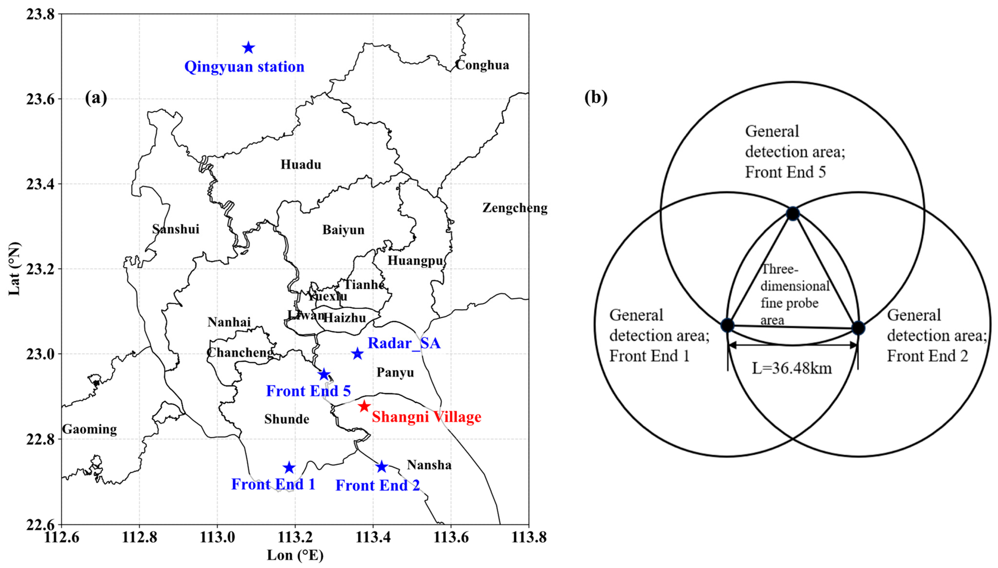
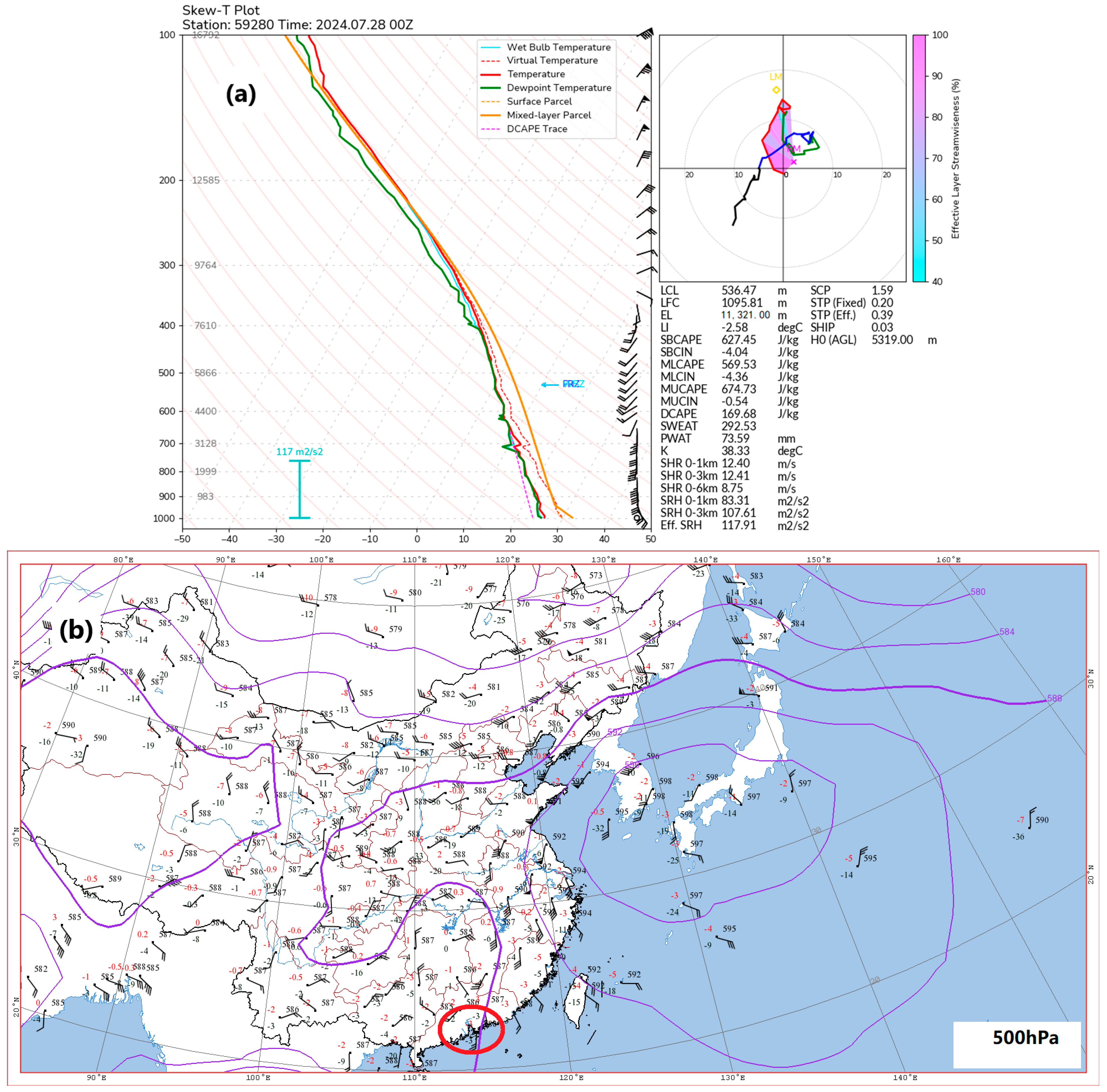
2.2.1. Weather Background

Around 00:24 on 28 July 2024, a tornado event occurred in Guangzhou, Guangdong Province, lasting 3 min, and it was associated with strong thunderstorm clouds.

Soundings from the Qingyuan sounding station (the closest to Foshan’s Nanhai District) at 00:00 on 28 July 2024 (Figure 3) show that, on that day, the subtropical high extended westwards to the South China coast. The southwest flow at its edge continuously transported hot and humid air (with a dew point above 25 °C) to the Pearl River Delta, providing ample moisture and energy for strong convection. On the morning of 28 July, Nansha District experienced consecutive high temperatures (with the previous day’s maximum exceeding 35 °C). Rapid ground-surface radiation heating created a super-adiabatic temperature gradient in the lower atmosphere (0–3 km). The lifting condensation level (LCL) was low at only 500 m, which is favourable for rapid thunderstorm development. Figure 2 also shows the high relative humidity that was recorded across all atmospheric layers, as well as the extremely low atmospheric stability and a K index of 38.33.

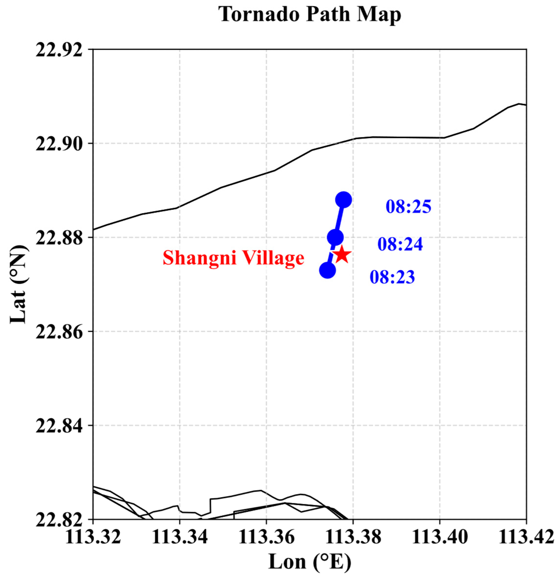
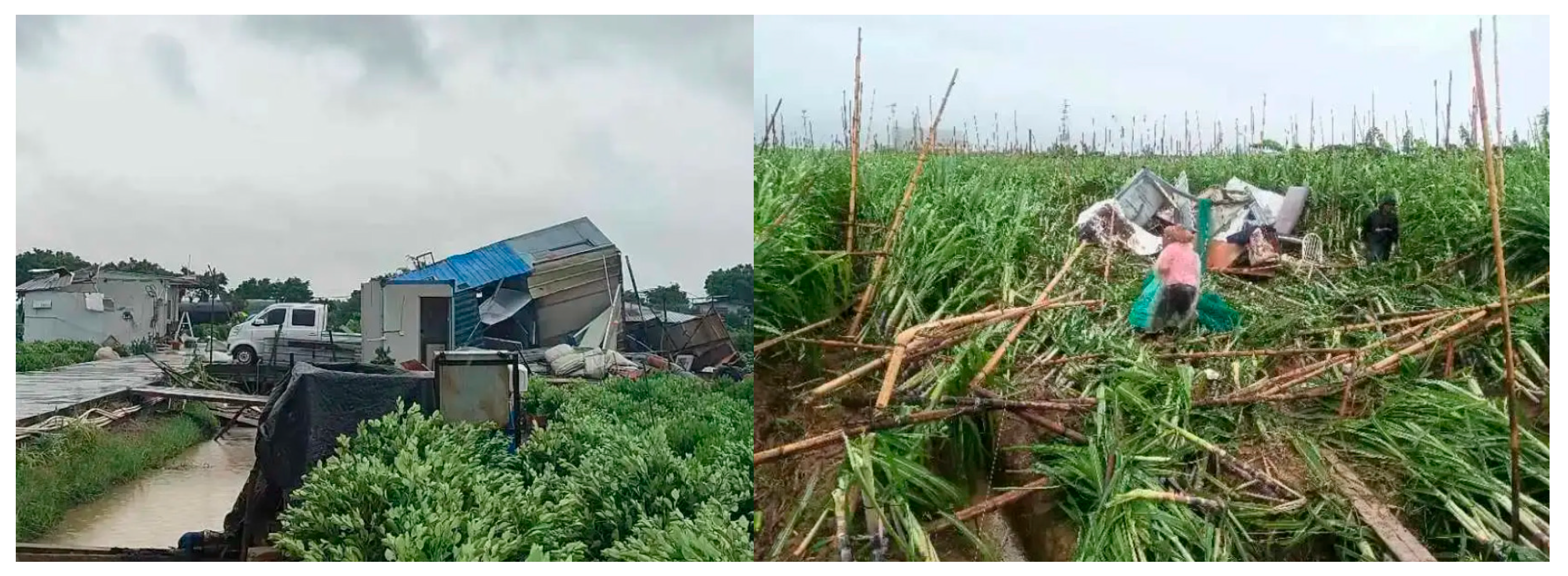
2.2.2. Tornado Observation

At 00:24 on 28 July 2024, a tornado struck near the farmland of Shangni Village, Lanhe Town, Nansha District, Guangzhou, Guangdong and it was triggered by a severe thunderstorm cloud mass.

Field investigation by Foshan’s meteorological department revealed the tornado moved from southwest to northeast. It caused the metal roofs of houses to be blown off and trees to be broken (Figure 4). The tornado’s path was about 1.9 km long and 180 m wide at most, and it lasted for 3 min. Rated as a medium-intensity tornado under Chinese national standards, it was equivalent to the Enhanced Fujita scale EF1.

2.3. Research Methods

2.3.1. Three-Dimensional Direct Synthesis Wind Field Algorithm

The direct synthesis wind field algorithm is relatively simple and is applicable when radial velocity measurements from three or more phased-array radar front ends are available. After performing quality control on the radial velocity data from each radar front end, the data are transformed into a common co-ordinate system and interpolated onto a Cartesian grid using a two-dimensional interpolation method. Specifically, nearest-neighbour interpolation—neglecting Earth’s curvature—is applied in the horizontal direction, while linear interpolation is used in the vertical direction. The horizontal resolution of the grid is 100 m × 100 m and the vertical resolution is 200 m.

A geocentric Cartesian co-ordinate system was adopted, with its origin at the Earth’s -axis pointing eastwards, the y-axis pointing northwards and the z-axis directed vertically upwards. Each radar array front end was located at co-ordinates ($x_i,y_i,z_i$), $i$ = 1, 2, 3 …, and any point in the 3D spatial domain was represented by co-ordinates ($x,y,z$). Let $V_i$ denote the radial velocity observed by the $i$-th radar front end. The wind vector at the spatial point ($x,y,z$) is expressed as ($u,v,w$), where $u,v$ and $w$ represent the wind components in the east–west, north–south and vertical directions, respectively. The vertical component $w$ refers to the particle vertical velocity, which includes both the vertical air motion and the terminal fall velocity of hydrometeors. The relationship between the three-dimensional wind field and the radial velocities measured by the three radar sub-arrays is governed by Equation (1):

$$V_i={\displaystyle \frac{u\left(x-x_i\right)}{R_i}}+{\displaystyle \frac{v\left(y-y_i\right)}{R_i}}+{\displaystyle \frac{w\left(z-z_i\right)}{R_i}}$$

(1)

where $R_i=\sqrt{{\left(x-x_i\right)}^2+{\left(y-y_i\right)}^2+{\left(z-z_i\right)}^2}$ is the Euclidean distance between each front end and the target point ($u,v,w$) can be solved. Therefore, the calculated $u$ and $v$ can be used to calculate vorticity and divergence. The direct synthesis method uses mathematical theory to solve a system of simultaneous equations to obtain ($u,v$ and $w$), which is relatively simple. Furthermore, the $V_i$ values obtained by multiple radar front ends are independent of each other and do not interfere with each other. Array radars have a very small time difference in observing the same point, resulting in relatively accurate synthetic wind fields.

2.3.2. Vorticity and Divergence

Horizontal vorticity (hereinafter referred to as vorticity) is an important physical quantity that characterises the rotational nature of atmospheric wind fields. It directly reflects the degree of rotation of vortices and is of great significance for the study of cyclonic weather, such as tornadoes. Based on the east–west ($U$) and north–south ($V$) horizontal vector wind speeds derived from the three-dimensional wind field inverted by array weather radar, vorticity can be calculated using Formula (2):

$$\xi ={\displaystyle \frac{\partial V}{\partial x}}-{\displaystyle \frac{\partial U}{\partial y}}$$

(2)

where ${\displaystyle \frac{\partial V}{\partial x}},{\displaystyle \frac{\partial U}{\partial y}}$ represent the rate of change in the north–south winds in the east–west direction and the rate of change in the east–west winds in the north–south direction, respectively.

Divergence is a physical quantity that reflects the strength of divergence and convergence in a flow field. Horizontal divergence describes the degree of divergence or convergence of a wind field in the horizontal direction. The magnitude of horizontal divergence D is calculated from the measured wind field on the same horizontal plane. Based on the east–west ($U$) and north–south ($V$) horizontal vector wind speeds derived from the three-dimensional wind field inverted by the array weather radar, the divergence can be calculated with the horizontal divergence given by Formula (3):

$$D={\displaystyle \frac{\partial U}{\partial x}}+{\displaystyle \frac{\partial V}{\partial y}}$$

(3)

where ${\displaystyle \frac{\partial U}{\partial x}},{\displaystyle \frac{\partial V}{\partial y}}$ represents the rate of change in east–west winds along the east–west direction and the rate of change in north–south winds along the north–south direction, respectively.

2.3.3. Vorticity Volume

Vorticity volume ($VV$) is the volume occupied by regions in a fluid where the vorticity exceeds a specific threshold. It is calculated using Formula (4):

$$VV={\displaystyle {\int }_V\theta \left(\Vert \xi \left(h_i\right)\Vert -{\xi }_{thresh}\right)}dV$$

(4)

where θ is the Heaviside step function, θ = 1, when the vorticity exceeds the threshold and θ = 0 otherwise; $\Vert \xi \left(h_i\right)\Vert$ is the vorticity modulus at a certain layer height; and ${\xi }_{thresh}$ is the set threshold. The vorticity volume utilised in this paper only calculates the volume occupied by eddies that exceed the vorticity threshold, where $V$ is the volume of the fluid region and $dV$ is a volume element.

2.4. Data Comparison and Validation

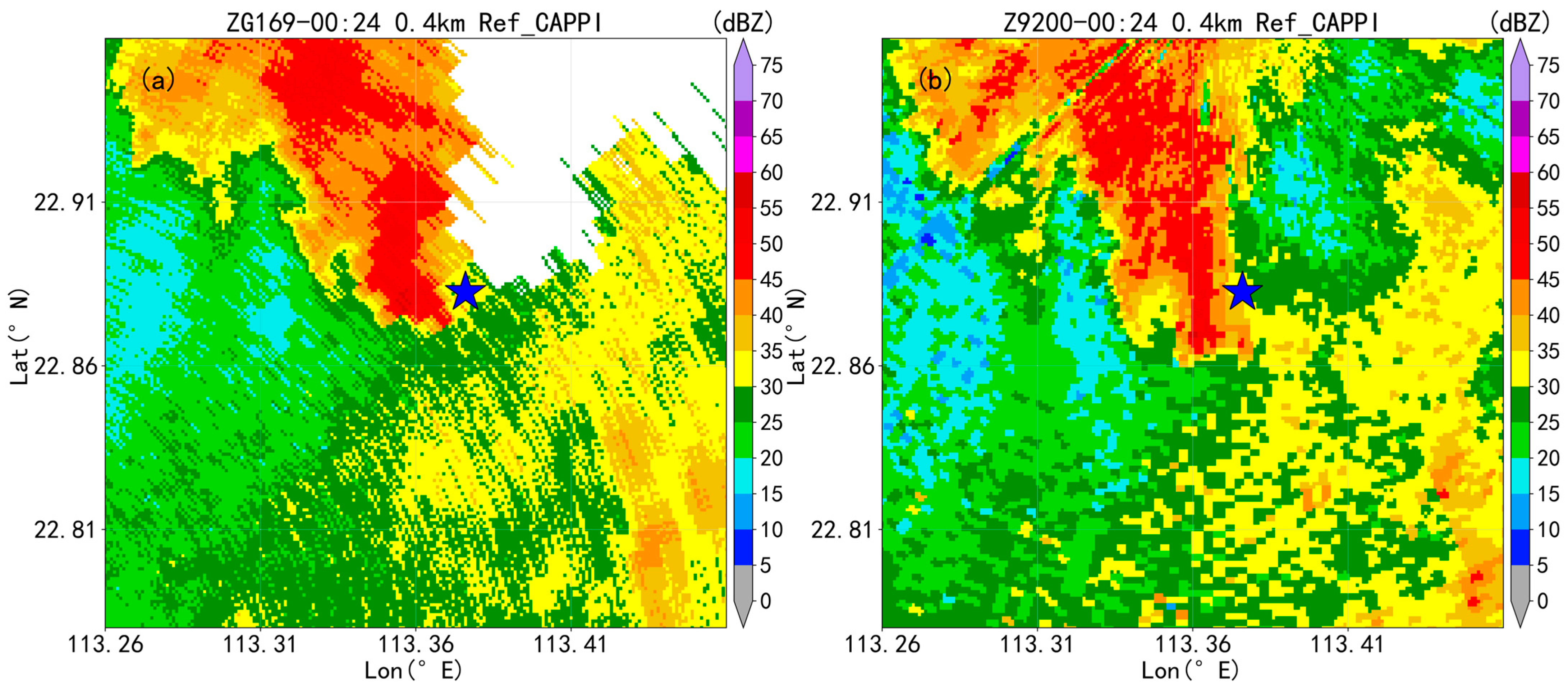
2.4.1. Echo Intensity Comparison

In monitoring severe convective weather, areas with echo intensity > 45 dBz are often regarded as strong echo areas [35], which are closely linked to weather such as heavy rain and hail. S-band radar scans from lower to higher elevations, taking around 6 min per volume scan. As the height increases, the time gap between lower- and upper-level data collection grows. To reduce interference from this time difference, lower-altitude detection data are preferred.

As shown in Figure 5, by comparing the reflectivity of the X-band phased array radar and the Guangzhou radar, it can be seen that the echo shapes and intensities detected by the two radars are consistent.

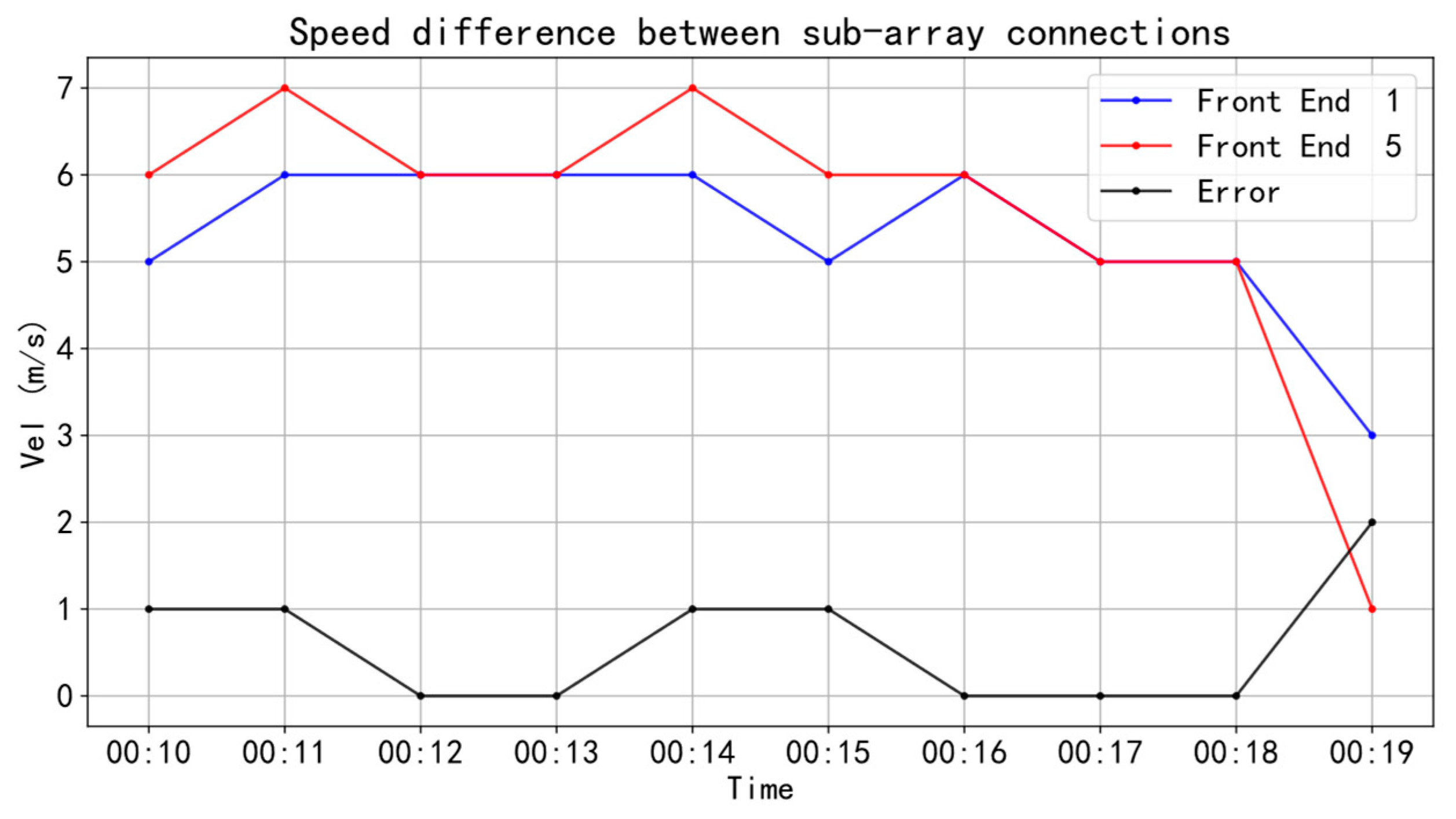
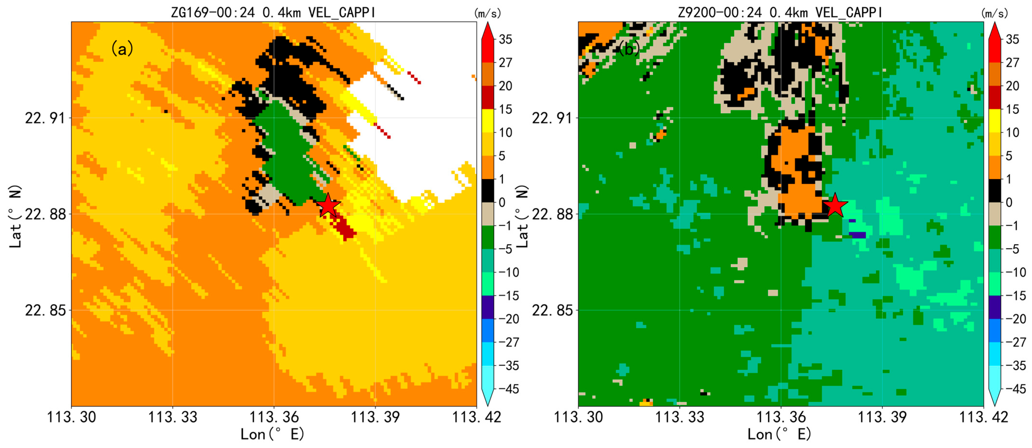
2.4.2. Radial Velocity Comparison

A radial velocity comparison between adjacent phased-array radar units should show correlations [27,28]. In theory, radial velocities at the midpoint of a line connecting adjacent units should be equal in magnitude but opposite in direction. To verify this, we focused on the radial velocities at the midpoints between adjacent units at a low elevation angle. Since ground clutter can significantly affect 0° elevation data, we instead used 1.5° elevation data.

As shown in Figure 6, taking the comparison between Front End 2 (Zhongshan Shaweiwei Station) and Front End 6 (Shunde San Gui Shan Station) as an example, we analysed the radial velocities at the midpoints of the line connecting these two fronts. We used data from 10 consecutive time points between 00:10 and 00:19 with a 1 min interval. The radial velocities from Front End 2 were inverted for comparison. The results showed that the radial velocities from Front End 2 and Front End 5 at each time point met the design requirement of being opposite in direction (i.e., numerical inversion). The maximum difference in the radial velocity values was 2 m/s, which satisfies the radial velocity consistency condition for verifying wind field rationality, as was proposed by Li Yu [34].

As shown in Figure 7, taking the radar data at 00:24 as an example, both radars showed distinct pairs of positive and negative radial velocities. The maximum positive and negative differences in the radial velocity pairs detected by both the X-band phased-array radar and the CINRAD/SA radar in Guangzhou were about 25 m/s.

3. Results

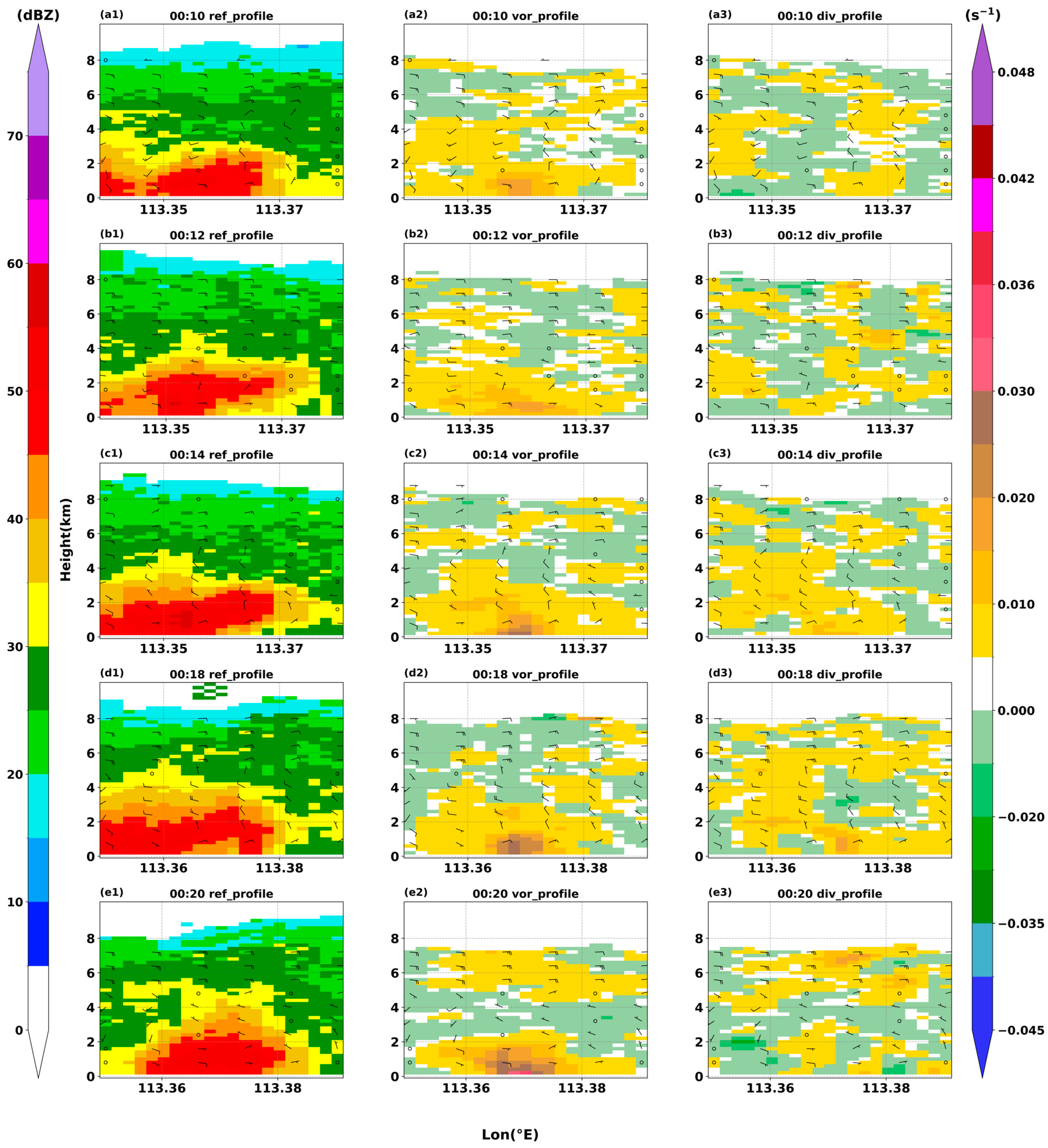
3.1. Tornado Genesis and Development Stages

On 28 July 2024, the X-band phased-array radar Front End 1 (Nansha Station) detected the following in its one-minute intensity CAPPI monitoring. At 00:10 (Figure 8a), arc-shaped echoes first appeared at the radar’s 62° azimuth (with true north as 0° azimuth), approximately 20 km from the radar centre. The intensity of the southwest strong echo mass was 45–55 dBz. By 00:12 (Figure 8b), arc-shaped echoes developed below a 2.5 km altitude at the radar’s 61° azimuth, also around 20 km from the radar centre. The southwest strong echo mass intensity reached 45–55 dBz, indicating a strengthening of the strong convection area. At 00:14 (Figure 8c), arc-shaped strong echoes with an intensity of 45–55 dBz appeared at the radar’s 56° azimuth, approximately 21 km from the radar centre. At 00:18 (Figure 8d,e), arc-shaped strong echoes with an intensity of 45–55 dBz were located at the radar’s 52° azimuth, about 22 km from the radar centre. Meanwhile, annular echoes with an intensity of 45–50 dBz emerged at a 0.6 km altitude. By 00:20 (Figure 8f), annular strong echoes appeared at the radar’s 51° azimuth, approximately 22.5 km from the radar centre. Arc-shaped strong echoes in the area still maintained an intensity of 45–55 dBz. Overall, the arc-shaped echoes moved northeast over time, and the echo hole continuously filled in.

This study utilised the X-band phased-array radar Front End 1, 2 and 5 to detect data, and it also employed the wind field synthesis algorithm to synthesise the wind field, divergence and vorticity during the tornado weather process. Figure 9 presents the wind field, intensity (four-front-end-merged echo), vorticity and divergence at 00:10, 00:12, 00:14, 00:18 and 00:20, respectively. It can be seen that the vortex position gradually moved northeast over time. Regarding echo characteristics, arc-shaped strong echoes emerged from 00:10 to 00:14 and they then evolved into annular strong echoes from 00:18 to 00:20, with a higher echo intensity on the southwest side. Echo intensity progressively increased from 00:10 to 00:20, peaking at 00:20 before subsiding. The wind speed rose from 00:10 to 00:20 and then stabilised at around 16 m/s. At 00:10, positive vorticity was present in the mid-layer of 0.2–1.0 km with vorticity values below 0.020 s⁻¹. From 00:14 to 00:20, positive vorticity occurred below 2.0 km and continued to strengthen. From 00:20 onwards, the wind field clearly formed a closed vortex. Divergence showed that the positive vorticity centre was positive (divergence) on the right side of the tornado’s movement direction and negative (convergence) on the left side.

Figure 10 presents the longitude-based profiles of the intensity, vorticity and divergence along the positive vorticity centre, with

Table 2. The specific coordinates of the vortex from 00:10 to 00:30 on 28 July 2024.

Time	Vortex Position
00:10	(113.3602°E, 22.820°N)
00:12	(113.3621°E, 22.828°N)
00:14	(113.3640°E, 22.835°N)
00:16	(113.3661°E, 22.843°N)
00:18	(113.3679°E, 22.850°N)
00:20	(113.3702°E, 22.858°N)
00:23	(113.3741°E, 22.873°N)
00:24	(113.3759°E, 22.880°N)
00:25	(113.3778°E, 22.888°N)
00:26	(113.3800°E, 22.895°N)
00:28	(113.3819°E, 22.902°N)
00:30	(113.3837°E, 22.910°N)

indicating the specific longitudes of the profiles. It shows that the high-intensity echoes (>45 dBz) mainly occurred between 0 and 4 km, and their area gradually decreased over time. A weak echo area emerged near the tornado centre at the lower level, while strong echoes appeared on both sides and at the upper level. The south side of the tornado centre had a downwards vertical velocity, and the north side had an upwards vertical velocity. The positive vorticity centre stayed at the lower level, with its vorticity value gradually rising to 0.035 s⁻¹ and then gradually reaching the ground. Divergence showed negative (convergence) values on the south side of the positive vorticity centre and positive (divergence) values on the north side.

Figure 11 presents the latitude-based profiles of the intensity, vorticity and divergence along the positive vorticity centre. The strong echoes mainly occurred below 2 km and their area gradually decreased over time, with stronger echoes on the west side of the tornado centre. The west side of the tornado centre had an upwards vertical velocity, and the east side had a downwards vertical velocity. The vorticity value gradually increased to 0.039 s⁻¹. Divergence showed positive (divergence) values on the west side of the positive vorticity centre and negative (convergence) values on the east side.

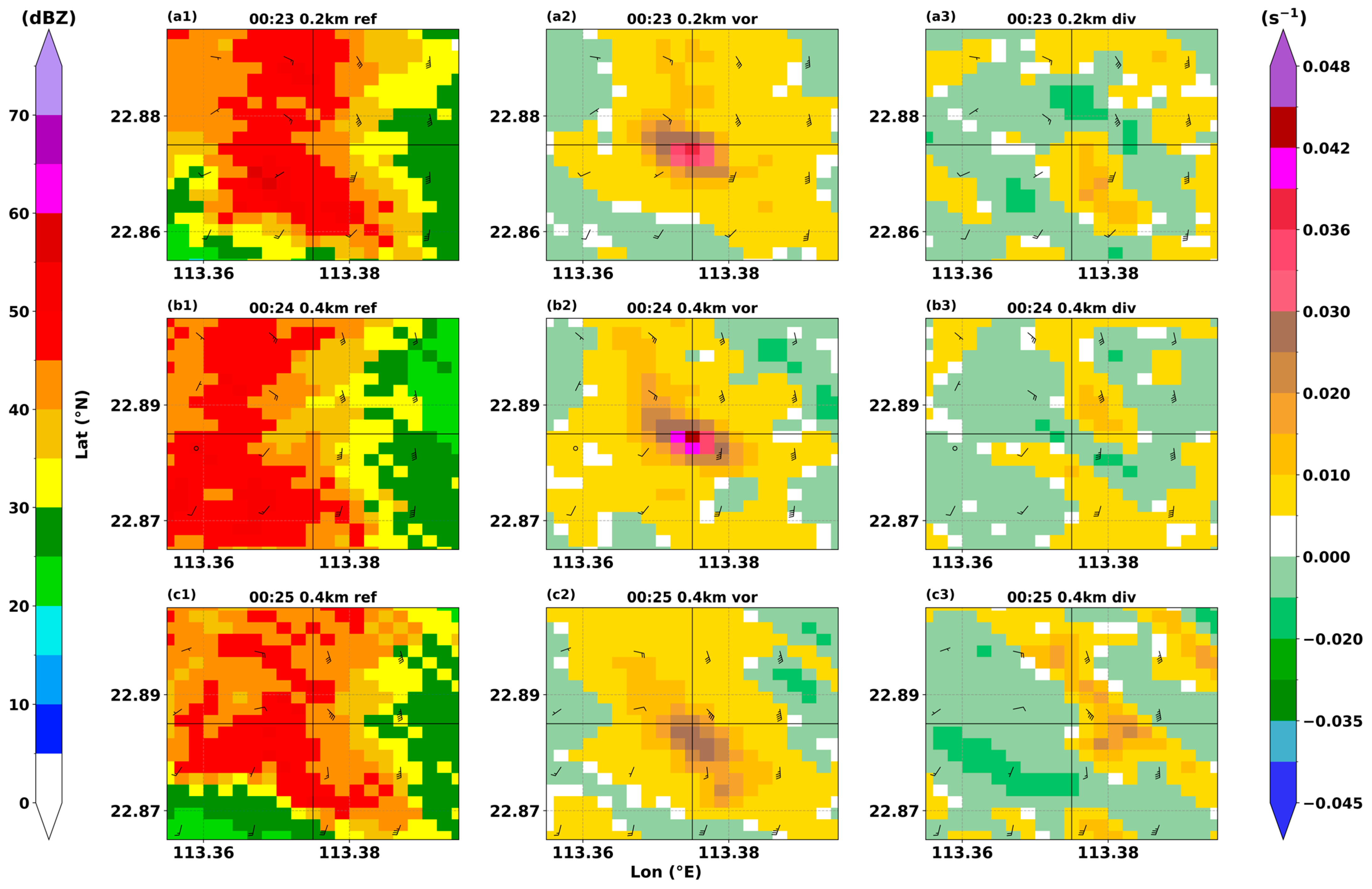
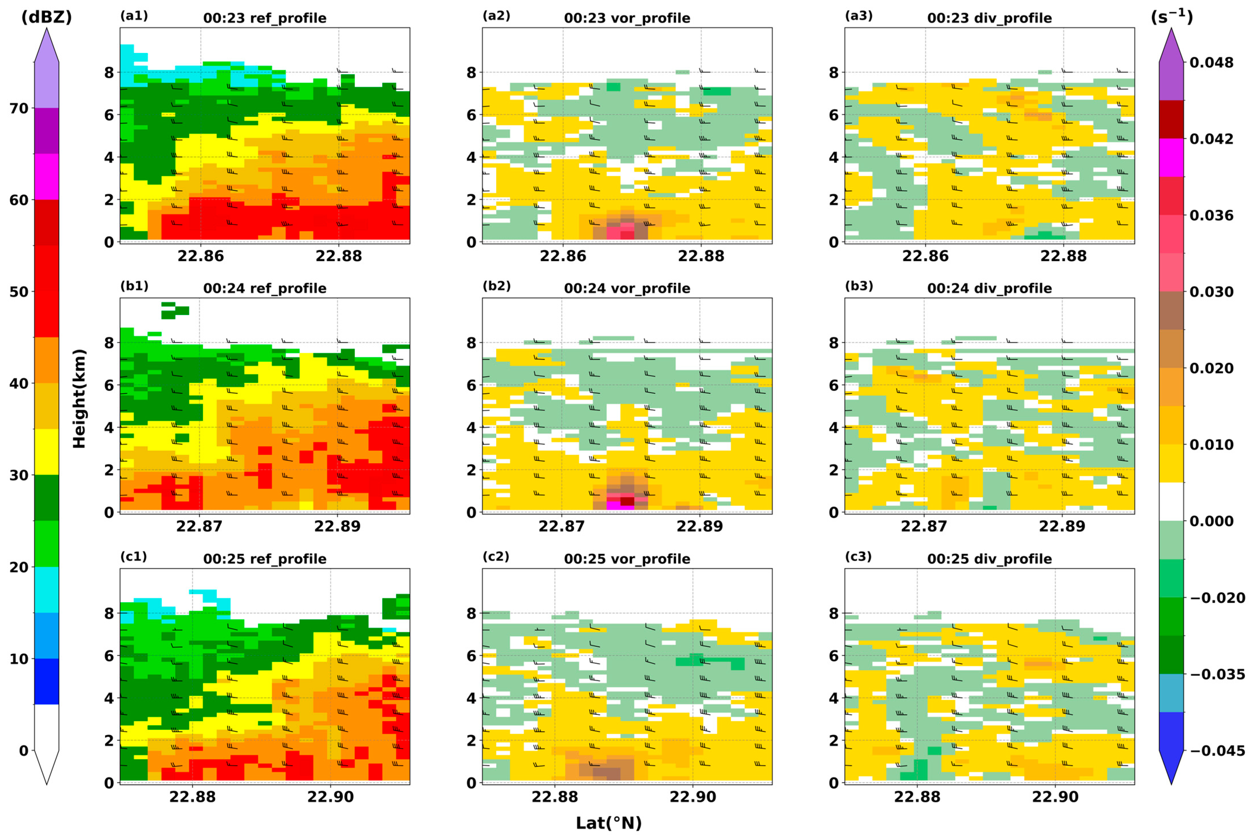
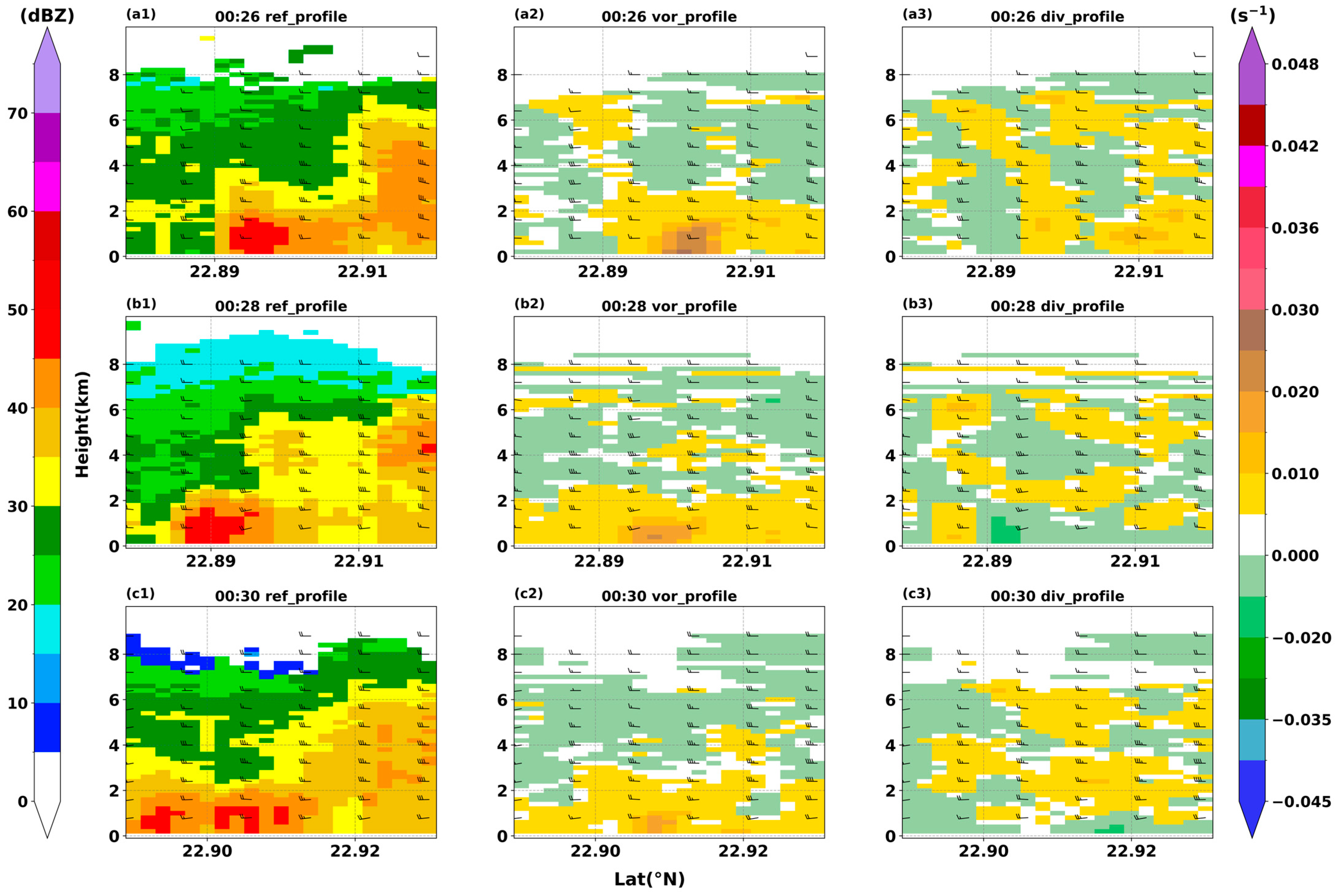
3.2. Tornado Mature Stage

The intensity CAPPI from the X-band phased-array radar Front End 1 (Nansha Station) at 00:24 (Figure 12) showed a distinct annular echo at the radar’s 47° azimuth, which was about 24 km from the radar centre, with an intensity of approximately 45–50 dBZ.

Figure 13 presents the wind field, intensity (four-front-end-merged echo) vorticity and divergence at 00:23, 00:24 and 00:25. The vortex continued to move northeast from the southwest over time. In terms of echo characteristics, distinct arc-shaped echoes emerged on the left side of the vortex, with echo intensity reaching 45–50 dBZ on the southwest side of the tornado’s movement direction. Positive vorticity was observed between 0.2 and 2.0 km in altitude, with a maximum value of 0.042 s⁻¹, which was predominantly within the mid-lower layer of 0.2–1.0 km. Divergence showed positive (divergence) values on the right side of the tornado’s movement direction and negative (convergence) values on the left side.

Figure 14 displays the longitude-based profiles of the intensity, vorticity and divergence along the positive vorticity centre. The profiles show strong echoes (>45 dBZ) mainly concentrated between 0 and 4 km, with a weak echo column at the tornado centre and stronger echoes on both sides. The positive vorticity centre was located between 0 and 2 km and was surface-based, with a vorticity magnitude of 0.042 s⁻¹. Divergence showed negative (convergence) values at the positive vorticity centre and positive (divergence) values on both sides.

Figure 15 presents the latitude-based profiles of the intensity, vorticity and divergence along the positive vorticity centre. The profiles show strong echoes (>45 dBZ) mainly concentrated between 0 and 2 km, primarily on the west side of the tornado centre. The west side of the tornado centre had an upwards vertical velocity, and the east side had a downwards vertical velocity. The positive vorticity centre was located between 0 and 2 km with a maximum value of 0.042 s⁻¹. Divergence showed negative (convergence) values on the west side of the positive vorticity centre and positive (divergence) values on the east side.

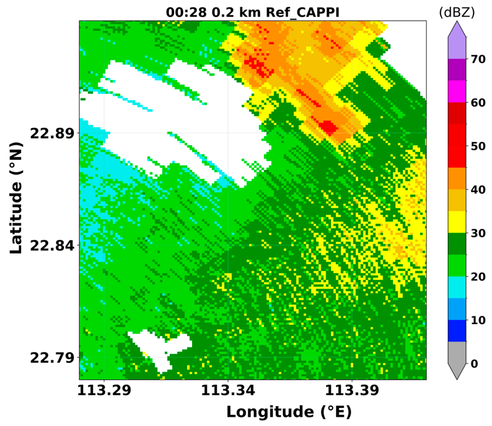
3.3. Tornado Dissipation Stage

The intensity CAPPI from the X-band phased-array radar Front End 1 (Nansha Station) showed that, at 00:28 (Figure 16), the echo characteristics gradually disappeared and the echo intensity weakened.

Figure 17 presents the wind field, intensity (three-front-end-merged echo) vorticity and divergence at 00:26, 00:28 and 00:30. The vortex continued to move northeast. At 00:26, the vortex shrank, and the vorticity decreased, indicating tornado dissipation. By 00:30, the vorticity had nearly vanished. Divergence showed positive (divergence) values on the right side of the tornado’s path and negative (convergence) values on the left.

Figure 18 shows the longitude-based profiles of the intensity, vorticity and divergence along the positive vorticity centre. Echo intensity diminished over time. The positive vorticity centre was below 2.0 km, with vorticity decreasing below 0.015 s⁻¹. At 00:26, the tornado vortex centre showed negative (convergence) values, with positive (divergence) values on both sides. From 00:28 onwards, low-level divergence became negative (convergence), indicating tornado dissipation.

Figure 19 displays the latitude-based profiles of the intensity, vorticity and divergence along the positive vorticity centre, with specific latitudes for each time in Table 2. Echo intensity gradually disappeared. The positive vorticity centre was below 2.0 km, with vorticity decreasing over time. The west side of the tornado vortex centre had upwards vertical velocity, and the east side had downwards vertical velocity. The tornado vortex centre showed negative (convergence) values, with positive (divergence) values on both sides, indicating tornado dissipation.

4. Discussion

4.1. Initial Construction of Vorticity Volume

Vorticity, indicating the local rotation intensity and direction of a fluid, typically aligns with the vortex centre at its maximum. To enhance the analysis of the vortex structure’s overall rotation and spatial distribution, the new parameter “vorticity volume” is introduced. This improves the practicality and versatility of vorticity in real-world applications.

In Formula (4), the threshold is particularly important for calculating the vorticity volume. Here, the threshold refers to the critical criterion value ${\xi }_{\begin{array}{c}thresh\end{array}}$ obtained through calculation, which defines the significant vortex region through the operational condition $\xi \ge {\xi }_{thresh}$. Its necessity is based on the following core reasons.

• Addressing the ambiguity of vortex boundaries: Fluid vorticity fields exhibit continuity and there are no absolute vortex boundaries. Thresholds introduce intensity thresholds to separate physically significant rotational structures from background vorticity and weak vorticity noise, thereby objectively defining the spatial extent of vortices.
• Quantifying vortex-dominated regions: The calculation of vorticity volume depends on the identification of significant vortex regions.
• Suppressing non-physical interference: The threshold can filter out discrete errors, maximising the assurance that the extracted vortex structures reflect real physical processes rather than numerical counterfeit.
• The threshold is calculated using a method based on the vortex core method combined with statistical analysis. The specific steps are as follows: Calculate the three-dimensional vorticity field using three-dimensional wind field data, and then calculate the vorticity magnitude field (each grid point has only one vorticity magnitude value). Iterate through all the time steps of the vorticity magnitude values find the median value, and then set it as the environmental vorticity.
• For each time step, iterate through the vorticity magnitude field at each layer height to identify vorticity cores; i.e., local maximum points (determine whether the point is the maximum value within its neighbourhood (9 × 9)).
• Count the number of vorticity values ${\xi }_i\left(i=1,2,...,N\right)$ that are adjacent to the vortex core and greater than the environmental vorticity at all time steps and heights.
• Calculate the root mean square of all qualified vorticity values to obtain the threshold, as shown in Formula (5):

  $${\xi }_{thresh}=\sqrt{{\displaystyle \frac{1}{N}}{\displaystyle \sum _{i=1}^N{\xi }_i^2}}$$

  (5)

After obtaining the threshold, calculate the vorticity volume using the following steps:

• Calculate the vorticity field using three-dimensional wind field data. Based on the obtained threshold ${\xi }_{\begin{array}{c}thresh\end{array}}$, apply a step function to determine whether the vorticity of the vortex exceeds the threshold, thereby binarising the vorticity field.
• Using the connected domain (eight-connected) method, identify the connected domains at each height layer of the vortex and count the number of grid points in the connected domains that meet the conditions at each height layer of the vortex.
• To ensure vertical continuity, first calculate the area of the connected domains that meet the conditions at each height level. Based on the resolution of the three-dimensional grid point data (100 m × 100 m × 200 m), the area is equal to the number of grid points in the connected domain multiplied by 10,000 m².
• Use the common area ratio method to ensure vertical continuity. The common area ratio formula is as follows:

$$\alpha ={\displaystyle \frac{A_C}{\min \left(A_1,A_2\right)}}$$

(6)

where $A_C=A_1\cap A_2$ is the area of overlap between two connected domain units.

• Finally, the vorticity volume is equal to the total number of grid points multiplied by the unit volume (i.e., total number of grid points × 2,000,000 m³).

We made the following comparisons to verify the accuracy of the vortex volume calculation results (using 00:24 as an example). As shown in Figure 20, according to the above steps, at 00:24, the vorticity area at each altitude layer corresponded to the area of the connected domain (the figure shows the number of grid points in the connected domain, which was compared after multiplying the number by the horizontal resolution and converting the units).

The following is an analysis of the vorticity volume of the two tornadoes that occurred on 28 July 2024, and 18 June 2022 (19 June 2022 BJT).

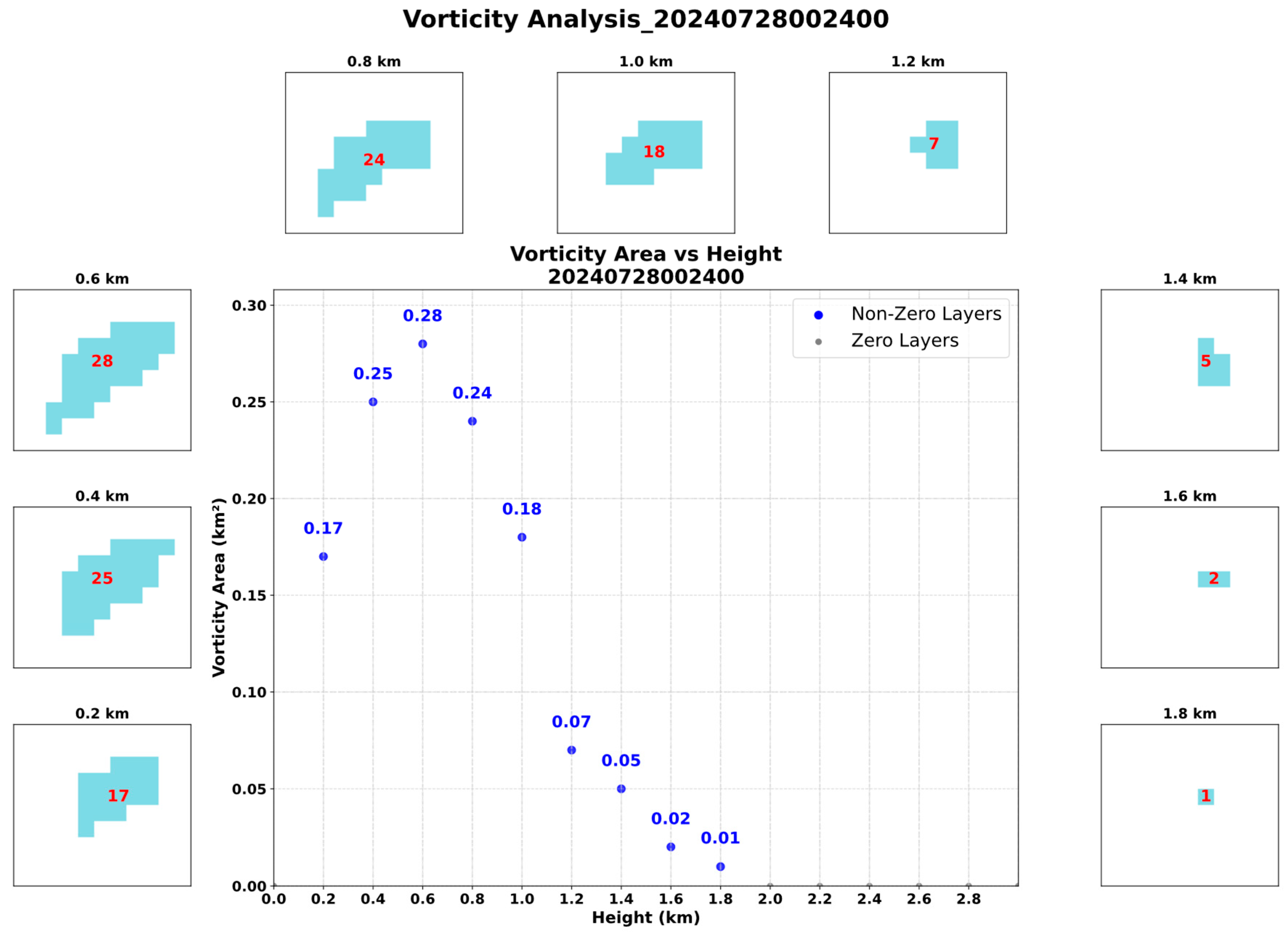
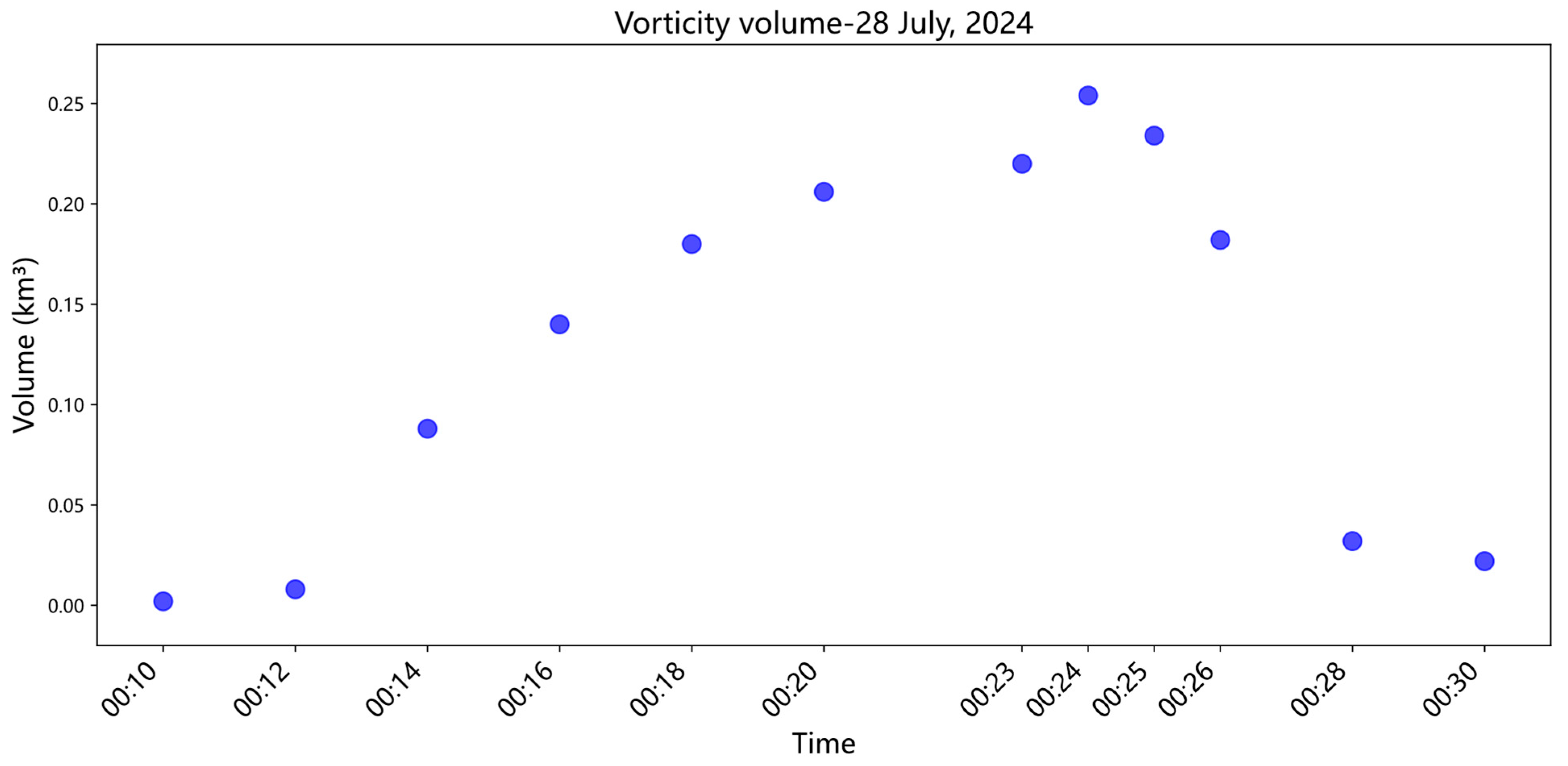
4.2. Analysis and Discussion of the Vorticity Volume

For the 28 July 2024, tornado, according to the above threshold calculation method, the threshold was set at 0.018 s⁻¹ and only the volume exceeding this vorticity threshold was calculated. Before calculating the vorticity volume, the vorticity area at different height layers for each time point was analysed. Figure 21 shows the vorticity area at each height layer for each time point, reflecting the size of the vorticity area exceeding the threshold at each height and time. From 00:10 to 00:12, the vorticity area at all height layers began to increase slightly below 1.0 km. From 00:14 to 00:16, a significant increase occurred below 0.8 km, with the maximum vorticity area exceeding 0.15 km². From 00:18 to 00:24, the vorticity area at all height layers further increased, peaking at 0.28 km² at 00:24. Although the maxima at 00:20 and 00:23 were slightly lower than at 00:18, the overall vorticity area still increased over time. From 00:25 to 00:30, the vorticity area at all height layers decreased, with a marked decline from 00:26 to 00:28 until the tornado dissipated.

As shown in Figure 22, from 00:10 to 00:24, the tornado’s vorticity volume gradually increased, with a significant upwards trend from 00:12 to 00:20. It peaked at 00:24 and then sharply decreased until the tornado dissipated.

To analyse the distribution patterns of the vorticity volume during tornado development, this study additionally introduced a tornado event that occurred in Guangzhou City, Guangdong Province, on 19 June 2022 for supplementary analysis. For the 18 June 2022 tornado, according to the above threshold calculation method, the threshold was set at 0.030 s⁻¹, and only the volume exceeding this vorticity threshold was calculated. Before calculating the vorticity volume, the variation in vorticity area at different height layers for each time point was analysed. Figure 23 shows the vorticity area at each height layer for each time point, reflecting the size of the vorticity area exceeding the threshold at each height and time. From 22:46 to 22:52, there was a slight increase in vorticity area at all height layers, mainly between 0.2 km and 1.2 km. At 23:00, the vorticity area at all height layers increased rapidly, with a maximum value of 0.20 km² at 0.6 km. From 23:10 to 23:22, the maximum vorticity area at 23:10 decreased somewhat, with larger values concentrated between 1.0 km and 2.0 km. From 23:16 to 23:21, the vorticity area increased between 0.2 km and 1.0 km. At 23:22, the maximum vorticity area reached a peak of 0.24 km² at 0.2 km. After 23:22, the vorticity area decreased significantly and, by 23:32, the vorticity area at all height layers dropped to zero.

As shown in Figure 24, from 22:40 to 23:22, the tornado’s vorticity volume gradually increased overall, with a marked upwards trend after 23:05. It peaked at 23:22 and then sharply decreased until the tornado dissipated. This variation in the vorticity volume aligned well with the entire development process of the tornado, as per Wang Ruifeng’s [32] analysis.

5. Conclusions

This study analysed the echo intensity, dynamic conditions and mesoscale structural characteristics of an EF1 tornado in Guangzhou, Guangdong, on 28 July 2024. Using high-resolution data from an X-band phased-array radar, we synthesised the 3D wind field to investigate the evolution of the supercell storm and its internal cyclone. After systematic quality control of the radar data, validation with the Guangzhou S-band radar data and comparison among radar fronts, we confirmed the accuracy and completeness of the radial velocity data, deeming the synthesised wind field reliable for analysing the tornado process.

The key conclusions are as follows:

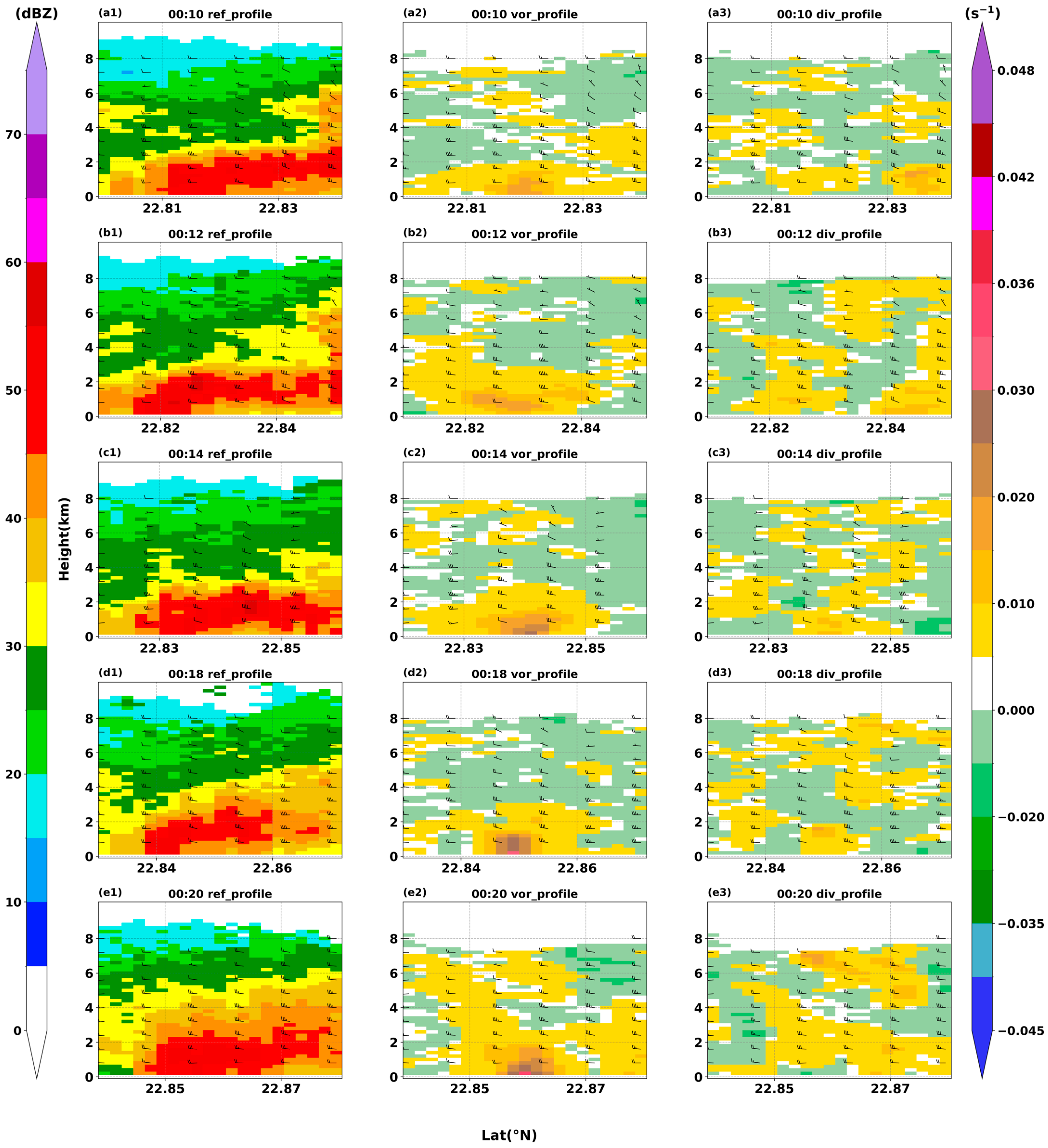
• The tornado displayed classic supercell features, such as hook echoes and a weak echo centre. During its early development, arc-shaped strong echoes appeared about 14 min prior, with annular echoes emerging at 00:18, mainly between 0 and 4 km. A weak echo area formed at the tornado centre. After 00:24 (tornado occurrence), the annular echoes gradually reverted to being arc-shaped, and echo features eventually disappeared as the tornado dissipated.
• The tornado vortex moved northeast from the southwest. Before 00:20, vorticity was low but increasing. From 00:10 to 00:24, vortex depth and vorticity grew, peaking at 00:24, which is when the positive vorticity centre reached the ground. After 00:25, vorticity declined, indicating tornado dissipation and, by 00:30, it nearly vanished. The positive vorticity centre showed divergence on the tornado’s movement side and convergence on the opposite side.
• To assess the vortex structure’s overall rotation and distribution, this study introduced vorticity volume, analysing two tornadoes (28 July 2024 and 18 June 2022). The total vorticity area across height layers gradually increased in the tornado’s early stage, peaked at maturity and then rapidly decreased. Similarly, vorticity volume rose from the initial stage, peaked at tornado occurrence and then decayed until dissipation, closely aligning with the tornado life cycle.

Although this study revealed patterns in the tornado’s development using the X-band array radar and vorticity volume analysis, it has limitations due to the lack of a larger tornado sample for statistical validation. Future research will build on this work to further explore tornado dynamics.

References

1. Diao, X.; Meng, X.; Zhang, L.; Ren, Z.; Zhao, H. Analysis of microscale vortex signature and early warning capability of tornadoes in the circulations of Typhoon YAGI and RUMBIA. J. Mar. Meteorol. 2019, 39, 19–28. [Google Scholar]
2. Brotzge, J.; Donner, W. The Tornado Warning Process: A Review of Current Research, Challenges, and Opportunities. Bull. Am. Meteorol. Soc. 2013, 94, 1715–1733. [Google Scholar] [CrossRef]
3. Squitieri, B.J.; Wade, A.R.; Jirak, I.L. A historical overview on the science of derechos: Part I: Identification, Climatology, and Societal Impacts. Bull. Am. Meteorol. Soc. 2023, 104, E1709–E1733. [Google Scholar] [CrossRef]
4. Crum, T.D.; Alberty, R.L. The WSR-88D and the WSR-88D operational support facility. Bull. Am. Meteorol. Soc. 1993, 74, 1669–1688. [Google Scholar] [CrossRef]
5. Crum, T.D.; Saffle, R.E.; Wilson, J.W. An update on the NEXRAD program and future WSR-88D support to operations. Weather Forecast. 1998, 13, 253–262. [Google Scholar] [CrossRef]
6. Berkowitz, D.S.; Schultz, J.A.; Vasiloff, S.; Elmore, K.L.; Payne, C.D.; Boettcher, J.B. Status of Dual Pol QPE in The WSR-88D Network. Am. Meteorol. Soc. 2013. [Google Scholar]
7. Ryzhkov, A.V.; Schuur, T.J.; Burgess, D.W.; Zrnic, D.S. Polarimetric tornado detection. J. Appl. Meteorol. 2005, 44, 557–570. [Google Scholar] [CrossRef]
8. Bluestein, H.B. Severe Convective Storms and Tornadoes; Springer: Berlin/Heidelberg, Germany, 2013; Volume 10, pp. 973–978. [Google Scholar]
9. Lemon, L.R.; Doswell, C.A., III. Severe thunderstorm evolution and mesocyclone structure as related to tornadogenesis. Mon. Weather Rev. 1979, 107, 1184–1197. [Google Scholar] [CrossRef]
10. Trapp, R.J.; Mitchell, E.D.; Tipton, G.A.; Effertz, D.W.; Watson, A.I.; Andra, D.L.; Magsig, M.A. Descending and nondescending tornadic vortex signatures detected by WSR-88Ds. Weather Forecast. 1999, 14, 625–639. [Google Scholar] [CrossRef]
11. Anderson-Frey, A.K.; Richardson, Y.P.; Dean, A.R.; Thompson, R.L.; Smith, B.T. Investigation of near-storm environments for tornado events and warnings. Weather Forecast. 2016, 31, 1771–1790. [Google Scholar] [CrossRef]
12. Wei, W.; Zhao, Y. The characteristics of Tornadoes in China. Meteorol. Mon. 1995, 21, 36–40. [Google Scholar]
13. Zhang, G.; Li, Y.; Jiang, J.; Chang, X.; Huo, Z.; Zhong, X.; Guo, B.; Jia, K. Characteristic Analysis of EF3 Strong Tornado Induced by Multiple Supercell Storms. Meteorol. Mon. 2023, 49, 1315–1327. [Google Scholar]
14. Liu, J.; Zhu, J.; Wei, D.; Song, Z.; Lu, H.; Zhou, H. Doppler Weather Radar Typical Characteristics of the 3 July 2007 Tianchang Supercell Tornado. Meteorol. Mon. 2009, 35, 32–39. [Google Scholar]
15. Song, Z.; Liu, J.; Zhang, J.; Lu, H.; Xiang, Y. Analysis of a severe Tornado in lingbi county with Doppler radar fuyang CINRAD/SA’s products. J. Meteorol. Sci. 2006, 26, 689–695. [Google Scholar]
16. Yu, X. Detection and Warnings of Severe Convection with Doppler Weather Radar. Adv. Meteorol. Sci. Technol. 2011, 1, 31–41. [Google Scholar]
17. Brooks, H.E.; Doswell, C.A.; Kay, M.P. Climatological estimates of local daily tornado probability for the United States. Weather Forecast. 2003, 18, 626–640. [Google Scholar] [CrossRef]
18. Hu, Y.; Kang, J.; Xie, Y.; Wang, C.; Sun, Z. Preliminary Analysis on the Cause of Tornadoe on July 3rd 2007. J. Anhui Agric. Sci. 2008, 36, 11936–11939. [Google Scholar]
19. Wu, F.; Yu, X.; Zhang, Z.; Zhou, X.; Wei, Y. A study of the environmental conditions and radar echo characteristics of the supercell-storms in northern Jiangsu. Acta Meteorol. Sinica 2013, 71, 209–227. [Google Scholar]
20. Zhou, H. Observations of 23 June 2016 EF4 tornado supercell thunderstorm mesoscale structure in Funing county, Jiangsu province. Chin. J. Geophys. 2018, 61, 3617–3639. (In Chinese) [Google Scholar]
21. Gu, Y.; Sun, J.; Chu, H. Analyses of Characteristics on A Super Tornado in Funing, Jiangsu Province in June, 2016. J. Ocean Univ. China 2018, 48, 11–21. [Google Scholar]
22. Noda, A.T.; Niino, H. A Numerical Investigation of a Supercell Tornado: Genesis and Vorticity Budget. J. Meteorol. Soc. Japan. Ser. II 2010, 88, 135–159. [Google Scholar] [CrossRef]
23. Fischer, J.; Dahl, J.M.L. Transition of Near-Ground Vorticity Dynamics during Tornadogenesis. J. Atmos. Sci. 2022, 79, 467–483. [Google Scholar] [CrossRef]
24. French, M.M.; Bluestein, H.B.; PopStefanija, I.; Baldi, C.A.; Bluth, R.T. Mobile, Phased-Array, Doppler Radar Observations of Tornadoes at X Band. Mon. Weather Rev. 2014, 142, 1010–1036. [Google Scholar] [CrossRef]
25. Kuster, C.M.; Heinselman, P.L.; Austin, M. 31 May 2013 El Reno Tornadoes: Advantages of Rapid-Scan Phased-Array Radar Data from a Warning Forecaster’s Perspective. Weather Forecast. 2015, 30, 933–956. [Google Scholar] [CrossRef]
26. Ma, S.; Chen, H.; Wang, G.; Zhen, X.; Xu, X.; Li, S. Design and initial implementation of array weather radar. J. Appl. Meteorol. Sci. 2019, 30, 1–12. [Google Scholar]
27. Li, Y.; Ma, S.; Yang, L.; Zhen, X.; Qiao, D. Wind field verification for array weather radar at Changsha Airport. J. Appl. Meteorol. Sci. 2020, 31, 681–693. [Google Scholar]
28. Xiao, J.; Yang, L.; Yu, X.; Ma, S.; Li, C.; Qiao, D. Analysis of Short-Time Severe Rainfall on 4 September 2020 Detected by Phased Array Radar in Foshan. Meteorol. Mon. 2022, 48, 826–839. [Google Scholar]
29. Zhen, X.; Ma, S.; Chen, H.; Wang, G.; Xu, X.; Li, S. A New X-band Weather Radar System with Distributed Phased-Array Front-ends: Development and Preliminary Observation Results. Adv. Atmos. Sci. 2022, 39, 386–402. [Google Scholar] [CrossRef]
30. Zhang, Y.; Bai, L.; Meng, Z.; Chen, B.; Tian, C.; Fu, P. Rapid-Scan and Polarimetric Phased-Array Radar Observations of a Tornado in the Pearl River Estuary. J. Trop. Meteorol. 2021, 27, 81–86. [Google Scholar]
31. Zhi, J.; Bai, L.; Huang, X.; Cai, K.; Zhang, J.; Li, Z.; Huang, S. Observation of the 19 June 2022 Tornado by X-Band Polarimetric Phased Array Radar in Foshan, Guangdong. J. Trop. Meteorol. 2024, 40, 297–312. [Google Scholar]
32. Wang, R. A Study of Tornadoes Based on Array Weather Radar Detection. Master’s thesis, Chengdu University of Information Technology, Chengdu, China, 2024. [Google Scholar]
33. Potvin, C.K.; Betten, D.; Wicker, L.J.; Elmore, K.L.; Biggerstaff, M.I. 3DVAR versus traditional dual-Doppler wind retrievals of a simulated supercell thunderstorm. Mon. Weather Rev. 2012, 140, 3487–3494. [Google Scholar] [CrossRef]
34. Li, Y.; Ma, S.; Yang, L.; Zhen, X.; Qiao, D. Sensitivity analysis on Data Time Difference for wind fields synthesis of array weather radar. SOLA 2020, 16, 252–258. [Google Scholar] [CrossRef]
35. Han, G. Statistical analysis of the evolution of strong echoes. Meteorol. Mon. 2008, 115–117. [Google Scholar]
Figure 1. (a) Layout of the Guangzhou CINRAD/SA radar and the Foshan Array Weather Radar. (The blue pentagram represents radar stations and weather stations, while red represents tornado locations.) (b) Examples of the three transceiver front end detection areas.
Remotesensing 17 02615 g001
Figure 2. Tornado movement path. (The red pentagram indicates the location of the village where the tornado occurred, while the blue dots represent the tornado’s position at different times and illustrate its movement path.)
Remotesensing 17 02615 g002
Figure 3. (a) The Qingyuan Sounding Station 07.28 00:00 sounding chart; (b) upper-level sounding data at 500 hPa (the red oval marks the location where the tornado occurred).
Remotesensing 17 02615 g003
Figure 4. Damage caused by the tornado on 28 July 2024.
Remotesensing 17 02615 g004
Figure 5. Radar intensity comparison conducted on 28 July 2024, at 00:24: (a) Front End 1 (ZG169) at a 0.4 km height echo intensity CAPPI; (b) Guangzhou Radar at a 0.4 km height echo intensity CAPPI. (The blue pentagram in the figure represents the location of the tornado. The white areas in Figure a are caused by the attenuation of radar electromagnetic waves after encountering strong echoes.)
Remotesensing 17 02615 g005
Figure 6. Radial velocity comparison at the midpoint of the front line from 00:10 to 00:19 on 28 July 2024. In the figure, the blue line represents the radial velocity of Front End 1, the red line represents the opposite of the radial velocity of Front End 5, and the black line represents the absolute value of the velocity difference.
Remotesensing 17 02615 g006
Figure 7. Comparison of the radial velocities of radars at 00:24: (a) Front End 1 (ZG169) radial velocity CAPPI at a 0.4 km altitude. (b) Guangzhou radar radial velocity CAPPI at a 0.4 km altitude. (The red pentagram in the figure represents the location of the tornado. The white areas in Figure a are caused by the attenuation of the intensity in that area, resulting in invalid radial velocities in the corresponding areas.)
Remotesensing 17 02615 g007
Figure 8. Typical altitude echo intensity maps: (a) CAPPI at 0.2 km at 00:10; (b) CAPPI at 0.2 km at 00:12; (c) CAPPI at 0.2 km at 00:14; (d) CAPPI at 0.2 km at 00:18; (e) CAPPI at 0.6 km at 00:18; and (f) CAPPI at 0.2 km at 00:20. (The white areas in the figure are caused by the attenuation of radar electromagnetic waves after encountering strong echoes.)
Remotesensing 17 02615 g008
Figure 9. The horizontal wind field and intensity (left), vorticity (middle), and divergence (right): (a1a3) 00:10; (b1b3) 00:12; (c1c3) 00:14; (d1d3) 00:18; and (e1e3) 00:20.
Remotesensing 17 02615 g009
Figure 10. Longitude profiles of the wind field and intensity (left), vorticity (middle) and divergence (right): (a1a3) 00:10; (b1b3) 00:12; (c1c3) 00:14; (d1d3) 00:18; and (e1e3) 00:20.
Remotesensing 17 02615 g010
Figure 11. Latitude profiles of the wind field and intensity (left), vorticity (middle) and divergence (right): (a1a3) 00:10; (b1b3) 00:12; (c1c3) 00:14; (d1d3) 00:18; and (e1e3) 00:20.
Remotesensing 17 02615 g011
Figure 12. Typical altitude echo intensity maps: CAPPI at 0.2 km at 00:24. (The black pentagram in the figure represents the location of the tornado. The white areas in Figure a are caused by the attenuation of radar electromagnetic waves after encountering strong echoes.)
Remotesensing 17 02615 g012
Figure 13. The horizontal wind field and intensity (left), vorticity (middle) and divergence (right): (a1–a3) 00:23; (b1b3) 00:24; and (c1c3) 00:25.
Remotesensing 17 02615 g013
Figure 14. Longitude profiles of the wind field and intensity (left), vorticity (middle) and divergence (right): (a1a3) 00:23; (b1b3) 00:24; and (c1c3) 00:25.
Remotesensing 17 02615 g014
Figure 15. Latitude profiles of the wind field and intensity (left), vorticity (middle) and divergence (right): (a1a3) 00:23; (b1b3) 00:24; and (c1c3) 00:25.
Remotesensing 17 02615 g015
Figure 16. Typical altitude echo intensity maps: CAPPI at 0.2 km at 00:25. (The white areas in the middle of Figure 16 are caused by the echo intensity in that area being lower than the minimum intensity detectable by the radar.)
Remotesensing 17 02615 g016
Figure 17. The horizontal wind field and intensity (left), vorticity (middle) and divergence (right): (a1a3) 00:26; (b1b3) 00:28; and (c1c3) 00:30 UTC.
Remotesensing 17 02615 g017
Figure 18. Longitude profiles of the wind field and intensity (left), vorticity (middle) and divergence (right): (a1a3) 00:26; (b1b3) 00:28; and (c1c3) 00:30.
Remotesensing 17 02615 g018
Figure 19. Latitude profiles of the wind field and intensity (left), vorticity (middle) and divergence (right): (a1a3) 00:26; (b1b3) 00:28; and (c1c3) 00:30.
Remotesensing 17 02615 g019
Figure 20. Comparison map of vorticity area and corresponding height connectivity domain at 00:24 on 28 July 2024.
Remotesensing 17 02615 g020
Figure 21. Evolution of vorticity area across height levels at successive times on 28 July 2024.
Remotesensing 17 02615 g021
Figure 22. Temporal changes in vorticity volume with altitude on 28 July 2024.
Remotesensing 17 02615 g022
Figure 23. Evolution of vorticity area across height levels at successive times on 18 June 2022.
Remotesensing 17 02615 g023
Figure 24. Temporal changes in vorticity volume with altitude on 18 June 2022.
Remotesensing 17 02615 g024