Land Cover Mapping Using High-Resolution Satellite Imagery and a Comparative Machine Learning Approach to Enhance Regional Water Resource Management

Abstract

Accurate land cover classification is vital for informed water resource management, especially in irrigation-dependent regions facing increased climate variability. Using fused multi-sensor remote sensing imagery from Landsat 8 and Sentinel-2, this study assesses the effectiveness of three machine learning classifiers: Random Forest (RF), Gradient Tree Boosting (GTB), and Naive Bayes (NB) in creating land cover maps for the Tisza-Körös Valley Irrigation System (TIKEVIR) in Hungary. Water bodies, built-up areas, forests, grasslands, and major crops were among the important land cover categories that were classified for the two agricultural seasons (2018 and 2022). RF performed consistently in 2022 and reached its best accuracy in 2018 (OA = 0.87, KC = 0.83, PI = 0.94). While NB’s performance in 2022 remained less consistent, GTB’s performance increased. The findings show that RF works effectively for generating accurate land cover data, providing useful information for regional monitoring, and assisting in water and environmental management decision-making.

1. Introduction

Cropland and land cover mapping are important for assessing and understanding the dynamics of agricultural landscapes, especially on regional and global scales where the impacts of climate change and variability are increasingly felt. The climate change crisis necessitates accurate land cover information for forecasting food production to ensure global food security and managing natural resources efficiently, such as water in irrigated farming. The intergovernmental panel on climate change (IPCC) highlights the vulnerability of agriculture to climate change, encouraging the need for efficient land monitoring systems that can anticipate shifts in food production patterns and resource management [1]. These land monitoring systems could be very useful, especially in agrarian economies and developing countries where millions of people derive their livelihoods [2].

The Carpathian region, where the TIKEVIR is part of Hungary, is experiencing altered natural hydrological balance, and as such, droughts, inland excess water, soil salinization, and increased flood risks are experienced [3]. Similar changes and reductions in hydrological cycles have been observed in other parts of the world due to inadequate land cover maps for hydrological planning and management [4,5,6]. Addressing these water challenges requires an innovative development of field techniques and implementation of comprehensive land cover maps on a micro and macro scale, to guide sustainable water allocation and optimize agricultural land planning, as well as estimate yields spatially. These strategies can guide policymakers in enhancing irrigation efficiency, protecting ecosystems, and ensuring sustainable agricultural productivity in the face of climate change, variability, and population increase [7,8,9]. Hydrological models such as SWAT and MIKE-SHE rely on land cover data to simulate key processes like crop water demand, infiltration, and runoff. Accurate, real-time land cover mapping is therefore vital for ensuring model reliability. Studies have shown that incorporating dynamic land cover updates significantly improves model performance and helps avoid misestimating water requirements, particularly under shifting climate conditions [10,11]. In addition to supporting modeling, high-resolution land cover data plays a crucial role in operational water management. In Hungary, Sentinel-1 and lidar data are used for up-to-date monitoring of flood-control infrastructure and dike stability, strengthening both resilience and early-warning capabilities [12,13,14]. These applications illustrate the shift from static land cover maps to dynamic, data-driven approaches in water governance.

Much research has demonstrated the use of machine learning methods in classifying land use. Among them, Random Forest (RF) has acquired prominence due to its ability to handle large datasets and complex patterns with high accuracy [15]. Compared to traditional methods like Maximum Likelihood Classification (MLC), RF classification is said to outperform MLC in terms of accuracy and robustness, especially in regions with various land covers [16]. Additionally, several other classifiers have been widely explored in land cover classification, such as Gradient Boosting Machines [17,18], Support Vector Machines [19,20,21], Naive Bayes [22], and Artificial Neural Networks [23,24,25]. Some studies highlight Gradient Boosting Machines to possess high predictive power in sequentially improving classification performance through boosting methods [18], while other studies highlight Support Vector Machines to have a high efficiency in handling high-dimensional data and nonlinear relationships, giving them high preference in remote sensing applications [20], as well as being useful in probabilistic classification tasks, in situations where there is limited training data [26].

There is still a challenge in the optimization of these algorithms in land cover classification, for example, the sensitivity to training data quality and class imbalance introduces biases and classification reliability reduction [27]. Additionally, the heterogeneity of most environmental landscapes hinders the accuracy of machine learning models, as they require site-specific data for classification [28]. There is also a limitation in the data integration of multi-source parameters such as optical imagery, necessitating advanced data fusion methods in unleashing the strength of several data sources [25]. Addressing these challenges requires hybrid models that combine several classifiers to enhance the classification accuracy, as well as incorporating deep learning approaches in displaying hierarchical spatial features that exist in the diverse environmental landscapes [24]. These advancements can provide a better understanding of how land use evolves in response to climate change and socio-economic factors [29,30]. This is particularly important in regions like the TIKEVIR in Hungary, where shifting agricultural practices are influencing land cover trends [31]. TIKEVIR, which includes a variety of farmland types and complex landscape features, is one of the largest contiguous irrigated regions in Hungary and Central Europe. The region’s need for precise and timely land cover data to support sustainable irrigation management and agricultural planning has increased recently due to issues like water scarcity, crop calendar shifts, and climate-induced droughts. This region is one example of an irrigation-driven, fragmented agricultural system that has not yet made extensive use of machine learning classifiers like RF, Gradient Tree Boosting (GTB), and NB. Fragmented land parcels, diversified cropping systems, spectral heterogeneity brought on by irrigation variations, and inconsistent field measurements contribute to the region’s ongoing issues [32,33].

The effectiveness of RF classifiers in mapping land cover across diverse agricultural landscapes has been demonstrated in earlier research, with excellent resilience and transferability between different satellite sensors and consistent performance across various geographic regions and spatial scales [15,34]. Additionally, hydrological modeling and water resource management depend more on precise land cover data obtained from earth observation data, especially in irrigated systems where land use has a direct impact on surface runoff, evapotranspiration, and irrigation scheduling [35]. In the context of intricate irrigation systems like TIKEVIR, which are impacted by both anthropogenic and climatic dynamics, such integrated applications are still inadequately studied.

High-resolution, temporally consistent land cover products designed especially for practical water resource management in irrigation-dependent landscapes like TIKEVIR are still lacking, despite the availability of remote sensing data. Although crop inventories and administrative records are kept by the Hungarian local water authorities, these databases frequently lack spatial resolution, are inconsistent over time, and are unable to adequately represent dynamic vegetation patterns, especially in smaller and unofficially managed plots. The creation of accurate land cover maps that satisfy the exacting requirements of irrigation planning and hydrological monitoring is made more challenging by the region’s intricate mixture of land use types and transitional zones [33]. Additionally, the complexity of remote sensing categorization tasks has increased due to recent studies that have brought attention to the rapidly changing landscape and vegetation dynamics in Hungary’s floodplains and peri-urban areas [36]. However, few studies have employed fused Sentinel-2 and Landsat 8 images to do a systematic, comparative evaluation of classifier performance under these constraints. Previous research has mostly concentrated on single classifier implementations on homogeneous agricultural environments, ignoring the spectral and spatial complexity common to irrigation systems such as TIKEVIR.

To close this gap and offer useful insights into the robustness and usability of classifiers in intricate agroecological systems, this study compares the performance of RF, GTB, and NB classifiers under identical input and reference settings to classify land use in the TIKEVIR, with a particular focus on agricultural areas and temporal change consideration between two cropping reference periods of 2018 and 2022, respectively. Multi-sensor fusion of Landsat 8 and Sentinel-2 imagery and the integration of remote sensing indices are incorporated to enhance the land cover classification. The accuracy of these three selected machine learning classifiers is tested and compared to analyze the impacts of land cover changes on agriculture, water resources in irrigated agriculture, and urban development in the test site. The overall aim is to develop a land use classification satellite-based system that identifies critical land-use types within the regional watersheds to provide crucial insights into the region’s adaptation strategies to climate change and variability, as well as aiding water resources allocation and supporting satellite-based crop yield estimation.

2. Materials and Methods

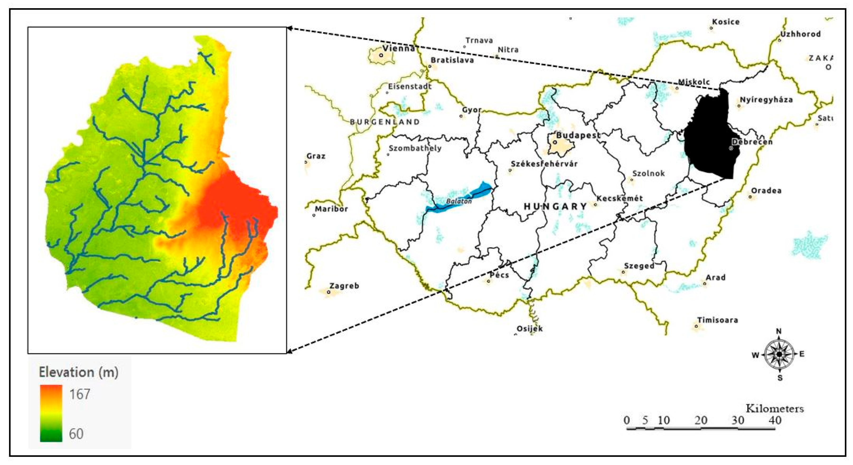
2.1. Study Area

A proportion of TIKEVIR in eastern Hungary was considered as a test site in this study (Figure 1). This region is characterized by a temperate climate and is a vital hydrological and agricultural area, located in the Great Hungarian Plain along the rivers Tisza and Körös, respectively. The region is crucial for irrigated industrial crop production such as corn, winter and spring wheat, sunflower, and pastures, which play a big role in Hungary’s food security and economy [37]. The region’s hydrological significance routes from its extensive irrigation, river, and flood control networks, playing a vital role in groundwater recharge, wetland ecosystems, and drought risk mitigation [38]. However, climate change and human activity impacts in this region are affecting water availability, making it necessary to monitor land cover to enhance irrigation efficiency, detect changes in wetland areas, and ensure sustainable water resources utilization [39].

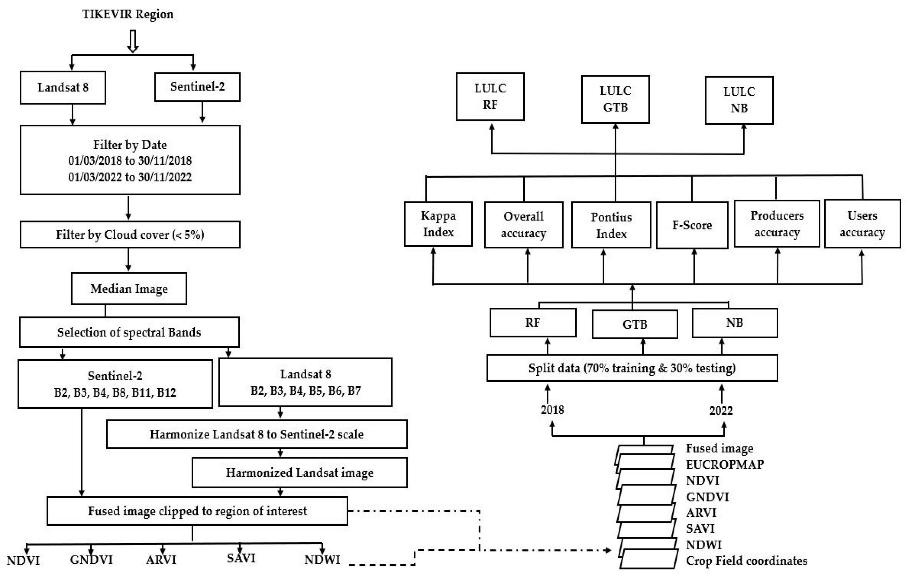
2.2. Workflow Description

The study started with the acquisition of satellite imagery for 2018 and 2022, respectively (Figure 2), from Landsat 8 operational land imager (OLI) and Sentinel-2 multispectral instrument (MSI), whose spectral data are outlined in

Table 1. Satellite sensor spectral Input data.

Sensor	Band	Color Description	Wavelength (µm)	Resolution (m)
Landsat 8	B2	Blue	0.482	30
	B3	Green	0.561	30
	B4	Red	0.655	30
	B5	Near-Infrared (NIR)	0.865	30
	B6	Shortwave infrared 1 (SWIR—1)	1.609	30
	B7	Shortwave infrared 2 (SWIR—2)	2.201	30
Sentinel-2	B2	Blue	0.49	10
	B3	Green	0.56	10
	B4	Red	0.665	10
	B8	Near-Infrared (NIR)	0.842	10
	B11	Shortwave infrared 1 (SWIR—1)	1.61	20
	B12	Shortwave infrared 2 (SWIR—2)	2.19	20

. Landsat 8 imagery was sourced from the Collection 2 Tier 1 Top-of-Atmosphere Reflectance dataset (LANDSAT/LC08/C02/T1_TOA), which offers top-of-atmosphere (TOA) reflectance without atmospheric adjustment [40,41]. Sentinel-2 imagery, on the other hand, came from the Level-2A Surface Reflectance dataset (COPERNICUS/S2_SR), which was atmospherically corrected by the European Space Agency (ESA) using the Sen2Cor algorithm before being fed into Google Earth Engine [42,43]. The reference training and validation data were collected from the Hungarian crop area inventory of the TIKEVIR and EUCROPMAP from the Joint Research Centre [44,45].

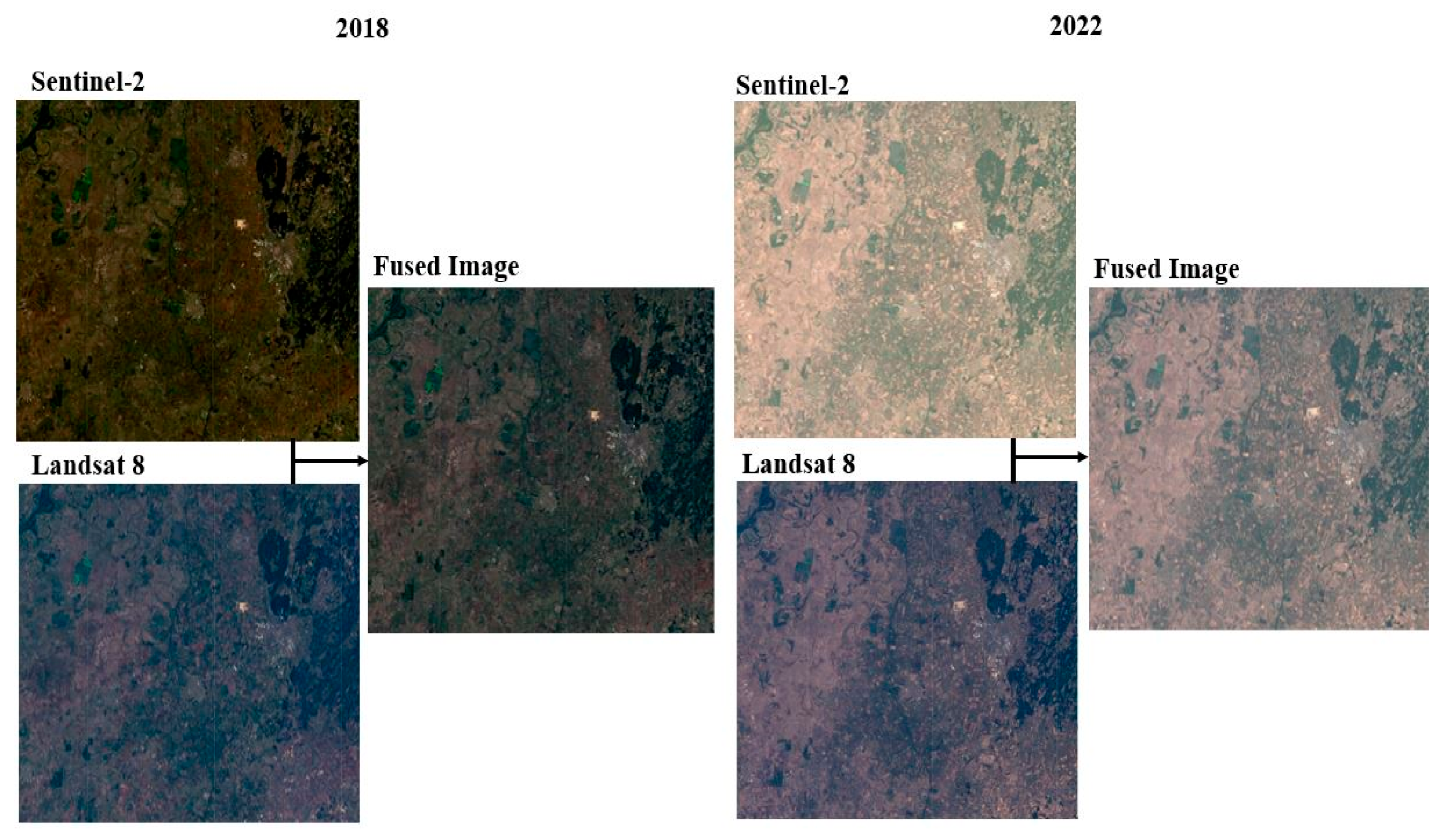
2.2.1. Harmonization of Landsat 8 Imagery to the Sentinel-2 Scale

Landsat 8 and Sentinel-2 median images across the two cropping periods of 2018 and 2022 were obtained with properties outlined in Table 1. Due to the differences in sensor properties, radiometric calibration, and spectral response functions, ensuring consistency in our final fused composite imagery necessitated the harmonization of these two optical satellite families into one scale. The process involved combining Landsat 8 and Sentinel-2 images by averaging the reflectance values of each respective sensor band to leverage the strengths of both datasets (Figure 3).

Sentinel-2 has a higher spatial resolution of 10 m for visible, near infrared bands and 20 to 60 m for Shortwave Infrared bands with frequent revisit times of 5 to 10 days, compared to Landsat 8, which provides most of the spatial resolution at 30 m with longer revisit cycles of 16 days. Fused median composite images of Sentinel-2 and Landsat 8 were created for the peak vegetation period in both 2018 and 2022 with an overall aim of overcoming data gaps and enhancing spectral richness. While Sentinel-2 offers high spatial resolution, its imagery was occasionally incomplete during key phenological windows. The integration of Landsat 8 helped fill these spatial gaps and introduced additional spectral bands, particularly in the shortwave infrared region, to support improved vegetation differentiation. The fused median image provided a more spatially consistent and spectrally diverse base for deriving vegetation indices and conducting classification. This enhanced the separability of spectrally similar classes, such as cropland and grassland, and supported a more balanced and reliable training input across the landscape. Although only a single composite was used per year, this fusion helped mitigate data quality issues and improved the robustness of the classification process. The harmonization process was in accordance with Claverie et al. [46], Roy et al. [47], and

Table 2. Scale factors for harmonizing the Landsat 8 operational land imager (OLI) to the Sentinel-2 multispectral instrument (MSI) scale.

Band	Conversion	Scale Factor (Fx)
Blue	OLI(B2)—MSI (B2)	1.05
Green	OLI(B3)—MSI (B3)	1.03
Red	OLI(B4)—MSI (B4)	1
NIR	OLI(B5)—MSI (B8)	0.98
SWIR I	OLI(B6)—MSI (B11)	0.97
SWIR 2	OLI(B7)—MSI (B12)	0.96

.

H_xL8 = F_xL8_r

(1)

FI = 0.5(H_xL8 + S2_r)

(2)

where H_xL8 is the harmonized reflectance for Landsat 8 band, F_x denotes a band-specific scale factor, L8_r is the Landsat 8 reflectance adjusted to Sentinel-2 scale, FI is the fused image, and S2_r is the Sentinel-2 reflectance.

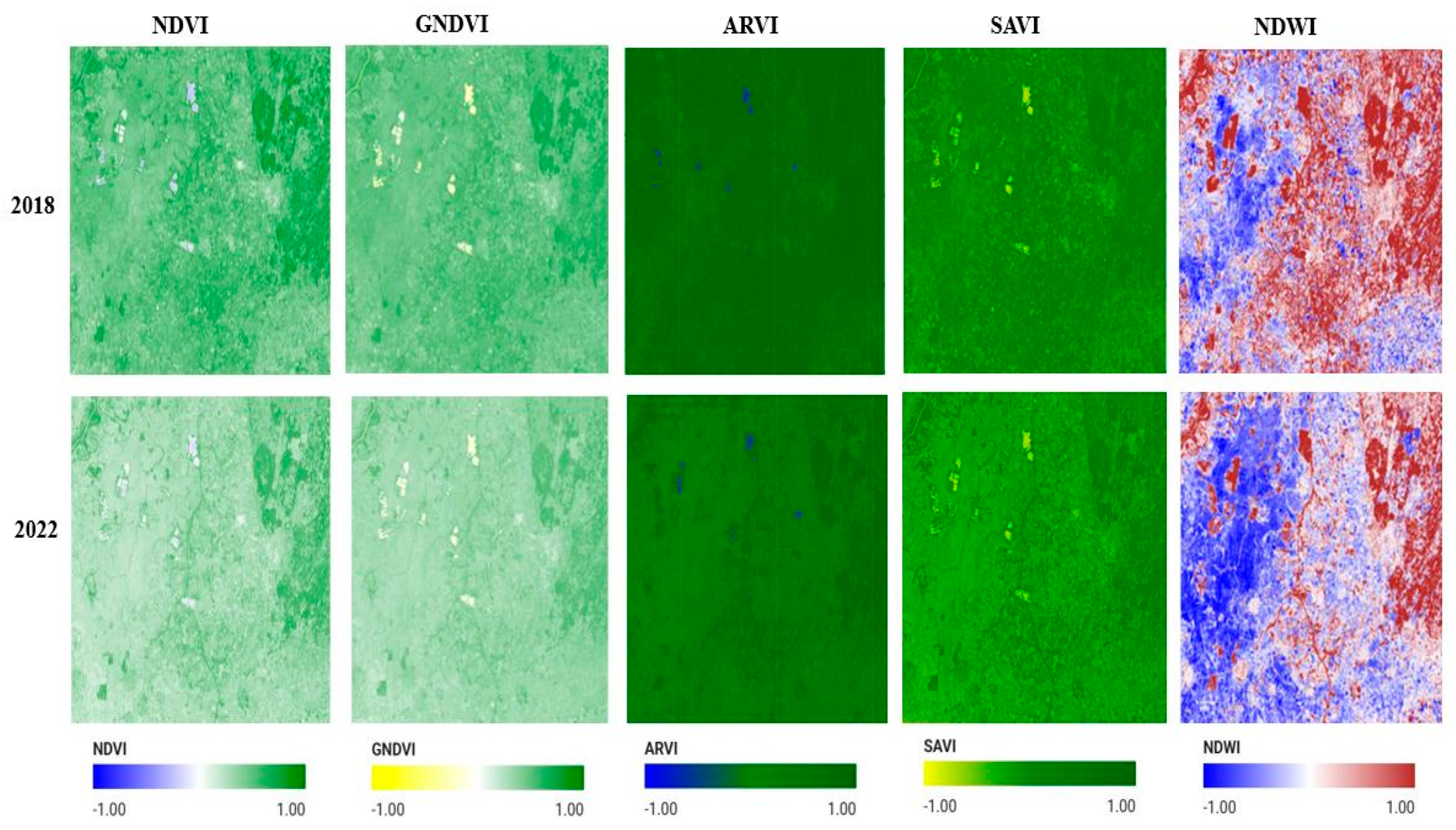
2.2.2. Spectral Indexing

Five spectral indices, namely Normalized Difference Vegetation Index [48], Green Normalized Difference Vegetation Index [49], Atmospherically Resistant Vegetation Index [50], Soil-Adjusted Vegetation Index [51], and Normalized Difference Water Index [52], were used to enhance land cover classification accuracy (

Table 3. Spectral index input data description.

Index	Description	Formulae Used	References
NDVI	Normalized Difference Vegetation Index	(NIR − Red)/(NIR + Red)	Rouse et al. [48]
GNDVI	Green Normalized Difference Vegetation Index	(NIR − Green)/(NIR + Green)	Gitelson et al. [45]
ARVI	Atmospheric Resistant Vegetation Index	(NIR − (Red − (1 ∗ (Blue − Red))))/(NIR + (Red − (1 ∗ (Blue − Red))))	Kaufman and Tanre [50]
SAVI	Soil-Adjusted Vegetation Index	((NIR − Red) ∗ (1 + 0.5)/(NIR + Red + 0.5)	Huete [51]
NDWI	Normalized Difference Water Index	(NIR − SWIR1)/(NIR + SWIR1)	Mcfeeters [52]

).

NDVI was used to differentiate the vegetation from non-vegetated areas by measuring the density and health of vegetation. GNDVI was employed to improve sensitivity to chlorophyll content and detect variations in crop health, whereas ARVI reduced atmospheric effects in vegetation and solved the effects of aerosol hindrance in the vegetation analysis. SAVI minimized the soil background influence in sparsely vegetated regions of the test site [51]. Additionally, in thick vegetation areas, it has been demonstrated that a negative soil adjustment factor in SAVI improves LAI estimation and lessens saturation effects [53]. NDWI was used to identify water bodies (Table 3). These indices were computed from the fused composite image of the respective cropping periods of 2018 and 2022 and integrated as additional classification features in Google Earth Engine (Figure 2 and Figure 4).

Despite the mathematical similarities and established correlation between NDVI and SAVI, they were both included because of their different levels of sensitivity to vegetation conditions. Although this addition enhances the characterization of the vegetation, it might add multicollinearity to the feature collection. This restriction was acknowledged in this study to maintain each index’s complementary strengths.

2.2.3. Integration of Spectral Indices, Reference Data, and Machine Learning Classifiers

Machine learning-based land cover classification was implemented using RF, GTB, and NB classifiers in Google Earth Engine. These three classifiers were chosen because of their unique attributes For example, RF is an ensemble learning classifier that can build multiple decision trees using feature randomization to reduce overfitting of training data in highly dimensional data while enhancing accuracy [54]. GTB also constructs trees in a logical and uniform manner while minimizing errors through gradient descent, resulting in high accuracy [17]. NB bases Bayes’ theorem for probabilistic classification, making it computationally efficient and well-suited for land cover classification [20]. Multiple datasets were integrated as part of a supervised strategy to increase classification accuracy and feature representation. These comprised ground-truth field position points for training and validating the models from the Hungarian agricultural reference inventory as the primary reference data to achieve a secondary reference dataset, consisting of EUCROPMAP, which was used for crop types and land cover distribution. Five spectral indices, namely NDVI, GNDVI, ARVI, SAVI, and NDWI, were calculated from the combined Landsat 8 and Sentinel-2 data and merged into a single image stack with the reference data using Google Earth Engine’s add Bands function from which the classifier could access all input data at once during training, while maintaining the spectral and spatial information of each layer (Figure 2). Although the Hungarian agricultural reference inventory provided extensive regional coverage, reference bias could have been introduced since it excluded vegetation in informal and urban settings. Also, field data were gathered during vegetation peaks, and spectral inconsistencies may have been induced by phenological variability and regional heterogeneity, particularly during the drought period experienced in 2022. The primary source of ground truth data for classifier training and validation was the Hungarian Crop Reference Inventory, which offers plot-level, field-verified land cover designations for the entire TIKEVIR region. This was enhanced by using the EUCROPMAP dataset as a secondary reference source to ensure geographic consistency and class representation, particularly in cases where field data were scarce. Crucially, EUCROPMAP was not utilized to evaluate or infer land dynamics; instead, the categorization results were based on machine learning outputs from fused Sentinel-2 and Landsat 8 data, which were verified against the official Hungarian inventory.

RF, GTB, and NB classifiers were implemented using Google Earth Engine’s grin library under supervision, trained and tested using a total of 800 ground-truth points from the Hungarian agricultural reference inventory. These comprised 100 samples for each of the eight land cover classes: water bodies, built-up areas, mixed forests, corn, sunflower, winter wheat, grassland, and other crop types. The training was performed on 70% of each dataset (n = 560) and 30% (n = 240) was used in evaluating accuracy metrics (Figure 2) such as Kappa coefficient, Overall Accuracy, Pontius index, precision, and recall in determining performance of the classification process (

Table 4. Accuracy metrics used in validating the classification algorithms’ performance.

Abbreviation	Accuracy Metric	Formulae Used	References
PA	Producers’ Accuracy/Recall	= ${\displaystyle \frac{P}{P + FN}}$	Congalton [55]	(3)
UA	Users’ Accuracy/Precision	= ${\displaystyle \frac{P}{P + FP}}$	Congalton [55]	(4)
F1 score	F1 score	= 2 · ${\displaystyle \frac{\mathrm{UA} \times \mathrm{PA}}{\mathrm{UA} + \mathrm{PA}}}$	Van Rijsbergen [56]	(5)
OA	Overall Accuracy	= ${\displaystyle \frac{\sum P+ TN}{\sum (P+FP+FN+TN)}}$	Foody [57]	(6)
KC	Kappa Coefficient	= ${\displaystyle \frac{(Y-Z)}{(1-Z)}}$	Cohen [58]	(7)
PI	Pontius Index	= 1 − ${\displaystyle \frac{\sum _i\left|A_{i-P_i }\right|}{2·GT}}$	Pontius and Schneider [59]	(8)

Where P is for the correctly classified pixels of a given land cover class (True positive), FN for the missed pixels of a given land cover class (False Negative), FP for the incorrectly classified pixels of a given land cover class (False positives), TN for the correctly rejected pixels (True Negatives), Y for the proportion of pixels that were correctly classified (observed accuracy), Z for the expected proportion of correct pixels based on random chance (Expected accuracy), A_i for the total occurrences for each class in the confusion matrix; P_i for the total predicted occurrences for each class in the confusion matrix, and GT for the grand total of all classes in the confusion matrix.

). The 70/30 train-test subsets were divided using Google Earth Engine’s random column method, which gives each sample a pseudo-random value for randomized and repeatable splitting. The division was not stratified nor spatially clustered because this procedure was conducted consistently across all land cover classifications. To guarantee consistency in performance evaluation, the same subset division was used for training and testing all classifiers (RF, GTB, and NB), enabling a reproducible and objective partitioning. The RF model was set up with 100 trees and all internal parameters left at their default settings due to Google Earth Engine’s limited parameter control. In total, 100 trees, a sampling rate of 0.7, and a learning rate of 0.1 were employed in the GTB classifier. The NB classifier used Google Earth Engine’s default configuration, which does not expose variable hyperparameters.

2.2.4. Overall and Interclass Accuracy Evaluation

The Overall Accuracy (6) was employed to measure the percentage of correctly classified pixels relative to the total validated samples by providing a general indication of each model’s performance. The Kappa Coefficient (7) was used to account for the random consistency possibility between predicted and actual land cover classes, whereas the Pontius Index (8) was used to evaluate the allocation and quantity inconsistency in analyzing the spatial accuracy of land cover predictions while identifying systematic errors. Precision (4) was employed to measure the proportion of correctly classified samples for each land cover class in assessing the reliability of the predictions for each land cover class. Recall (3) was used to evaluate the classifiers’ ability in correctly identifying the total pixels belonging to a given land cover class, and lastly, the F1 score (5) was employed to provide balance between precision and recall in circumstances where land cover class distribution was uneven (Table 4).

Despite the Kappa Coefficient being widely used for evaluating inter-rater agreement, it is noted to have certain limitations, especially imbalanced classes as well as marginally distributed classes, which often leads to underestimation in the agreements of the classification datasets [59,60]. For this reason, alternative metrics such as the Pontius Index, F1 score, User’s Accuracy (UA), Producer’s Accuracy (PA), and Overall Accuracy are used in this study to better handle the imbalances in the data as well as provide insights into the specific land cover classes [59,61].

2.3. Post Classification Analysis

The detection and quantification of land cover changes between 2018 and 2022 were performed using outputs of the best classifier. Metrics such as percentage land cover changes were computed to provide insights into the dynamics of land cover transformation between the two reference periods of 2018 and 2022, respectively.

3. Results

3.1. Dominant Land Use Categories in the Test Site

The dominant categories of land use in the test site covering an area of 4111.6 km² of the TIKEVIR were mapped out using three different machine learning algorithms, namely, Random Forest (Figure 5a), Gradient Tree Boosting (Figure 5b), and Naive Bayes (Figure 5c). These land cover classes included water bodies, built-up areas, mixed forests, corn, sunflower, winter wheat, grassland, and other crop types during the cropping periods of 2018 and 2022. There was a notable similarity and variation in land cover class predictions by RF, GTB, and NB classifiers in both reference cropping periods of 2018 and 2022, respectively. Across both years, grasslands consistently had the highest classified area, although RF and GTB produced higher grassland areas than NB (Figure 5a–c). Water bodies maintained a relatively stable coverage across all classifiers, with minimal variations, except in 2022 for GTB, which showed an increment due to misclassification (Figure 5b). Notable variations in winter wheat and other crops classification were observed, with NB predicting higher acreage in 2022, while RF and GTB showed a balanced trend in the respective land cover classes (Figure 5a–c).

Corn and winter wheat remained among the dominant classified crops in the test site throughout the three classifiers, although RF in 2022 recorded the highest increment in corn coverage (Figure 5a). Sunflower classifications showed the highest discrepancy, with NB in 2018 predicting higher acreages compared to RF and GTB but aligning more closely in 2022 (Figure 5a–c). The other crop land cover category exhibited a considerable variation across the classifiers, with Naive Bayes exhibiting higher acreages, particularly in 2022 (Figure 5c). Overall, RF and GTB produced more stable classifications across the cropping periods of 2018 and 2022, respectively, while NB displayed greater fluctuations (Figure 5a–c).

Narrowing down our analysis by masking out the Debrecen area from the broader TIKEVIR region, it can be noted that RF and GTB were consistent with the satellite images for 2018 and 2022, respectively (Figure 6). This further demonstrates the effectiveness of RF and GTB in producing land cover maps for supporting satellite yield estimates as well as budgeting water resources for irrigated fields.

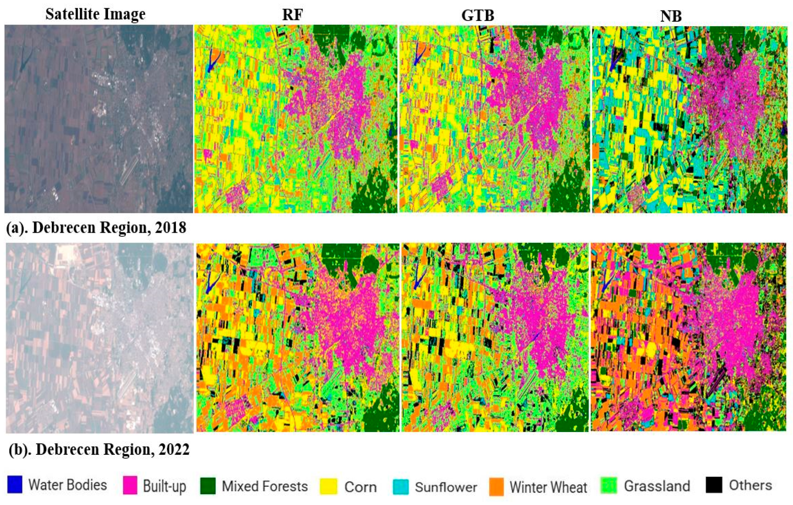
3.2. Land Cover Classification Performance Comparison

RF, GTB, and NB showed key variations in the classification performance (

Table 5. General accuracy assessment in land cover classification. RF denotes Random Forest, GTB refers to Gradient Tree Boosting, NB to Naive Bayes, while OA, KC, and PI represent Overall Accuracy, Kappa Coefficient, and Pontius Index, respectively.

	2018			2022
	OA	KC	PI	OA	KC	PI
RF	0.87	0.83	0.94	0.82	0.78	0.86
GTB	0.81	0.76	0.97	0.84	0.8	0.90
NB	0.61	0.52	0.82	0.75	0.69	0.95

). In 2018, RF achieved the highest Overall Accuracy (OA) of 0.87 and Kappa Coefficient (KC) of 0.83 (Table 5), indicating strong agreement with TIKEVIR reference data from the Hungarian crop reference inventory, while GTB followed with an OA of 0.81 and a KC of 0.76 (Table 5). However, GTB recorded the highest Pontius Index (PI) of 0.97, suggesting better spatial allocation accuracy. NB had the least performance, with an OA of 0.61 and KC of 0.52, indicating weaker land cover classification reliability (Table 5). In 2022, RF declined to an OA of 0.82, a KC of 0.78, and a PI of 0.86 compared to those of 2018 (Table 5), while GTB improved to an OA of 0.84, a KC of 0.80, and a PI of 0.90 (Table 5), demonstrating more classification stability. NB improved its Overall Accuracy to 0.75 but produced the least KC of 0.69, due to struggles in maintaining agreement with training data labels despite an increase in the PI of 0.95 (Table 5). These results demonstrate the least reliability of NB compared to ensemble-based models like RF in land cover classification (Table 5).

Based on the comparisons of other accuracy performance metrics for class-specific categorization, Producer’s Accuracy (PA), User’s Accuracy (UA), and F1 Score are assessed across the land cover classes (

Table 6. Land cover class-wise performance comparison. RF denotes Random Forest, GTB refers to Gradient Tree Boosting, NB to Naive Bayes, while PA and UA represent Producers’ Accuracy and Users’ Accuracy, respectively.

		2018			2022
	Class	PA	UA	F1 Score	PA	UA	F1 Score
RF	Water bodies	1	1	1	1	1	1
	Built- up	0.72	0.87	0.79	0.69	1	0.82
	Mixed Forests	1	0.89	0.94	1	1	1
	Corn	0.8	0.89	0.76	1	0.71	0.83
	Sunflower	0.67	0.67	0.8	0	0	0
	Winter wheat	1	1	1	0.75	0.75	0.75
	Grassland	1	0.88	0.94	0.93	0.7	0.8
	Others	1	1	1	0.5	1	0.67
GTB	Water bodies	1	1	1	1	0.83	0.91
	Built- up	0.72	0.76	0.74	0.85	1	0.92
	Mixed Forests	1	1	1	1	1	1
	Corn	0.8	0.89	0.84	1	0.71	0.83
	Sunflower	0.5	0.38	0.43	0	0	0
	Autumn wheat	0.5	1	0.67	0.5	1	0.67
	Grassland	0.91	0.91	0.91	0.87	0.76	0.81
	Others	1	0.5	0.67	0.67	0.8	0.73
NB	Water bodies	1	1	1	1	1	1
	Built- up	0.61	0.79	0.69	0.77	0.83	0.8
	Mixed Forests	0.88	0.78	0.83	0.67	0.33	0.44
	Corn	0.7	0.88	0.78	0.4	0.67	0.5
	Sunflower	0.33	0.13	0.19	0	0	0
	Winter wheat	0.5	1	0.67	0.75	0.75	0.75
	Grassland	0.57	0.81	0.67	0.73	0.73	0.73
	Others	0	0	0	0.83	0.83	0.83

). RF and GTB consistently outperformed NB, particularly in land cover classes of corn, winter wheat, and mixed forests (Table 6). In 2022, RF maintained high accuracy for water bodies and mixed forests with a PA of 1, UA of 1, and F1 score of 1, respectively (Table 6), while NB significantly misclassified mixed forests, yielding a PA of 0.67, UA of 0.33, and F1 score of 0.44, respectively (Table 6). GTB performed slightly better than RF for built-up areas with an F1 score value of 0.92 compared to 0.82 for RF (Table 6), indicating strength in classifying urban areas. Sunflower was totally misclassified, yielding a PA, UA, and F1 value of 0, respectively, across all classifiers in 2022, highlighting a challenge in distinguishing this crop compared to other vegetation categories (Table 6).

3.3. Land Cover Dynamics in the Test Site Between the Two Cropping Reference Periods of 2018 and 2022

Using RF output as the best land cover classifier, the land cover changes in the TIKEVIR region between 2018 and 2022 show significant shifts across the land cover categories (

Table 7. Comparisons of the land cover classification results of the land use categories in the TIKEVIR region by the three machine learning classifiers.

		2018			2022
		RF	GTB	NB	RF	GTB	NB
Area (Sq. Km)	Water Bodies	57.0	59.1	52.7	57.8	109.0	52.8
	Built-up	397.2	533.1	282.3	433.7	375.3	626.4
	Mixed Forests	226.0	210.9	272.3	193.4	131.1	348.8
	Corn	774.4	807.1	607.7	996.5	660.8	656.6
	Sunflower	164.0	234.7	873.3	83.8	70.8	206.1
	Winter Wheat	335.8	317.5	270.8	510.5	427.8	653.2
	Grassland	2150.2	1928.8	1357.4	1693.8	2128.3	941.8
	Others	7.2	20.5	395.1	142.1	208.6	625.9
	Total (4111.6)
% cover	Water Bodies	1.4	1.4	1.3	1.4	2.7	1.3
	Built-up	9.7	13.0	6.9	10.5	9.1	15.2
	Mixed Forests	5.5	5.1	6.6	4.7	3.2	8.5
	Corn	18.8	19.6	14.8	24.2	16.1	16.0
	Sunflower	4	5.7	21.2	2.0	1.7	5.0
	Winter Wheat	8.2	7.7	6.6	12.4	10.4	15.9
	Grassland	52.3	46.9	33.0	41.2	51.8	22.9
	Others	0.2	0.5	9.6	3.5	5.1	15.2

). A minor increase from 57.0 km² in 2018 to 57.8 km² in 2022 (1.4%) of water bodies; built-up areas expanded from 9.7% to 10.5%; mixed forests declined from 5.5% to 4.7%. Corn cultivation increased significantly from 18.8% to 24.2%, while sunflower cultivation decreased from 4.0% to 2.0%. The winter wheat area also increased from 8.2% to 12.4% (Table 7), whereas grassland showed a decline from 52.3% to 41.2% and the other land cover category grew from 0.2% to 3.5% (Table 7).

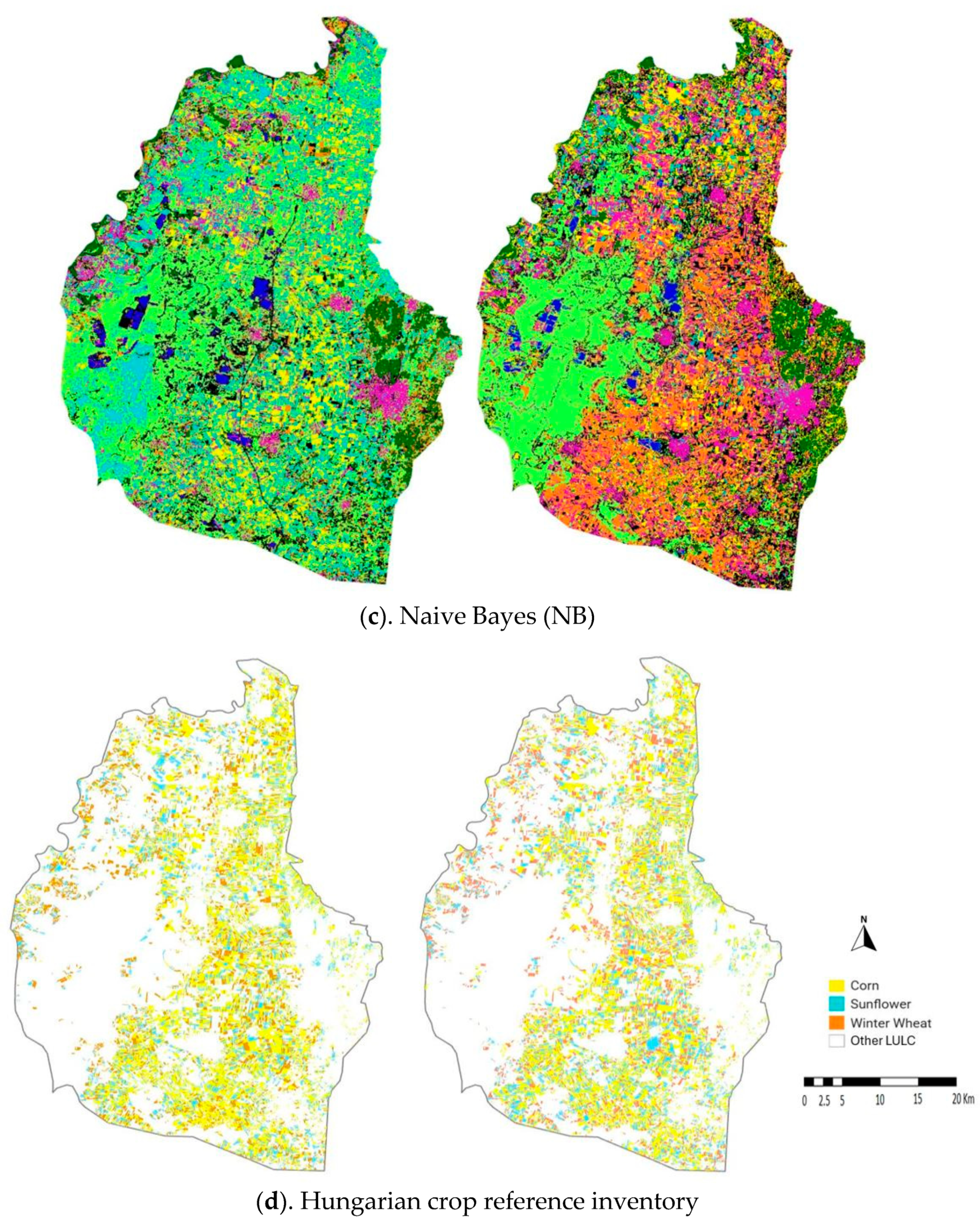
3.4. Comparison of the Machine Learning Classification Results with the TIKEVIR Reference Data

Further validation and best classifier evaluation were conducted by comparing the results of RF, GTB, and NB for 2018 and 2022 against the primary reference land use data from the Hungarian crop reference inventory for the TIKEVIR region and secondary reference from the EUCROPMAP, respectively (

Table 8. Primary and secondary reference data used in the sample area within the TIKEVIR for land cover accuracy validation. HU-CRI denotes the Hungarian crop reference inventory, and EU-Crop refers to EUCROPMAP.

S/No.	Land Use Class	Area (Sq. Km)				% Cover
		2018		2022		2018		2022
		HU-CRI	EU-Crop	HU-CRI	EU-Crop	HU-CRI	EU-Crop	HU-CRI	EU-Crop
1	Water Bodies	-	-	-	-	-	-	-	-
2	Built-up	-	-	-	-	-	-	-	-
3	Mixed Forests	16.53	-	29.5	-	0.4	-	0.7	-
4	Corn	866.81	1053	894.9	1144.1	22.1	27.1	22.8	28.8
5	Sunflower	458	314.4	538.7	333	11.7	8.1	13.7	8.4
6	Winter Wheat	472	431.5	483.6	598.8	12	11.1	12.3	15.1
7	Grassland	1142.11	1244.2	1155.3	1105.3	29.1	32.0	29.4	27.8
8	Others	972.5	843.4	829.2	792	24.8	21.7	21.1	19.9
	Total Cropped Area	3928	3886.5	3931.1	3973.2	100	100	100	100

). The most consistent land cover category was corn, where RF estimated 774.4 km² in 2018 and 996.5 km² in 2022, closely aligning with the TIKEVIR primary reference values of 866.81 km² in 2018 and 894.9 km² in 2022 (Table 7 and Table 8). Mixed forests, however, showed variations across all three classifiers, with RF estimating 226.0 km² in 2018 and 193.4 km² in 2022, much higher than the primary reference values of 16.53 km² in 2018 and 29.5 km² in 2022. Grasslands were overestimated by the three classifiers, especially RF, which predicted 2150.2 km² in 2018 and 1693.8 km² in 2022 (Table 7 and Figure 6), while the primary reference values were 1142.11 km² and 1155.3 km², respectively (Table 8).

Among the three classifiers tested, RF demonstrated the highest consistency with the primary reference dataset across multiple land cover classes, particularly in corn and winter wheat (Table 7 and Table 8). A stable estimation was maintained by RF for winter wheat, predicting 335.8 km² in 2018 and 510.5 km² in 2022, compared to the primary reference values of 472 km² in 2018 and 483.6 km² in 2022 (Table 7 and Table 8). GTB showed improved estimates for mixed forests in 2022 but underestimated corn and grasslands, while NB had the most non-coherent variations across the land cover classes, particularly in 2018.

4. Discussions

4.1. The Efficiency of Machine Learning Classifiers in Mapping Land Cover

The comparison of Random Forest (RF), Gradient Tree Boosting (GTB), and Naive Bayes (NB) classifiers reveals that ensemble learning methods, particularly RF and GTB, are more effective in generating accurate land cover maps in heterogeneous agricultural regions like TIKEVIR. Throughout the two cropping years (2018 and 2022), RF performed the best, achieving excellent classification accuracy and alignment with reference datasets. This confirms the results of earlier research that supported the resilience and dependability of RF in mapping land cover and classifying crops because of its capacity to manage intricate, non-linear interactions in remote sensing data. Similar studies have reported RF accuracies to fall between 0.80 to 0.90 for crop classification according to Belgiu and Drăguţ [15] and Maxwell et al. [28], thus supporting the robustness of the RF classifier in heterogeneous landscapes. The limits of NB in handling multi-dimensional feature spaces, which are prevalent in satellite data, were demonstrated by its reduced dependability and increased susceptibility to misclassification. Potential multicollinearity may have been introduced into the feature space due to the similarity in how some spectral indices, such as NDVI and SAVI, are derived using the same spectral bands. Classifiers that depend on the assumption of conditional independence among input variables, such as NB, are especially vulnerable to this issue. There could have been a possibility that the model’s efficacy was diminished by the presence of strongly correlated indices, which also caused overfitting and skewed generalization for minority classes, such as the other crop category. This makes NB unsuitable for precise land cover discrimination in complex environments, as evidenced by its uneven and generally poor performance in both classification and agreement metrics. Such patterns are consistent with other research showing ensemble approaches perform better than more straightforward probabilistic classifiers in distant sensing tasks [16,21].

4.2. Class-Specific Classification Challenges

Classifier performance varied significantly across land cover classes. RF and GTB were highly accurate for water bodies, mixed forests, and major crops like corn and winter wheat. The complete misclassification of sunflowers in 2022 is attributed to the severe drought that year, which altered vegetation patterns and spectral signatures; coupled with possible phenological shifts, it could have likely led to confusion of the classifiers with other classes, hence reducing model accuracy. From the results shown in Table 6, RF emerged as the most reliable classifier overall compared to GTB and NB, offering the best balance between accuracy, class differentiation, and spatial consistency, although GTB showed improvements in 2022, particularly for built-up areas. NB, while improving in 2022, remains inconsistent and is not recommended for high-accuracy land cover classification. Another factor contributing to the misclassification is the influence of a few training samples for underrepresented crops, which is a problem identified in numerous remote sensing research [62]. These results demonstrate the necessity of using balanced training datasets and taking environmental variability into account when creating models.

4.3. Limitations of the Model and Class Imbalance

Although classifier results differed, grasslands dominated the area in both reference years. Compared to NB, which frequently overestimated grassland acreage, RF and GTB consistently recorded larger areas. Corn and winter wheat were the most prevalent agricultural land cover, demonstrating their dominance in the cropping system. As a result of the model’s difficulties with spectral ambiguity, NB tended to overestimate several classes, such as sunflower and mixed forests, especially when phenological changes occurred. The substantial difference in grasslands and mixed forested areas between the machine learning classification outputs and the primary reference data arises because the Hungarian authority does not account for urban greening infrastructure or vegetation, such as trees and grasses, in the settlement areas and along roadsides. Their data includes only commercially cultivated trees and grasses on plot scales. In contrast, the classification considers all vegetation types across the entire TIKEVIR region.

Classifier sensitivity to less frequent land use classifications may have been impacted by the 70/30 train-test split, even though it was statistically acceptable. According to He and Garcia [63], class imbalance can lower model accuracy for uncommon categories, which is a known problem in many classification workflows. The random, non-variable 70/30 split technique used in the construction of training and testing datasets made randomized splitting easier by giving each reference sample a consistently distributed random value. However, both the training and testing subsets could have maintained the original dataset’s class distribution, which included the predominance of grassland, and the low prevalence of minority classes like other land use categories. The classifier’s performance could have been impacted by this uneven class distribution.

4.4. Dynamics of Land Use Change and Intensification of Agriculture

The observed land cover changes over the two reference periods (2018–2022) reveal notable agricultural intensification and urban expansion, both of which have significant implications for water resources. A move toward more water-dependent crops is indicated by the rise in the production of corn and winter wheat (Table 7), which could put more strain on nearby water supplies by raising the need for irrigation. At the same time, the loss of natural vegetation like grasslands and mixed forests (Table 7) diminishes the landscape’s ability to regulate runoff, recharge groundwater, and allow for natural water infiltration. This could result in increased surface water variability and increased risk of flooding. The expansion of built-up areas exacerbates these issues by increasing impervious surfaces, which can further reduce infiltration, accelerate stormwater runoff, and degrade water quality. According to Foley et al. [64], these developments are consistent with global trends where urbanization and intensification alter hydrological systems, frequently resulting in water scarcity or degradation if not well managed. For agricultural productivity and water sustainability to coexist, these changes necessitate integrated land and water management approaches. Prior studies have underscored the need to integrate hydrological models with land cover data to facilitate irrigation planning and drought alleviation [65]. The findings of this study support this need, especially in view of the changing climate and growing human strain.

5. Conclusions

This study evaluated the performance of three machine learning classifiers, namely Random Forest, Gradient Tree Boosting, and Naive Bayes, for land cover classification using a portion of the Tisza-Körös Valley Irrigation System region (TIKEVIR) in Hungary. Two reference cropping periods, wet and dry seasons from 2018 and 2022, respectively, were used to test the classifiers’ capabilities in land cover mapping. The results were compared with each other and validated against primary reference data from the Hungarian crop reference inventory for the TIKEVIR region. RF outperformed GTB and NB in terms of Overall Accuracy, Kappa Coefficient, and consistency with primary and secondary reference land use data. RF also exhibited the highest reliability in major agricultural classes, including corn and winter wheat, aligning closely with primary reference values of the Hungarian crop reference inventory for the TIKEVIR region. Although GTB was effective in classifying mixed forests, it tended to underestimate crop areas, while NB displayed the greatest inconsistencies, particularly in grassland and sunflower classifications.

This research indicates that Random Forest has demonstrated exceptional classification capabilities in the TIKEVIR region, hence bolstering its application in complex agricultural environments. While the findings are region-specific, they underscore the critical importance of robust land cover classification in hydrological monitoring and sustainable water resource planning. Future studies should concentrate on integrating these classifications with dynamic hydrological models so that adaptive irrigation techniques and real-time monitoring are possible. Although the focus of this study was on land cover classification, the implications extend directly to irrigation planning, crop monitoring, and adaptive resource allocation under increasing climatic variability. The TIKEVIR region, being central to Hungary’s irrigated agriculture, benefits from such accurate mapping tools to inform practical decisions on water use management and land-use sustainability. This study tackles recurring land cover classification issues in Hungary’s TIKEVIR system, an agriculturally and ecologically vital floodplain, therefore advancing regional-scale remote sensing applications. In line with EU agri-environmental goals, our findings may help guide sustainable irrigation management plans and provide useful insights for vegetation monitoring in a range of hydrological situations.

Overall, the fusion of optical imagery with spectral indices enhanced land cover classification, whose integration with machine learning classifiers can be beneficial in supplementing empirical hydrological models to provide a comprehensive framework for decision support for sustainable management of water resources, appropriation, and ensuring efficient agricultural practices. Although the spatial resolution and composite approach of both Sentinel-2 and Landsat 8 datasets were harmonized, we recognize that disparate correction levels could generate slight discrepancies in reflectance. Future research could investigate more harmonization through surface reflectance calibration to enhance uniformity. Similarly, having strongly correlated indices can make the model less successful and cause overfitting and biased generalization, particularly when minority groups have less training data. We acknowledge that formal sensitivity and feature importance analyses are necessary for future research, even though they were not included in this study. Correlation-based feature selection and dimensionality reduction techniques such as Principal Component Analysis (PCA) may be used to lessen input dataset redundancy and increase model resilience.

According to our findings, phenological stage and interannual climate variability, such as the drought circumstances in 2022, may have a significant impact on class separability, especially for crop types like sunflower. To enhance classification accuracy and better capture crop-specific spectral trajectories, future research should integrate multi-temporal imaging throughout the growth season. The integration of categorized outputs with hydrological modeling frameworks, combining RF with deep learning techniques, may be further investigated in future studies to improve the precision and adaptability to dynamic land cover changes.

References

1. IPCC. Climate Change and Land: An IPCC Special Report on Climate Change, Desertification, Land Degradation, Sustainable Land Management, Food Security, and Greenhouse Gas Fluxes in Terrestrial Ecosystems; Shukla, P.R., Skea, J., Calvo Buendia, E., Masson-Delmotte, V., Zhai, P., Pörtner, H.-O., Roberts, D., Slade, R., Connors, S., van Diemen, R., et al., Eds.; Intergovernmental Panel on Climate Change: Geneva, Switzerland, 2019; Report released on 8 August 2019; Available online: https://www.ipcc.ch/site/assets/uploads/sites/4/2022/11/SRCCL_Full_Report.pdf (accessed on 1 January 2025).
2. FAO. The State of the World’s Land and Water Resources for Food and Agriculture—Systems at Breaking Point (SOLAW 2021); FAO eBooks: Rome, Italy, 2021; Report released on 9 December 2021. [Google Scholar] [CrossRef]
3. Van Daalen, K.R.; Tonne, C.; Semenza, J.C.; Rocklöv, J.; Markandya, A.; Dasandi, N.; Jankin, S.; Achebak, H.; Ballester, J.; Bechara, H.; et al. The 2024 Europe report of the Lancet Countdown on health and climate change: Unprecedented warming demands unprecedented action. Lancet Public Health 2024, 9, e495–e522. [Google Scholar] [CrossRef]
4. Lovejoy, T.E.; Nobre, C. Amazon Tipping Point. Sci. Adv. 2018, 4, eaat2340. [Google Scholar] [CrossRef] [PubMed]
5. Shah, T. Groundwater Governance and Irrigated Agriculture; (No. 19); Global Water Partnership (GWP): Stockholm, Sweden, 2014; pp. 1–68. [Google Scholar]
6. Scanlon, B.R.; Faunt, C.C.; Longuevergne, L.; Reedy, R.C.; Alley, W.M.; McGuire, V.L.; McMahon, P.B. Groundwater depletion and sustainability of irrigation in the US High Plains and Central Valley. Proc. Natl. Acad. Sci. USA 2012, 109, 9320–9325. [Google Scholar] [CrossRef] [PubMed]
7. Shit, P.K.; Adhikary, P.P.; Bera, B.; Rajput, V.D. Resilient and sustainable water management in agriculture. Environ. Sci. Pollut. Res. 2024, 31, 54020–54025. [Google Scholar] [CrossRef] [PubMed]
8. Nagy, A.; Tamás, J. Noninvasive water stress assessment methods in orchards. Communications in Soil Science and Plant Analysis 2012, 44, 366–376. [Google Scholar] [CrossRef]
9. Magyar, T.; Fehér, Z.; Buday-Bódi, E.; Tamás, J.; Nagy, A. Modeling of soil moisture and water fluxes in a maize field for the optimization of irrigation. Comput. Electron. Agric. 2023, 213, 108159. [Google Scholar] [CrossRef]
10. Ficklin, D.L.; Luo, Y.; Luedeling, E.; Zhang, M. Climate change sensitivity assessment of a highly agricultural watershed using SWAT. J. Hydrol. 2009, 374, 16–29. [Google Scholar] [CrossRef]
11. Gashaw, T.; Tulu, T.; Argaw, M.; Worqlul, A.W. Modelling the hydrological impacts of land use/land cover changes in the Andassa watershed, Blue Nile Basin, Ethiopia. Sci. Total Environ. 2017, 619–620, 1394–1408. [Google Scholar] [CrossRef]
12. Ronczyk, L.; Zelenka-Hegyi, A.; Török, G.; Orbán, Z.; Defilippi, M.; Kovács, I.P.; Kovács, D.M.; Burai, P.; Pasquali, P. Nationwide, operational Sentinel-1 based INSAR monitoring system in the cloud for strategic water facilities in Hungary. Remote Sens. 2022, 14, 3251. [Google Scholar] [CrossRef]
13. Fehérváry, I.; Kiss, T. Identification of Riparian Vegetation Types with Machine Learning Based on LiDAR Point-Cloud Made Along the Lower Tisza’s Floodplain. J. Environ. Geogr. 2020, 13, 53–61. [Google Scholar] [CrossRef]
14. Zlinszky, A.; Mücke, W.; Lehner, H.; Briese, C.; Pfeifer, N. Categorizing wetland vegetation by airborne laser scanning on Lake Balaton and Kis-Balaton, Hungary. Remote Sens. 2012, 4, 1617–1650. [Google Scholar] [CrossRef]
15. Belgiu, M.; Drăguţ, L. Random forest in remote sensing: A review of applications and future directions. ISPRS J. Photogramm. Remote Sens. 2016, 114, 24–31. [Google Scholar] [CrossRef]
16. Rodriguez-Galiano, V.; Ghimire, B.; Rogan, J.; Chica-Olmo, M.; Rigol-Sanchez, J. An assessment of the effectiveness of a random forest classifier for land-cover classification. ISPRS J. Photogramm. Remote Sens. 2011, 67, 93–104. [Google Scholar] [CrossRef]
17. Friedman, J.H. Greedy function approximation: A gradient boosting machine. Ann. Stat. 2001, 29, 1189–1232. [Google Scholar] [CrossRef]
18. Chen, T.Q.; Guestrin, C. Xgboost: A Scalable Tree Boosting System. In Proceedings of the 22nd ACM SIGKDD International Conference on Knowledge Discovery and Data Mining, San Francisco, CA, USA, 13–17 August 2016; pp. 785–794. [Google Scholar] [CrossRef]
19. Cortes, C.; Vapnik, V. Support-vector networks. Mach. Learn. 1995, 20, 273–297. [Google Scholar] [CrossRef]
20. Mountrakis, G.; Im, J.; Ogole, C. Support vector machines in remote sensing: A review. ISPRS J. Photogramm. Remote Sens. 2010, 66, 247–259. [Google Scholar] [CrossRef]
21. Pal, M.; Mather, P.M. Support vector machines for classification in remote sensing. Int. J. Remote Sens. 2005, 26, 1007–1011. [Google Scholar] [CrossRef]
22. Zhang, H. The Optimality of Naive Bayes. In Proceedings of the 17th International Florida Artificial Intelligence Research Society Conference, Menlo Park, CA, USA, 12–14 May 2004; pp. 562–567. [Google Scholar]
23. Rumelhart, D.E.; McClelland, J.L. Parallel Distributed Processing; The MIT Press: Cambridge, MA, USA, 1986. [Google Scholar] [CrossRef]
24. Zhu, X.X.; Tuia, D.; Mou, L.; Xia, G.; Zhang, L.; Xu, F.; Fraundorfer, F. Deep Learning in Remote Sensing: A comprehensive review and list of resources. IEEE Geosci. Remote Sens. Mag. 2017, 5, 8–36. [Google Scholar] [CrossRef]
25. Mahdianpari, M.; Salehi, B.; Rezaee, M.; Mohammadimanesh, F.; Zhang, Y. Very deep convolutional neural networks for complex land cover mapping using multispectral remote sensing imagery. Remote Sens. 2018, 10, 1119. [Google Scholar] [CrossRef]
26. Ahmad, A.; Sakidin, H.; Sari, M.Y.A.; Amin, A.R.M.; Sufahani, S.F.; Rasib, A.W. Naïve Bayes Classification of High-Resolution aerial Imagery. Int. J. Adv. Comput. Sci. Appl. 2021, 12. [Google Scholar] [CrossRef]
27. Ma, L.; Liu, Y.; Zhang, X.; Ye, Y.; Yin, G.; Johnson, B.A. Deep learning in remote sensing applications: A meta-analysis and review. ISPRS J. Photogramm. Remote Sens. 2019, 152, 166–177. [Google Scholar] [CrossRef]
28. Maxwell, A.E.; Warner, T.A.; Fang, F. Implementation of machine-learning classification in remote sensing: An applied review. Int. J. Remote Sens. 2018, 39, 2784–2817. [Google Scholar] [CrossRef]
29. Guizani, D.; Tamás, J.; Pásztor, D.; Nagy, A. Refining Land Cover Classification and Change Detection for Urban Water Management using Comparative Machine Learning Approach. Environ. Chall. 2025, 19, 101118. [Google Scholar] [CrossRef]
30. Csajbók, J.; Buday-Bódi, E.; Nagy, A.; Fehér, Z.Z.; Tamás, A.; Virág, I.C.; Bojtor, C.; Forgács, F.; Vad, A.M.; Kutasy, E. Multispectral Analysis of small Plots Based on Field and Remote Sensing Surveys—A Comparative Evaluation. Sustainability 2022, 14, 3339. [Google Scholar] [CrossRef]
31. Cegielska, K.; Noszczyk, T.; Kukulska, A.; Szylar, M.; Hernik, J.; Dixon-Gough, R.; Jombach, S.; Valánszki, I.; Kovács, K.F. Land use and land cover changes in post-socialist countries: Some observations from Hungary and Poland. Land Use Policy 2018, 78, 1–18. [Google Scholar] [CrossRef]
32. Túri, N.; Körösparti, J.; Kajári, B.; Kerezsi, G.; Zain, M.; Rakonczai, J.; Bozán, C. Spatial assessment of the inland excess water presence on subsurface drained areas in the Körös Interfluve (Hungary). Agrokémia És Talajt. 2022, 71, 23–42. [Google Scholar] [CrossRef]
33. Tamás, J.; Nagy, A.; Kiss, N.É. Területi és települési vízgazdálkodás integrációs feladatainak áttekintése a Tisza-Körös völgyi Együttműködő Vízgazdálkodási Rendszer (TIKEVIR) hatásterületén. Hidrológiai Közlöny 2024, 104, 63–67. [Google Scholar] [CrossRef]
34. Pelletier, C.; Valero, S.; Inglada, J.; Champion, N.; Dedieu, G. Assessing the robustness of Random Forests to map land cover with high resolution satellite image series over large areas. Remote Sens. Environ. 2016, 187, 156–168. [Google Scholar] [CrossRef]
35. Ding, Y.; Feng, H.; Zou, B. Remote Sensing-Based Estimation on hydrological response to land use and cover change. Forests 2022, 13, 1749. [Google Scholar] [CrossRef]
36. Szabó, M.; Bozsoki, F. Városi barnamezős területek megújításának hatása környezeti, társadalmi és gazdasági szempontból. Environmental, Social, and Economic Impacts of the Renewal of Urban Brownfield Areas. Magyar Tudomány 2024. [Google Scholar] [CrossRef]
37. Mizik, T.; Rádai, Z.M. The significance of the Hungarian wheat production in relation to the Common Agricultural Policy. Rev. Agric. Rural. Dev. 2021, 10, 44–51. [Google Scholar] [CrossRef]
38. Lescesen, I.; Dolinaj, D.; Pantelic, M.; Telbisz, T.; Varga, G. Hydrological drought assessment of the Tisza River. J. Geogr. Inst. Jovan Cvijic SASA 2020, 70, 89–100. [Google Scholar] [CrossRef]
39. Vizi, D.B. Hydrological aspects of the low-water period of 2022 on the lowland section of the Tisza River. Műszaki Katonai Közlöny 2023, 33, 103–112. [Google Scholar] [CrossRef]
40. USGS Landsat 8 Collection 2 Tier 1 TOA Reflectance. Google for Developers. 2021. Available online: https://developers.google.com/earth-engine/datasets/catalog/LANDSAT_LC08_C02_T1_TOA (accessed on 1 January 2025).
41. Chander, G.; Markham, B.L.; Helder, D.L. Summary of current radiometric calibration coefficients for Landsat MSS, TM, ETM+, and EO-1 ALI sensors. Remote Sens. Environ. 2009, 113, 893–903. [Google Scholar] [CrossRef]
42. Main-Knorn, M.; Pflug, B.; Louis, J.; Debaecker, V.; Müller-Wilm, U.; Gascon, F. Sen2Cor for Sentinel-2. In Image and Signal Processing for Remote Sensing XXIII; SPIE: Bellingham, WA, USA, 2017; Volume 10427, pp. 37–48. [Google Scholar]
43. European Space Agency (ESA). Sentinel-2 MSI: Multispectral Instrument, Level 2A. 2017. Available online: https://developers.google.com/earth-engine/datasets/catalog/COPERNICUS_S2_SR (accessed on 1 January 2025).
44. D’Andrimont, R.; Verhegghen, A.; Lemoine, G.; Kempeneers, P.; Meroni, M.; Van Der Velde, M. From parcel to continental scale—A first European crop type map based on Sentinel-1 and LUCAS Copernicus in-situ observations. Remote Sens. Environ. 2021, 266, 112708. [Google Scholar] [CrossRef]
45. Ghassemi, B.; Dujakovic, A.; Żółtak, M.; Immitzer, M.; Atzberger, C.; Vuolo, F. Designing a European-Wide crop type mapping approach based on machine learning algorithms using LUCAS field survey and Sentinel-2 data. Remote Sens. 2022, 14, 541. [Google Scholar] [CrossRef]
46. Claverie, M.; Ju, J.; Masek, J.G.; Dungan, J.L.; Vermote, E.F.; Roger, J.; Skakun, S.V.; Justice, C. The Harmonized Landsat and Sentinel-2 surface reflectance data set. Remote Sens. Environ. 2018, 219, 145–161. [Google Scholar] [CrossRef]
47. Roy, D.P.; Wulder, M.A.; Loveland, T.R.; Woodcock, C.E.; Allen, R.G.; Anderson, M.C.; Helder, D.; Irons, J.R.; Johnson, D.M.; Kennedy, R.E.; et al. Landsat-8: Science and product vision for terrestrial global change research. Remote Sens. Environ. 2014, 145, 154–172. [Google Scholar] [CrossRef]
48. Rouse, J.W.; Haas, R.H.; Schell, J.A.; Deering, D.W. Monitoring Vegetation Systems in the Great Plains with ERTS. In Proceedings of the 3rd ERTS Symposium, NASA SP-351, Washington, DC, USA, 10–14 December 1973; pp. 309–317. [Google Scholar]
49. Gitelson, A.A.; Kaufman, Y.J.; Merzlyak, M.N. Use of a green channel in remote sensing of global vegetation from EOS-MODIS. Remote Sens. Environ. 1996, 58, 289–298. [Google Scholar] [CrossRef]
50. Kaufman, Y.; Tanre, D. Atmospherically resistant vegetation index (ARVI) for EOS-MODIS. IEEE Trans. Geosci. Remote Sens. 1992, 30, 261–270. [Google Scholar] [CrossRef]
51. Huete, A. A soil-adjusted vegetation index (SAVI). Remote Sens. Environ. 1988, 25, 295–309. [Google Scholar] [CrossRef]
52. Mcfeeters, S.K. The use of the Normalized Difference Water Index (NDWI) in the delineation of open water features. Int. J. Remote Sens. 1996, 17, 1425–1432. [Google Scholar] [CrossRef]
53. Zhen, Z.; Chen, S.; Yin, T.; Chavanon, E.; Lauret, N.; Guilleux, J.; Henke, M.; Qin, W.; Cao, L.; Li, J.; et al. Using the negative soil adjustment Factor of Soil Adjusted Vegetation Index (SAVI) to resist saturation effects and estimate leaf area Index (LAI) in dense vegetation areas. Sensors 2021, 21, 2115. [Google Scholar] [CrossRef] [PubMed]
54. Breiman, L. Random Forests. Mach. Learn. 2001, 45, 5–32. [Google Scholar] [CrossRef]
55. Congalton, R.G. A review of assessing the accuracy of classifications of remotely sensed data. Remote Sens. Environ. 1991, 37, 35–46. [Google Scholar] [CrossRef]
56. Van Rijsbergen, C.J. Information Retrieval, 2nd ed.; Butterworths: Waltham, MA, USA, 1979. [Google Scholar]
57. Foody, G.M. Status of land cover classification accuracy assessment. Remote Sens. Environ. 2002, 80, 185–201. [Google Scholar] [CrossRef]
58. Cohen, J. A coefficient of agreement for nominal scales. Educ. Psychol. Meas. 1960, 20, 37–46. [Google Scholar] [CrossRef]
59. Pontius, R.; Schneider, L.C. Land-cover change model validation by an ROC method for the Ipswich watershed, Massachusetts, USA. Agric. Ecosyst. Environ. 2001, 85, 239–248. [Google Scholar] [CrossRef]
60. Feinstein, A.R.; Cicchetti, D.V. High agreement but low Kappa: I. the problems of two paradoxes. J. Clin. Epidemiol. 1990, 43, 543–549. [Google Scholar] [CrossRef]
61. Pontius, R.G.; Millones, M. Death to Kappa: Birth of quantity disagreement and allocation disagreement for accuracy assessment. Int. J. Remote Sens. 2011, 32, 4407–4429. [Google Scholar] [CrossRef]
62. Foerster, S.; Kaden, K.; Foerster, M.; Itzerott, S. Crop type mapping using spectral–temporal profiles and phenological information. Comput. Electron. Agric. 2012, 89, 30–40. [Google Scholar] [CrossRef]
63. He, N.H.; Garcia, E. Learning from Imbalanced Data. IEEE Trans. Knowl. Data Eng. 2009, 21, 1263–1284. [Google Scholar] [CrossRef]
64. Foley, J.A.; DeFries, R.; Asner, G.P.; Barford, C.; Bonan, G.; Carpenter, S.R.; Chapin, F.S.; Coe, M.T.; Daily, G.C.; Gibbs, H.K.; et al. Global consequences of land use. Science 2005, 309, 570–574. [Google Scholar] [CrossRef]
65. Guo, Y.; Zhang, Y.; Zhang, L.; Wang, Z. Regionalization of hydrological modeling for predicting streamflow in ungauged catchments: A comprehensive review. Wiley Interdiscip. Rev. Water 2020, 8, e1487. [Google Scholar] [CrossRef]
Figure 1. Test area (sample area within the TIKEVIR).
Remotesensing 17 02591 g001
Figure 2. Workflow implemented in the land cover classification process.
Remotesensing 17 02591 g002
Figure 3. Combination of optical satellite images for land cover classification enhancement.
Remotesensing 17 02591 g003
Figure 4. Spectral indices used in enhancing land cover classification.
Remotesensing 17 02591 g004
Figure 5. Comparison of the land cover classification for the three machine learning classifiers between the two cropping periods of 2018 and 2022, respectively. (a). Random Forest, (b). Gradient Tree Boosting, (c). Naive Bayes, and (d). Hungarian crop reference inventory.
Remotesensing 17 02591 g005aRemotesensing 17 02591 g005b
Figure 6. Comparison of land cover for Debrecen Region by Random Forest RF), Gradient Tree Boosting (GTB), and Naive Bayes (NB) for the two reference cropping years of 2018 and 2022.
Remotesensing 17 02591 g006