Author Contributions
Conceptualization, S.L. and F.S.; methodology, C.Y. and J.X.; software, J.D.; validation, C.Y. and S.L.; resources, F.S.; data curation, F.S.; writing—original draft preparation, S.L.; writing—review and editing, S.L.; visualization, S.L.; supervision, F.S.; project administration, J.D., Q.L. and T.Z.; funding acquisition, F.S. All authors have read and agreed to the published version of the manuscript.
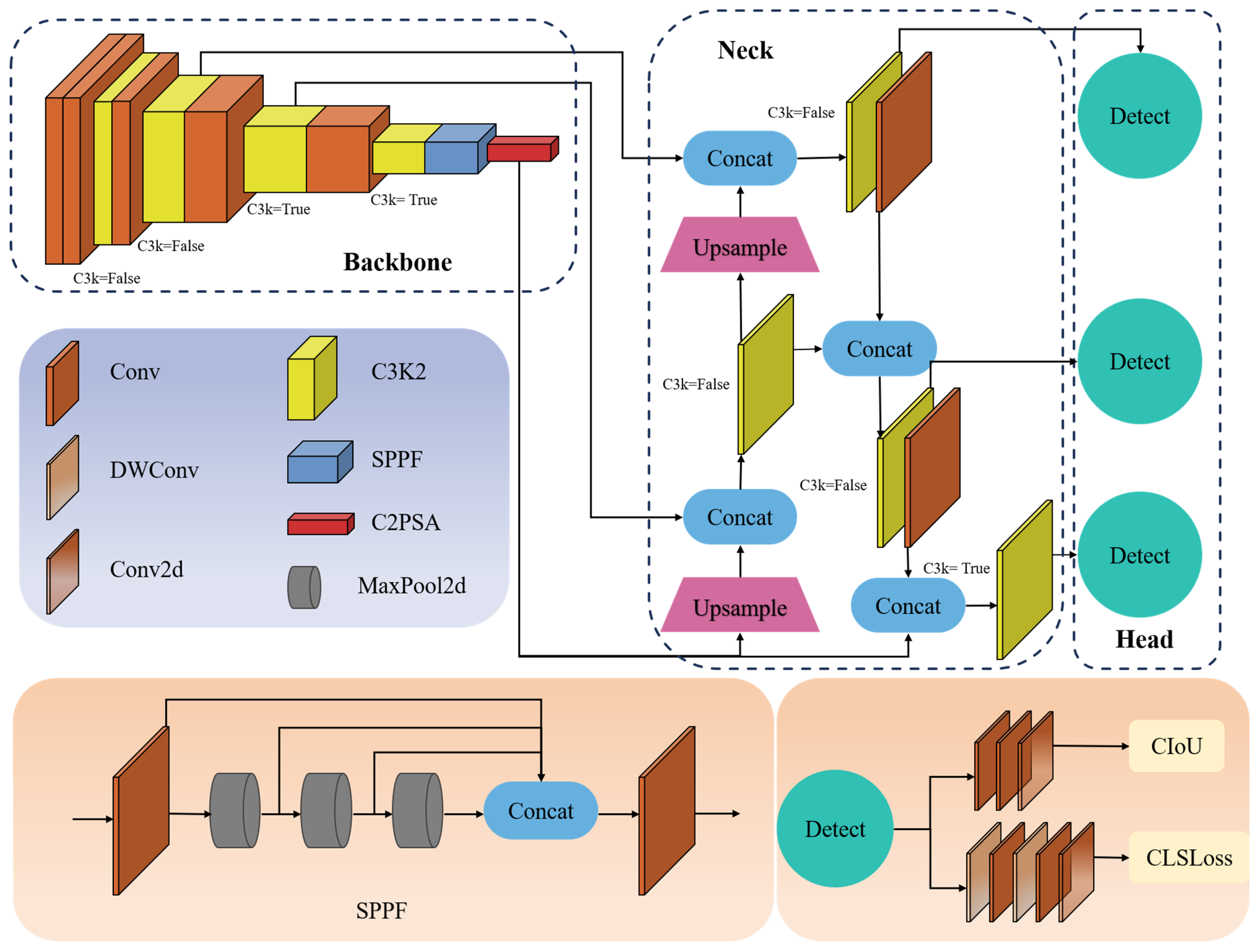
Figure 1.
The overall framework of YOLOv11.
Figure 1.
The overall framework of YOLOv11.
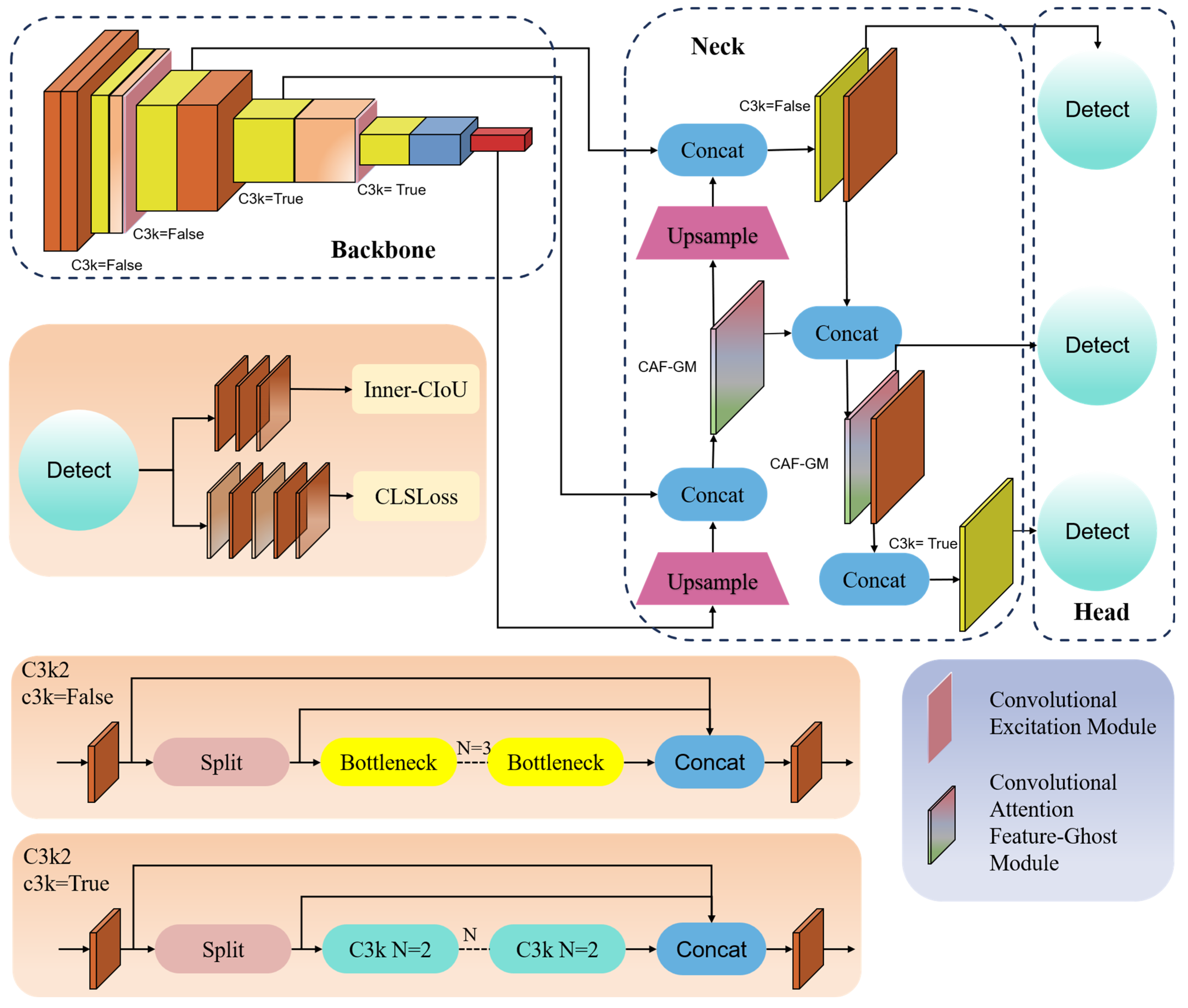
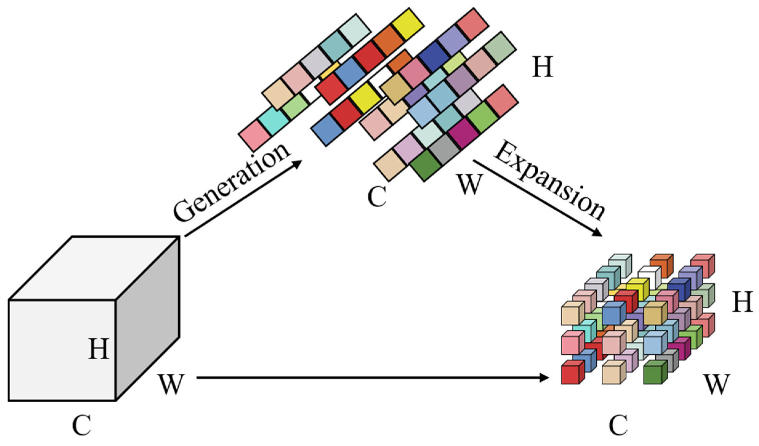
Figure 2.
The overall framework of our ACLC-Detection. Implementation of DSConv and CEM mechanism in the feature extraction network, CAF-GM module for feature enhancement in the neck network, and loss function optimization for enhanced details.
Figure 2.
The overall framework of our ACLC-Detection. Implementation of DSConv and CEM mechanism in the feature extraction network, CAF-GM module for feature enhancement in the neck network, and loss function optimization for enhanced details.
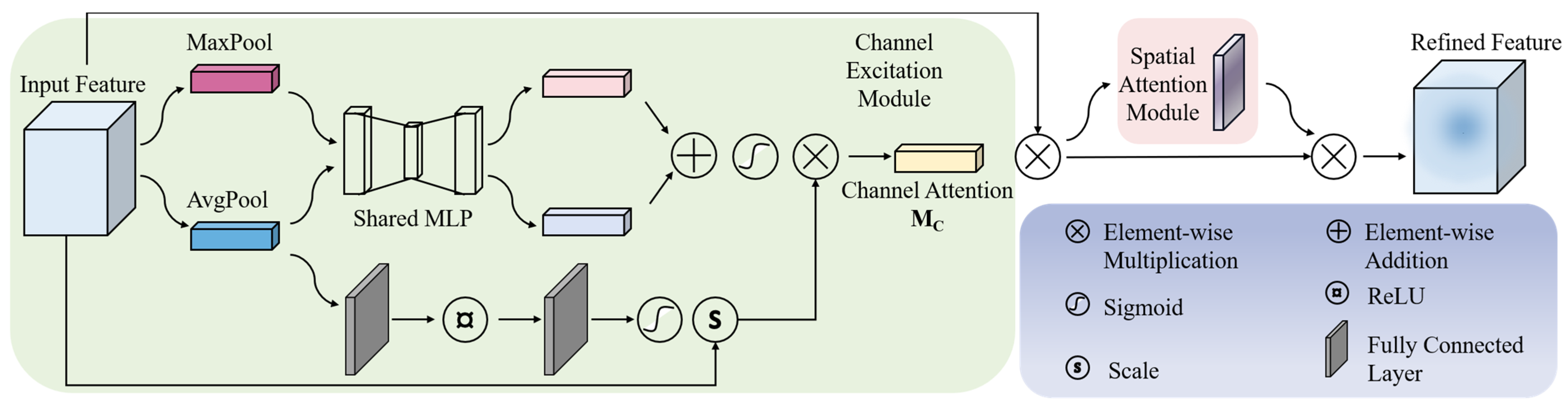
Figure 3.
The schematic diagram of the CE Module.
Figure 3.
The schematic diagram of the CE Module.
Figure 4.
The schematic diagram of the depthwise separable convolution module.
Figure 4.
The schematic diagram of the depthwise separable convolution module.
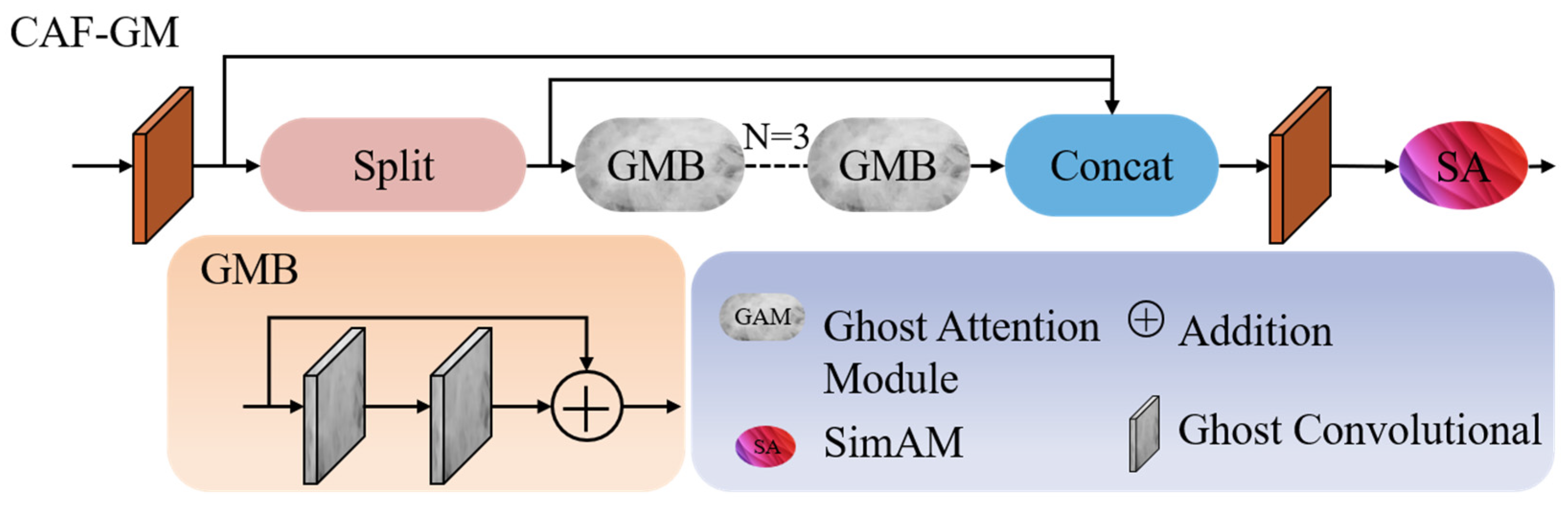
Figure 5.
The schematic diagram of the CAF-GM module.
Figure 5.
The schematic diagram of the CAF-GM module.
Figure 6.
The Ghost module.
Figure 6.
The Ghost module.
Figure 7.
The SimAM module.
Figure 7.
The SimAM module.
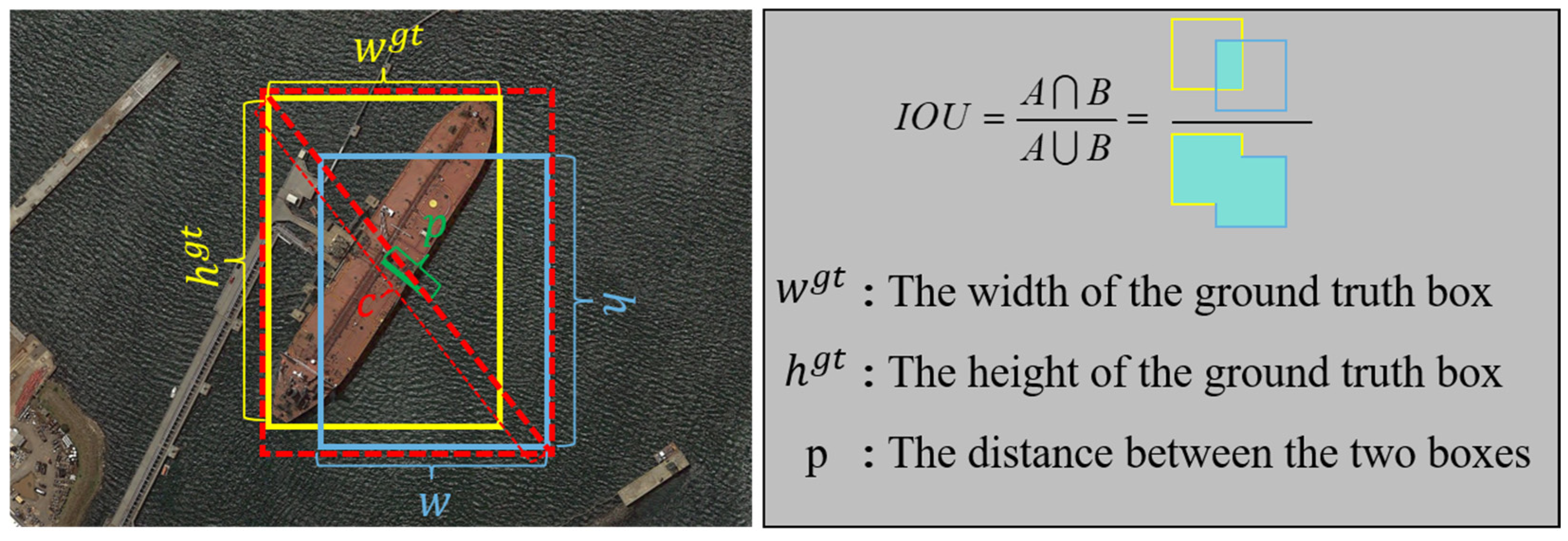
Figure 8.
A visual representation of CIOU and IoU.
Figure 8.
A visual representation of CIOU and IoU.
Figure 9.
A visual representation of Inner-CIoU.
Figure 9.
A visual representation of Inner-CIoU.
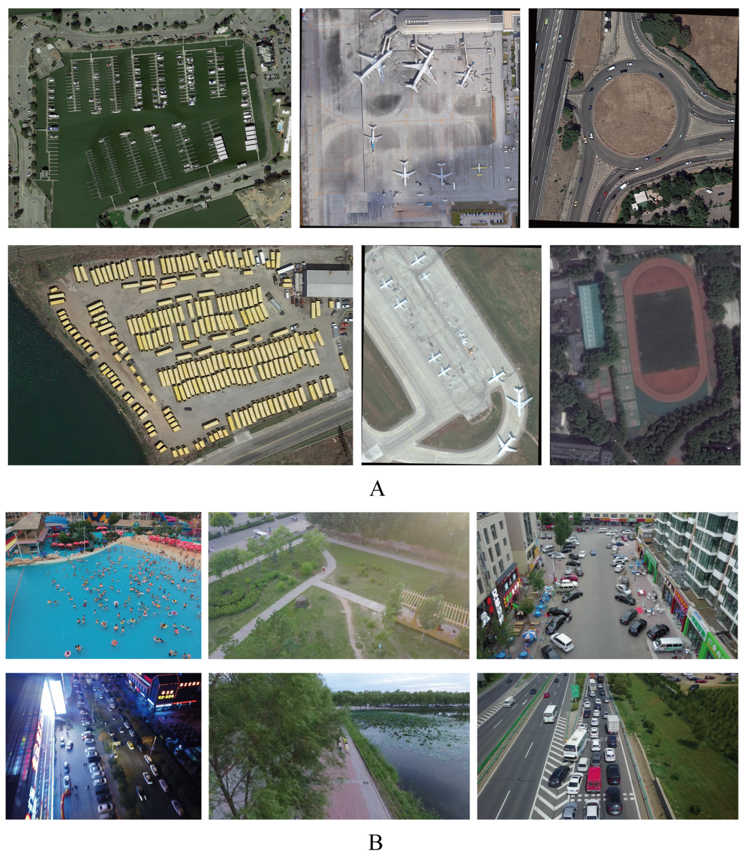
Figure 10.
(A,B) Sample scene images from the dataset. (A) Image from the DOTA dataset. (B) Image from the VisDrone2019 dataset.
Figure 10.
(A,B) Sample scene images from the dataset. (A) Image from the DOTA dataset. (B) Image from the VisDrone2019 dataset.
Figure 11.
Relevant statistics of the dataset (A,B). Part (A) shows the number and average area of various types of targets in the DOTA and VisDrone2019 datasets on the left and right sides, respectively. Part (B) shows the classification of targets in the DOTA and VisDrone2019 datasets based on pixel length and width on the left and right sides, respectively.
Figure 12.
Comparison of PR curves based on the DOTA dataset. The left side shows the results of the original model, while the right side shows the results of the model presented in this paper.
Figure 12.
Comparison of PR curves based on the DOTA dataset. The left side shows the results of the original model, while the right side shows the results of the model presented in this paper.
Figure 13.
Comparison of PR curves based on the VisDrone2019 dataset. The left side shows the results of the original model, while the right side shows the results of the model presented in this paper.
Figure 13.
Comparison of PR curves based on the VisDrone2019 dataset. The left side shows the results of the original model, while the right side shows the results of the model presented in this paper.
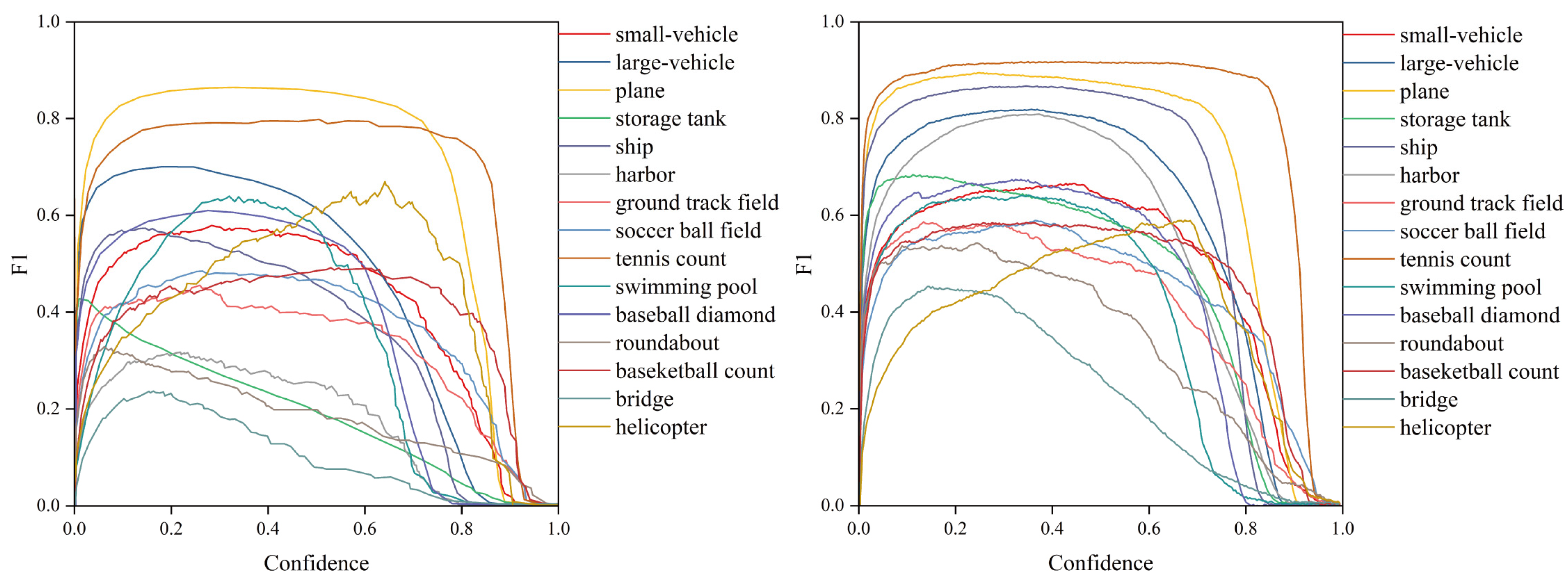
Figure 14.
Comparison of F1 curves based on the DOTA dataset. The left side shows the results of the original model, while the right side shows the results of the model presented in this paper.
Figure 14.
Comparison of F1 curves based on the DOTA dataset. The left side shows the results of the original model, while the right side shows the results of the model presented in this paper.
Figure 15.
Comparison of F1 curves based on the VisDrone2019 dataset. The left side shows the results of the original model, while the right side shows the results of the model presented in this paper.
Figure 15.
Comparison of F1 curves based on the VisDrone2019 dataset. The left side shows the results of the original model, while the right side shows the results of the model presented in this paper.
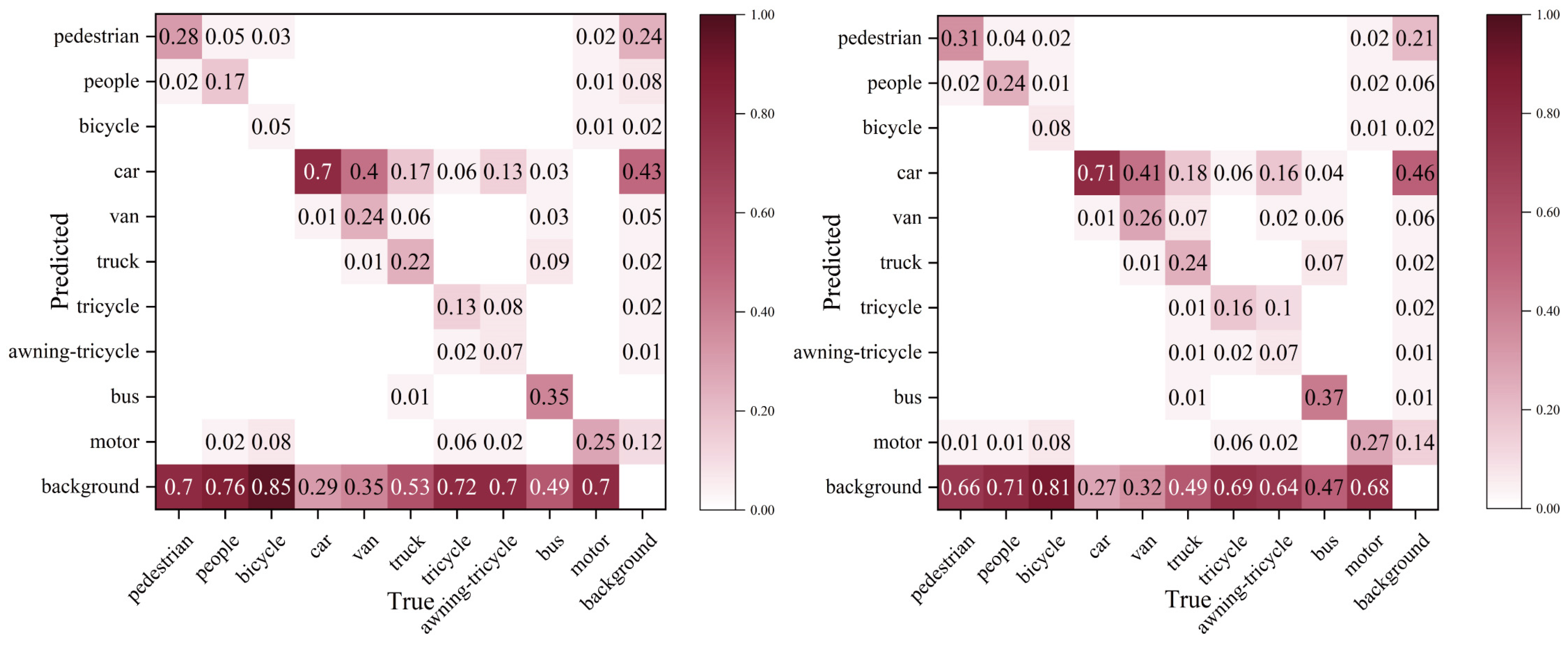
Figure 16.
Based on the confusion matrix diagram of the DOTA dataset, the left side shows the results of the original model, while the right side shows the results of the improved model.
Figure 16.
Based on the confusion matrix diagram of the DOTA dataset, the left side shows the results of the original model, while the right side shows the results of the improved model.
Figure 17.
Based on the confusion matrix diagram of the VisDrone2019 dataset, the left side shows the results of the original model, while the right side shows the results of the improved model.
Figure 17.
Based on the confusion matrix diagram of the VisDrone2019 dataset, the left side shows the results of the original model, while the right side shows the results of the improved model.
Figure 18.
Comparison and analysis of AP50 values. The left subplot shows the results based on the DOTA dataset, while the right subplot shows the results based on the VisDrone2019 dataset.
Figure 18.
Comparison and analysis of AP50 values. The left subplot shows the results based on the DOTA dataset, while the right subplot shows the results based on the VisDrone2019 dataset.
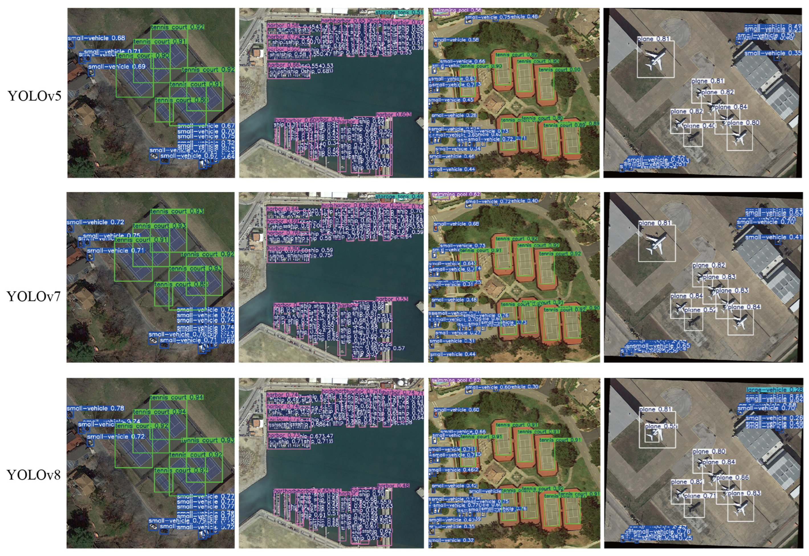
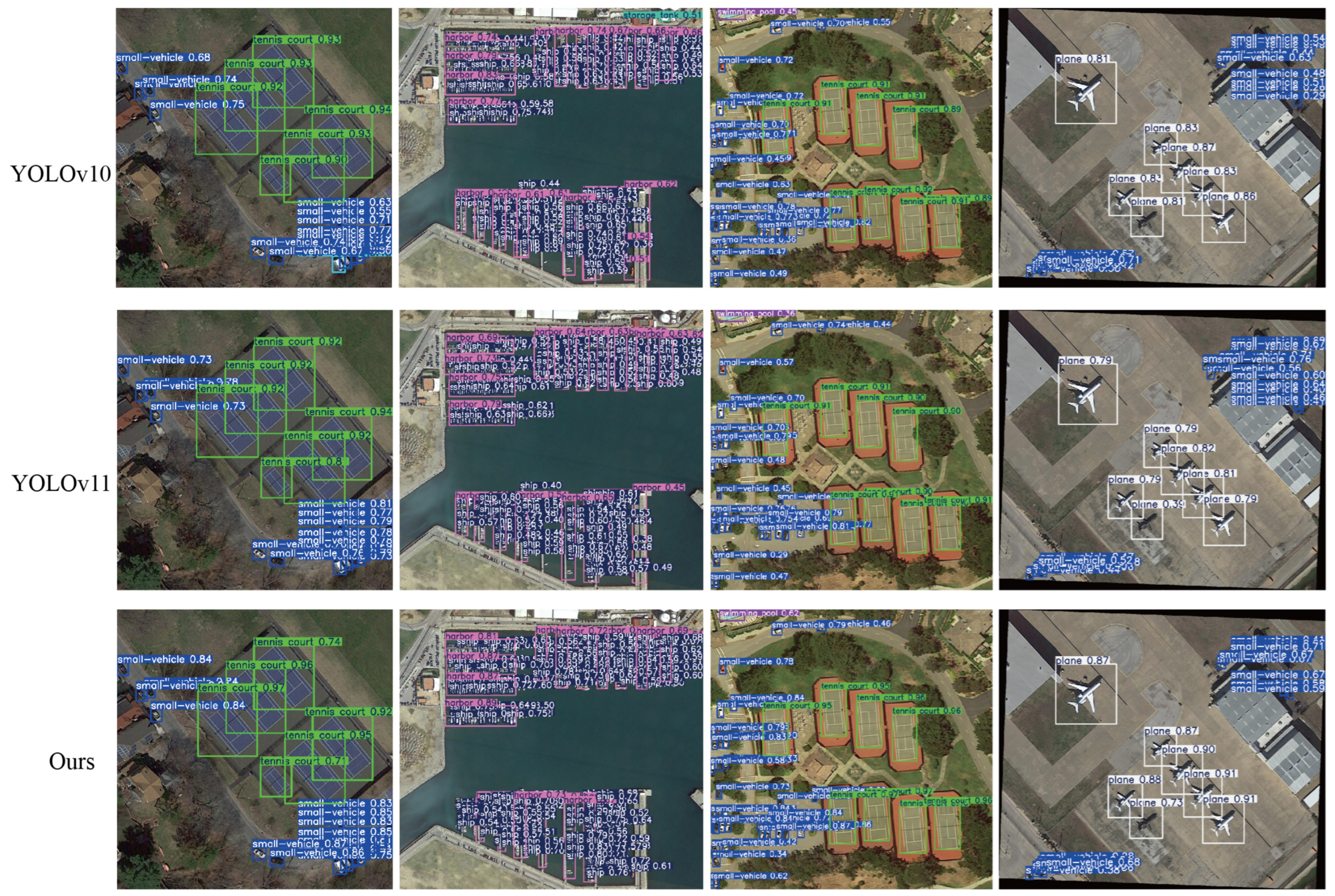
Figure 19.
Analysis of the visualization results based on the DOTA dataset.
Figure 19.
Analysis of the visualization results based on the DOTA dataset.
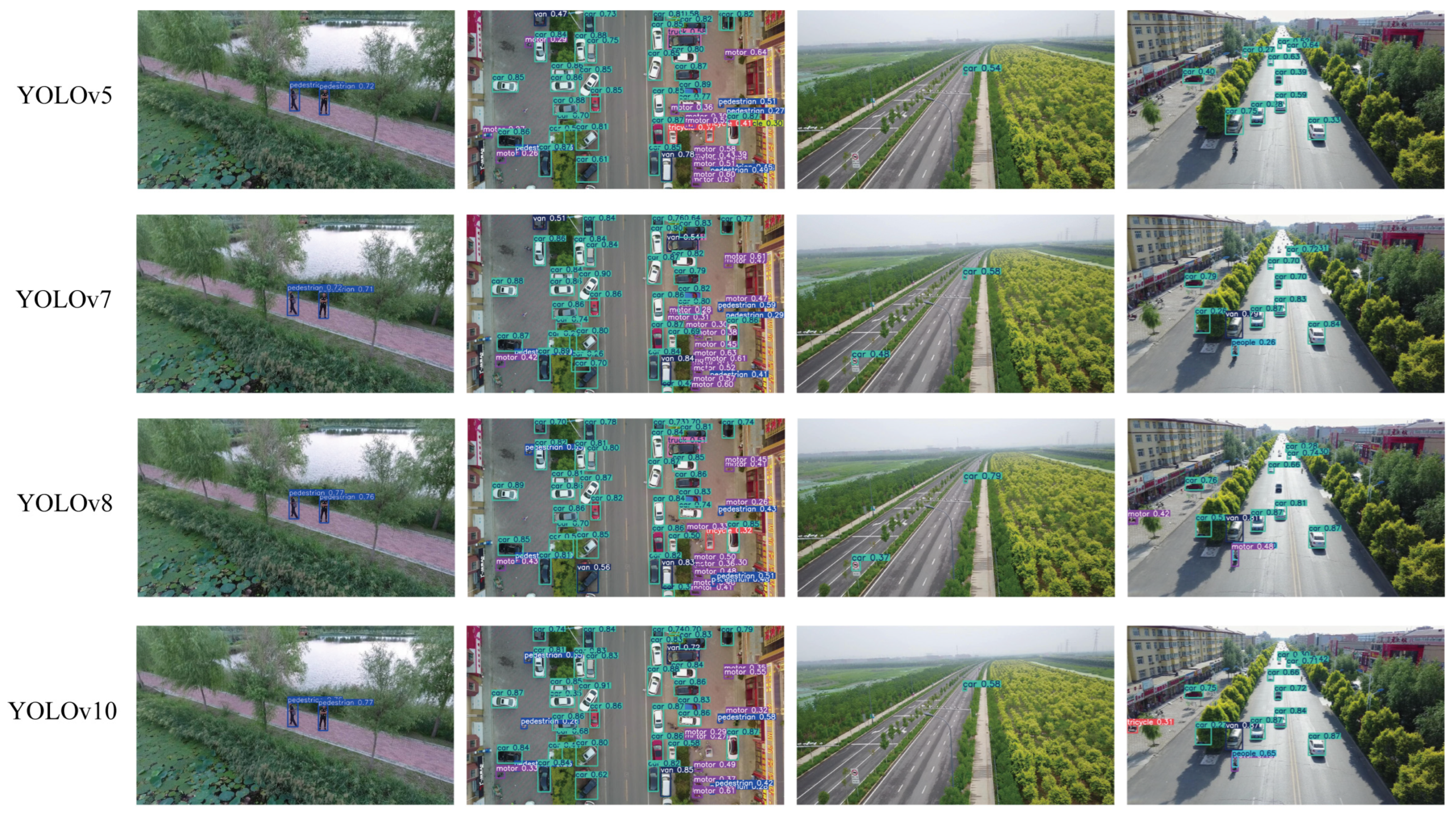
Figure 20.
Analysis of the visualization results based on the VisDrone2019 dataset.
Figure 20.
Analysis of the visualization results based on the VisDrone2019 dataset.
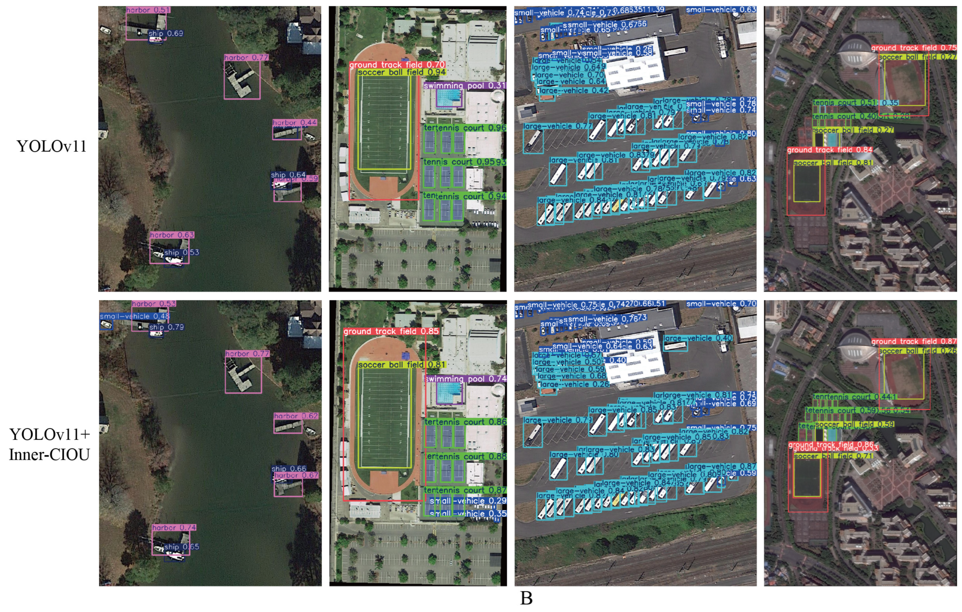
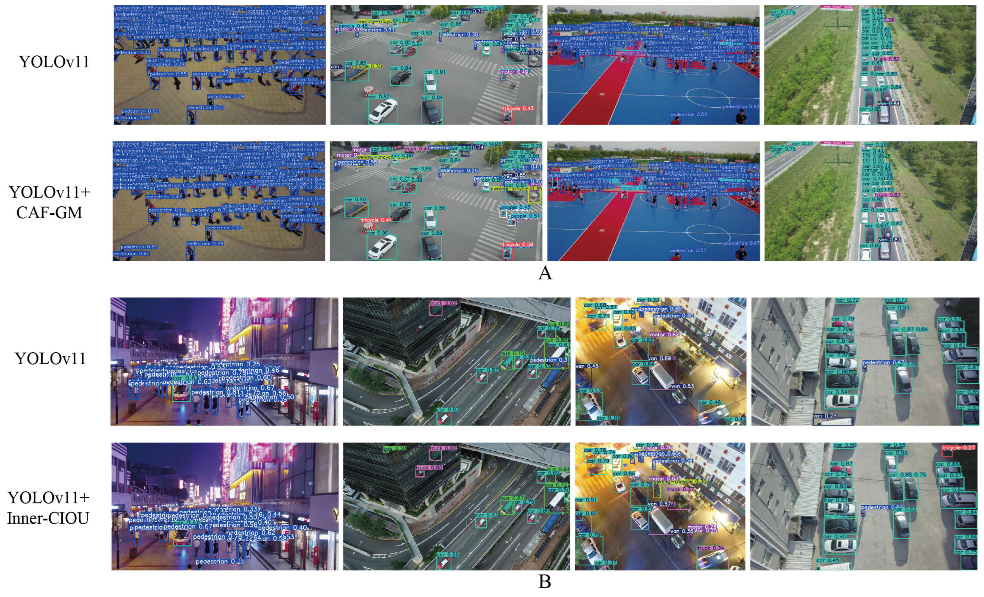
Figure 21.
Visualization results of ablation experiments on the DOTA dataset, where Part (A) shows the results with the introduction of the CAF-GM module, and Part (B) shows the results with the introduction of the Inner-CIOU loss function.
Figure 21.
Visualization results of ablation experiments on the DOTA dataset, where Part (A) shows the results with the introduction of the CAF-GM module, and Part (B) shows the results with the introduction of the Inner-CIOU loss function.
Figure 22.
Visualization results of ablation experiments on the VisDrone2019 dataset, where Part (A) shows the results with the introduction of the CAF-GM module, and Part (B) shows the results with the introduction of the Inner-CIOU loss function.
Figure 22.
Visualization results of ablation experiments on the VisDrone2019 dataset, where Part (A) shows the results with the introduction of the CAF-GM module, and Part (B) shows the results with the introduction of the Inner-CIOU loss function.
Table 1.
Setup and training environment.
Table 1.
Setup and training environment.
| Parameter | Configuration |
|---|
| CPU model | Intel Core i7-9700k |
| GPU model | NVIDIA GeForce RTX 3090Ti |
| Platform | Ubuntu 18.04 LTS 64-bits |
| Deep Learning Architecture | PyTorch1.9.1 |
| GPU Acceleration Device | CUDA10.2 |
| Programming Environment | PyCharm2024.2.4 |
| Scripting System | Python3.8 |
| Neural Network Processing Unit | CUDNN7.6.5 |
Table 2.
Hyperparameter settings.
Table 2.
Hyperparameter settings.
| Parameter | Configuration |
|---|
| Neural network optimizer | SGD |
| Learning rate | 0.001 |
| Training epochs | 200 |
| Momentum | 0.937 |
| Batch size | 16 |
| Weight decay | 0.0005 |
Table 3.
Comparative analysis with other models on the DOTA dataset.
Table 3.
Comparative analysis with other models on the DOTA dataset.
| Method | Param. | FLOPs | mAP | mAP50 | mAP75 | mAPS | mAPM | mAPL |
|---|
| Multi-stage detectors | Fast R-CNN | 46.57 | 88.45 | 37.6 | 51.8 | 43.1 | 22.2 | 35.4 | 36.9 |
| Faster R-CNN | 43.12 | 61.34 | 41.8 | 49.6 | 46.3 | 28.4 | 39.1 | 44.1 |
| Cascade R-CNN | 65.95 | 75.62 | 46.3 | 52.7 | 46.2 | 33.5 | 42.8 | 46.9 |
| RepPoints | 37.43 | 33.74 | 44.6 | 52.8 | 46.1 | 32.3 | 44.7 | 49.2 |
| One-stage detectors | FNI-DETR | 41.58 | 105.42 | 48.1 | 64.3 | 56.8 | 43.5 | 61.2 | 64.5 |
| WDFS-DETR | 19.49 | 53.65 | 48.8 | 66.2 | 58.5 | 45.7 | 64.1 | 63.5 |
| YOLOv5 | 6.97 | 8.45 | 44.3 | 49.8 | 42.4 | 31.6 | 44.6 | 43.5 |
| YOLOv7 | 6.17 | 6.54 | 49.8 | 57.4 | 45.8 | 44.7 | 59.1 | 57.4 |
| YOLOv8 | 6.25 | 8.76 | 48.2 | 66.4 | 57.9 | 45.7 | 63.8 | 62.1 |
| YOLOv10 | 5.59 | 6.73 | 47.3 | 64.5 | 52.6 | 44.2 | 59.4 | 60.9 |
| YOLOv11 | 5.35 | 6.52 | 48.1 | 65.9 | 58.4 | 43.9 | 64.3 | 64.5 |
| ACLC-Detection | 4.47 | 5.28 | 49.8 | 67.1 | 59.4 | 46.3 | 64.7 | 63.9 |
Table 4.
Comparative analysis with other models on the VisDrone2019 dataset.
Table 4.
Comparative analysis with other models on the VisDrone2019 dataset.
| Method | Param. | FLOPs | mAP | mAP50 | mAP75 | mAPS | mAPM | mAPL |
|---|
| Multi-stage detectors | Fast R-CNN | 46.57 | 88.45 | 17.8 | 28.5 | 18.3 | 7.1 | 17.6 | 16.4 |
| Faster R-CNN | 43.12 | 61.34 | 19.2 | 30.8 | 23.1 | 9.8 | 21.7 | 17.1 |
| Cascade R-CNN | 65.95 | 75.62 | 21.8 | 32.4 | 22.6 | 13.5 | 24.2 | 22.1 |
| RepPoints | 37.43 | 33.74 | 24.7 | 32.5 | 23.9 | 16.2 | 28.9 | 26.5 |
| One-stage detectors | FNI-DETR | 41.58 | 105.42 | 27.9 | 38.4 | 32.5 | 23.7 | 31.3 | 27.5 |
| WDFS-DETR | 19.49 | 53.65 | 30.4 | 38.8 | 32.9 | 24.3 | 33.5 | 27.4 |
| YOLOv5 | 6.97 | 8.45 | 26.3 | 35.8 | 26.4 | 14.2 | 26.4 | 24.8 |
| YOLOv7 | 6.17 | 6.54 | 26.5 | 34.5 | 24.1 | 16.5 | 25.6 | 23.9 |
| YOLOv8 | 6.25 | 8.76 | 28.4 | 36.4 | 30.1 | 18.9 | 28.4 | 25.1 |
| YOLOv10 | 5.59 | 6.73 | 28.6 | 35.9 | 32.3 | 19.4 | 29.1 | 25.2 |
| YOLOv11 | 5.35 | 6.52 | 29.7 | 37.5 | 32.6 | 22.5 | 31.2 | 27.4 |
| ACLC-Detection | 4.47 | 5.28 | 30.6 | 39.2 | 33.1 | 24.6 | 32.9 | 28.7 |
Table 5.
Ablation experiments based on DOTA dataset.
Table 5.
Ablation experiments based on DOTA dataset.
| Mobile | LCM | CEM | CAF-GM | Inner-CIOU | mAP | mAPS | mAPM | mAPL | Param. | FLOPS | FPS |
|---|
| YOLOv11 | -- | -- | -- | -- | 48.1 | 43.9 | 64.3 | 64.5 | 5.35 | 6.52 | 158 |
| | √ | -- | -- | -- | 48.2 | 43.8 | 64.4 | 64.6 | 4.99 | 5.94 | 177 |
| | -- | √ | -- | -- | 48.8 | 44.5 | 65.1 | 64.7 | 5.36 | 6.53 | 151 |
| | -- | -- | √ | -- | 49.2 | 45.7 | 65.6 | 64.6 | 4.82 | 5.85 | 163 |
| | -- | -- | -- | √ | 49.1 | 45.9 | 66.2 | 64.6 | 5.35 | 6.52 | 158 |
| | √ | √ | -- | -- | 48.5 | 45.6 | 65.2 | 64.6 | 5.00 | 5.96 | 165 |
| | -- | √ | √ | -- | 48.9 | 45.4 | 65.6 | 64.7 | 4.83 | 5.86 | 156 |
| | -- | -- | √ | √ | 49.5 | 46.1 | 66.4 | 64.8 | 4.82 | 5.85 | 163 |
| | √ | √ | √ | -- | 49.6 | 45.8 | 66.1 | 64.8 | 4.47 | 5.28 | 183 |
| | -- | √ | √ | √ | 49.5 | 46.1 | 66.5 | 64.9 | 4.83 | 5.86 | 156 |
| | √ | √ | √ | √ | 49.8 | 46.3 | 66.7 | 64.9 | 4.47 | 5.28 | 183 |
Table 6.
Ablation experiments based on the VisDrone2019 dataset.
Table 6.
Ablation experiments based on the VisDrone2019 dataset.
| Mobile | LCM | CEM | CAF-GM | Inner-CIOU | mAP | mAPS | mAPM | mAPL | Param. | FLOPS | FPS |
|---|
| YOLOv11 | -- | -- | -- | -- | 29.7 | 22.5 | 31.2 | 27.4 | 5.35 | 6.52 | 164 |
| | √ | -- | -- | -- | 29.6 | 22.6 | 31.6 | 27.6 | 4.99 | 5.94 | 188 |
| | -- | √ | -- | -- | 30.2 | 23.1 | 32.1 | 27.8 | 5.36 | 6.53 | 153 |
| | -- | -- | √ | -- | 30.3 | 23.8 | 32.4 | 28.6 | 4.82 | 5.85 | 171 |
| | -- | -- | -- | √ | 30.2 | 23.5 | 32.5 | 27.5 | 5.35 | 6.52 | 164 |
| | √ | √ | -- | -- | 30.3 | 23.4 | 32.2 | 27.8 | 5.00 | 5.96 | 171 |
| | -- | √ | √ | -- | 30.2 | 24.1 | 32.5 | 28.4 | 4.83 | 5.86 | 159 |
| | -- | -- | √ | √ | 30.4 | 23.9 | 32.6 | 28.5 | 4.82 | 5.85 | 171 |
| | √ | √ | √ | -- | 30.5 | 23.6 | 32.4 | 28.1 | 4.47 | 5.28 | 195 |
| | -- | √ | √ | √ | 30.4 | 24.2 | 32.7 | 28.6 | 4.83 | 5.86 | 168 |
| | √ | √ | √ | √ | 30.6 | 24.6 | 32.9 | 28.7 | 4.47 | 5.28 | 195 |
Table 7.
Comparison and analysis of three loss functions based on the DOTA dataset.
Table 7.
Comparison and analysis of three loss functions based on the DOTA dataset.
| Loss Function | Precision | Recall | mAP50 | FPS | Applicable Scenarios |
|---|
| Inner-CIOU | 40.6 | 41.3 | 42.6 | 158 | Small targets, multi-scale |
| SIOU | 36.9 | 35.5 | 37.4 | 143 | Directional consistency |
| DIOU-R | 39.1 | 38.7 | 41.8 | 172 | Resource-constrained, shape regularity |


