Soil Organic Matter (SOM) Mapping in Subtropical Coastal Mountainous Areas Using Multi-Temporal Remote Sensing and the FOI-XGB Model

Abstract

Accurate regional-scale mapping of soil organic matter (SOM) is crucial for land productivity management and global carbon pool monitoring. Current remote sensing inversion of SOM faces challenges, including the underutilization of temporal information and low feature selection efficiency. To address these limitations, this study developed an integrated framework combining multi-temporal Landsat imagery, field-measured SOM data, intelligent feature optimization, and machine learning. The framework employs two novel image-processing strategies: the Maximum Annual Bare-Soil Composite (MABSC) method to extract background spectral information and the Multi-temporal Feature Optimization Composite (MFOC) method to capture seasonal and environmental dynamics. These features, along with topographic covariates, were processed using an improved Feature-Optimized and Interpretable XGBoost (FOI-XGB) model for key variable selection and spatial mapping. Validation across two subtropical coastal mountainous regions at different scales in southeastern China demonstrated the framework’s effectiveness and robustness. Key findings include the following: (1) Both the MABSC-derived spectral bands and the MFOC-optimized indices significantly outperformed traditional single-season approaches. Their combined use achieved a moderate SOM inversion accuracy (R² = 0.42–0.44). (2) The FOI-XGB model substantially outperformed traditional feature selection methods (Pearson, SHAP, and CorrSHAP), achieving significant regional R² improvements ranging from 9.72% to 88.89%. (3) The optimal model integrating the MABSC-derived features, MFOC-optimized indices, and topographic covariates attained the highest accuracy (R² up to 0.51). This represents major improvements compared with using topographic covariates alone (R² increase of up to 160.11%) or the combined spectral features (MABSC + MFOC) alone (R² increase of up to 15.91%). This study provides a robust, scalable, and practical technical solution for accurate SOM mapping in complex environments, with significant implications for sustainable land management and carbon monitoring.

1. Introduction

Soil, as the largest terrestrial carbon reservoir on Earth, plays a pivotal role in regulating the global carbon cycle and sustaining ecosystem functions [1]. Soil organic matter (SOM) is not only the dominant form of carbon storage in terrestrial ecosystems [2] but also a key indicator of soil health and fertility [3]. It supports plant growth and influences hydrological processes [4], thereby contributing critically to regional ecological balance and sustainable development [5,6,7]. However, due to complex natural conditions and intensifying anthropogenic activities, SOM exhibits marked spatial heterogeneity [8,9], making large-scale, high-resolution monitoring a pressing scientific and policy-driven priority [6].

Traditional laboratory-based approaches for SOM assessment, while accurate, are often time-consuming, costly, and spatially constrained in representativeness [10]. These limitations hinder their applicability for rapid, dynamic, and comprehensive SOM mapping over broad regions, especially in heterogeneous landscapes [11]. To address these challenges, remote sensing technology has emerged as a powerful tool, offering extensive spatial coverage, efficient data acquisition, and multi-temporal observation capabilities. Among these, multispectral remote sensing has garnered particular attention due to its widespread data availability and appropriate spatial-temporal resolution [12].

The Landsat satellite series, which has provided continuous Earth observations since 1972, offers imagery at a 30 m spatial resolution across key spectral regions, including the visible, near-infrared, and shortwave-infrared bands. This long-term, consistent, and spatially extensive dataset has made Landsat particularly suitable for regional-scale digital soil mapping (DSM), especially for retrieving soil organic matter (SOM) and detecting its gradual changes under relatively stable environmental conditions [13,14]. With the successive launches of Landsat 5, 7, 8, and 9, the program has undergone continuous sensor and calibration improvements, including enhanced spectral resolution, improved radiometric accuracy, and greater geometric consistency. These advances have significantly improved the extraction of bare-soil spectral signals and the construction of multi-temporal SOM prediction models [15,16]. As a result, Landsat data have become deeply integrated into the DSM process, supporting fine-scale SOM mapping, model transferability studies, and long-term soil condition monitoring across diverse landscapes [17].

In addition to Landsat, the Sentinel-2 series (launched by the European Space Agency in 2015) provides a 10 m spatial resolution and frequent revisit intervals (every 5 days), making it highly effective for high-resolution monitoring of dynamic environmental changes [18]. However, despite its higher spatial resolution, Sentinel-2’s relatively short data record (from 2015 onwards) limits its applicability for long-term trend analysis. Furthermore, several studies have indicated that Sentinel-2’s inversion results for SOM may not always outperform those of Landsat [19,20], particularly in regions where soil spectral signals are closely associated with other surface features, such as vegetation cover. Sentinel-2 is a valuable tool for monitoring areas that require frequent data collection, and its high temporal resolution has great potential for monitoring SOM in the future [21]. Currently, Landsat remains the primary tool for long-term soil organic matter monitoring and trend analysis due to its multi-year continuous datasets and inversion capabilities.

In parallel, an increasing number of studies have emphasized the value of incorporating topographic variables in SOM modeling for complex mountainous regions [22]. Numerous studies have demonstrated that topographic features can effectively support SOM estimation in heterogeneous terrain by capturing terrain-induced spatial variability [23]. In such landscapes, terrain exerts significant influence on soil formation processes, microclimates, and hydrological patterns, all of which affect SOM distribution. While the impact of topography may be negligible in flat or small-scale regions, its inclusion becomes essential when focusing on hilly or mountainous environments [24,25]. Therefore, clarifying the geographic context and highlighting the relevance of topographic factors enhance the scientific rigor and contextual accuracy of variable selection in DSM frameworks.

Nevertheless, several technical challenges continue to constrain accurate SOM retrieval from multispectral imagery: complex surface conditions—such as vegetation cover [26], seasonal phenological shifts [27], and dynamic soil moisture variations [28]—substantially distort spectral signals, while frequent cloud and shadow interference [29] further complicates the extraction of stable, pure bare-soil spectra. Consequently, it is imperative to develop methods that (1) effectively extract high-quality bare-soil information from long-term imagery with minimal interference from vegetation, soil moisture, and cloud cover [30,31]; (2) optimally leverage multi-temporal features—rather than simply stacking images, which can introduce noise and redundant information [32]—to balance data volume against model accuracy and reliably reflect SOM accumulation dynamics [21,33]; and (3) identify robust, interpretable predictor combinations from high-dimensional datasets—comprising raw spectral bands, derived indices, and auxiliary environmental variables [34]—to mitigate multicollinearity, prevent overfitting, and enhance model generalization [35,36].

In response, this study proposes a comprehensive framework for SOM retrieval using long-term Landsat imagery, integrating remote sensing feature extraction, variable selection, and modeling. Specifically, the framework incorporates the following techniques: (1) A SOM remote sensing feature extraction technique: A composite approach, combining the Maximum Annual Bare-Soil Composite (MABSC) method and the Multi-temporal Feature Optimization Composite (MFOC) method, is used to extract optimal annual bare-soil features and identify temporally stable predictors. (2) A SOM feature selection technique: FOI-XGB (Feature-Optimized and Interpretable XGBoost), a variable selection method, integrates XGBoost for high-accuracy prediction, SHAP for model interpretability, and RFECV for robust variable elimination via cross-validation. (3) A SOM remote sensing modeling and mapping technique: XGBoost-based SOM inversion and high-resolution mapping use the selected variable subsets.

This research focuses on farmlands in two subtropical coastal mountainous areas of southeastern China—Fuzhou City and the lower reaches of the Mulan River in Putian City—spanning different spatial scales. By generating optimized predictor sets and developing transferable models, this study aims to construct a reliable framework for SOM mapping in complex terrain environments. The findings will contribute to enhanced regional land resource management and support global efforts in carbon stock assessment.

2. Materials and Methods

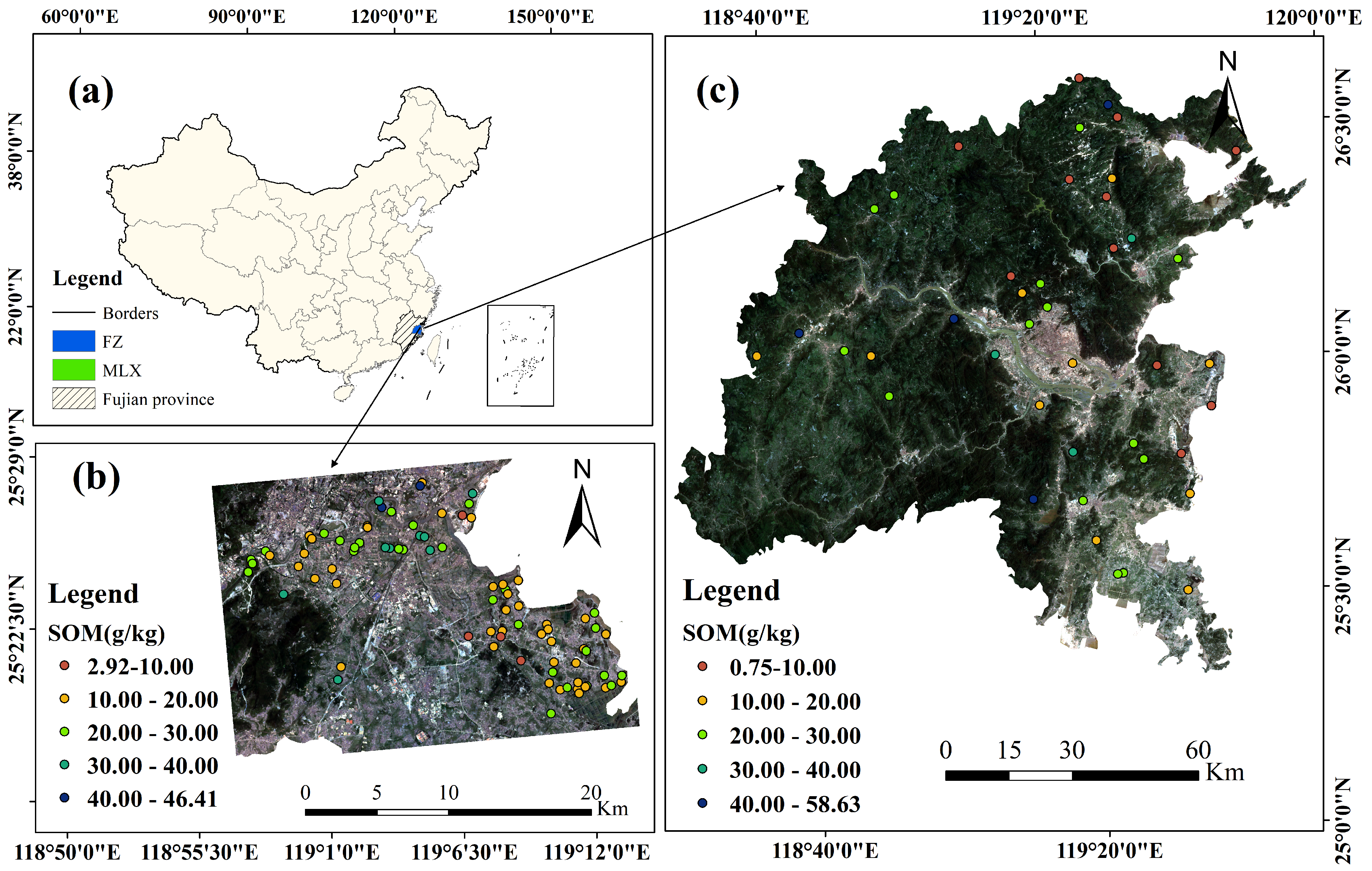
2.1. Study Area

In this study, Fuzhou City (FZ; 118°08′–120°31′E, 25°15′–26°29′N; area: 11,597 km²) and the lower reaches of the Mulan River in Putian City (MLX; 118°57′–119°15′E, 25°17′–25°27′N; area: 538 km²), both located on the southeast coast of China, were selected as the study areas. FZ has a subtropical maritime monsoon climate and is characterized by a hilly and mountainous landscape. The dominant soil types in FZ include acidic red and reddish soils, with some rice soils. MLX is located approximately 115 km south of FZ. It has similar climatic conditions but a smaller spatial scale, and its soil is mainly composed of rice soils and saline soils [37]. A total of 41 and 83 surface soil samples (0–20 cm) were collected from FZ and MLX, respectively (Figure 1). Although both regions are situated in the southeastern coastal zone, they differ significantly in spatial scale. Their selection aimed to evaluate the stability and regional applicability of the proposed SOM inversion method under different spatial conditions.

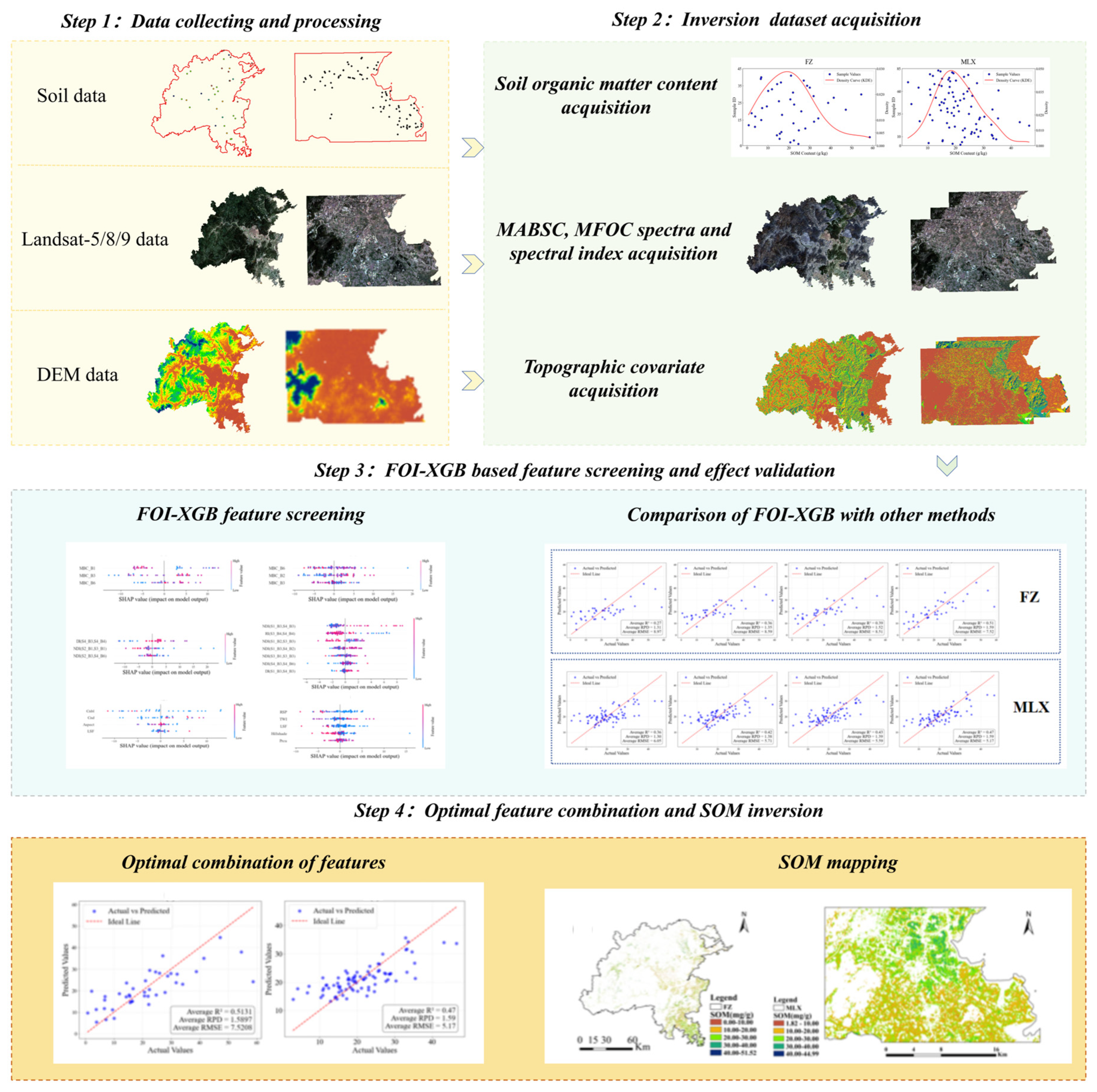
2.2. Research Methods

This study integrated remote sensing time-series analysis with machine learning methods to evaluate model stability across two typical regions along the southeast coast of China under different temporal (FZ: 2012; MLX: 2017, 2023) and spatial scales (FZ: 11,597 km²; MLX: 538 km²). The technical workflow (Figure 2) comprised four key steps: (1) Data acquisition: SOM content data were obtained through field sampling across the study area, followed by laboratory analysis. Landsat images and digital elevation model (DEM) data were acquired from Google Earth Engine for the study area and period of interest. (2) Extraction of SOM remote sensing feature variables: Using the Google Earth Engine platform, optimal bare-soil images were obtained through the Maximum Annual Bare-Soil Composite (MABSC) method. Spectrally stable phase-combination images were selected by applying the Kauth–Thomas (K–T) transform combined with the Multi-temporal Feature Optimization Composite (MFOC) method, yielding a de-noised, high-quality soil information dataset. Topographic covariates were derived from the DEM data using spatial analysis techniques. (3) Feature selection for SOM inversion: Spectral indices (NDI/RI/DI), topographic factors, and multi-temporal spectral features were integrated. The FOI-XGB model, which combines XGBoost prediction, SHAP-based interpretability, and Recursive Feature Elimination with Cross-Validation (RFECV), was employed for feature optimization. (4) SOM inversion and mapping: An inversion model was constructed using the XGBoost algorithm, with model accuracy assessed through tenfold cross-validation.

Through temporal image optimization and intelligent feature selection, the proposed method enables regional validation across temporal and spatial scales, thereby improving the accuracy, robustness, and regional adaptability of SOM inversion.

2.3. Soil Sampling and SOM Analysis

Surface soil samples (0–20 cm) were collected in late July 2012 at FZ (41 sites), corresponding to the post-harvest period of early-season rice when cropland was relatively bare. At MLX, sampling was conducted in late October 2017 and 2023 (83 sites total: 31 in 2017 and 52 supplementary sites from China’s 2023 National Soil Census), aligning with the post-harvest period of late-season rice when farmland was also relatively bare. Leveraging the relative stability of soil organic matter over 5–10-year timescales, the two-phase MLX datasets were merged to construct an enhanced composite dataset. Sampling followed a standardized protocol: Within a 30 m × 30 m grid system covering the study area, a 1 m × 1 m quadrat was established centered on each grid node. Sub-samples from five points (four corners and center) were composited into a single homogenized sample. All locations were georeferenced using handheld GPS (horizontal accuracy < 3 m), strictly adhering to the single-pixel-per-sample principle to ensure spatial co-registration with 30 m resolution remote sensing data.

All soil samples were air-dried, ground, and passed through a 2 mm sieve. For the FZ samples, soil organic matter (SOM) content (g/kg) was determined using the potassium dichromate oxidation method [38]. For the MLX samples, due to technological advancements and sulfuric acid regulations, soil organic carbon (SOC) content (g/kg) was measured using an Elementar Vario MAX elemental analyzer, which employs dry combustion at 1200 °C with NDIR detection—a method known for its superior precision and accuracy, immunity to reducing substances, and enhanced sensitivity for low-SOM soils. This method offers high-throughput automation, improved safety by avoiding toxic chromates (though acid pretreatment remains), and compliance with international standards [39,40] (ISO 10694). The SOM content was derived by multiplying the SOC by a standard conversion factor of 1.724 [41].

2.4. Soil Remote Sensing Feature Extraction

In this study, a combination of direct and indirect remote sensing approaches was employed to retrieve soil organic matter (SOM) using long-term time-series satellite imagery. The direct approach was implemented via the Maximum Annual Bare-Soil Composite (MABSC) method, which extracts spectral information from pixels representing the most exposed bare-soil conditions during each year. This allows for direct characterization of SOM-related reflectance signals while minimizing interference from vegetation and moisture. In parallel, the Multi-temporal Feature Optimization Composite (MFOC) method served as an indirect approach, selecting representative surface states across multiple seasons. This method is based on the premise that vegetation dynamics over time can reflect the underlying soil fertility and SOM levels. By integrating both MABSC and MFOC, the framework combines the strengths of direct spectral observation and vegetation-mediated inference, enhancing the robustness of SOM retrieval across varied surface conditions.

All remote sensing data acquisition and processing were conducted on the Google Earth Engine (GEE) platform, which offers a scalable, cloud-based environment for planetary-scale geospatial analysis [41]. Due to the persistent cloud cover, shadows, and vegetation in the study areas—factors that complicate the retrieval of soil reflectance signals—a per-pixel compositing strategy was employed to generate high-quality surface reflectance imagery. The MABSC and MFOC procedures were applied within GEE to construct temporally stable and spectrally pure datasets for soil organic matter (SOM) inversion. Following the assumption that SOM remains relatively stable over a five-year period, image datasets were constructed for different regions based on corresponding temporal windows. For FZ, where soil sampling occurred once in late July 2012, Landsat 5/7/8 surface reflectance imagery from 2010 to 2014 was utilized. For MLX, where sampling took place in late October in both 2017 and 2023, a composite image dataset was assembled using Landsat 8/9 surface reflectance data spanning the period from 2016 to 2024. All imagery was sourced from the USGS Level 2 Collection 2 Tier 1 products, which are atmospherically corrected and radiometrically calibrated, ensuring the quality required for accurate SOM estimation.

Six key spectral bands from Landsat 5, 8, and 9 were selected: blue (Blue), green (Green), red (Red), near-infrared (NIR), shortwave-infrared 1 (SWIR1), and shortwave-infrared 2 (SWIR2). For consistency in the subsequent analysis and model development, these bands were uniformly renamed as B1 through B6, respectively.

2.4.1. Maximum Annual Bare-Soil Composite (MABSC)

Building upon previous studies that utilized bare-soil composites for soil property mapping [42], this study proposed an improved method for generating high-quality bare-soil imagery. Landsat imagery was processed on the GEE platform by first collecting all available images from the target and adjacent years over the study area, followed by cloud masking. The Bare-Soil Index (BSI; Equation (1)) was then calculated for each valid pixel. To accurately capture the maximum bare-soil conditions while minimizing interference from clouds, shadows, and water bodies, a filtering process was applied to the BSI values of each pixel, retaining the top 90–95% of values and computing the median to generate a noise-reduced composite. The resulting MABSC image—containing the B1–B6 bands—represents the optimal bare-soil surface reflectance for the given time period, providing cleaner and more reliable soil spectral information for SOM mapping.

$$BSI=\left[(SWIR+RED)-(NIR+BLUE)\right]/\left[(SWIR+RED)+(NIR+BLUE)\right]$$

(1)

where SWIR, NIR, RED, and BLUE represent the reflectance values of the shortwave-infrared, near-infrared, red, and blue bands, respectively; and BSI is the Bare-Soil Index.

2.4.2. Multi-Temporal Feature Optimization Composite (MFOC)

The Multi-temporal Feature Optimization Composite (MFOC) method was implemented on the GEE platform. For the two study areas, FZ (2010–2014) and MLX (2016–2024), complete monthly Landsat image series from January to December in the sampling year and adjacent years were acquired. To ensure the validity of the monthly data, a cloud-masked image pyramid was constructed for each month.

Subsequently, Kauth–Thomas (K–T) transformations (Equations (2) and (3)) were applied to the monthly images in each study area to compress the multispectral data and extract three physically interpretable components: brightness, greenness, and wetness.

$$L\mathrm{andsat}5\_KT=\left[\begin{array}{cccccc}0.3037& 0.2793& 0.4743& 0.5585& 0.5082& 0.1863\\ -0.2848& -0.2435& -0.5436& 0.7243& 0.0840& -0.1800\\ 0.1509& 0.1973& 0.3279& 0.3406& -0.7112& -0.4572\end{array}\right]\cdot \left[\begin{array}{l}B1\\ B2\\ B3\\ B4\\ B5\\ B6\end{array}\right]$$

(2)

$$L\mathrm{andsat}8/9\_KT=\left[\begin{array}{cccccc}0.3029& 0.2786& 0.4733& 0.5599& 0.5080& 0.1872\\ -0.2841& -0.2430& -0.5424& 0.7276& 0.0713& -0.1608\\ 0.1511& 0.1973& 0.3283& 0.3407& -0.7177& -0.4559\end{array}\right]\cdot \left[\begin{array}{l}B1\\ B2\\ B3\\ B4\\ B5\\ B6\end{array}\right]$$

(3)

where B* denotes the renamed bands of Landsat 5/8/9.

After extracting the brightness, greenness, and wetness components from the K–T transformations of the monthly imagery for both study areas, the corresponding K–T values at the sampling points were statistically analyzed. By comparing the K–T component values across different months, images from multiple months with similar values across all three components were selected and combined to form temporal composites. Based on feature similarity and the local climatic conditions of FZ and MLX, the year was divided into four seasonal periods: S1 (March–May), S2 (June–August), S3 (September–November), and S4 (December–February). For each seasonal period, composite images were generated using the B1–B6 spectral bands. Accordingly, the Multi-temporal Feature Optimization Composite (MFOC) processing procedure involved (1) applying K–T transformations to all annual Landsat images; (2) categorizing the images into seasonal groups based on similarity of K–T component values; and (3) compositing seasonal imagery to produce the final MFOC composite image.

2.4.3. Spectral Index

Previous studies have demonstrated that incorporating spectral indices, especially those reflecting vegetation dynamics or surface conditions, can improve the accuracy of SOM prediction through indirect estimation, particularly when using multispectral data with limited spectral resolution [19,43]. Based on this understanding, the present study constructed six distinct feature datasets to systematically evaluate the effectiveness of both direct observation (based on bare-soil reflectance) and indirect observation (influenced by vegetation). These datasets included (1) the single-temporal imagery (STI) band dataset, (2) the STI spectral index dataset, (3) the MABSC band dataset, (4) the MABSC spectral index dataset, (5) the MFOC band dataset, and (6) the MFOC spectral index dataset.

The STI datasets were derived from seasonally composited Landsat images selected based on the Kauth–Thomas (K–T) transformation results and local cloud-interference patterns. Specifically, the STI image for FZ was generated by compositing imagery from June to August for the years 2010–2014, while the STI image for MLX was generated by compositing imagery from September to November for the years 2016– 2024.

All spectral indices, including the Normalized Difference Index (NDI, Equation (4)), Ratio Index (RI, Equation (5)), and Difference Index (DI, Equation (6)), were computed through pairwise combinations of Landsat surface reflectance bands within the MABSC, MFOC, and STI composites. Collectively, these six datasets represent a comprehensive set of spectral features capturing both direct (bare-soil) and indirect (vegetation-modulated) signals, providing a robust foundation for subsequent feature selection and SOM modeling.

$$NDI=(P_{\mathrm{i}}-P_{\mathrm{j}})/(P_{\mathrm{i}}+P_{\mathrm{j}})$$

(4)

$$RI=P_{\mathrm{i}}/P_{\mathrm{j}}$$

(5)

$$DI=P_{\mathrm{i}}-P_{\mathrm{j}}$$

(6)

where NDI denotes the Normalized Difference Index, RI denotes the Ratio Index, and DI denotes the Difference Index. P_i and P_j represent the reflectance values of bands i and j, respectively.

2.5. Topographic Covariates

This study obtained global topographic data from the Shuttle Radar Topography Mission (SRTM) via the GEE platform. The SRTM project, jointly conducted by the National Aeronautics and Space Administration (NASA) and the National Geospatial-Intelligence Agency (NGA) of the U.S. Department of Defense, is a global terrain-mapping program. In February 2000, radar systems onboard the space shuttle collected data to generate a high-precision digital elevation model (DEM) covering most of the Earth’s land surface [44]. Based on the 30 m SRTM DEM data, a series of key topographic covariates (TCs) was derived. These variables (

Table 1. Topographically derived variables.

Attribute	Definition	Derivative Attribute Meaning
Elevation	Elevation	Height of a point on the Earth’s surface relative to sea level
Slope	Slope	Degree of inclination of the terrain surface
Aspect	Aspect	slope orientation
Hillshade	Hillshade	Light conditions on topographic surfaces
TWI	Topographic Wetness Index	Topography’s ability to accumulate water
TCA	Total Catchment Area	Size of the catchment area upstream of a point
Plcu	Plan Curvature	Degree of curvature of the terrain in the horizontal direction
Prcu	Profile Curvature	Degree of vertical curvature of the terrain
Cnbl	Channel Network Base Level	Lowest point of the river network
Cnd	Channel Network Distance	Distance from a point to the nearest river
Cld	Closed Depressions	Low-lying areas in the terrain
CNI	Convergence Index	Topography’s ability to converge water flows
LSF	LS Factor	Combined effects of slope gradient and slope length on soil erosion
VD	Valley Depth	Vertical distance from the valley floor to the surrounding terrain
RSP	Relative Slope Position	Relative position of a point on a slope

) comprehensively characterize the terrain features of the study areas and are crucial for understanding and modeling the environmental factors that influence soil properties [24,25].

2.6. SHAP-XGB

The SHAP-XGB model, which integrates Extreme Gradient Boosting (XGBoost) with SHapley Additive exPlanations (SHAP), aims to construct a high-accuracy and interpretable machine learning framework. XGBoost is an efficient and scalable gradient boosting algorithm [45] that is widely applied in classification and regression tasks due to its outstanding predictive performance (Equation (7)). However, ensemble learning models such as XGBoost are often regarded as “black boxes” because of their internal complexity, making it difficult to interpret their decision-making processes. This lack of transparency limits their applicability in scenarios requiring interpretability and explainability [46].

To address this issue, SHAP values are introduced. Derived from cooperative game theory, SHAP provides a unified and theoretically sound approach for explaining the outputs of any machine learning model (Equation (8)). By assigning a SHAP value to each input feature, SHAP decomposes the model’s output into the contributions of individual features, clearly illustrating the magnitude and direction of each feature’s influence on a given prediction [47].

$$y_i={\displaystyle {\sum }_{k=1}^K{f}_k\left(x_i\right)},f_k\in \mathit{\Gamma },K$$

(7)

where $y_i$ represents the predicted value for the i-th sample; $f_k$ is the k-th decision tree; K is the total number of decision trees; and $\mathit{\Gamma }$ is the set of all decision trees.

$${\varphi }_j={\displaystyle {\sum }_{S\subseteq F\left|\right\{j\}}}{\displaystyle \frac{\left|S\right|!(\left|F\right|-\left|S\right|-1)!}{\left|F\right|!}}(E[f(X)\left|\mathit{do} (X_S=x_S)\right.]-E[f(X)])$$

(8)

where ${\varphi }_{\mathrm{j}}$ is the SHAP value for the j-th feature; S denotes a subset of features; $E[f(X)\left|\mathit{do} (X_S=x_S)\right.]$ is the expected value given that the feature in S takes the value $x_S$; and $E[f(X)]$ is the expected value of all features.

2.7. FOI-XGB

While the SHAP-XGB method is effective for feature selection, it has a key limitation: the number of selected features must be manually specified, introducing subjectivity into the process. To address this issue, this study proposes the FOI-XGB (Feature-Optimized and Interpretable XGBoost) model, which integrates SHAP-XGB with an improved Recursive Feature Elimination (RFE) strategy. Recursive Feature Elimination (RFE) is a model-based feature selection method that recursively eliminates features with the least importance based on their contribution to the model [48]. However, a major drawback of traditional RFE is its inability to automatically determine the optimal number of features. To overcome this limitation, this study adopts the RFECV (Recursive Feature Elimination with Cross-Validation) algorithm (Equation (9)). The advantages of RFECV include the following: (1) using a Random Forest estimator to evaluate feature importance, ensuring robust and stable feature ranking; (2) automatically identifying the optimal number of features through 10-fold cross-validation, avoiding manual intervention; and (3) setting step = 1 to enable fine-grained feature elimination.

$$X_{\mathit{optimal}}={\mathit{max}}^{(t)}\left({\displaystyle \frac{1}{k}}{\displaystyle \sum _{i=1}^k\left(x_{train}^{(t)},y_{train},x_{va{l}_i}^{(t)},y_{va{l}_i}\right)}\right)$$

(9)

where X_optimal represents the final set of selected features by the FOI-XGB model; x^(t) denotes the result at the t-th iteration; Metric is the performance evaluation index; and k is the number of folds in cross-validation.

2.8. SOM Mapping and Evaluation

2.8.1. SOM Mapping Based on XGBoost

XGBoost, as an efficient and widely used gradient boosting decision tree algorithm, has been shown in previous studies to outperform traditional machine learning models—such as Partial Least-Squares Regression (PLSR), Random Forest (RF), and Support Vector Machine (SVM)—in soil property mapping tasks, including SOM [34]. XGBoost often provides higher predictive accuracy and has better generalization capability. In this study, multiple SOM inversion models were constructed based on the XGBoost algorithm. Bayesian optimization was employed for hyperparameter tuning. The final model was configured with 140 decision trees (n_estimators), a learning rate of 0.1 to control the contribution of each tree to the overall result, a maximum tree depth (max_depth) of 20, and a minimum child weight (min_child_weight) of 4 to control the minimum sum of instance weights required for a leaf-node split. Using remote sensing imagery as feature variables, SOM spatial mapping of farmland was performed at a spatial resolution of 30 m.

2.8.2. Tenfold Cross-Validation Model

To assess the accuracy of the mapping model’s predictions, this study employed 10-fold cross-validation combined with the coefficient of determination (R²), root mean square error (RMSE), and predictive relative deviation (PRD) as evaluation metrics. The coefficient of determination (R²) measures the goodness of fit of the regression model, reflecting the strength of the association between independent and dependent variables. The RMSE quantifies the average magnitude of the difference between the predicted and observed values. The PRD, defined as the ratio of the norm of prediction errors to the norm of the original data [49,50,51], evaluates the overall deviation of the prediction results from the actual values. Cross-validation is a commonly used technique for evaluating machine learning model performance. It involves splitting the dataset into several mutually exclusive subsets for multiple rounds of training and testing, thereby reducing the risk of overfitting and yielding a stable estimate of model performance [52]. In this study, the dataset was uniformly divided into 10 equal subsets. In each round, 9 subsets were used for training, and the remaining 1 was used for testing. This process was repeated 10 times to ensure that each subset was used as a test set once. The final evaluation metrics were calculated as the average values of R², RMSE, and PRD across the 10 iterations, serving as a comprehensive assessment of the model’s performance. The corresponding formulas are as follows:

$$E_{avg}={\displaystyle \frac{1}{10}}{\displaystyle {\sum }_{i=1}^K{E}_i}$$

(10)

$$R^2=1-{\displaystyle \frac{{\displaystyle {\sum }_{i=1}^n{(y_i-\stackrel{\wedge }{y_i})}^2}}{{\displaystyle {\sum }_{i=1}^n{(y_i-\overline{y_i})}^2}}}$$

(11)

$$RMSE=\sqrt{{\displaystyle \frac{1}{n}}{\displaystyle {\sum }_{i=1}^n{(y_i-\stackrel{\wedge }{y_i})}^2}}$$

(12)

$$PRD=\sqrt{{\displaystyle \frac{{\displaystyle {\sum }_{i=1}^n{(y_i-\stackrel{\wedge }{y_i})}^2}}{{\displaystyle {\sum }_{i=1}^n{(y_i-\overline{y_i})}^2}}}}\ast 100\%$$

(13)

where $E_{\mathit{avg}}$ is the average result of multi-fold validation, $E_i$ is the performance estimate of the test set on the i-th iteration, R² is the coefficient of determination, RMSE is the root mean square error, PRD is the relative error of prediction, k is the number of folds used for validatation, n indicates the sample size, $y_i$ denotes the measured value of the ith sample, $\overline{y}$ indicates the arithmetic mean of the measured results, and $\stackrel{\wedge }{{\displaystyle y_i}}$ indicates the sample estimate.

3. Results

3.1. SOM Content

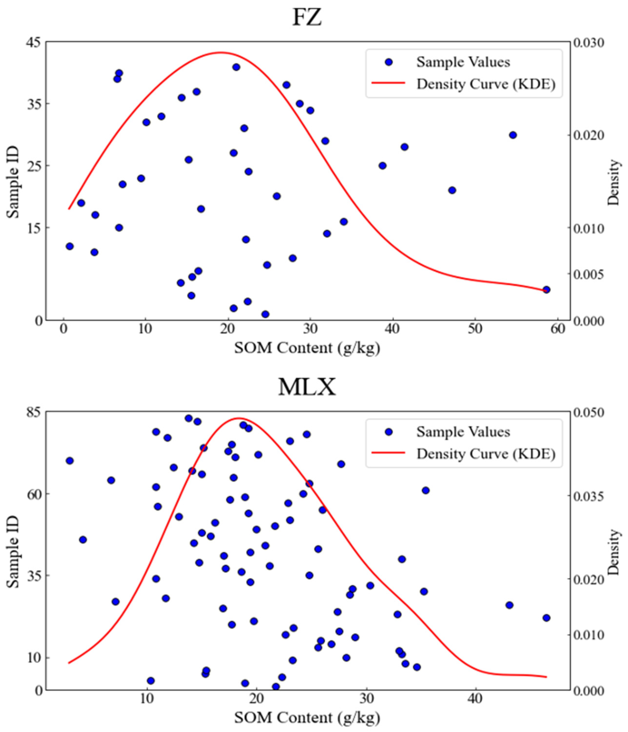
The analysis of the measured data (Figure 3) revealed significant spatial heterogeneity in soil organic matter (SOM) content across the study area. Specifically, the SOM content at the FZ sampling sites ranged from 0.75 to 58.63 g/kg, which is substantially higher than that at the MLX sites (2.94 to 46.41 g/kg).

In terms of distribution characteristics, the SOM content at the FZ sites exhibited a right-skewed distribution, primarily concentrated in the 15–25 g/kg range. A small number of low-value samples (<10 g/kg) and a few outliers with extremely high values (>40 g/kg) were also observed. This distribution pattern may be attributed to factors such as higher organic matter inputs in specific local areas, micro-environmental differences among sampling points, and a relatively limited sample size.

In contrast, the SOM content at the MLX sites showed an approximately normal distribution, with most values falling within the 15–25 g/kg range. The overall degree of variation was relatively small, indicating a more homogeneous pattern of organic matter accumulation in this region.

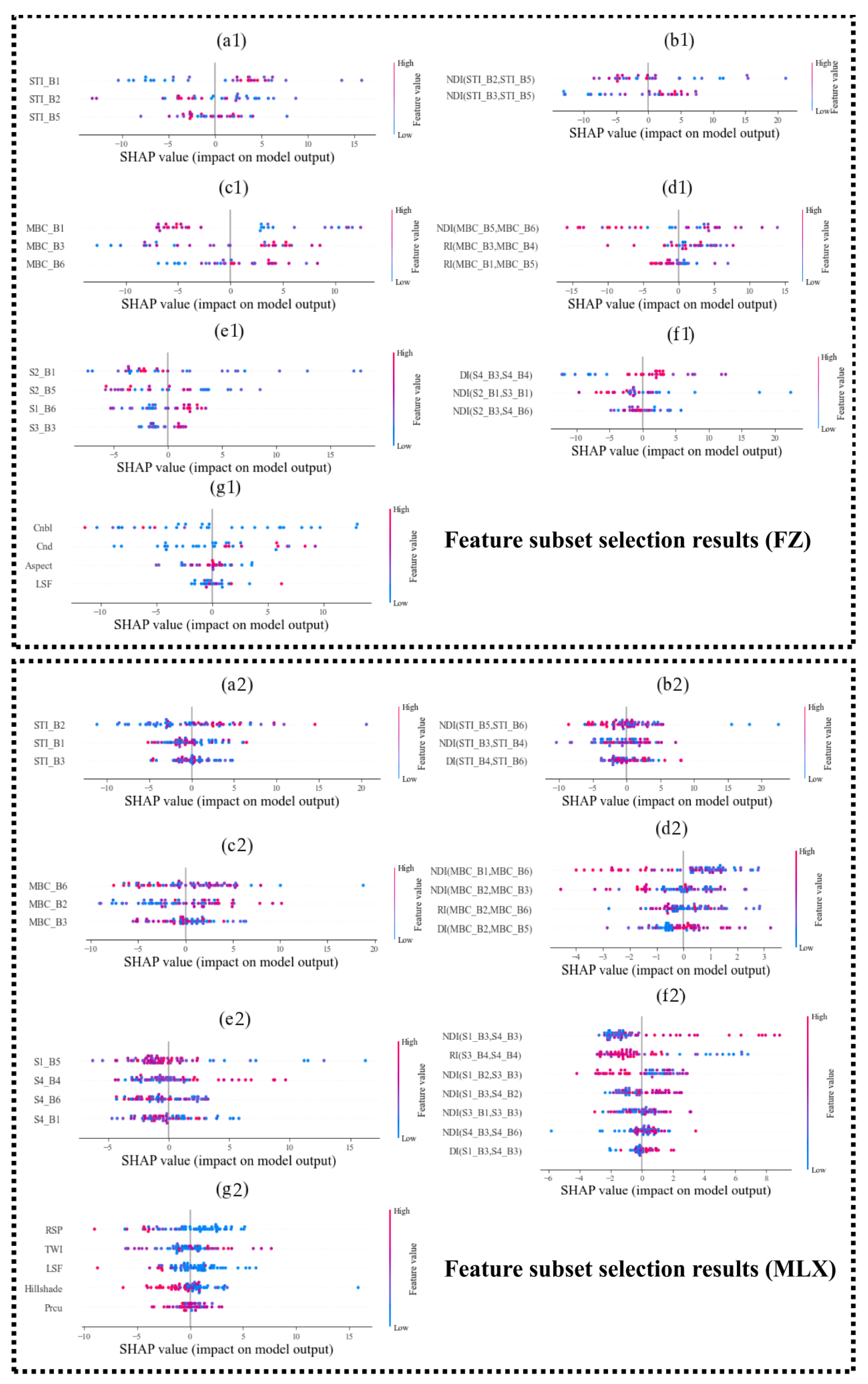
3.2. SOM Feature Variables

In this study, a multi-source feature dataset was constructed, including single-season imagery bands, single-season spectral indices, MABSC imagery bands, MABSC spectral indices, MFOC imagery bands, MFOC spectral indices, and topographic covariates. The FOI-XGB algorithm was used for feature selection, and SHAP values were employed to quantitatively assess the importance of each feature in SOM prediction.

According to the selection results (Figure 4), in the feature screening of single-season, MABSC, and MFOC imagery, bands B1 (blue), B2 (green), B3 (red), and B5/B6 (shortwave-infrared) were frequently selected. This aligns with previous studies on the sensitivity of these bands to soil iron oxides and SOM functional groups [53,54]. In particular, MABSC bands B3 and B6 showed high contributions in both study areas, which are closely related to mineral spectral characteristics and the interaction of organic matter and moisture under bare-soil conditions. B3 effectively indicated iron oxide content [55], and B6 responded stably to changes in soil moisture and humus content [56,57].

In MFOC feature selection, a seasonal pattern was observed in both regions. In the FZ area, bands from summer (S2_B1, S2_B5), autumn (S3_B3), and spring (S1_B6) were selected, along with seasonal combination indices such as the winter DI (S4_B3, S4_B4), summer–autumn NDI (S2_B1, S3_B1), and summer–winter NDI (S2_B3, S4_B6). In the MLX area, bands from spring (S1_B5) and winter (S4_B4, S4_B6, S4_B1) were primarily selected, alongside indices such as spring–winter NDI (S1_B3, S4_B3), autumn–winter RI (S3_B4, S4_B4), spring–autumn DI (S1_B2, S3_B3), spring–winter NDI (S1_B3, S4_B2), autumn DI (S3_B1, S3_B3), winter NDI (S4_B3, S4_B6), and spring–winter (S1_B3, S4_B3). These results indicate that spectral characteristics from spring, autumn, and winter were selected most frequently, suggesting a stronger indicative role in SOM prediction.

For the topographic covariates, factors such as Cnbl, Aspect, Cnd, and LSF were selected in the FZ area. These variables capture terrain complexity and mountain fluctuations over large areas and are closely related to the spatial heterogeneity of SOM, as SOM accumulation is influenced by hydrothermal conditions and vegetation uptake of organic matter. In the MLX area, selected factors included RSP, TWI, LSF, Hillshade, and Prcu. Here, the SOM in this area is primarily influenced by hydro-topographic processes and erosion–sedimentation dynamics.

3.3. SOM Mapping and Validation

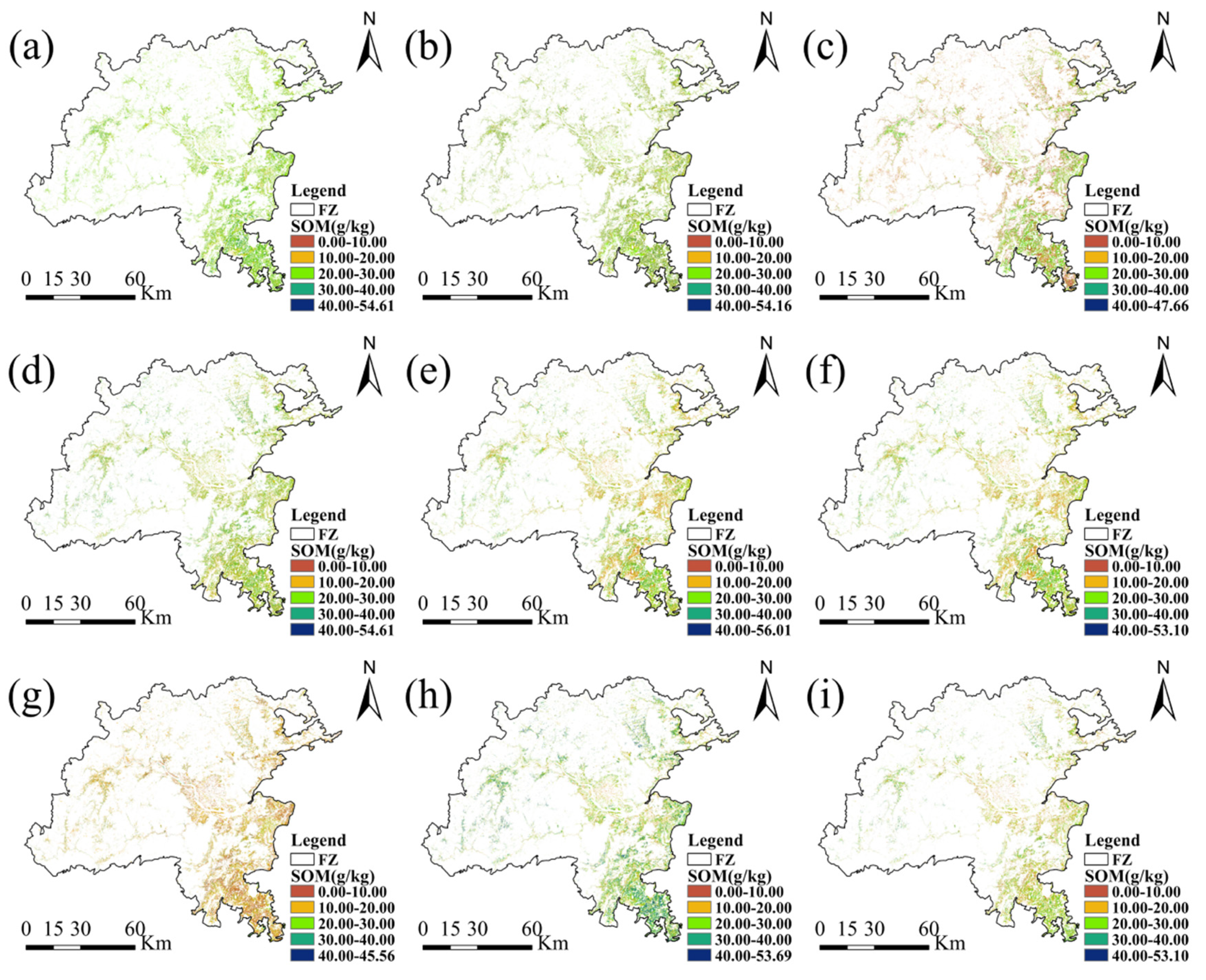
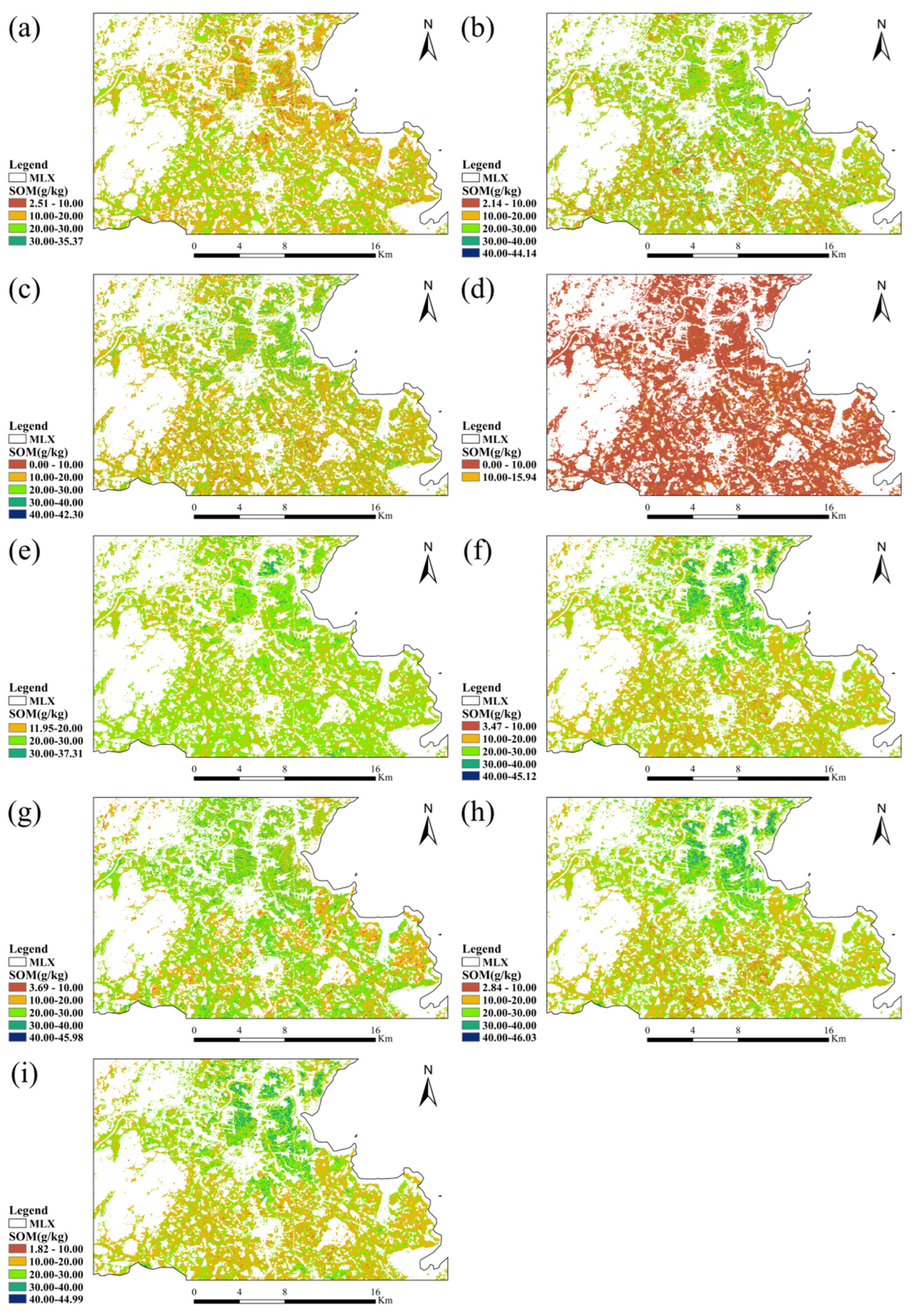
Based on the aforementioned feature selection results, nine different SOM feature combinations were designed in this study: single-temporal image bands (STI-Band), single-temporal vegetation indices (STI-Index), MABSC image bands (MABSC-Band), MABSC vegetation indices (MABSC-Index), MFOC image bands (MFOC-Band), MFOC vegetation indices (MFOC-Index), topographic covariates (TC), spectral combination modeling (MABSC-Band + MFOC-Index), and spectral–topographic combination modeling (MABSC-Band + MFOC-Index + TC). These combinations were used to assess and compare SOM prediction performance under different feature input conditions. Model evaluation was carried out using R², RMSE, and the ratio of RPD as evaluation metrics in order to quantify the contribution of multi-source features to SOM prediction accuracy (Figure 5 and Figure 6).

The results indicate that the “multi-temporal image fusion and FOI-XGB” framework for SOM mapping demonstrated the best prediction performance in both study areas (

Table 2. Modeling validation with multi-feature subsets.

	FZ			MLX
Modeling feature subsets	R2	PRD	RMSE	R2	PRD	RMSE
STI-Band	−0.37	0.95	12.56	0.11	1.08	7.2
STI-Index	0.01	1.1928	10.10	0.02	1.02	7.44
MABSC-Band	0.19	1.64	8.83	0.22	1.18	6.77
MABSC-Index	−0.23	1.00	11.88	0.09	1.12	2.93
MFOC-Band	−0.27	0.95	12.03	0.13	1.10	7.01
MFOC-Index	0.37	1.49	8.33	0.40	1.35	5.73
TC	0.25	1.22	9.48	0.18	1.14	6.80
MABSC-Band + MFOC-Index	0.44	1.63	8.04	0.42	1.41	5.54
MABSC-Band + MFOC-Index + TC	0.51	1.59	7.52	0.47	1.59	5.17

). The modeling approach based on multi-source data fusion achieved the best prediction performance in both regions. In the FZ area, the model yielded an R² of 0.51 (PRD = 1.59, RMSE = 7.52), while in the MLX area, the R² reached 0.47 (PRD = 1.59, RMSE = 5.17).

According to the results presented in Table 2, the MABSC-Band model performed relatively well in both the FZ (R² = 0.19, PRD = 1.64) and MLX (R² = 0.22, PRD = 1.18) regions. Compared to STI-Band, the spectral features extracted from MABSC showed better predictive performance, with R² improvements of 0.56 for FZ and 0.11 for MLX. This improvement may be attributed to the more direct response of raw spectral bands to soil physicochemical properties under bare-soil conditions.

Similarly, the spectral indices from MFOC exhibited stronger predictive capability. For FZ and MLX, the R² values reached 0.37 and 0.40, respectively—increases of 0.36 and 0.38 compared to the traditional single-temporal index (STI-Index). This suggests that temporal spectral indices may have greater advantages in capturing the dynamic variations of SOM. It is worth noting that models using only single-temporal imagery features (STI-Band and STI-Index) performed poorly overall. In fact, the R² for STI-Band in the FZ region was negative (−0.37), indicating that single-date remote sensing data may fail to effectively characterize the spatial variability of SOM in complex terrain areas.

Further analysis of feature combinations revealed that the synergistic use of MABSC-Band and MFOC-Index significantly improved model prediction accuracy, achieving R² values of 0.44 and 0.42 in the FZ and MLX regions, respectively. Upon incorporating topographic covariates, model performance reached its optimal level, with R² values increasing to 0.51 for FZ and 0.47 for MLX. Notably, topographic factors showed marked regional differences—their independent predictive capacity in the FZ region (R² = 0.24) was significantly higher than that in the MLX region (R² = 0.18). In terms of prediction accuracy, the best-performing combination models in both regions achieved PRD values above 1.5 (FZ = 1.59, MLX = 1.59), indicating a reliable prediction level. From the evaluation results of RMSE, the MMT model combination (MABSC-Band + MFOC-Index + TC) demonstrated the highest prediction accuracy, achieving the lowest RMSE values for both study areas (FZ = 7.52, MLX = 5.17). These results indicate that the multi-source feature fusion strategy significantly improved model performance. Furthermore, the analysis of PRD variations in feature subsets demonstrates that the spectral combination (MABSC-Band + MFOC-Index) contributed most significantly to performance improvement. The PRD reached 1.63 in FZ and increased from 1.18 and 1.35 to 1.41 in MLX. This confirmed the critical role of multi-temporal spectral indices in enhancing the model’s predictive capability.

From the perspective of spatial distribution, the SOM maps revealed clear differences between the two study areas. The FZ region exhibited high spatial heterogeneity with three prominent patterns: (1) a low-value zone corresponding to urban centers and surrounding areas influenced by urbanization, likely due to soil sealing and anthropogenic disturbance; (2) medium-to-high SOM concentrations in the eastern and southeastern coastal plains, reflecting long-term agricultural accumulation; and (3) high-SOM values in scattered farmland patches in western and northern mountainous areas, potentially related to microclimatic conditions and slower organic matter decomposition rates. This complex spatial pattern highlights the compound effects of diverse topography and human activities on SOM distribution in the FZ area. In contrast, the MLX region displayed a more distinct gradient pattern, with continuous high-SOM zones in the northern and western traditional farming areas—attributable to long-term rice cultivation—and low-SOM zones in the southeastern urban fringe and coastal areas, likely influenced by urban expansion and salinization. Compared to FZ, MLX exhibited more consistent and contiguous spatial patterns, largely due to two factors: smaller spatial extent enhancing spatial autocorrelation and a more homogeneous soil type and land management system reducing complexity. This contrast vividly demonstrates how spatial scale and land-use practices shape SOM spatial distribution.

3.4. FOI-XGB Model Performance Validation

The proposed FOI-XGB model integrates the efficient predictive capability of XGBoost, the interpretability of SHAP analysis, and the robust feature selection of RFECV, enabling the automated selection and physical interpretation of optimal predictors from a multi-source, high-dimensional feature space, including raw spectral bands, spectral indices, and topographic factors.

To further validate the effectiveness of the feature variables selected by FOI-XGB, it was compared against three other feature selection approaches: SHAP, the Pearson correlation coefficient (PCC), and a combined method (CorrSHAP) that integrates SHAP and PCC. Due to the excessive number of spectral index variables selected by the PCC method, the number of features was controlled by retaining only the top 10 variables with the highest absolute correlation coefficients. The CorrSHAP method employed a two-stage filtering strategy: it first eliminated irrelevant variables using SHAP, then conducted a secondary selection based on PCC values.

The performance of these three selection methods was compared with that of FOI-XGB, as shown in Figure 7.

By comparing the performance of different feature selection methods, this study found that the traditional PCC method (R² = 0.27 and 0.36) yielded lower predictive accuracy due to its reliance solely on linear correlations. The XGBoost + SHAP approach improved accuracy to R² = 0.36 and 0.42 by capturing nonlinear interactions among features, thus outperforming PCC in precision [53], but it still suffered from redundant features. The CorrSHAP method, which combines SHAP with PCC in a two-stage selection process, further improved performance to R² = 0.39 and 0.43. However, its effectiveness was limited by fixed thresholds and the linear nature of the secondary filtering.

In contrast, the FOI-XGB method proposed in this study adopts an innovative strategy of “SHAP-based pre-screening + RFECV dynamic optimization”, achieving significantly superior results in the FZ and MLX regions with R² values of 0.51 and 0.47, respectively. The corresponding RMSE values (7.52 and 5.17) and PRD values (1.59 and 1.59) also outperformed all benchmark methods.

These findings demonstrate that integrating SHAP with RFECV effectively overcomes the limitations of traditional approaches in capturing nonlinear relationships, removing redundant features, and reducing dependency on manual thresholds, thereby simultaneously enhancing both the accuracy and robustness of feature selection.

4. Discussion

4.1. Regional Adaptability of the FOI-XGB Model

The feature selection results for SOM inversion in the FZ and MLX study areas reveal both commonalities and region-specific differences in optimal band selection and spectral index construction. The findings show that MABSC bands can effectively capture spectral signals directly associated with exposed soils, while the MFOC and TCs are more suitable for reflecting seasonal variations and topographic characteristics unique to each region. These results not only demonstrate regional differentiation patterns but also provide a practical reference for remote sensing modeling of soil properties in other areas.

In terms of common features, bands B3, B5, and B6 appeared with high frequency across all three spectral feature selection strategies. Notably, bands B3 and B6 showed consistently strong contributions in MABSC, confirming their sensitivity to key soil characteristics: B3 to iron oxides and B6 to interactions between soil organic matter and moisture.

Region-specific differences were also significant. The MFOC results revealed that FZ exhibited a preference for summer–winter band combinations, while MLX showed a stronger affinity for spring–autumn–winter combinations. Regarding topographic covariates, FZ predominantly selected variables associated with terrain ruggedness, whereas MLX favored parameters indicative of hydrological processes.

These differences likely stem from distinct regional climate conditions and soil characteristics. FZ, a typical hilly red soil region, features soils rich in iron oxides and is significantly affected by terrain variability. These factors explain the region’s preference for summer and winter bands, as the strong weathering in hot, rainy summers and the exposure during dry winters yield distinctive spectral features useful for SOM estimation. The emphasis on terrain-related covariates (e.g., Cnbl, Aspect) is also consistent with the area’s complex topography.

In contrast, MLX, a coastal plain characterized by paddy soils, is more influenced by agricultural practices and surface hydrology. The accumulation of water in low-lying areas promotes the decomposition of organic matter [58,59]. Summer coincides with the anaerobic flooding phase in rice cultivation systems, making spring, autumn, and winter bands more effective in capturing changes in soil conditions throughout the rice-growing cycle. Moreover, MLX is situated at the downstream estuary of the Mulan River watershed, where it is significantly influenced by hydrological dynamics and alluvial erosion processes. This explains the predominant selection of such topographic covariates in this area.

The feature selection patterns identified in this study provide important practical insights. While regional differences exist, bands such as B3 and B6 demonstrate robust performance across both study areas, offering a solid baseline for applications in other regions. At the same time, the findings underscore the importance of adapting feature selection strategies to local environmental conditions: mountainous and hilly regions should focus on terrain variation and seasonal shifts in moisture, whereas agricultural plains require attention to water dynamics and cropping cycles. These results not only explain the observed regional differences but also offer theoretical and methodological guidance for extending SOM remote sensing applications to other ecological zones. Future applications of the FOI-XGB model should consider both the foundational role of key spectral bands and the need for context-specific adjustments based on local climate, soil type, and land-use patterns to ensure accurate and reliable inversion outcomes.

4.2. Technical Framework for SOM Remote Sensing Mapping

This study constructed an integrated model by combining bare-soil bands extracted through MABSC, multi-temporal indices optimized via MFOC, and topographic covariates selected using FOI-XGB. The model demonstrated optimal performance in both study areas. According to the modeling results (Table 2), the FZ region achieved an R² of 0.51, an RMSE of 7.52, and an RPD of 1.59; the MLX region achieved an R² of 0.47, an RMSE of 5.17, and an RPD of 1.59. The RPD values in both regions exceeded the practical prediction threshold of 1.5, indicating a significant advantage of this approach over models relying on single-date imagery or unoptimized features.

The results also revealed notable regional differences: the independent predictive power of topographic factors in the FZ region (RPD = 1.22) was clearly higher than that in the MLX region (RPD = 1.14), confirming the adaptability of the proposed method. It is worth noting that although the MLX region had a larger sample size (83 samples) than the FZ region (41 samples), its smaller spatial extent and more uniform soil characteristics provided more favorable conditions for model training, which may explain the greater stability of its modeling results.

A comparative analysis with domestic and international studies highlights the superior inversion performance of this framework in subtropical mountainous and hilly areas. Compared with previous studies—such as those using bare-soil synthesis in plateau agricultural areas (R² = 0.26) [42], multi-temporal composites in plain regions (R² = 0.56) [60], and time-series imagery combined with topographic covariates in southeastern hilly areas (R² = 0.31) [24]—the proposed model maintains better performance (R² = 0.47–0.51, PRD = 1.59), even under the more complex terrain conditions of mountainous hills and the stringent evaluation of tenfold cross-validation. These results demonstrate that the proposed multi-source feature fusion approach has greater adaptability and stability under complex terrain conditions.

From a data source perspective, the Landsat satellite series offers reliable support for SOM inversion due to its stable coverage and free availability [19], enabling consistent extraction of bare-soil information and the construction of environmental variable combinations. However, despite the strong performance of this framework, several limitations remain:

(1) A smoothing effect was observed, where the predicted standard deviations were lower than those of the measured samples, potentially underestimating low values in FZ or compressing high values in MLX.

(2) Insufficient sample size and variability in SOM measurement methods in the FZ region may have introduced errors.

(3) In applications across large-scale, complex terrains with limited samples, the lack of spatial representativeness could reduce prediction stability. Moreover, since this study primarily focused on hilly and paddy soil environments, its applicability in large plains, arid zones, or cold regions still requires further verification.

4.3. Limitations and Future Perspectives

Although the proposed multi-temporal image fusion + TC + FOI-XGB framework demonstrated high accuracy and regional adaptability for SOM prediction in subtropical coastal mountainous regions, several limitations remain and merit further discussion.

First, a smoothing effect was observed in the predicted results, where the standard deviations of the predicted SOM values were consistently lower than those of the measured data. This may have led to the underestimation of low-SOM values in the FZ region and the compression of high-SOM values in the MLX region. Such phenomena have been frequently reported in soil prediction studies, especially in heterogeneous terrains [61].

Second, the limited sample size in the FZ region (n = 41) and the inconsistency in SOM measurement methods—potassium dichromate oxidation in FZ versus elemental analysis in MLX—may have introduced systematic errors and reduced model reliability. Moreover, while a SOC-to-SOM conversion factor of 1.724 was applied, studies have questioned its universal applicability across soil types, land-use systems, and climatic conditions [39,62]. Future research should consider developing region-specific empirical conversion models or directly conducting SOC research to reduce uncertainties related to conversions.

In addition, in large-scale, topographically complex regions, limited and sparsely distributed samples may not fully capture spatial variability, thereby affecting model generalizability and spatial representativeness. In such cases, spatial heterogeneity may exceed the ability of current models to resolve local patterns, particularly when relying on single-date or low-density sample observations [63].

To address these limitations, future research is encouraged to focus on the following directions: constructing large-scale, multi-temporal, standardized soil databases to enhance training diversity and consistency; implementing stratified spatial sampling or terrain-based zoning strategies to improve representativeness; developing localized SOC-to-SOM conversion relationships or building direct SOC models; integrating multi-source remote sensing to better capture complex surface variability; and establishing cross-regional transfer learning frameworks for enhanced model generalization.

5. Conclusions

This study developed a regional-scale SOM inversion framework tailored to subtropical coastal mountainous areas by integrating multi-temporal Landsat imagery, intelligent high-dimensional feature selection, and machine learning modeling. The main conclusions are as follows:

1. The FOI-XGB model enables efficient, interpretable, and automated feature selection.

The proposed FOI-XGB model, which integrates the predictive power of XGBoost, the interpretability of SHAP, and the recursive elimination capability of RFECV, enabled the automatic identification of optimal feature subsets without manual specification. Compared with traditional methods such as PCC (R² = 0.27/0.36) and SHAP (R² = 0.36/0.42), the FOI-XGB model achieved the highest prediction accuracy in both Fuzhou (FZ) and Mulanxi (MLX), with R² values of 0.51 and 0.47, respectively. The corresponding PRD values reached 1.59 in both regions, and the RMSE values were 7.52 g/kg (FZ) and 5.17 g/kg (MLX), outperforming the CorrSHAP approach (R² = 0.39/0.43) in terms of accuracy, robustness, and generalizability.

2. Multi-temporal compositing significantly improves model accuracy and stability.

The MABSC method effectively removed vegetation interference and extracted bare-soil reflectance features, while the MFOC method identified seasonal spectral indicators sensitive to SOM variation. In FZ and MLX, MABSC improved the R² values by 0.56 and 0.11, respectively, while MFOC increased the R² values by 0.36 and 0.38. Their combination further enhanced model accuracy to R² = 0.44 (FZ) and R² = 0.42 (MLX), demonstrating substantial advantages over single-date models (e.g., STI-Band, R² = −0.37 in FZ) and confirming the importance of temporal information for SOM inversion.

3. The integrated framework exhibits strong generalization and cross-regional adaptability.

The full framework—combining MABSC, MFOC, topographic covariates, and FOI-XGB—achieved high inversion performance across different spatial and environmental contexts. In both study areas, the model consistently reached R² > 0.47, PRD = 1.59, and RMSE < 8 g/kg. The improvement in R² over single-source models exceeded 60%. The framework performed robustly despite differences in sample size (41 in FZ vs. 83 in MLX), spatial extent (FZ: 11,597 km²; MLX: 538 km²), and landform types, confirming its scalability and transferability for SOM mapping in other complex terrains.