Remote Sensing-Based Analysis of the Coupled Impacts of Climate and Land Use Changes on Future Ecosystem Resilience: A Case Study of the Beijing–Tianjin–Hebei Region

Abstract

Urban and regional ecosystems are increasingly challenged by the compounded effects of climate change and intensive land use. In this study, a predictive assessment framework for ecosystem resilience in the Beijing–Tianjin–Hebei region was developed by integrating multi-source remote sensing data, with the aim of quantitatively evaluating the coupled effects of climate change and land use change on future ecosystem resilience. In the first stage of the study, the SD-PLUS coupled modeling framework was employed to simulate land use patterns for the years 2030 and 2060 under three representative combinations of Shared Socioeconomic Pathways and Representative Concentration Pathways (SSP1-2.6, SSP2-4.5, and SSP5-8.5). Building upon these simulations, ecosystem resilience was comprehensively evaluated and predicted on the basis of three key attributes: resistance, adaptability, and recovery. This enabled a quantitative investigation of the spatio-temporal dynamics of ecosystem resilience under each scenario. The results reveal the following: (1) Temporally, ecosystem resilience exhibited a staged pattern of change. From 2020 to 2030, an increasing trend was observed only under the SSP1-2.6 scenario, whereas, from 2030 to 2060, resilience generally increased in all scenarios. (2) In terms of scenario comparison, ecosystem resilience typically followed a gradient pattern of SSP1-2.6 > SSP2-4.5 > SSP5-8.5. However, in 2060, a notable reversal occurred, with the highest resilience recorded under the SSP5-8.5 scenario. (3) Spatially, areas with high ecosystem resilience were primarily distributed in mountainous regions, while the southeastern plains and coastal zones consistently exhibited lower resilience levels. The results indicate that climate and land use changes jointly influence ecosystem resilience. Rainfall and temperature, as key climate drivers, not only affect land use dynamics but also play a crucial role in regulating ecosystem services and ecological processes. Under extreme scenarios such as SSP5-8.5, these factors may trigger nonlinear responses in ecosystem resilience. Meanwhile, land use restructuring further shapes resilience patterns by altering landscape configurations and recovery mechanisms. Our findings highlight the role of climate and land use in reshaping ecological structure, function, and services. This study offers scientific support for assessing and managing regional ecosystem resilience and informs adaptive urban governance in the face of future climate and land use uncertainty, promotes the sustainable development of ecosystems, and expands the applicability of remote sensing in dynamic ecological monitoring and predictive analysis.

1. Introduction

The concept of ‘ecosystem resilience’ is defined as the capacity of an ecosystem to sustain its function when faced with disturbances [1,2,3]. It serves as a key indicator of ecological health, playing a vital role in preserving ecosystem services and sustaining the regional ecological balance. However, the rapid growth in socioeconomic development and urbanization is placing escalating pressure on the maintenance of ecosystem resilience [4,5,6]. The intensifying impacts of extreme weather events, habitat loss, declining biodiversity, and the weakening of ecosystem services worldwide indicate that ecosystem resilience is at risk [7,8]. Therefore, many scholars are dedicated to researching ways to improve and reverse this situation [7,9,10,11,12]. The key to advancing research in this area is to explore the primary driving mechanisms behind changes in ecosystem resilience.

Land use change serves as a primary factor influencing ecosystem resilience. With the advancement of urbanization and industrialization, the growing concentration of populations and industries in cities is heightening the demand for construction land. As a result, cultivated land, forestland, grassland, and natural ecosystems are being progressively displaced, leading to a reduction in ecological space. These alterations, in turn, disrupt the provision of ecosystem services and functions [9], modify the landscape structure and composition, and ultimately affect fundamental ecosystem processes [13,14]. These impacts collectively shape the dynamics of ecosystem resilience, highlighting the critical role of land use in its transformation [15]. Initially, many scholars focused on evaluating the historical and current state or value of ecosystem resilience [9,16,17]. For instance, Jie et al. analyzed changes in ecosystem resilience in the Taohe River Basin, China, from 2000 to 2020, utilizing historical land cover data [9]. Duo et al. explored the ecosystem dynamics of Nanchang, China, using 2005–2020 land use data and therefore clarified the historical trend of ecosystem resilience and its influencing mechanism [18]. Recently, some scholars have shifted their focus toward evaluating and investigating the possible effects of future land use change on ecosystem resilience. For example, Wan et al. predicted coastal ecosystem resilience utilizing future (2030) land use data generated by the Patch Generation Land Use Simulation (PLUS) model [19,20], and Xia et al. predicted the ecosystem resilience dynamics in Hangzhou, China, for the year 2035 based on land use data produced by the Future Land Use Simulation (FLUS) model [21]. Although these studies have extensively explored the relationships between land use change and ecosystem resilience, they have largely overlooked the growing impact of future climate change on ecosystem resilience.

Notably, the intensification of climate change will also have a significant impact on ecosystem resilience. Climate change intensification introduces significant uncertainty into ecosystem stability and adaptive capacity and influences ecosystem resilience through multiple interconnected mechanisms [22]. It reduces biodiversity, diminishing functional redundancy and adaptive capacity. Changes in temperature and precipitation alter ecosystem structures, disrupting species composition and habitat stability [23]. Essential ecological processes, such as nutrient cycling and the hydrological balance, are disturbed, further destabilizing ecosystems. Additionally, the rising occurrence and severity of extreme weather events cause sudden ecological disruptions, while habitat fragmentation isolates populations, limiting migration and genetic diversity [24]. These changes weaken the ecosystem’s self-regulation and recovery mechanisms, increasing its vulnerability to long-term environmental shifts and ultimately leading to a decline in ecosystem resilience [25]. Therefore, existing studies that focus solely on the impact of land use dynamics on ecosystem resilience have clear limitations. There is an urgent need to systematically explore the impact mechanisms from the coupled perspective of climate change and land use change.

The coupled effects of land use and climate change on ecosystem resilience can be comprehensively assessed by incorporating the SSP-RCP scenarios for multi-scenario simulations. The SSP-RCP scenarios—which integrate Shared Socioeconomic Pathways (SSPs) and Representative Concentration Pathways (RCPs), as established by the Coupled Model Intercomparison Project Phase Six (CMIP6) [26]—provide a robust scientific framework for exploring the coupled effects of land use and climate change on ecosystem resilience [27]. By incorporating socioeconomic development trajectories alongside greenhouse gas concentration pathways, this framework enables a more comprehensive assessment of future climate change impacts [28]. In recent years, researchers have integrated land use simulation models with SSP-RCP climate change scenarios to project future land use. For example, Wang et al. employed the Conversion of Land Use and its Effects at Small Region Extent (CLUE-S) model and the PLUS model to simulate and predict land use structure in Bortala, China, under different SSP-RCP climate change scenarios for the year 2050 [29]. Yang et al. utilized the Cellular Automata (CA)–Markov model to simulate and predict land use dynamics in the Chao Phraya Basin, Thailand [30]. Li et al. applied a system dynamics (SD) model and PLUS model to simulate future land use patterns under different SSP-RCP scenarios in Wuhan, China [31]. Among these models, the combination of SD and PLUS models (SD-PLUS) has demonstrated high accuracy in predicting the quantity as well as the spatial distribution of land use types [32], highlighting their excellent simulation and prediction prospects. The integration of these land use simulation models with SSP-RCP scenarios offers new possibilities for exploring the coupled influences of land use and climate change on future ecosystem resilience.

Considering that the coupled effects of land use and climate change on ecosystem resilience remain unclear, the Beijing–Tianjin–Hebei (BTH) region was selected as the research zone in this study, with 2030 and 2060 as key time nodes. The simulation horizon spans from 2030 to 2060 to align with China’s nationally determined ‘dual carbon’ goals—emission peaking by 2030 and carbon neutrality by 2060—thereby ensuring that the projected ecological resilience trends are contextually relevant to the region’s future policy trajectory. By integrating SSP-RCP scenarios with the SD-PLUS model, a new assessment and prediction framework was developed for evaluating ecosystem resilience. The objectives of this study are (1) to simulate the spatial distribution of land use under SSP-RCP scenarios for the key time nodes of 2030 and 2060 in the BTH region, (2) to predict future ecosystem resilience in the BTH region under different SSP-RCP scenarios, (3) to investigate the differentiated impacts of coupled climate and land use change scenarios on ecosystem resilience, and (4) to propose an ecological management zoning plan for the BTH region and offer targeted insight into ecological governance for each zone. This study not only provides a scientific basis for formulating synergistic policies on climate adaptation and land management to promote sustainable urban development but also broadens the practical scope of remote sensing applications in resilience assessment and long-term ecosystem monitoring.

2. Materials and Methods

2.1. Study Area

The BTH region (35°03′N–42°40′N, 113°27′E–119°50′E), serving as the political center of China with Beijing and Tianjin as core cities, significantly influences economic activity in Hebei Province (Figure 1b). Bordered by the Bohai Sea to the east, the region’s landscape transitions from northwest to southeast, encompassing the Taihang and Yanshan mountainous areas, and covers diverse landscapes, ranging from the coast, plain, inland plateaus, and mountains. Additionally, the study area encompasses three major ecological functional conservation districts: the Bashang Plateau Ecological Protection Zone, the Yanshan Mountain Water Conservation and Soil Retention Zone, and the Taihang Mountain Water Conservation and Soil Retention Zone (Figure 1c).

Since the implementation of the reform and opening-up policies and the Beijing–Tianjin–Hebei coordinated development strategy, the BTH region has become one of China’s most important economic zones. By 2024, the gross domestic product (GDP) of the region had reached CNY 11.5 trillion, 2.1 times that in 2013. It is now the most densely populated, most urbanized, and fastest-growing urban agglomeration in northern China in terms of socioeconomic development. However, the rapid development of society and the economy, along with human activities, continues to affect ecological spaces, leading to local ecosystem deterioration and environmental vulnerability, all of which are weakening the region’s ecosystem resilience and posing threats to future development and long-term sustainability.

2.2. Data Sources

The data in this study were compiled from multi-source remote sensing datasets and open-access environmental and socioeconomic platforms (

Table 1. Major data sources.

Classification	Data Name	Data Sources	Resolution Ratio
Land use data	Land use data (2005–2020, at five-year intervals)	Chinese Academy of Sciences Resource and Environmental Science Data Center (https://www.resdc.cn/)	30 m
Natural environmental data	Elevation data (DEM)	Geospatial Data Cloud (https://www.gscloud.cn/)	30 m
	Precipitation	Space-time three-pole environmental big data platform (https://portal.casearth.cn/poles)	1000 m
	Temperature
	Potential transpiration	National Tibetan Plateau Data Center (https://data.tpdc.ac.cn/)	100 m
	Available moisture content of vegetation	HWSD soil database	100 m
	Vegetation root depth	HWSD soil database	100 m
	Precipitation erosivity	Calculated based on precipitation data	1000 m
	FVC	National Tibetan Plateau Data Center (https://data.tpdc.ac.cn/)	250 m
Socioeconomic data	Population	Data center for resources and environmental sciences of the Chinese Academy of Sciences (https://www.resdc.cn/)	100 m
	GDP		100 m
	Night-time lighting data	Earth Observation Group (https://payneinstitute.mines.edu/eog/, accessed on 28 October 2024)	500 m
	Primary road	National Geographic Information Resources Directory Service System (https://www.webmap.cn/)	100 m
	Railway
	Government location
	Water area
	Socioeconomic statistical data	CEI data (https://ceidata.cei.cn/) Statistical Yearbook of Beijing (https://tjj.beijing.gov.cn/) Statistical Yearbook of Tianjin (https://stats.tj.gov.cn/tjsj_52032/tjnj/) Yearbook of Hebei (http://tjj.hebei.gov.cn/)	/
SSP-RCP scenario setting data	Future precipitation	WorldClim Global Climate Data https://worldclim.org/	1000 m
	Future temperature
	Future GDP	China Climate Change Info-Net (https://www.climatechange.cn/)	5000 m
	Future urbanization ratio
	Future population

). Remotely sensed variables include land use/cover (2000–2020), the digital elevation model (DEM), annual precipitation and temperature, the NDVI, and fractional vegetation cover (FVC) derived from satellite-based observations. Socioeconomic variables such as the population, urbanization rate, GDP, night-time lights, infrastructure distribution, and fixed-asset investment were obtained from national statistical databases and geospatial vector datasets (e.g., railways and government locations).

Future climate and population projections under the SSP1-2.6, SSP2-4.5, and SSP5-8.5 scenarios were derived from CMIP6 simulations (e.g., BCC-CSM2-MR), and satellite- and ground-based observations were incorporated for model calibration.

All spatial data layers were resampled to a unified resolution of 100 m × 100 m to ensure consistency in spatial analysis. Nearest-neighbor resampling was applied for categorical data such as land use/cover, while bilinear interpolation was used for continuous variables, including the DEM, temperature, precipitation, GDP, population, and night-time lights.

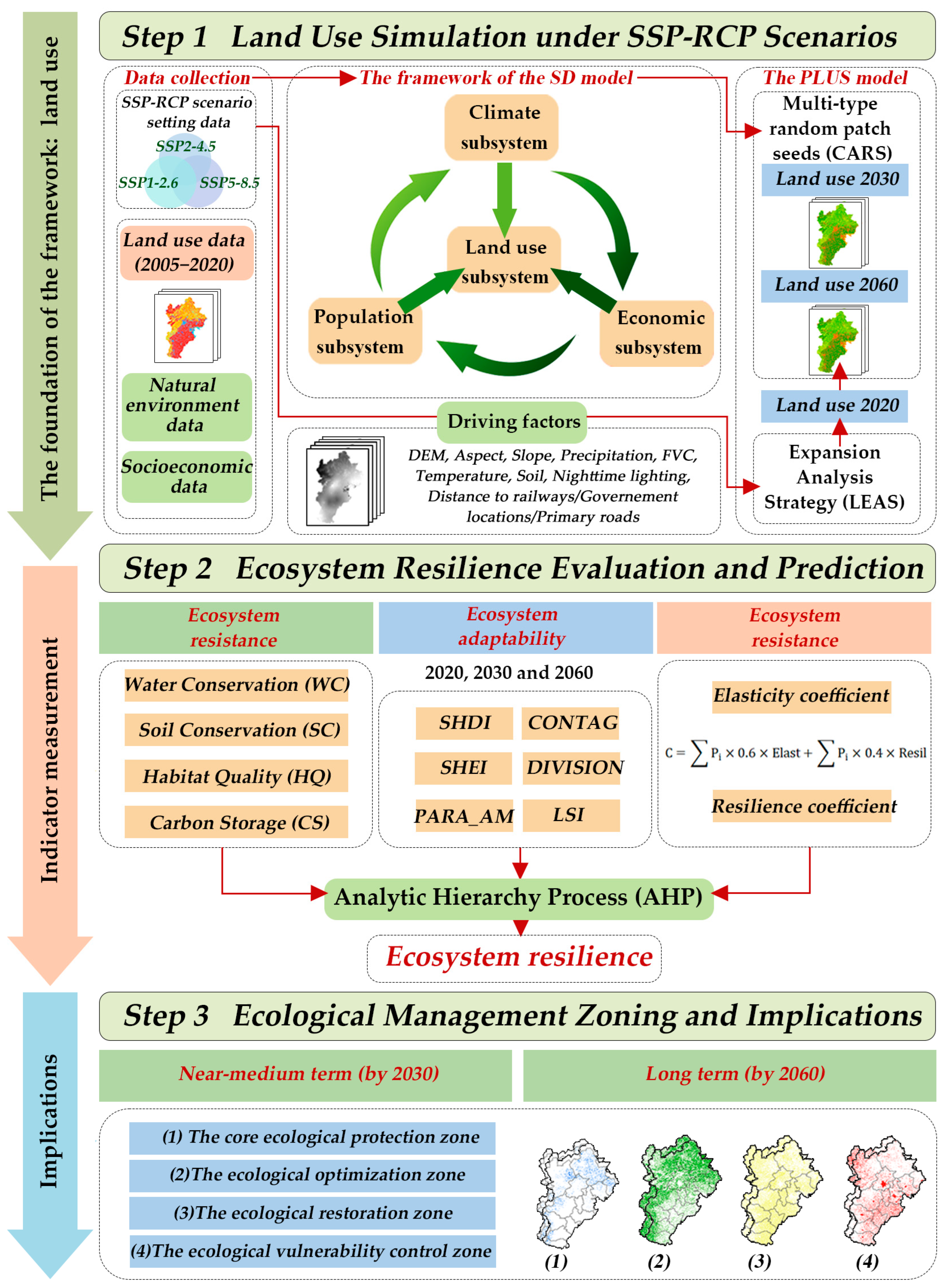
2.3. Research Framework

This study presents an assessment and prediction framework that integrates three SSP-RCP scenarios and the SD-PLUS model, as well as the InVEST and Fragstats models (Figure 2). Using this framework, we analyzed the future dynamics of the BTH region under the combined effects of land use and climate change for the years 2020, 2030, and 2060 in the SSP1-2.6, SSP2-4.5, and SSP5-8.5 scenarios. Based on our findings, we propose an ecological management zoning plan. The framework consists of three main components: (1) land use simulation and prediction for the BTH region in 2020, 2030, and 2060 under different SSP-RCP scenarios based on the SD-PLUS model; (2) quantitative assessment and prediction of three key attributes (resistance, adaptability, and recovery) of ecosystem resilience using the InVEST model and Fragstats, followed by an AHP weighted analysis to predict future ecosystem resilience dynamics; and (3) the development of an ecological management zoning plan using the natural breakpoint method based on the magnitude of ecosystem resilience changes.

2.4. Prediction of Future LUCC Demand in Different Scenarios Based on the SD-PLUS Coupled Model

2.4.1. Scenario Setting

To comprehensively explore the coupled influences of land use and climate change on ecosystem resilience, a multi-scenario approach was employed, considering various potential future conditions relevant to global ecological governance and regional socioeconomic development in the BTH region. Three typical SSP-RCP scenarios were selected in our study: SSP1-2.6, SSP2-4.5, and SSP5-8.5.

The SSP1-2.6 scenario synthesizes the SSP1 (sustainable development) socioeconomic pathway and the RCP2.6 (low emissions) climate pathway. This scenario emphasizes a balanced approach to economic growth and ecological sustainability. It envisions a future with improved living standards achieved through an economic transformation that prioritizes environmental protection, ensures food security, and enhances environmental quality [33]. This pathway promotes low-carbon land use and sustainable land management [34].

Combining SSP2 (moderate trends) and RCP4.5 (moderate emissions), the SSP2-4.5 scenario assumes that future trends will largely follow historical patterns, with moderate societal vulnerability and greenhouse gas forcing [35]. It represents a balanced socioeconomic development trajectory with moderate emissions and environmental change [36].

The SSP5-8.5 scenario couples SSP5 (rapid economic growth) with RCP8.5 (high emissions), depicting a future of rapid, unregulated economic expansion driven by fossil fuels and limited environmental concern. It anticipates significant urban sprawl, substantial climate change impacts (increased temperature, precipitation, frequency of extreme weather), and unconstrained land use conversion with minimal ecological protection [37].

These scenarios were selected to represent a series of plausible futures for the BTH region, enabling the prediction of future land use structure and ecosystem resilience amid diverse socioeconomic and climate circumstances.

2.4.2. SD Model for Land Use Structure Prediction

A system dynamics (SD) model was used to predict land use demand by integrating natural environmental, socioeconomic, and policy factors (Figure 3). This approach effectively captures the complex, ever-evolving, dynamic, and interconnected nature of land use change processes. The model framework, developed using Vensim software (v7.3.5), consists of four interconnected subsystems:

(1)

The Economic Subsystem

The economic subsystem incorporates variables such as GDP, the GDP growth rate, and fixed investment, reflecting the influence of economic development, particularly urbanization and infrastructure expansion, on construction land demand. Economic development is considered to play a vital role in the management of natural resources, with its most pronounced impact being the burgeoning of construction land, driven by the rising demand for urbanization and infrastructure development.

(2)

The Population Subsystem

The population subsystem encompasses variables such as the population growth rate, the urbanization rate, and food demand, representing the impact of population size and consumption patterns on land use structure.

(3)

The Climate Subsystem

The climate subsystem considers temperature and precipitation to be key climatic variables influencing water bodies and vegetation dynamics within forest and grassland ecosystems.

(4)

The Land Use Subsystem

The land use subsystem is considered the core part. Investment in the primary industry, along with factors such as precipitation, temperature, per capita food demand, and land policies, collectively shape the demand for cultivated land. Construction land demand is linked to population, GDP, and fixed-asset investment. Demands for other land types (forest, grassland, and water) are similarly driven by relevant factors and policies, with unused land acting as a balancing stock to maintain the total land area.

The system dynamics (SD) model was parameterized and validated using historical data from 2005 to 2020, which were obtained from national and regional statistical yearbooks, the China Economic Information (CEI) platform, and the China Urban Statistical Yearbook. Scenario-based projections from the SSP-RCP framework for the period from 2021 to 2060 were employed to simulate future trajectories. Linear regression equations describing inter-variable relationships were established using SPSS (Version 26.0), and the model structure was validated through dimensional consistency and equation tests in Vensim.

To incorporate the SSP-RCP scenarios into the SD model, key macro drivers, such as the GDP growth rate, urbanization rate, and population change, under SSP1-2.6, SSP2-4.5, and SSP5-8.5, were directly derived from WorldClim and the publicly available SSP database of CMIP6. These projections were used to drive changes in economic development, construction land expansion, and associated land demand modules within the SD structure. Climate-related variables, including projected temperature and precipitation under the SSP-RCP scenarios, were integrated as external forcing factors influencing cultivated land, grassland, forestland, and water area demand and ecological land pressure. For instance, precipitation trends were linked to water resource availability parameters, which in turn affected irrigation needs and cultivated land dynamics. Similarly, long-term temperature increases were factored into constraints on vegetation suitability and ecological land transitions.

2.4.3. PLUS Model for Land Use Spatial Distribution Prediction

The PLUS model, developed in [19], was used to spatially simulate future land use patterns. The model incorporates a CA model with the Land Expansion Analysis Strategy (LEAS) that relies on multi-type random patch seeds (CARS). This approach outshines other CA models in terms of enhancing simulation precision and generating more lifelike landscape patterns [38]. In previous studies, the PLUS model has demonstrated strong applicability and simulation accuracy in long-term land use projections, thereby providing a solid methodological foundation for the extended time horizon adopted in this study [35,37,39].

For the LEAS component, a total of 13 driving factors were selected, encompassing both natural and socioeconomic dimensions. Natural environmental factors included the digital elevation model (DEM), slope, aspect, temperature, precipitation, soil type, and fractional vegetation cover (FVC). Socioeconomic drivers comprised gross domestic product (GDP), population, county government locations, railways, primary roads, and night-time lights (a detailed justification for the inclusion of each variable is provided in Appendix A.1). All driver datasets were preprocessed in ArcGIS 10.3 to ensure that the coordinate system, spatial resolution, and format were consistent with the land use data. Euclidean distance rasters were calculated for all proximity-based factors.

The CARS parameter settings were optimized through iterative testing until the highest Kappa coefficient and Figure of Merit (FoM) values were obtained (detailed in Section 3.1.1). A patch generation threshold of 0.2 was found to yield the optimal results. Default values were used for the expansion coefficient (0.1) and seed percentage (0.1). The neighborhood size was set to 3, and the thread count to 16, in line with previous studies [40,41,42].

2.5. Ecosystem Resilience Evaluation Framework

Assessing resilience is challenging due to the complexity and dynamic nature of ecosystems, the wide variation in responses to disturbances across different scales and timeframes, and the limited understanding of many underlying mechanisms. However, this challenge can be addressed by using fundamental attributes or aspects of ecosystems as proxies for resilience. This study, therefore, evaluated ecosystem resilience using a framework based on three key attributes—adaptability, resistance, and recovery—reflecting the temporal process of the ecosystem’s response to disturbances [9]. The term ‘resistance’ refers to an ecosystem’s ability to withstand and adapt to environmental changes. Meanwhile, ‘adaptability’ describes its capacity to resist regime shifts and maintain functionality, often through internal restructuring [43,44], and the concept of ‘recovery’ signifies the ecosystem’s ability to return to its original state after experiencing disturbances [45].

2.5.1. Ecosystem Resistance

Ecosystem resistance, the ability to withstand disturbances, was evaluated based on key ecosystem service functions in the BTH region: water conservation (WC), soil conservation (SC), habitat quality (HQ), and carbon storage (CS), calculated with the Integrated Valuation of Ecosystem Services and Tradeoffs (InVEST) model [46].

To assess the impact of coupled climate and land use change, SSP-RCP scenario-specific climate projections of precipitation and temperature were incorporated either directly into InVEST modules or indirectly through their influence on land use transitions simulated using the SD-PLUS framework. The integration pathways are detailed below for each resistance component.

(1)

Water Conservation (WC)

WC was computed through the Annual Water Yield module of InVEST, which employs land use and average annual precipitation data, leveraging the Budyko curve approach [47] to estimate pixel-level annual water runoff. These estimates are then aggregated to determine the total water yield across the watershed. Essentially, the model provides a simplified representation of the hydrological cycle, emphasizing key processes such as precipitation, transpiration, and evaporation. For future scenarios, annual precipitation values were adjusted based on SSP-RCP climate projections to reflect differences among 2020, 2030, and 2060 conditions. Temperature-influenced evapotranspiration parameters were also adapted accordingly, enabling a climate-sensitive estimation of hydrological processes [48].

(2)

Soil Conservation (SC)

The Sediment Delivery Ratio (SDR) of the InVEST model is commonly employed to quantify the overland sediment yield and its delivery to stream networks in order to assess the SC capacity [49]. The SDR model uses rainfall erosivity (R factor) as a key input, which was recalculated for future periods based on SSP-RCP precipitation trends to account for changing rainfall intensity and erosion potential. This enables a more realistic assessment of soil retention under future climate variability [50].

(3)

Habitat Quality (HQ)

The Habitat Quality module is designed to estimate HQ using land use data and threat sources [51]. It offers a straightforward methodology for assessing habitat quality, particularly when data availability is limited or when areas are unsampled. The module enables the mapping and quantification of habitat quality through a numeric index, which can be considered an indicator of regional biodiversity. While the module does not directly account for climate variables, future HQ values were indirectly influenced by land use changes driven by SSP-RCP-specific SD-PLUS outputs. Thus, the impact of climate change on habitat quality was realized through its cascading effects on land cover transitions, rather than through direct parameter adjustments. This indirect pathway underscores the tightly coupled nature of climate and land use change, as climate-induced shifts in socio-environmental drivers are propagated through land system dynamics to affect habitat quality [52,53].

(4)

Carbon Storage (CS)

Carbon storage was assessed using the InVEST Carbon Storage module based on land use data and fixed carbon densities for four carbon pools: aboveground biomass, belowground biomass, soil, and dead organic matter. Future land use maps for 2030 and 2060 were derived from the SD-PLUS model under the SSP-RCP scenarios, thus indirectly incorporating climate change impacts into the simulation. Although climate change may affect the carbon sequestration potential, carbon densities were assumed to be constant due to data limitations. As a result, changes in carbon storage reflect land use transitions driven by the coupled effects of climate and socioeconomic changes [54,55]. Variations in CS thus reflect land use changes for different SSP-RCP trajectories, rather than changes in per-unit carbon density.

The calculation formula for ecosystem resistance is shown in Formula (8) in Section 2.5.4.

2.5.2. Ecosystem Adaptability

Ecosystem adaptability, the capacity to maintain function in a changing environment, was assessed using landscape pattern indices calculated in Fragstats 4.2 using a moving-window approach on simulated land use data. Indices were selected to represent landscape heterogeneity (LH), connectivity (LC), and shape (LS) [56,57]. In this study, the Shannon Diversity Index (SHDI) and the Shannon Evenness Index (SHEI) were chosen to gauge landscape heterogeneity (LH) [58]. To evaluate landscape connectivity (LC), the Contagion Index (CONTAG) and the Landscape Division Index (DIVISION) were utilized [59]. Landscape shape (LS) was assessed using the Area-weighted Mean Perimeter–Area Ratio (PARA_AM) and the Landscape Shape Index (LSI) [60].

(1)

Shannon Diversity Index (SHDI)

$$\mathrm{S}\mathrm{H}\mathrm{D}\mathrm{I}=-\sum {\mathrm{P}}_{\mathrm{i}}\ln {\mathrm{P}}_{\mathrm{i}}$$

(1)

In Equation (1), SHDI represents the Shannon diversity index, while P_i denotes the proportion of the ith land type relative to the overall landscape. An SHDI value of 0 indicates that the unit consists entirely of a single land use type. In contrast, a higher SHDI value signifies an increased diversity of land use types within the unit [9].

(2)

Shannon Evenness Index (SHEI)

$$\mathrm{S}\mathrm{H}\mathrm{E}\mathrm{I}={\displaystyle \frac{-\sum {\mathrm{P}}_{\mathrm{i}}\ln {\mathrm{P}}_{\mathrm{i}}}{\ln \mathrm{m}}}$$

(2)

In Equation (2), the variable m represents the total number of patch types, while P_i denotes the percentage of patch type i relative to the entire landscape area. Higher index values within this range reflect a more diverse composition of patch types. Additionally, when the area proportions of different patch types are more similar, the distribution tends to be more balanced and uniform across the landscape [56].

(3)

Landscape Division Index (DIVISION)

$$\mathrm{D}\mathrm{I}\mathrm{V}\mathrm{I}\mathrm{S}\mathrm{I}\mathrm{O}\mathrm{N}={\displaystyle \frac{{\mathrm{D}}_{\mathrm{i}\mathrm{j}}}{{\mathrm{A}}_{\mathrm{i}\mathrm{j}}}}$$

(3)

In Equation (3), D_ij denotes the distance index for landscape type i, while A_ij represents its corresponding area index. An increase in patch separation is associated with reduced resilience to environmental risks and a decline in overall landscape stability and security [61].

(4)

Contagion Index (CONTAG)

$$\mathrm{C}\mathrm{O}\mathrm{N}\mathrm{T}\mathrm{A}\mathrm{G}={\displaystyle \frac{{\sum }_{\mathrm{k}=1}^{\mathrm{m}}{\sum }_{\mathrm{k}=1}^{\mathrm{m}}\left({\mathrm{P}}_{\mathrm{i}}-\frac{\mathrm{g}\mathrm{i}\mathrm{k}}{{\sum }_{\mathrm{k}=1}^{\mathrm{m}}\mathrm{g}\mathrm{i}\mathrm{k}}\right)}{2\ln \mathrm{m}}}$$

(4)

In Equation (4), P_i refers to the percentage of patch type i relative to the landscape, while gik denotes the number of adjacent patches between types i and k. The variable m refers to the total number of patch types within the area. The contagion index ranges from 0 to 100 and characterizes the pattern of each patch type, its degree of aggregation, and the tendency for patches to spread across the landscape [62,63].

(5)

Landscape Shape Index (LSI)

$$\mathrm{L}\mathrm{S}\mathrm{I}={\displaystyle \frac{{\sum }_{\mathrm{k}=1}^{\mathrm{m}}{\mathrm{e}}_{\mathrm{i}\mathrm{k}}^{\mathrm{j}}}{4\sqrt{\mathrm{A}}}}$$

(5)

In Equation (5), e represents the perimeter of a landscape patch, while A denotes the overall landscape area. The LSI measures variations in landscape morphology, where higher values indicate greater complexity of the patch shape and a more irregular landscape structure.

(6)

Area-weighted Mean Perimeter–area Ratio (PARA_AM)

$$\mathrm{P}\mathrm{A}\mathrm{R}\mathrm{A}\_\mathrm{A}\mathrm{M}={\sum }_{\mathrm{i}=1}^{\mathrm{m}}{\sum }_{\mathrm{j}=1}^{\mathrm{n}}{\displaystyle \frac{{\mathrm{P}}_{\mathrm{i}\mathrm{j}}{\mathrm{a}}_{\mathrm{i}\mathrm{j}}}{4\mathrm{A}\sqrt{{\mathrm{a}}_{\mathrm{i}\mathrm{j}}}}}$$

(6)

In Equation (6), the variables m and n represent the overall number of distinct patch types within the area. P_ij denotes the perimeter of individual landscape patches, while A signifies the total landscape area. The cumulative entropy weight method is an objective weighting approach designed to reduce the influence of subjective factors, ensuring a more unbiased evaluation of landscape patterns.

The calculation formula for ecosystem adaptability is shown in Formula (7) in Section 2.5.4.

2.5.3. Ecosystem Recovery

Ecosystem recovery, the capacity of an ecosystem to return to its baseline state after disturbances, is represented by a combination of elasticity and resilience coefficients [9] for each land use type (

Table 2. Elasticity and resilience coefficients.

Land Use Type	Cultivated Land	Forest Land	Grassland	Water Area	Construction Land	Unused Land
Elasticity coefficient	0.3	0.6	0.8	0.7	0.2	0.1
Resilience coefficient	0.5	1	0.6	0.8	0.3	0.2

). Due to the significant human impact in the BTH region, elasticity was weighted higher (0.6) than resilience (0.4) in the recovery calculation, according to relevant studies [64].

The calculation formula for ecosystem recovery is shown in Formula (9) in Section 2.5.4, where C denotes ecosystem recovery, and P_i represents the proportion of the i-th land use type in the overall study area. Resil and Elast refer to the resilience and elasticity coefficients, respectively.

2.5.4. Ecosystem Resilience Index Calculation

The overall ecosystem resilience was calculated as a weighted sum of resistance, adaptability, and recovery using weights impartially derived from the Analytic Hierarchy Process (AHP) (

Table 3. Indicator weights from the Analytic Hierarchy Process (AHP).

Target Layer	Criterion Layer	Weight	Element Layer		Weight
Ecosystem resilience	Ecosystem resistance	0.3468	WC		0.4069
			SC		0.1095
			HQ		0.4226
			CS		0.0609
	Ecosystem adaptability	0.5955	LH	SHDI	0.1786
				SHEI	0.1566
			LC	CONTAG	0.0390
				DIVISION	0.0833
			LS	LSI	0.2285
				PARA_AM	0.3139
	Ecosystem recovery	0.0577	Elasticity		0.6000
			Resilience		0.4000

) with a consistency ratio (CR) of 0.0210 (<0.10), indicating acceptable consistency. The importance weights at each level of the AHP hierarchy were determined with reference to the relevant literature and established methodologies from previous studies [9,65,66,67].

All indicators were normalized using fuzzy membership functions based on their value ranges and preference directions, ensuring comparability before weighted aggregation. Using the indicator weights above, the formulas for ecosystem resistance, adaptability, recovery, and resilience are set as follows:

$$\begin{gathered} \mathrm{A}=\mathrm{L}\mathrm{H}\times 0.3352+\mathrm{L}\mathrm{C}\times 0.1223+\mathrm{L}\mathrm{S}\times 0.5425=\left(\mathrm{S}\mathrm{H}\mathrm{D}\mathrm{I}\times 0.1786+\mathrm{S}\mathrm{H}\mathrm{E}\mathrm{I}\times 0.1566\right)+\left(\mathrm{C}\mathrm{O}\mathrm{N}\mathrm{T}\mathrm{A}\mathrm{G}\times \\ 0.0390+\mathrm{D}\mathrm{I}\mathrm{V}\mathrm{I}\mathrm{S}\mathrm{I}\mathrm{O}\mathrm{N}\times 0.0833\right)+(\mathrm{P}\mathrm{A}\mathrm{R}\mathrm{A}\_\mathrm{A}\mathrm{M}\times 0.3139+\mathrm{L}\mathrm{S}\mathrm{I}\times 0.2286) \end{gathered}$$

(7)

$$\mathrm{S}=\mathrm{W}\mathrm{C}\times 0.4069+\mathrm{S}\mathrm{C}\times 0.1095+\mathrm{H}\mathrm{Q}\times 0.4226+\mathrm{C}\mathrm{S}\times 0.0609$$

(8)

$$\mathrm{C}=\sum {\mathrm{P}}_{\mathrm{i}}\times 0.6\times \mathrm{E}\mathrm{l}\mathrm{a}\mathrm{s}\mathrm{t}+\sum {\mathrm{P}}_{\mathrm{i}}\times 0.4\times \mathrm{R}\mathrm{e}\mathrm{s}\mathrm{i}\mathrm{l}$$

(9)

$$\mathrm{R}=\mathrm{S}\times 0.3468+\mathrm{A}\times 0.5955+\mathrm{C}\times 0.0577$$

(10)

where A represents ecosystem adaptability, S represents ecosystem resistance, C represents ecosystem recovery, and R represents ecosystem resilience.

2.6. Ecosystem Resilience Zones

To integrate the evaluation and projection results of ecosystem resilience, we calculated the average resilience values across all SSP-RCP scenarios for each target year (2030 and 2060). These two time points were selected to represent the near-term and long-term planning horizons. A time-based composite was used to reflect common trends across scenarios and to simplify spatial decision-making under uncertainty. This approach is particularly useful in emphasizing overall temporal patterns of resilience changes and guiding the formulation of adaptive strategies that remain robust across multiple future conditions. The resulting composite resilience maps were then classified into four levels using the Natural Breaks (Jenks) method to reveal the spatial differentiation patterns of ecosystem resilience: (1) core ecological protection zone, (2) ecological optimization zone, (3) ecological restoration zone, and (4) ecological vulnerability control zone. This analysis helped reveal the practical and policy implications of the study.

3. Results

3.1. Land Use Prediction Under Three SSP-RCP Scenarios

3.1.1. Verification of Prediction Accuracy

The SD model’s land use structure predictions for the BTH region were validated using equation validation and the Units Check functionality module in Vensim PLE software, which confirmed dimensional consistency and a lack of operational errors. Historical data (2005–2020) were used to forecast the land use structure for six land use categories. A comparison of actual land use data from 2020 with SD model projections (

Table 4. Validation of SD model prediction accuracy.

Land Use Types	Actual Area in 2020 (km2)	Predicted Area in 2020 (km2)	Prediction Error (%)
Cultivated land	100,318.62	99,063.20	1.25
Forestland	45,761.31	45,015.4	−1.63
Grassland	34,204.26	33,839.4	−1.07
Water area	7084.60	7084.19	−0.01
Construction land	28,213.14	28,193.00	−0.07
Unused land	1691.23	1691.04	0.01

) showed relative errors below 2% across all land use types, indicating high simulation accuracy and model robustness in predicting land use structural shifts.

The PLUS model was validated by using 2005–2010 land use data to predict 2020 land use; it attained a Kappa coefficient of 84.52% and an FOM of 0.38 when compared to actual 2020 data. These metrics confirm the PLUS model’s reliability and suitability according to a relevant previous study for future land use structure predictions in the BTH region under the three SSP scenarios for 2030 and 2060 [68,69,70,71].

3.1.2. Characteristics and Spatio-Temporal Heterogeneity of Land Use Under Three Scenarios

Land use changes in the BTH region for 2030 and 2060 are predicted to vary across SSP scenarios compared to 2020 (

Table 5. Land use predictions in each scenario (unit: km²).

Land Use Types	2020	2030			2060
		SSP1-2.6	SSP2-4.5	SSP5-8.5	SSP1-2.6	SSP2-4.5	SSP5-8.5
Cultivated land	100,318.62	95,683.00	96,340.60	95,678.00	91,895.00	93,372.30	93,334.90
Forestland	45,761.31	47,947.60	47,832.71	46,991.91	46,112.21	46,838.43	45,305.00
Grassland	34,204.26	33,995.00	33,948.80	34,466.15	35,732.50	35,546.50	35,697.20
Water area	7084.60	7856.26	8946.31	7865.73	7117.26	10,136.10	7168.89
Construction land	28,213.14	29,631.53	28,263.60	29,620.90	34,653.97	29,096.30	34,045.90
Unused land	1691.23	2159.77	1941.14	2650.47	1762.22	2283.53	1721.27

and Figure 4).

In the predicted land use structures for 2030 and 2060 in the three different SSP scenarios, certain changes are observed compared to 2020 data.

Under all scenarios, the cultivated land area decreases in both 2030 and 2060 compared to 2020. The decreases are larger in 2060 than in 2030. For example, in 2030, the decreases range from 3978.62 km² (SSP2-4.5) to 4640.62 km² (SSP5-8.5), while in 2060, the decreases are larger, ranging from 6946.32 km² (SSP2-4.5) to 8423.62 km² (SSP1-2.6).

The forestland area generally increases in 2030 in all scenarios, with SSP1-2.6 indicating the largest increase (2186.29 km²) and SSP5-8.5 indicating the smallest (1230.6 km²). In 2060, SSP1-2.6 and SSP5-8.5 show a smaller increase or even a decrease (−456.31 km² for SSP5-8.5), while SSP2-4.5 shows a continuous increase (1077.12 km²).

The grassland area remains relatively stable in 2030 and 2060 under the three SSP scenarios. In 2030, SSP1-2.6 and SSP2-4.5 show slight decreases, while SSP5-8.5 shows a slight increase. In 2060, all scenarios project increases compared to 2020, ranging from 1342.24 km² (SSP2-4.5) to 1528.34 km² (SSP1-2.6).

The observed trend in water area is SSP2-4.5 > SSP5-8.5 > SSP1-2.6, with SSP2-4.5 consistently projecting the largest increases. For example, in 2030, the increases range from 771.66 km² (SSP1-2.6) to 1861.71 km² (SSP2-4.5), and in 2060, from 32.66 km2 (SSP1-2.6) to 3051.5 km² (SSP2-4.5).

The construction land increases in both 2030 and 2060 in all scenarios. SSP1-2.6 and SSP5-8.5 show larger increases than SSP2-4.5. In 2060, SSP1-2.6 projects the largest increase (6440.83 km²), followed by SSP5-8.5 (5832.76 km²) and SSP2-4.5 (883.16 km²).

The unused land changes are more variable among the scenarios. In 2030, all scenarios project increases, with SSP5-8.5 showing the largest. In 2060, SSP1-2.6 and SSP5-8.5 project slight increases, while SSP2-4.5 projects a larger increase.

From 2020 to 2060, the cultivated land and construction land decrease in the same SSP scenario, while the grassland area initially decreases and then increases, and forestland initially increases and then decreases. The water area and unused land show complicated trends, increasing and then decreasing in SSP1-2.6 and SSP5-8.5 but continuously increasing in SSP2-4.5.

Land use transitions are primarily driven by conversions between forestland, grassland, construction land, and cultivated land, reflecting agricultural and industrial economic activities and regional ecological environment development. Cultivated land changes are exclusively outflows, mainly to forestland, grassland, and construction land. The conversion intensity varies by scenario and time period and is influenced by scenario-specific outflow targets (construction land in SSP1-2.6 and SSP5-8.5; water area in SSP2-4.5) (Figure 5).

3.2. Spatio-Temporal Patterns of Ecosystem Resilience

3.2.1. Spatio-Temporal Dynamics of Ecosystem Resistance Under Three SSP Scenarios

The average ecosystem resistance values in 2030 and 2060 are higher than those in 2020 in all SSP scenarios. In 2020, the average ecosystem resistance value was 0.2747. In SSP1-2.6, the mean ecosystem resistance values show a trend of 2030 (0.3171) > 2060 (0.3082) > 2020, indicating improved resistance in 2030 and 2060 compared to 2020, with slightly stronger resistance in 2030 than in 2060. However, under SSP2-4.5 and SSP5-8.5, the values show a trend of 2060 > 2030 > 2020 (SSP2-4.5: 2030-0.3021, 2060-0.3188; SSP5-8.5: 2030-0.2993, 2060-0.3119), indicating improved resistance in 2030 and 2060 compared to 2020, with stronger resistance in 2060 than in 2030. Comparing the resistance values among scenarios at the same time point reveals the following: In 2030, the ranking of mean resistance values for the BTH region is SSP1-2.6 (0.3171) > SSP2-4.5 (0.3021) > SSP5-8.5 (0.2993), indicating the strongest resistance under SSP1-2.6 and the weakest under SSP5-8.5. Conversely, in 2060, the ranking of average resistance values for the BTH region is SSP2-4.5 (0.3188) > SSP5-8.5 (0.3119) > SSP1-2.6 (0.3082), indicating the strongest resistance under SSP2-4.5 and the weakest under SSP1-2.6.

The standard deviation analysis indicates an increasing spatial imbalance in ecosystem resistance from 2030 to 2060 under SSP2-4.5 and SSP5-8.5, while SSP1-2.6 shows a decreasing spatial imbalance. Spatially, high values are concentrated in mountainous and semi-mountainous regions with forests and grasslands, while lower resistance values are found in southeastern plains, the Bashang Plateau, and the Bohai Bay area, dominated by cultivated land, construction land, and water areas. The topography and landscape type strongly influence the ecosystem resistance distribution. The spatial distribution of resistance values for each group generally exhibits a similar pattern. Regions with high or relatively high ecosystem resistance are predominantly located in mountainous and semi-mountainous areas, primarily characterized by forests and grasslands, which exhibit high vegetation cover and robust ecosystem service functions, contributing to elevated levels of ecosystem resistance. In contrast, areas with lower ecosystem resistance, including medium, relatively low, and low levels, are concentrated along the southeast plain, the Bashang Plateau, and the Bohai Bay area. These regions are primarily composed of cultivated land, construction land, unused land, and water areas and are characterized by intensive human development, high population density, extensive river networks, low vegetation cover, and substantial ecosystem disturbances. These factors result in weakened ecosystem service functions and reduced ecosystem resistance. Consequently, it can be concluded that the distribution of ecosystem resistance levels is strongly influenced by topography and landscape types.

This conclusion also applies to the analysis of ecosystem resistance values in different SSP scenarios. When comparing ecosystem resistance values and their spatial distributions at the same time points in various SSP scenarios, it becomes apparent that the decline in ecosystem resistance values for SSP1-2.6, SSP2-4.5, and SSP5-8.5 by 2030 is attributed to a decrease in forestland and an increase in construction land, as RCP values rise.

In 2060, the ecosystem resistance values for each scenario reveal that SSP2-4.5 exhibits the highest resistance, while SSP1-2.6 and SSP5-8.5 show lower resistance. This difference is due to the larger areas of construction land and relatively small forestland areas under the SSP1-2.6 and SSP5-8.5 scenarios compared to the SSP2-4.5 scenario (Figure 6).

The differences in ecosystem resistance between 2020 and the projected years of 2030 and 2060 under the three SSP scenarios are illustrated in Figure 7.

3.2.2. Spatio-Temporal Dynamics of Ecosystem Adaptability Under the Three SSP Scenarios

From a temporal perspective, this study found that the average ecosystem adaptability values show a consistent temporal trend of 2020 > 2030 > 2060 in all SSP scenarios. The average adaptability value in 2020 under the SSP1-2.6 scenario was 0.3300. The adaptability values are lower in 2030 and 2060 compared to 2020, indicating weakened adaptability, with 2030 slightly better than 2060.

Comparing the adaptability values among all SSP scenarios at the same time point reveals the following: In 2030, the ranking of mean adaptability values for the BTH region is SSP1-2.6 (0.3216) > SSP5-8.5 (0.3159) > SSP2-4.5 (0.3053), indicating the strongest adaptability under SSP1-2.6 and the weakest under SSP2-4.5. However, in 2060, the ranking of average adaptability values for the BTH region is SSP5-8.5 (0.3304) > SSP2-4.5 (0.3206) > SSP1-2.6 (0.3276), indicating the strongest adaptability under SSP5-8.5 and the weakest under SSP1-2.6.

The standard deviation analysis indicates a widening spatial imbalance in adaptability from 2020 to 2030, followed by a narrowing spatial imbalance from 2030 to 2060.

Spatially, the high ecosystem adaptability values are concentrated in northern and western mountainous regions with higher vegetation cover. Lower adaptability values are found along the Taihang and Yanshan Mountain junction, Beijing construction zones, southeastern plains, the Bashang Plateau, and the Bohai Bay area (Figure 8).

The differences in ecosystem adaptability between 2020 and the projected years of 2030 and 2060 under the three SSP scenarios are illustrated in Figure 9.

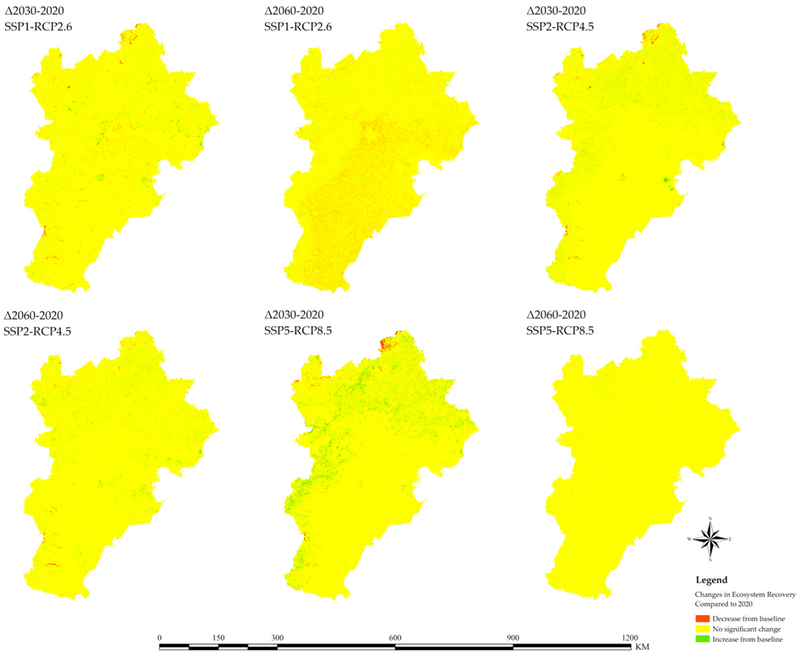
3.2.3. Spatio-Temporal Dynamics of Ecosystem Recovery Under Three SSP Scenarios

When examined from a temporal perspective, the average ecosystem recovery value in 2020 was 0.5891, and in the SSP1-2.6 and SSP5-8.5 scenarios, the mean ecosystem recovery values show a trend of 2030 > 2020 > 2060 (SSP1-2.6: 2030-0.5945, 2060-0.5872; SSP5-8.5: 2030-0.5922, 2060-0.5-8.57), indicating improved recovery from 2020 to 2030 and then weakened recovery from 2030 to 2060. The recovery ability is strongest in 2030. In SSP2-4.5, the average recovery values show a trend of 2060 > 2030 > 2020 (2030-0.5938, 2060-0.6017), indicating continuously increasing recovery ability from 2020 to 2060.

Comparing the ecosystem recovery values of different SSP scenarios at the same time point reveals the following: In 2030, the ranking of mean ecosystem recovery values for the BTH region is SSP1-2.6 (0.5945) > SSP2-4.5 (0.5938) > SSP5-8.5 (0.5922), indicating the strongest recovery under SSP1-2.6 and the weakest under SSP5-8.5. Conversely, in 2060, the ranking of average ecosystem recovery values for the BTH region is SSP2-4.5 (0.6017) > SSP1-2.6 (0.5872) > SSP5-8.5 (0.5857), indicating the strongest recovery under SSP2-4.5 and the weakest under SSP5-8.5.

The standard deviation analysis indicates an increasing spatial imbalance in ecosystem recovery from 2030 to 2060. The spatial distribution of ecosystem restoration in the BTH region exhibits significant variation, with clear natural transitions, and similar patterns are found in each group. The spatial pattern reveals distinct north–south differences in ecosystem recovery, with higher restoration levels observed in the northern mountainous regions compared to the plains in the south. Spatially, ecosystem recovery exhibits north–south differences, with higher recovery in northern mountainous regions and lower recovery in southern plains (Figure 10).

The differences in ecosystem recovery between 2020 and the projected years of 2030 and 2060 under the three SSP scenarios are illustrated in Figure 11.

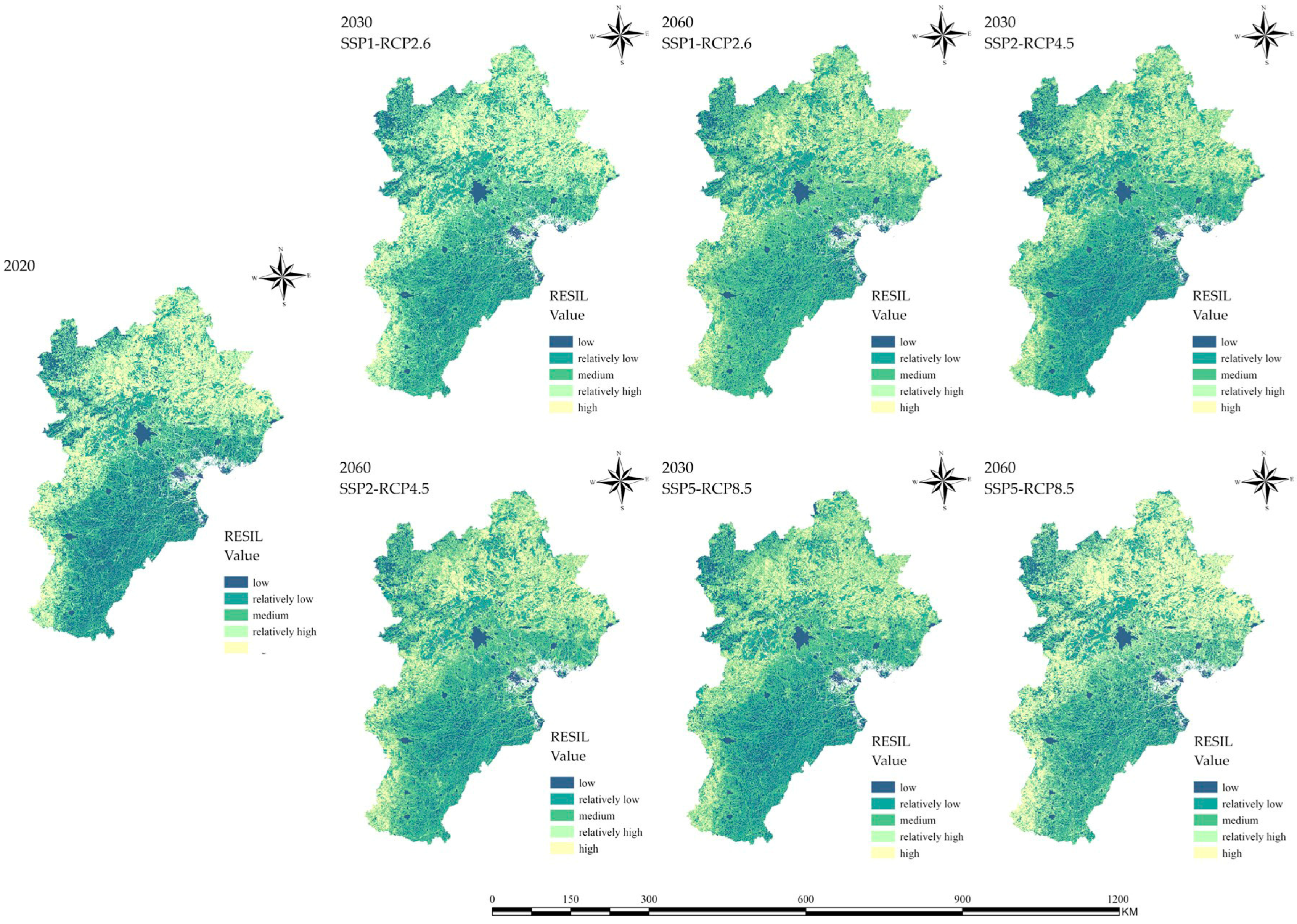
3.2.4. Spatio-Temporal Patterns of Ecosystem Resilience Under Three SSP Scenarios

The ecosystem resilience of the BTH region was calculated based on ecosystem resistance, adaptability, and recovery using Formula (10).

When examined from a temporal perspective, the average ecosystem resilience value in 2020 was 0.3259, and under SSP1-2.6, the average resilience values exhibit a trend of 2060 (0.3363) > 2030 (0.3361) > 2020, indicating continuously increasing resilience from 2020 to 2060. In the SSP2-4.5 and SSP5-8.5 scenarios, the average resilience values show a trend of 2060 > 2020 > 2030 (SSP2-4.5: 2030-0.3213, 2060-0.3361; SSP5-8.5: 2030-0.3259, 2060-0.3391), indicating weakened resilience from 2020 to 2030 and then improved resilience from 2030 to 2060. Resilience is the strongest in 2060.

Comparing the ecosystem resilience values in different SSP scenarios at the same time point reveals the following: In 2030, the ranking of the mean resilience values for the BTH region is SSP1-2.6 (0.3361) > SSP2-4.5 (0.3213) > SSP5-8.5 (0.3205), indicating the strongest resilience under SSP1-2.6 and the weakest under SSP5-8.5. In contrast, in 2060, the ranking of the mean resilience values for the BTH region is SSP5-8.5 (0.3391) > SSP1-2.6 (0.3363) > SSP2-4.5 (0.3361), indicating the strongest resilience under SSP5-8.5 and the weakest under SSP2-4.5.

The standard deviation analysis indicates a narrowing spatial imbalance in ecosystem resilience from 2030 to 2060, suggesting an increased spatial balance.

Over this period, the spatial distribution of resilience in the BTH region remains largely consistent, with lower resilience in the central, southeastern, and northwestern regions and higher resilience in the northeastern and southwestern parts, particularly in mountainous regions with forests and grasslands. Notably, the lowest resilience is observed in Beijing’s core construction zones and the Bohai Bay area (Figure 12).

The differences in ecosystem resilience between 2020 and the projected years of 2030 and 2060 under the three SSP scenarios are illustrated in Figure 13.

3.3. Distribution and Characteristics of Ecosystem Resilience Management Zones

Over this period, the spatial distribution of resilience in the BTH region remains largely consistent, with lower resilience in the central, southeastern, and northwestern regions and higher resilience in the northeastern and southwestern parts, particularly in mountainous regions with forests and grasslands. Notably, the lowest resilience is observed in Beijing’s core construction zones and the Bohai Bay area (Figure 14).

(1)

The core ecological protection zone has the highest ecosystem resilience, a stable ecosystem, rich biodiversity, and important ecosystem service functions. It is predominantly located in the most forested mountainous areas of northeastern and southwestern BTH, characterized by high ecosystem resilience. Examples include the Yanshan Mountain Water Conservation and Soil Retention Area and the Taihang Mountain Water Conservation and Soil Retention Area.

(2)

The ecological optimization zone has relatively high ecosystem resilience but still has room for improvement. Some regions may be slightly affected by human activities, such as agriculture and low-density development. It is mainly distributed around the core ecological protection zone, located in a mixed distribution zone of mountainous forests, grasslands, and river valleys.

(3)

The ecological restoration zone has relatively low ecosystem resilience, and the ecosystem has been degraded to a certain degree. Areas of this type are scattered across the northeastern, southwestern, and northwestern parts of the BTH region, while they are more concentrated in the southeastern region, interspersed with small ecological vulnerability control areas. A key example of this area type is the North China Plain Ecological Restoration Zone, primarily composed of cultivated land and other land use types. As an artificial ecosystem, the agricultural landscape is highly susceptible to human activities, with limited self-recovery capacity.

(4)

The ecological vulnerability control zone represents areas with low ecosystem resilience that require focused conservation efforts. Covering a relatively small area, regions of this type are primarily distributed across the Bashang Plateau, the Bohai Bay area, and the central urbanized region of Beijing. The Bashang Plateau, a key ecological barrier in North China, faces major challenges, such as soil erosion, wind-blown sand, and drought [72,73]. The Bohai coastal region experiences ecosystem fragility due to coastal erosion and excessive development [74]. Meanwhile, the urban center in Beijing struggles with environmental degradation due to excessive land development. Strengthening ecological protection in the ecological vulnerability control zone is essential to optimizing ecological security and promoting sustainable regional development in the BTH region.

4. Discussion

4.1. The Spatio-Temporal Dynamics of Ecosystem Resilience to the Coupled Impacts of Climate and Land Use Changes

Our findings reveal significant spatio-temporal variations in ecosystem resilience across the BTH region under different SSP scenarios. We observed that, in each SSP scenario, ecosystem resilience values generally increased from 2030 to 2060. This trend likely reflects the projected positive impacts of land and environmental governance policies, such as afforestation and integrated ecosystem management, leading to optimized land use patterns and enhanced ecosystem services [75]. Contrasting trends emerged when comparing scenarios. Ecosystem resilience was generally the highest under SSP1-2.6, emphasizing sustainable development, and the lowest under SSP5-8.5, which prioritizes rapid economic growth with high emissions. This aligns with existing research [20,44,76] and highlights the vital role of socioeconomic pathways in shaping ecosystem resilience.

The spatial pattern of ecosystem resilience in the BTH region is shaped by the interplay of topography, land cover types, and human activity intensity. Areas of high resilience are predominantly located in mountainous and semi-mountainous zones, such as the Yanshan and Taihang ranges, which are characterized by extensive forest and grassland coverage. These regions exhibit favorable ecological conditions, including a high vegetation density, a complex landscape structure, and reduced anthropogenic disturbances. As a result, they demonstrate superior performance in resistance, adaptability, and recovery dimensions of resilience.

Conversely, areas with low resilience are concentrated in the southeastern plains, the Bashang Plateau, and coastal zones along Bohai Bay. These regions are dominated by cultivated land, construction land, and water bodies and are subject to intensive human development, high population density, and significant ecological fragmentation. Such conditions undermine the ecological capacity to resist disturbances, recover from degradation, and maintain structural and functional integrity, leading to consistently lower resilience scores across scenarios. This spatial differentiation highlights the fundamental role of natural landscape features and land use patterns in determining ecosystem resilience. It also underscores the importance of tailoring regional management strategies to local ecological and socioeconomic contexts.

4.1.1. The Influence of Land Use Change on Future Ecosystem Resilience

Land use change is one of the most significant anthropogenic drivers shaping the dynamics of ecosystem resilience, as it directly alters the land cover composition, landscape configuration, and ecological functioning. As shown in Table 5, the BTH region is projected to experience substantial land use transitions in all SSP-RCP scenarios from 2020 to 2060. These changes are characterized by a general decline in cultivated land, the continuous expansion of construction land, and varying trends in forest and water bodies.

In 2030, the SSP1-2.6 scenario reflects moderate forest expansion and reduced construction land growth, supporting ecological restoration and water-related services. These transitions correspond to the highest resistance and overall resilience values among the three scenarios, demonstrating the positive effects of land protection policies. In 2060, SSP2-4.5 achieves the highest resistance and recovery values, benefiting from sustained forest growth and balanced urban expansion, which enhances water conservation, soil retention, and landscape continuity [77].

Conversely, SSP5-8.5 in 2060 shows the most significant loss of forestland (−456.31 km²) and aggressive urban expansion, contributing to ecosystem degradation in many areas. However, it also exhibits the highest adaptability score due to increased landscape fragmentation, which leads to more complex spatial configurations and higher edge densities. These features are captured by elevated values of PARA_AM and LSI, indicating structurally diverse, albeit stressed, landscapes. These results highlight that land use composition and landscape structure jointly influence ecosystem resilience outcomes and that managing urban growth, maintaining ecological corridors, and protecting natural land patches are key strategies to improve long-term resilience. Humid subregions benefit from increased rainfall, partially buffering the negative impact of forest loss.

The rapid growth of construction land, especially under SSP1-2.6 and SSP5-8.5, induces habitat fragmentation and spatial heterogeneity. This shift boosts adaptability scores, particularly in 2060 under SSP5-8.5 (0.3304), due to increases in landscape complexity indices such as PARA_AM and LSI. These indices capture irregular shapes and higher edge densities, which suggest a greater capacity for spatial reorganization but also signal ecological stress.

In terms of recovery, reductions in cultivated land and increases in forestland contribute to stronger regenerative capacity, particularly under SSP2-4.5 in 2060. This scenario balances urban growth with ecological restoration, leading to the highest recovery value and overall resilience.

Collectively, these results highlight that land use change influences resilience not only by directly modifying ecosystem components (e.g., forest loss or urban expansion) but also by altering spatial configuration and connectivity. The interaction between the land use composition and the landscape pattern determines the functional performance of ecosystems under future scenarios. Therefore, careful planning and land reallocation policies, such as protecting forest margins, restoring ecological corridors, and managing urban sprawl, are essential to sustaining long-term ecosystem resilience.

4.1.2. The Role of Climate Change in Shaping Future Ecosystem Resilience

Climate change acts as a systemic driver of ecosystem functioning, influencing resilience both directly through impacts on temperature, precipitation, and hydrological balance and indirectly via its modulation of land use and landscape transitions. In this study, resilience components such as water conservation (WC), soil retention (SC), and habitat quality (HQ) are all sensitive to the climate inputs modeled under the SSP-RCP pathways [78].

In 2030, SSP1-2.6 demonstrates the highest resilience, supported by moderate climate conditions (678.85 mm precipitation, 11.08 °C temperature), which promote ecological stability and service provision (

Table A1. Projected climate variables in the BTH region under different SSP-RCP scenarios (2030 and 2060).

Climate Variables	2030 (2020–2040)			2060 (2040–2060)
	SSP1-2.6	SSP2-4.5	SSP5-8.5	SSP1-2.6	SSP2-4.5	SSP5-8.5
Projected Mean Precipitation (mm)	678.8516	681.3850	663.5665	710.2390	736.4845	748.0945
Standard Deviation of Precipitation	98.8285	109.0324	93.8055	114.5788	104.7520	113.8589
Projected Mean Temperature (°C)	11.0836	11.2400	11.5809	11.5665	12.0984	12.5428
Standard Deviation of Temperature	3.5100	3.4644	3.4873	3.5761	3.5277	3.5060

). The relatively mild temperature favors plant productivity and microbial processes, enhancing nutrient cycling and biomass accumulation, which are beneficial for ecosystem resilience. In contrast, SSP5-8.5, under drier and more variable conditions, results in lower resilience despite comparable land use inputs.

However, in 2060, the pattern shifts due to a significant increase in projected precipitation under SSP5-8.5 (748.09 mm, the highest among the scenarios), alongside the greatest spatial variance. In addition, the projected mean temperature under SSP5-8.5 reaches 12.54 °C—the highest among all scenarios (Table A1). This elevated temperature may accelerate plant growth and microbial activity, enhancing ecological processes such as carbon cycling and biomass accumulation in temperature-limited areas. This localized surge in rainfall likely enhances hydrological functions in humidified subregions, boosting WC and SC and partly offsetting the degradation associated with intensive development [79]. Nevertheless, in already heat-sensitive or water-stressed regions, increased temperature could intensify evapotranspiration, lower soil moisture retention, and stress native species, thereby acting as an ecological stressor. These dual effects indicate that temperature plays a context-dependent role in shaping future ecosystem resilience. These findings confirm that climate-induced resilience responses are nonlinear and spatially heterogeneous, with high rainfall variability potentially enabling short-term ecological gains in specific contexts (detailed in Section 4.1.3). Hence, integrating both temperature and precipitation trends is essential for capturing the full range of climate impacts on ecosystem resilience, especially under high-emission trajectories.

The climate impacts simulated in the model are based on average trends and selected direct inputs. However, incorporating a broader range of climate change effects, particularly extreme events and nonlinear ecological responses, is essential for improving the reliability of future projections, especially in high-emission scenarios.

4.1.3. Interpreting the Unexpected Resilience Peak Under SSP5-8.5 in 2060

The highest overall resilience observed under the SSP5-8.5 scenario in 2060 appears counterintuitive, given this scenario’s association with high greenhouse gas emissions, environmental degradation, and rapid urban expansion. This anomaly may be attributed to a combination of short-term ecological mechanisms and structural assumptions within the modeling framework and should therefore be interpreted with caution.

Firstly, SSP5-8.5 projects the highest annual precipitation and the greatest climatic variability across the BTH region, as shown in Table A1. Increased rainfall may enhance hydrological regulation and soil retention in certain fragmented yet humid subregions that retain ecological restoration potential [80]. This may disproportionately elevate the resistance component in this scenario. However, these benefits are likely temporary and spatially heterogeneous, and the model does not consider long-term stress accumulation or the effects of extreme weather events. Furthermore, the projected mean temperature in 2060 under SSP5-8.5 is 12.54 °C, the highest among all scenarios. This warming may stimulate biological activity and reinforce ecosystem processes in certain temperature-limited areas, further contributing to the rise in resistance. However, this effect is likely uneven and could be counteracted by elevated evapotranspiration or heat-induced habitat stress in already vulnerable regions.

Secondly, the land use dynamics under SSP5-8.5 result in highly fragmented landscapes, which increase spatial heterogeneity and complexity. This structural complexity is reflected in the highest adaptability score among the scenarios, supported by elevated values of PARA_AM and LSI. These metrics indicate the potential for ecological reorganization. Nonetheless, increased fragmentation may also lead to negative ecological outcomes, such as reduced landscape connectivity, intensified edge effects, and the degradation of core habitats. Such effects are not fully captured by the current adaptability indicators, which mainly reflect the spatial configuration rather than the functional capacity.

Although the recovery score under SSP5-8.5 is not the highest, the combined increase in resistance and adaptability contributes to the scenario’s overall resilience ranking. However, this outcome may be influenced by limitations within the modeling system, such as the assumption of static carbon densities, the simplified representation of recovery processes, and the absence of extreme climate variables. Additionally, the model’s treatment of temperature relies on annual mean values and does not account for potential thresholds, nonlinear ecological stress, or temperature-driven tipping points. In addition, the weighting scheme of resilience components may amplify the spatial structure while underestimating latent ecological risks.

Overall, the peak resilience value observed in 2060 under SSP5-8.5 should be treated as a warning signal rather than an indication of sustainable improvement. This result highlights the complex and potentially nonlinear nature of ecosystem responses and reinforces the importance of incorporating connectivity, disturbance regimes, and long-term degradation thresholds in future modeling efforts to better assess resilience under high-emission scenarios (detailed in Section 4.3) [81].

In conclusion, climate conditions and land use change emerged as key drivers of ecosystem resilience variations across scenarios and time. Climate variables, especially precipitation and temperature, directly influence the provision of ecosystem services (resistance) by altering ecological processes [11]. Land use changes, driven by human activities and policies, directly impact ecosystem structure and functions, indirectly affecting resistance, adaptability (landscape patterns), and recovery [82]. Human activities, mediated through land use and climate change, are ultimately the primary modifiers of ecosystem resilience. As resilience is intrinsically linked to human well-being, adaptive development strategies and policies are crucial [83]. Our findings highlight the need for spatially differentiated management approaches, tailored to local resilience levels and future scenarios, to achieve ecologically sustainable development in the BTH region.

4.2. Management Strategies and Policy Implications of Ecological Management Zones

Human activities, mediated through land use and climate change, are ultimately the primary modifiers of ecosystem resilience. As resilience is intrinsically linked to human well-being, adaptive development strategies and policies are crucial [83]. Our findings highlight the need for spatially differentiated management approaches, tailored to local resilience levels and future scenarios, to achieve ecologically sustainable development in the BTH region. Based on our research results, reasonable management strategies and policies that consider the coupled impacts of land use and climate change should be formulated for ecosystem management in the BTH region. Due to variations in the natural background and the degree of socioeconomic influence, ecosystem development varies among different regions. Therefore, region-specific management strategies should be adopted for different zones. This differentiation will help implement tailored and refined conservation strategies, thereby enhancing ecosystem resilience, ensuring healthy and stable regional development, and promoting the sustainable use of ecological resources. Based on the characteristics and distribution of different ecological management zones (Figure 9), the following management recommendations are proposed for future ecosystem protection zones in the BTH region (Figure 15).

4.2.1. Core Ecological Protection Zone

The core ecological protection zone, which maintains a well-preserved original ecosystem structure and strong ecological functions, is characterized by the highest ecosystem resilience value. To sustain the existing natural environment, it is essential to limit human activities and allow the ecosystem to undergo natural renewal and succession. Ecological security reserves should be established, with the Yanshan Mountain Water Conservation and Soil Retention Area and the Taihang Mountain Water Conservation and Soil Retention Area as the core. Human development should be restricted, and ecological red-line management should be implemented to prevent land use changes from damaging ecosystems. A long-term ecological monitoring system should be established to assess changes in ecological functions and ensure ecosystem stability. Additionally, an ecological compensation mechanism should be introduced to provide economic incentives for local communities, encouraging sustainable development practices such as eco-tourism and sustainable agriculture.

4.2.2. Ecological Optimization Zone

The ecosystem in the ecological optimization zone exhibits strong functionality and relatively high resilience but may face certain ecological pressures, such as soil erosion and habitat fragmentation. With proper management and ecological restoration, its functions have the potential to be further enhanced. The management strategy for this region should focus on promoting Low-Impact Development (LID) and sustainable agriculture, such as reducing the use of pesticides and chemical fertilizers while promoting ecological farming practices. Measures such as establishing ecological corridors and restoring wetlands should be implemented to enhance biodiversity and improve the connectivity of ecological networks. Additionally, fostering environmentally friendly industries, including eco-tourism and the green economy, can boost regional economic benefits while minimizing ecological degradation.

4.2.3. Ecological Restoration Zone

The dominant land use in this area is cultivated land, and the ecosystem exhibits relatively low resilience. Some areas are already experiencing land degradation and resource overuse, resulting in impaired ecological functions, such as diminished soil and water conservation ability, decreasing biodiversity, and diminished carbon storage. To address these issues, ecological restoration and effective management measures are necessary to enhance the ecosystem’s recovery capacity. The protection of the local ecosystem should involve measures such as afforestation, grassland restoration, and the conversion of farmland back to forests and grasslands to improve land quality and ecological functions. Pollution control should be integrated with ecological restoration by implementing watershed management strategies to reduce water pollution while restoring key ecosystems such as wetlands and rivers. Additionally, promoting ecological agriculture and transitioning to sustainable industries can enhance local farmers’ awareness of sustainable development while increasing their economic benefits.

4.2.4. Ecological Vulnerability Control Zone

This region has the lowest ecological resilience, with a highly fragile ecosystem facing severe environmental pressures, such as overgrazing and desertification (Bashang Plateau), coastal erosion (along the Bohai Bay area), and significant human-induced disturbances, such as urban expansion in central Beijing. Due to the high difficulty of ecological restoration, targeted risk prevention and control measures are necessary to mitigate ecological degradation and reduce the impact of environmental disasters. The management strategy for this region should focus on establishing an ecological disaster prevention and mitigation system to enhance the ecosystem’s resilience to disasters. Strictly controlling overdevelopment, limiting groundwater extraction, and relocating non-capital functions from urban centers can help reduce the human impact on the environment. Additionally, policy support should be leveraged to guide population migration from highly fragile areas to regions with sustainable development potential while promoting a transition to a green economy.

This zoning strategy provides a valuable reference for setting ecological management goals and priorities for the near-medium and long term. In the near-medium term, efforts should focus on addressing the pronounced polarization of ecosystem resilience and the overall low resilience levels. This includes optimizing land use structure, restricting uncontrolled urban expansion, and enhancing preparedness for extreme climate events. In the long term, the key challenge lies in preventing the spread of high-risk ecological zones from the Bashang Plateau toward the BTH urban center. Therefore, strengthening the ecological barrier function of the Bashang Plateau, enhancing soil and water conservation efforts in the region, and optimizing Beijing’s industrial structure are of great significance [84]. Additionally, appropriate ecological protection policies should be implemented to mitigate ecosystem degradation in Beijing.

4.3. Limitations and Future Research

This study has certain limitations and uncertainties that require further attention in future research. Firstly, the land use predictions using the SD model considered only four key subsystems—population, climate, economy, and land use—to predict land use data in the BTH region for 2030 and 2060 based on their interdependencies. However, this does not suggest that other elements lack an impact on land use. Additional subsystems, such as infrastructures and ecological and land use policies, should be comprehensively incorporated to improve precision in land use prediction. Secondly, for the resistance module of ecosystem resilience, ecological recovery capacity was evaluated by considering only four key ecosystem services: WC, SC, HQ, and CS. To refine and expand the assessment, it is recommended that more comprehensive service types be incorporated in the future. Lastly, we used key climate indicators, such as annual precipitation and mean temperature, to analyze the impact of climate change on ecosystem resilience. However, this study did not account for the mechanisms through which extreme climate events, such as droughts, floods, and heatwaves, may affect ecosystem functioning and resilience. This limitation is particularly important in light of the unexpected result observed in 2060, where the SSP5-8.5 scenario, despite projecting the most severe climate trajectory, exhibits the highest ecosystem resilience. This counterintuitive outcome suggests that the absence of extreme climate event variables may obscure critical stress-response dynamics and limit the explanatory power of the model.

Future research should explicitly incorporate extreme events as driving variables, alongside long-term climatic trends, in order to more accurately capture the compound pressures that ecosystems may face. Additionally, future work should consider refining the selection of resilience indicators, integrating socioeconomic and policy dimensions, and constructing a multidimensional, process-based resilience assessment framework. These improvements would enable a more comprehensive and realistic prediction of regional ecosystem resilience under complex and evolving environmental conditions.

In addition, some of the input variables used in this study, such as night-time light intensity (500 m), precipitation and precipitation erosivity (1 km), and future GDP and urbanization ratio (5 km), differ in spatial resolution from the 100 m base resolution employed in the simulation. To maintain spatial consistency, all datasets were resampled to 100 m using bilinear or nearest-neighbor interpolation, depending on the data type. While this approach enables integrated modeling, we acknowledge that the resampling process may introduce uncertainties, particularly in areas with sharp gradients or heterogeneous features. Future work could benefit from the use of higher-resolution socioeconomic and climatic projections or uncertainty quantification methods to better assess the influence of input data resolution on simulation outcomes.

5. Conclusions

This study established an assessment and projection framework for ecosystem resilience under future SSP-RCP scenarios based on multi-source remote sensing data, in order to explore the coupled impacts of climate change and land use transformation on ecosystem recovery in the BTH region. Additionally, an ecological management zoning strategy has been formulated for the near-medium and long-term periods. This study reveals significant temporal dynamics in ecosystem resilience in the BTH region, with projected resilience values in 2060 notably exceeding those in 2030. Moreover, within specific timeframes, the ecosystem resilience under different SSP scenarios exhibits a discernible trend, generally ranking as follows: SSP1-2.6 > SSP2-4.5 > SSP5-8.5. However, in 2060, an unusual pattern of SSP5-8.5 > SSP1-2.6 > SSP2-4.5 was observed, which is speculated to have resulted from the influence of extreme climate events under the high-emission scenario. The spatial distribution of ecosystem resilience exhibits a consistent pattern, with lower resilience observed in Beijing’s urban center, the southeastern plains, the Bohai Bay area, and the Bashang Plateau in the northwest. In contrast, higher resilience is found in the forested mountainous regions of the northeast and southwest. This study indicates that climate change and land use jointly influence changes in future ecosystem resilience. Variables related to the climate—particularly rainfall and temperature—play a pivotal role in shaping ecosystem services (resistance) by influencing ecological mechanisms. At the same time, shifts in land use practices have a profound impact on both the composition and operational dynamics of ecosystems, which in turn have indirect effects on resistance, landscape patterns (adaptability), and recovery. According to the presented ecological management zoning strategy, we recommend the rational planning of land use spatial patterns to avoid the degradation of ecosystem resilience. It is essential to conduct real-time monitoring of climate change, promptly detect extreme weather events, optimize land use patterns, and formulate reasonable land development and ecological management policies to enhance land quality and ecological functions. In summary, this study provides a spatially explicit analysis of the coupled impacts of climate and land use changes on ecosystem resilience in the BTH region under different SSP-RCP scenarios. We find a general trend of decreasing resilience, particularly around major urban centers, highlighting the need for strategic planning. However, the complex interplay of factors under the high-emission SSP5-8.5 scenario resulted in a projected increase in overall resilience by 2060, a finding that underscores the intricate and sometimes counter-intuitive ways climate and land use changes interact and points to the need for further investigation using more dynamic and process-based models. The proposed ecological management zones offer a differentiated approach to future ecological conservation and restoration, providing spatially explicit guidance for policy-making. Overall, this study highlights the value of integrating remote sensing and scenario-based simulation for ecosystem resilience assessment, offering practical insights for adaptive landscape governance under future uncertainties.

References

1. Baumgaertner, S.; Strunz, S. The Economic Insurance Value of Ecosystem Resilience. Ecol. Econ. 2014, 101, 21–32. [Google Scholar] [CrossRef]
2. Holling, C.S. Resilience and Stability of Ecological Systems; Cambridge University Press: Cambridge, UK, 2022. [Google Scholar]
3. Liu, X.; Li, Z.; Wang, T.; Cheng, S.; Zheng, X.; Jia, L.; Liu, B.; Li, J.; Miao, Z. The Change of Ecosystem Resilience and Its Response to Economic Factors in Yulin, China. Environ. Res. Commun. 2023, 5, 45006. [Google Scholar] [CrossRef]
4. Xu, X.; Wang, M.; Wang, M.; Yang, Y.; Wang, Y. The Coupling Coordination Degree of Economic, Social and Ecological Resilience of Urban Agglomerations in China. Int. J. Environ. Res. Public Health 2022, 20, 413. [Google Scholar] [CrossRef] [PubMed]
5. Sterk, M.; Gort, G.; Klimkowska, A.; Van Ruijven, J.; Van Teeffelen, A.J.A.; Wamelink, G.W.W. Assess Ecosystem Resilience: Linking Response and Effect Traits to Environmental Variability. Ecol. Indic. 2013, 30, 21–27. [Google Scholar] [CrossRef]
6. Zheng, S.; Yang, S.; Ma, M.; Dong, J.; Han, B.; Wang, J. Linking Cultural Ecosystem Service and Urban Ecological-Space Planning for a Sustainable City: Case Study of the Core Areas of Beijing under the Context of Urban Relieving and Renewal. Sustain. Cities Soc. 2023, 89, 104292. [Google Scholar] [CrossRef]
7. Li, B.; Li, X.; Liu, C. Dynamic Evolution of the Ecological Resilience and Response under the Context of Carbon Neutrality. Ecosyst. Health Sustain. 2023, 9, 130. [Google Scholar] [CrossRef]
8. Li, J.; Nie, W.; Zhang, M.; Wang, L.; Dong, H.; Xu, B. Assessment and Optimization of Urban Ecological Network Resilience Based on Disturbance Scenario Simulations: A Case Study of Nanjing City. J. Clean. Prod. 2024, 438, 140812. [Google Scholar] [CrossRef]
9. Jie, Y.; Shiying, W.; Jie, Z.; Jing, Z.; Wenliu, Z. Optimisation of Ecological Security Patterns in Ecologically Transition Areas under the Perspective of Ecological Resilience—A Case of Taohe River. Ecol. Indic. 2024, 166, 112315. [Google Scholar] [CrossRef]
10. Li, D.; Meng, W.; Liu, B.; Xu, W.; Hu, B.; Huang, Z.; Lu, Y. Temporal-Spatial Change of China’s Coastal Ecosystem Resilience and Driving Factors Analysis. Ocean Coast. Manag. 2024, 255, 107209. [Google Scholar] [CrossRef]
11. Yan, H.; Zhan, J.; Liu, B.; Huang, W.; Li, Z. Spatially Explicit Assessment of Ecosystem Resilience: An Approach to Adapt to Climate Changes. Adv. Meteorol. 2014, 2014, 1–9. [Google Scholar] [CrossRef]
12. Zhao, R.; Fang, C.; Liu, H.; Liu, X. Evaluating Urban Ecosystem Resilience Using the DPSIR Framework and the ENA Model: A Case Study of 35 Cities in China. Sustain. Cities Soc. 2021, 72, 102997. [Google Scholar] [CrossRef]
13. Liao, L.; Ma, E.; Long, H.; Peng, X. Land Use Transition and Its Ecosystem Resilience Response in China during 1990–2020. Land 2022, 12, 141. [Google Scholar] [CrossRef]
14. Feng, Y.; Lei, Z.; Tong, X.; Gao, C.; Chen, S.; Wang, J.; Wang, S. Spatially-Explicit Modeling and Intensity Analysis of China’s Land Use Change 2000–2050. J. Environ. Manag. 2020, 263, 110407. [Google Scholar] [CrossRef] [PubMed]
15. Meng, Z.; He, M.; Li, X.; Li, H.; Tan, Y.; Li, Z.; Wei, Y. Spatio-temporal Analysis and Driving Forces of Urban Ecosystem Resilience Based on Land Use: A Case Study in the Great Bay Area. Ecol. Indic. 2024, 159, 111769. [Google Scholar] [CrossRef]
16. Baho, D.L.; Allen, C.R.; Garmestani, A.; Fried-Petersen, H.; Renes, S.E.; Gunderson, L.; Angeler, D.G. A Quantitative Framework for Assessing Ecological Resilience. Ecol. Soc. 2017, 22, art17. [Google Scholar] [CrossRef] [PubMed]
17. Ingrisch, J.; Bahn, M. Towards a Comparable Quantification of Resilience. Trends Ecol. Evol. 2018, 33, 251–259. [Google Scholar] [CrossRef] [PubMed]
18. Duo, L.; Li, Y.; Zhang, M.; Zhao, Y.; Wu, Z.; Zhao, D. Spatiotemporal Pattern Evolution of Urban Ecosystem Resilience Based on “Resistance-Adaptation-Vitality”: A Case Study of Nanchang City. Front. Earth Sci. 2022, 10, 902444. [Google Scholar] [CrossRef]
19. Liang, X.; Guan, Q.; Clarke, K.C.; Liu, S.; Wang, B.; Yao, Y. Understanding the Drivers of Sustainable Land Expansion Using a Patch-Generating Land Use Simulation (PLUS) Model: A Case Study in Wuhan, China. Comput. Environ. Urban Syst. 2021, 85, 101569. [Google Scholar] [CrossRef]
20. Wan, Z.; Zhao, C.; Zhu, J.; Ma, X.; Chen, J.; Wang, J. Assessment and Prediction of Coastal Ecological Resilience Based on the Pressure–State–Response (PSR) Model. Land 2024, 13, 2130. [Google Scholar] [CrossRef]
21. Xia, C.; Dong, Z.; Chen, B. Spatio-temporal analysis and simulation of urban ecological resilience: A case study of Hangzhou. Acta Ecol. Sin. 2021, 42, 116–126. [Google Scholar] [CrossRef]
22. Griffith, G.P.; Hop, H.; Vihtakari, M.; Wold, A.; Kalhagen, K.; Gabrielsen, G.W. Ecological Resilience of Arctic Marine Food Webs to Climate Change. Nat. Clim. Change 2019, 9, 868–872. [Google Scholar] [CrossRef]
23. Li, Y.; Xiao, J.; Cong, N.; Yu, X.; Lin, Y.; Liu, T.; Qi, G.; Ren, P. Modeling Ecological Resilience of Alpine Forest under Climate Change in Western Sichuan. Forests 2023, 14, 1769. [Google Scholar] [CrossRef]
24. Pörtner, H.-O.; Roberts, D.C.; Tignor, M.M.B.; Poloczanska, E.S.; Mintenbeck, K.; Alegría, A.; Craig, M.; Langsdorf, S.; Löschke, S.; Möller, V.; et al. (Eds.) Climate Change 2022: Impacts, Adaptation and Vulnerability. Contribution of Working Group II to the Sixth Assessment Report of the Intergovernmental Panel on Climate Change; Cambridge University Press: Cambridge, UK, 2022. [Google Scholar]
25. Qin, J.; Hao, X.; Hua, D.; Hao, H. Assessment of Ecosystem Resilience in Central Asia. J. Arid Environ. 2021, 195, 104625. [Google Scholar] [CrossRef]
26. Eyring, V.; Bony, S.; Meehl, G.A.; Senior, C.A.; Stevens, B.; Stouffer, R.J.; Taylor, K.E. Overview of the Coupled Model Intercomparison Project Phase 6 (CMIP6) Experimental Design and Organization. Geosci. Model Dev. 2016, 9, 1937–1958. [Google Scholar] [CrossRef]
27. Bayar, A.S.; Yılmaz, M.T.; Yücel, İ.; Dirmeyer, P. CMIP6 Earth System Models Project Greater Acceleration of Climate Zone Change Due to Stronger Warming Rates. Earth’s Future 2023, 11, e2022EF002972. [Google Scholar] [CrossRef]
28. Chen, G.; Li, X.; Liu, X. Global Land Projection Based on Plant Functional Types with a 1-Km Resolution under Socio-Climatic Scenarios. Sci. Data 2022, 9, 125. [Google Scholar] [CrossRef] [PubMed]
29. Wang, Z.; Li, X.; Mao, Y.; Li, L.; Wang, X.; Lin, Q. Dynamic Simulation of Land Use Change and Assessment of Carbon Storage Based on Climate Change Scenarios at the City Level: A Case Study of Bortala, China. Ecol. Indic. 2022, 134, 108499. [Google Scholar] [CrossRef]
30. Yang, S.; Zhao, B.; Yang, D.; Wang, T.; Yang, Y.; Ma, T.; Santisirisomboon, J. Future Changes in Water Resources, Floods and Droughts under the Joint Impact of Climate and Land-Use Changes in the Chao Phraya Basin, Thailand. J. Hydrol. 2023, 620, 129454. [Google Scholar] [CrossRef]
31. Li, G.; Wang, W.; Li, B.; Duan, Z.; Hu, L.; Liu, J. Spatiotemporal Simulation of Blue-Green Space Pattern Evolution and Carbon Storage under Different SSP-RCP Scenarios in Wuhan. Sci. Rep. 2025, 15, 4017. [Google Scholar] [CrossRef] [PubMed]
32. Gao, J.; Gong, J.; Li, Y.; Yang, J.; Liang, X. Ecological Network Assessment in Dynamic Landscapes: Multi-Scenario Simulation and Conservation Priority Analysis. Land Use Policy 2024, 139, 107059. [Google Scholar] [CrossRef]
33. Su, B.; Huang, J.; Mondal, S.K.; Zhai, J.; Wang, Y.; Wen, S.; Gao, M.; Lv, Y.; Jiang, S.; Jiang, T.; et al. Insight from CMIP6 SSP-RCP Scenarios for Future Drought Characteristics in China. Atmos. Res. 2021, 250, 105375. [Google Scholar] [CrossRef]
34. O’Neill, B.C.; Carter, T.R.; Ebi, K.; Harrison, P.A.; Kemp-Benedict, E.; Kok, K.; Kriegler, E.; Preston, B.L.; Riahi, K.; Sillmann, J.; et al. Achievements and Needs for the Climate Change Scenario Framework. Nat. Clim. Change 2020, 10, 1074–1084. [Google Scholar] [CrossRef] [PubMed]
35. Tian, L.; Tao, Y.; Fu, W.; Li, T.; Ren, F.; Li, M. Dynamic Simulation of Land Use/Cover Change and Assessment of Forest Ecosystem Carbon Storage under Climate Change Scenarios in Guangdong Province, China. Remote Sens. 2022, 14, 2330. [Google Scholar] [CrossRef]
36. Zhang, S.; Yang, P.; Xia, J.; Wang, W.; Cai, W.; Chen, N.; Hu, S.; Luo, X.; Li, J.; Zhan, C. Land Use/Land Cover Prediction and Analysis of the Middle Reaches of the Yangtze River under Different Scenarios. Sci. Total Environ. 2022, 833, 155238. [Google Scholar] [CrossRef] [PubMed]
37. Li, S.; Cao, Y.; Liu, J.; Wang, S. Simulating Land Use Change for Sustainable Land Management in China’s Coal Resource-Based Cities under Different Scenarios. Sci. Total Environ. 2024, 916, 170126. [Google Scholar] [CrossRef] [PubMed]
38. Xu, X.; Kong, W.; Wang, L.; Wang, T.; Luo, P.; Cui, J. A Novel and Dynamic Land Use/Cover Change Research Framework Based on an Improved PLUS Model and a Fuzzy Multiobjective Programming Model. Ecol. Inf. 2024, 80, 102460. [Google Scholar] [CrossRef]
39. Yu, Y.; Guo, B.; Wang, C.; Zang, W.; Huang, X.; Wu, Z.; Xu, M.; Zhou, K.; Li, J.; Yang, Y. Carbon Storage Simulation and Analysis in Beijing-Tianjin-Hebei Region Based on CA-plus Model under Dual-Carbon Background. Geomat. Nat. Hazards Risk 2023, 14, 2173661. [Google Scholar] [CrossRef]
40. Li, X.; Fu, J.; Jiang, D.; Lin, G.; Cao, C. Land Use Optimization in Ningbo City with a Coupled GA and PLUS Model. J. Clean. Prod. 2022, 375, 134004. [Google Scholar] [CrossRef]
41. Liu, X.; Liang, X.; Li, X.; Xu, X.; Ou, J.; Chen, Y.; Li, S.; Wang, S.; Pei, F. A Future Land Use Simulation Model (FLUS) for Simulating Multiple Land Use Scenarios by Coupling Human and Natural Effects. Landsc. Urban Plan. 2017, 168, 94–116. [Google Scholar] [CrossRef]
42. Nie, W.; Xu, B.; Yang, F.; Shi, Y.; Liu, B.; Wu, R.; Lin, W.; Pei, H.; Bao, Z. Simulating Future Land Use by Coupling Ecological Security Patterns and Multiple Scenarios. Sci. Total Environ. 2023, 859, 160262. [Google Scholar] [CrossRef] [PubMed]
43. Sasaki, T.; Furukawa, T.; Iwasaki, Y.; Seto, M.; Mori, A.S. Perspectives for Ecosystem Management Based on Ecosystem Resilience and Ecological Thresholds against Multiple and Stochastic Disturbances. Ecol. Indic. 2015, 57, 395–408. [Google Scholar] [CrossRef]
44. Yao, Y.; Liu, Y.; Fu, F.; Song, J.; Wang, Y.; Han, Y.; Wu, T.; Fu, B. Declined Terrestrial Ecosystem Resilience. Glob. Change Biol. 2024, 30, e17291. [Google Scholar] [CrossRef] [PubMed]
45. Cote, I.M.; Darling, E.S. Rethinking Ecosystem Resilience in the Face of Climate Change. PLoS Biol. 2010, 8, e1000438. [Google Scholar] [CrossRef] [PubMed]
46. Sharp, R.; Tallis, H.; Ricketts, T.; Guerry, A.; Wood, S.; Chaplin-Kramer, R.; Nelson, E.; Ennaanay, D.; Wolny, S.; Olwero, N. InVEST User’s Guide; The Natural Capital Project: Stanford, CA, USA, 2018; Available online: https://naturalcapitalproject.stanford.edu/software/invest (accessed on 7 December 2024).
47. Budyko, M.I.; Miller, D.H. Climate and Life; Academic Press: New York, NY, USA, 1974. [Google Scholar]
48. Li, M.; Liang, D.; Xia, J.; Song, J.; Cheng, D.; Wu, J.; Cao, Y.; Sun, H.; Li, Q. Evaluation of Water Conservation Function of Danjiang River Basin in Qinling Mountains, China Based on InVEST Model. J. Environ. Manag. 2021, 286, 112212. [Google Scholar] [CrossRef] [PubMed]
49. Wang, X.; Wu, J.; Liu, Y.; Hai, X.; Shanguan, Z.; Deng, L. Driving Factors of Ecosystem Services and Their Spatiotemporal Change Assessment Based on Land Use Types in the Loess Plateau. J. Environ. Manag. 2022, 311, 114835. [Google Scholar] [CrossRef] [PubMed]
50. Deng, G.; Jiang, H.; Zhu, S.; Wen, Y.; He, C.; Wang, X.; Sheng, L.; Guo, Y.; Cao, Y. Projecting the Response of Ecological Risk to Land Use/Land Cover Change in Ecologically Fragile Regions. Sci. Total Environ. 2024, 914, 169908. [Google Scholar] [CrossRef] [PubMed]
51. Zhu, C.; Zhang, X.; Zhou, M.; He, S.; Gan, M.; Yang, L.; Wang, K. Impacts of Urbanization and Landscape Pattern on Habitat Quality Using OLS and GWR Models in Hangzhou, China. Ecol. Indic. 2020, 117, 106654. [Google Scholar] [CrossRef]
52. Wei, Q.; Abudureheman, M.; Halike, A.; Yao, K.; Yao, L.; Tang, H.; Tuheti, B. Temporal and Spatial Variation Analysis of Habitat Quality on the PLUS-InVEST Model for Ebinur Lake Basin, China. Ecol. Indic. 2022, 145, 109632. [Google Scholar] [CrossRef]
53. Wu, L.; Sun, C.; Fan, F. Estimating the Characteristic Spatiotemporal Variation in Habitat Quality Using the InVEST Model—A Case Study from Guangdong–Hong Kong–Macao Greater Bay Area. Remote Sens. 2021, 13, 1008. [Google Scholar] [CrossRef]
54. Wu, X.; Shen, C.; Shi, L.; Wan, Y.; Ding, J.; Wen, Q. Spatio-Temporal Evolution Characteristics and Simulation Prediction of Carbon Storage: A Case Study in Sanjiangyuan Area, China. Ecol. Inf. 2024, 80, 102485. [Google Scholar] [CrossRef]
55. Zhao, M.; He, Z.; Du, J.; Chen, L.; Lin, P.; Fang, S. Assessing the Effects of Ecological Engineering on Carbon Storage by Linking the CA-Markov and InVEST Models. Ecol. Indic. 2019, 98, 29–38. [Google Scholar] [CrossRef]
56. Jia, Y.; Tang, L.; Xu, M.; Yang, X. Landscape Pattern Indices for Evaluating Urban Spatial Morphology—A Case Study of Chinese Cities. Ecol. Indic. 2019, 99, 27–37. [Google Scholar] [CrossRef]
57. Peng, J.; Liu, Y.; Wu, J.; Lv, H.; Hu, X. Linking Ecosystem Services and Landscape Patterns to Assess Urban Ecosystem Health: A Case Study in Shenzhen City, China. Landsc. Urban Plan. 2015, 143, 56–68. [Google Scholar] [CrossRef]
58. Tonetti, V.; Pena, J.C.; Scarpelli, M.; Sugai, L.; Barros, F.; Ribeiro Anunciação, P.; Marques Santos, P.; Tavares, A.; Ribeiro, M. Landscape Heterogeneity: Concepts, Quantification, Challenges and Future Perspectives. Environ. Conserv. 2023, 50, 83–92. [Google Scholar] [CrossRef]
59. Pascual-Hortal, L.; Saura, S. Comparison and Development of New Graph-Based Landscape Connectivity Indices: Towards the Priorization of Habitat Patches and Corridors for Conservation. Landsc. Ecol. 2006, 21, 959–967. [Google Scholar] [CrossRef]
60. Huang, Q.; Huang, J.; Zhan, Y.; Cui, W.; Yuan, Y. Using Landscape Indicators and Analytic Hierarchy Process (AHP) to Determine the Optimum Spatial Scale of Urban Land Use Patterns in Wuhan, China. Earth Sci. Inform. 2018, 11, 567–578. [Google Scholar] [CrossRef]
61. Jaeger, J.A.G. Landscape Division, Splitting Index, and Effective Mesh Size: New Measures of Landscape Fragmentation. Landsc. Ecol. 2000, 15, 115–130. [Google Scholar] [CrossRef]
62. Riitters, K.H.; O’Neill, R.V.; Wickham, J.D.; Jones, K.B. A Note on Contagion Indices for Landscape Analysis. Landsc. Ecol. 1996, 11, 197–202. [Google Scholar] [CrossRef]
63. Ye, Y.; Qiu, H. Using Urban Landscape Pattern to Understand and Evaluate Infectious Disease Risk. Urban For. Urban Green. 2021, 62, 127126. [Google Scholar] [CrossRef] [PubMed]
64. Xiao, R.; Liu, Y.; Fei, X.; Yu, W.; Zhang, Z.; Meng, Q. Ecosystem Health Assessment: A Comprehensive and Detailed Analysis of the Case Study in Coastal Metropolitan Region, Eastern China. Ecol. Indic. 2019, 98, 363–376. [Google Scholar] [CrossRef]
65. Li, C.; Han, H.; Cui, N.; Lan, P.; Zhang, K.; Zhou, X.; Guo, L. Spatiotemporal Dynamics and Spatial Correlation Patterns of Urban Ecological Resilience across the Yellow River Basin in China. Sci. Rep. 2024, 14, 31286. [Google Scholar] [CrossRef] [PubMed]
66. Ji, X.; Nie, Z.; Wang, K.; Xu, M.; Fang, Y. Spatiotemporal Evolution and Influencing Factors of Urban Resilience in the Yellow River Basin, China. Reg. Sustain. 2024, 5, 100159. [Google Scholar] [CrossRef]
67. Mallick, S.K. Prediction-Adaptation-Resilience (PAR) Approach- A New Pathway towards Future Resilience and Sustainable Development of Urban Landscape. Geogr. Sustain. 2021, 2, 127–133. [Google Scholar] [CrossRef]
68. Cohen, J. A Coefficient of Agreement for Nominal Scales. Educ. Psychol. Meas. 1960, 20, 37–46. [Google Scholar] [CrossRef]
69. Foody, G.M. Status of Land Cover Classification Accuracy Assessment. Remote Sens. Environ. 2002, 80, 185–201. [Google Scholar] [CrossRef]
70. Pontius, R.G.; Millones, M. Death to Kappa: Birth of Quantity Disagreement and Allocation Disagreement for Accuracy Assessment. Int. J. Remote Sens. 2011, 32, 4407–4429. [Google Scholar] [CrossRef]
71. Singh, A. Review Article Digital Change Detection Techniques Using Remotely-Sensed Data. Int. J. Remote Sens. 1989, 10, 989–1003. [Google Scholar] [CrossRef]
72. Du, H.; Zhao, L.; Zhang, P.; Li, J.; Yu, S. Ecological Compensation in the Beijing-Tianjin-Hebei Region Based on Ecosystem Services Flow. J. Environ. Manag. 2023, 331, 117230. [Google Scholar] [CrossRef] [PubMed]
73. Zhu, L.; Ke, Y.; Hong, J.; Zhang, Y.; Pan, Y. Assessing Degradation of Lake Wetlands in Bashang Plateau, China Based on Long-Term Time Series Landsat Images Using Wetland Degradation Index. Ecol. Indic. 2022, 139, 108903. [Google Scholar] [CrossRef]
74. Li, S.; Wang, R.; Jiang, Y.; Li, Y.; Zhu, L.; Feng, J. Seasonal Variation of Food Web Structure and Stability of a Typical Artificial Reef Ecosystem in Bohai Sea, China. Front. Mar. Sci. 2022, 9, 830324. [Google Scholar] [CrossRef]
75. Chen, J.; Dong, Z.; Shi, R.; Sun, G.; Guo, Y.; Peng, Z.; Deng, M.; Chen, K. Urban Multi-Scenario Land Use Optimization Simulation Considering Local Climate Zones. Remote Sens. 2024, 16, 4342. [Google Scholar] [CrossRef]
76. Song, S.; Wang, S.; Gong, Y.; Yu, Y. The Past and Future Dynamics of Ecological Resilience and Its Spatial Response Analysis to Natural and Anthropogenic Factors in Southwest China with Typical Karst. Sci. Rep. 2024, 14, 19166. [Google Scholar] [CrossRef] [PubMed]
77. Wang, S.; Aihaiti, A.; Mamtimin, A.; Sayit, H.; Peng, J.; Liu, Y.; Wang, Y.; Gao, J.; Song, M.; Wen, C.; et al. Increases in Temperature and Precipitation in the Different Regions of the Tarim River Basin between 1961 and 2021 Show Spatial and Temporal Heterogeneity. Remote Sens. 2024, 16, 4612. [Google Scholar] [CrossRef]
78. Fang, W.; Qin, H.; Lin, Q.; Jia, B.; Yang, Y.; Shen, K. Deep Learning Integration of Multi-Model Forecast Precipitation Considering Long Lead Times. Remote Sens. 2024, 16, 4489. [Google Scholar] [CrossRef]
79. Li, Z.; Luo, S.; Tan, X.; Wang, J. Trend Analysis of High-Resolution Soil Moisture Data Based on GAN in the Three-River-Source Region during the 21st Century. Remote Sens. 2024, 16, 4367. [Google Scholar] [CrossRef]
80. Deng, Z.; Wang, Z.; Wu, X.; Lai, C.; Liu, W. Effect Difference of Climate Change and Urbanization on Extreme Precipitation over the Guangdong-Hong Kong-Macao Greater Bay Area. Atmos. Res. 2023, 282, 106514. [Google Scholar] [CrossRef]
81. Yao, Y.; Lu, L.; Guo, J.; Zhang, S.; Cheng, J.; Tariq, A.; Liang, D.; Hu, Y.; Li, Q. Spatially Explicit Assessments of Heat-Related Health Risks: A Literature Review. Remote Sens. 2024, 16, 4500. [Google Scholar] [CrossRef]
82. Hasan, S.S.; Zhen, L.; Miah, M.G.; Ahamed, T.; Samie, A. Impact of Land Use Change on Ecosystem Services: A Review. Environ. Dev. 2020, 34, 100527. [Google Scholar] [CrossRef]
83. Chaigneau, T.; Coulthard, S.; Daw, T.M.; Szaboova, L.; Camfield, L.; Chapin, F.S.; Gasper, D.; Gurney, G.G.; Hicks, C.C.; Ibrahim, M.; et al. Reconciling Well-Being and Resilience for Sustainable Development. Nat. Sustain. 2022, 5, 287–293. [Google Scholar] [CrossRef]
84. Wei, G.; He, B.-J.; Liu, Y.; Li, R. How Does Rapid Urban Construction Land Expansion Affect the Spatial Inequalities of Ecosystem Health in China? Evidence from the Country, Economic Regions and Urban Agglomerations. Environ. Impact Assess. Rev. 2024, 106, 107533. [Google Scholar] [CrossRef]
Figure 1. (a) The location of the study area. (b) Administrative divisions of the 13 cities included in the study area. (c) Elevation maps and three ecological functional conservation districts of the study area.
Remotesensing 17 02546 g001
Figure 2. Research framework.
Remotesensing 17 02546 g002
Figure 3. Causal feedback diagram of land use demand in the BTH region. (a) Stock and flow diagram of land use demand; (b) Causal structure of subsystem factors influencing land use demand.
Remotesensing 17 02546 g003
Figure 4. The spatial pattern of land use structure in 2020, 2030, and 2060 under the three SSP scenarios.
Remotesensing 17 02546 g004
Figure 5. Land use chord diagrams of the transition from 2020 to 2030 and 2060 in the three SSP scenarios.
Remotesensing 17 02546 g005
Figure 6. The spatial pattern of ecosystem resistance (RES) in 2020, 2030, and 2060 under the three SSP scenarios.
Remotesensing 17 02546 g006
Figure 7. Changes in ecosystem resistance (RES) in 2030 and 2060 compared to 2020 under the three SSP scenarios.
Remotesensing 17 02546 g007
Figure 8. The spatial pattern of ecosystem adaptability (ADA) in 2020, 2030, and 2060 under the three SSP scenarios.
Remotesensing 17 02546 g008
Figure 9. Changes in ecosystem adaptability (ADA) in 2030 and 2060 compared to 2020 under the three SSP scenarios.
Remotesensing 17 02546 g009
Figure 10. The spatial pattern of ecosystem recovery (REC) in 2020, 2030, and 2060 under the three SSP scenarios.
Remotesensing 17 02546 g010
Figure 11. Changes in ecosystem recovery (REC) in 2030 and 2060 compared to 2020 under the three SSP scenarios.
Remotesensing 17 02546 g011
Figure 12. The spatial distribution of ecosystem resilience (RESIL) in 2020, 2030, and 2060 under the three SSP scenarios.
Remotesensing 17 02546 g012
Figure 13. Changes in ecosystem resilience (RESIL) in 2030 and 2060 compared to 2020 under the three SSP scenarios.
Remotesensing 17 02546 g013
Figure 14. The distribution of ecological management zones in the near-medium (2030) term and long term (2060).
Remotesensing 17 02546 g014
Figure 15. Management strategies and policy implications.
Remotesensing 17 02546 g015