Optimizing the Sampling Strategy for Future Libera Radiance to Irradiance Conversions ^†

Abstract

The Earth Radiation Budget (ERB), a measure of the difference between incoming solar irradiance and outgoing reflected and emitted radiant energy, is a fundamental property of Earth’s climate system. The Libera satellite mission will measure the ERB’s outgoing components to continue the long-term climate data record established by NASA’s Clouds and the Earth’s Radiant Energy System (CERES) mission. In addition to ensuring data continuity, Libera will introduce a novel split-shortwave spectral channel to quantify the partitioning of the outgoing reflected solar component into visible and near-infrared sub-components. However, converting these split-shortwave radiances into the ERB-relevant irradiances requires the development of split-shortwave Angular Distribution Models (ADMs), which demand extensive angular sampling. Here, we show how Rotating Azimuthal Plane Scan (RAPS) parameters—specifically operational cadence and azimuthal scan rate—affect the observational coverage of a defined scene and angular space. Our results show that for a fixed number of azimuthal rotations, a relatively slow azimuthal scan rate of 0.5° per second, combined with more time spent in the RAPS observational mode, provides a more comprehensive sampling of the desired scene and angular space. We also show that operating the Libera instrument in RAPS mode at a cadence between every fifth day and every other day for the first year of space-based operations will provide sufficient scene and angular sampling for the observations to achieve radiance convergence for the scenes that comprise more than half of the expected Libera observations. Obtaining radiance convergence is necessary for accurate ADMs.

1. Introduction

One of the most fundamental properties of Earth’s climate system is the Earth Radiation Budget (ERB). The ERB is a measure of the difference between the incoming solar irradiance and outgoing irradiance from the Earth, which is composed of reflected solar (or shortwave) irradiance and the emitted terrestrial (or longwave) irradiance. Currently, the reference measurement of incoming solar irradiance is made by the Total and Spectral Solar Irradiance Sensor (TSIS-1) [1], while the reference measurement of the outgoing components is made by the Clouds and the Earth’s Radiance Energy System (CERES) [2,3]. These space-based measurements of the ERB aid the climate science community in quantifying when, where, and how Earth’s climate is changing [4]. An imbalance in the global ERB means there will be an overall response from the Earth’s climate, as manifested in recent changes such as increasing global mean surface temperatures [4], sea level rise [5], and more frequent extreme weather [6].

Measuring the outgoing irradiance is particularly challenging because the radiation field from Earth varies with solar-viewing geometry, wavelength, and scene composition [7]. This challenge has typically been addressed with wavelength- and scene-dependent Angular Distribution Models (ADMs) [8] that convert the measured directionally dependent radiances to hemispherically integrated irradiances, the energetically relevant quantity for the ERB. The CERES mission is approaching end-of-life, and its successor, Libera, will face the same radiance-to-irradiance conversion challenge. While Libera will provide continuity to the multidecade CERES climate data record, it will also introduce a new spectral band from 0.7 μm to 5 μm that splits the shortwave energy (incident at top-of-atmosphere) approximately in half. This split-shortwave channel aims to improve our insight into the shortwave absorption and scattering processes within the Earth–atmosphere system [9]. However, to achieve this goal, new split-shortwave ADMs are required to convert the measured split-shortwave radiance to irradiance.

To produce new split-shortwave ADMs, it is necessary to sample radiances across a wide range of solar-viewing geometries for different scene conditions. The Terra and Aqua satellites had two identical CERES instruments on each platform. One instrument typically operated in cross-track scanning mode, which is the nominal sampling pattern for generating the ERB climate data record, while the other operated in rotating azimuth plane scan (RAPS) mode, which allows for a broader range of observed angular space for ADM generation. This enabled the CERES instruments to collect multiple years of continuous observations in RAPS mode to develop ADMs while maintaining consistent cross-track observations throughout the missions. Libera is a single instrument and, therefore, cannot operate in multiple scan modes simultaneously. To address this challenge, Libera will fly a wide-field-of-view (WFOV) camera to assist with split-shortwave ADM development by providing angular sampling even when the radiometers are performing cross-track scans [10,11]. The Libera WFOV camera is a monochromatic camera that will operate at 555 nm with a 123° field of view and sub-kilometer pixel spacing at nadir, enabling continuous horizon-to-horizon imaging [11]. The idea is to spatially aggregate camera pixels up to the scale of the Libera footprint and apply a narrowband (555 nm) to broadband (VIS) conversion to provide proxy VIS radiometer footprints with dense angular sampling needed for ADM development [10]. However, the camera-based ADM approach is untested, so it is critical that some angular sampling is also acquired by the Libera split-shortwave radiometers for comparison and evaluation purposes. Thus, Libera has the challenge of balancing the amount and frequency of cross-track and RAPS observations. The goal of this study is to refine the partitioning between Libera cross-track and RAPS modes to minimize the amount of time spent in RAPS mode while achieving sufficient split-shortwave angular sampling.

A brief review of ADM theory is provided in Section 2. Section 3 describes the CERES RAPS data used in this study. Section 4 details the methodology and calculation sequence applied in the analysis. In Section 5, we use the CERES RAPS data to quantify the effect of RAPS cadence and scan rate on the observed angular space and the required sampling for radiance convergence. Conclusions are drawn in Section 6.

2. Theoretical Background for Converting Direct Measurements to Energy-Relevant Quantities

This section provides a brief overview of the theory behind ADMs and the scene types considered in this study, crucial for understanding the analysis and results discussed in the subsequent sections.

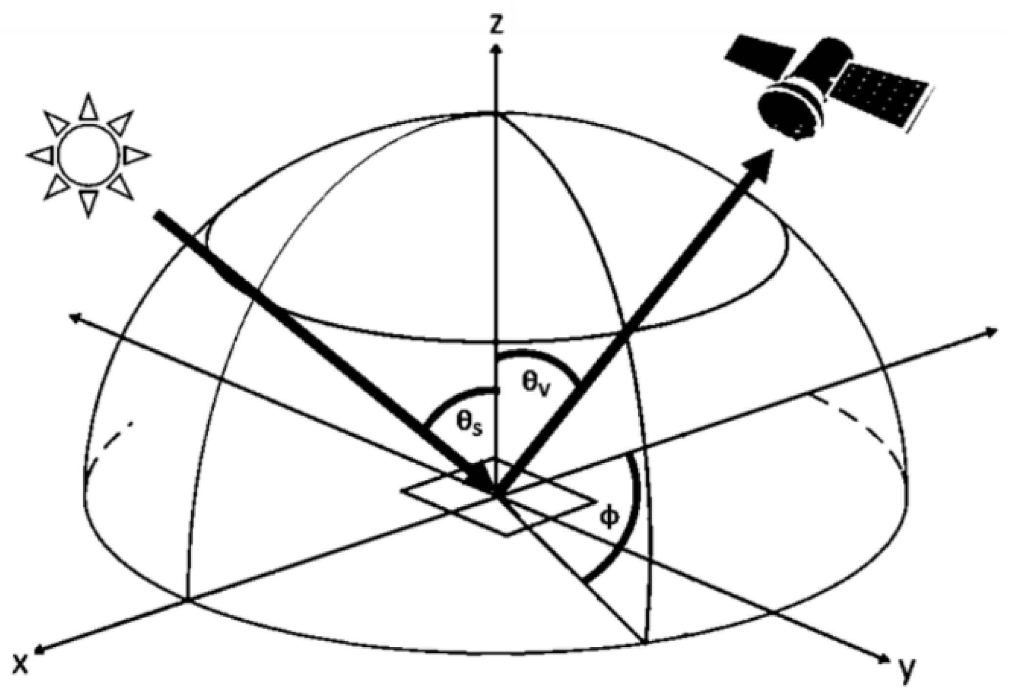
2.1. Anisotropic Factors

ADMs are a set of anisotropic factors that are used to convert observed broadband radiances [W m⁻² sr⁻¹] to irradiances [W m⁻²]. Radiance (L) is the direct measurement for the scanning radiometers common to CERES and Libera, but irradiance (F) is the energetically relevant quantity of interest for virtually all ERB applications. The general relationship between L and F is given by

$$F\left({\theta }_s\right)={\int }_0^{2\pi }{\int }_0^{\pi /2}L\left({\theta }_s, {\theta }_v,\phi \right) cos\left({\theta }_v\right)sin\left({\theta }_v\right)d{\theta }_{v}d\phi ,$$

(1)

where the solar zenith angle, ${\theta }_s$, the viewing zenith angle, ${\theta }_v$, and the relative azimuth angle, $\phi$, show the dependence on the solar-viewing geometry (Figure 1). If the radiances are independent of view direction, i.e., isotropic, the relationship given in Equation (1) reduces to the following:

$$F\left({\theta }_s\right)={\pi L}_{iso}\left({\theta }_s\right).$$

(2)

More generally,

$$F\left({\theta }_S\right)={\displaystyle \frac{\pi L({\theta }_s, {\theta }_v,\phi )}{R({\theta }_s, {\theta }_v,\phi )}},$$

(3)

where R is an anisotropic factor that represents how much the radiance at a given solar-viewing geometry deviates from the isotropic case. It is important to note that both the anisotropic factor, R, and radiance, L, are dependent on ${\theta }_s$, ${\theta }_v$, and $\phi$, whereas the irradiance, F, depends only on ${\theta }_s$.

Figure 1. The relationship between ${\theta }_s$, the solar zenith angle; ${\theta }_v$, the viewing zenith angle; and $\phi$, the relative azimuth angle [12]. The relative azimuth angle is defined from 0 to 180° and is assumed to be azimuthally symmetric from 180 to 360°. The x- and y-axes extend in both directions to span the full horizontal plane, while the z-axis extends only in the positive direction, consistent with the upward-facing hemisphere relevant to the angular sampling of reflected terrestrial radiance.

Figure 1. The relationship between ${\theta }_s$, the solar zenith angle; ${\theta }_v$, the viewing zenith angle; and $\phi$, the relative azimuth angle [12]. The relative azimuth angle is defined from 0 to 180° and is assumed to be azimuthally symmetric from 180 to 360°. The x- and y-axes extend in both directions to span the full horizontal plane, while the z-axis extends only in the positive direction, consistent with the upward-facing hemisphere relevant to the angular sampling of reflected terrestrial radiance.

Anisotropic factors are constructed for each scene and solar-viewing geometry angle bin, where a scene is defined by the underlying surface type and properties of the atmosphere in view of the scanning instrument, as described in the following sections. The construction of empirical anisotropic factors is shown in Equation (4), where $\overline{L_j}$ is the mean radiance for scene j and the set of angular bins, ${\theta }_{s,i}$, ${\theta }_{v,k}$, ${\phi }_l$, while $F_j$ is the upwelling irradiance for scene j and angular bin ${\theta }_{s,i}$,

$$R_j\left({\theta }_{s,i}, {\theta }_{v,k}, {\phi }_l\right)={\displaystyle \frac{\pi \overline{L_j}({\theta }_{s,i},{\theta }_{v,k},{\phi }_l)}{F_j({\theta }_{s.i})}}.$$

(4)

Equation (4) requires an estimation of $F_j\left({\theta }_{s,i}\right)$, which can be accomplished using Equation (5), as described in Loeb et al. (2003) [8]:

$$F_j\left({\theta }_{s,i}\right)={\displaystyle \sum _{l=1}^{l=N_l}}{w}_l{\displaystyle \sum _{k=1}^{N_k}}{w}_k\overline{L_j}({\theta }_{s,i},{\theta }_{v,k},{\phi }_l)\mathit{cos}{\theta }_{v,k},$$

(5)

where $w_l$ and $w_k$ are the Gaussian quadrature weights, and $N_l$ and $N_k$ are the number of Gaussian quadrature points used in the integration. For this calculation to be accurate, the directionally dependent radiance field $\overline{L_j}({\theta }_{s,i},{\theta }_{v,k},{\phi }_l)$ must be sufficiently populated with observations across the relevant ${\theta }_{v,k}$ and ${\phi }_l$ angles. This coverage is typically achieved through RAPS mode observations. The need to ensure adequate sampling of this angular space motivates the analysis in later sections, where we investigate how different RAPS parameters, such as azimuthal scan rate and temporal cadence, affect the density and distribution of scene-angle observations.

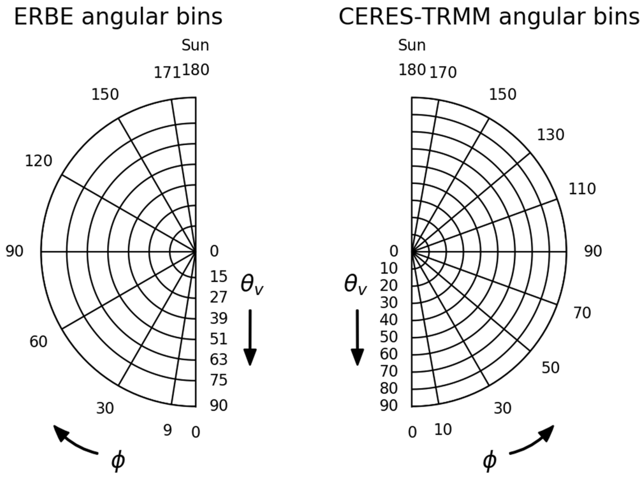
2.2. Scene and Angular Stratification

The number of scene types and angular bins considered when generating ADMs with Equation (4) has varied throughout the ERB satellite data record. For the Earth Radiation Budget Experiment (ERBE) [13], the scene type depended only on the underlying surface type and the cloud fraction [14]. The relative simplicity of the ERBE scene stratification means these scene types can typically be inferred without relying on detailed scene retrieval information from a co-flying imaging instrument such as the Moderate Resolution Imaging Spectroradiometer (MODIS) or the Visible Infrared Imaging Radiometer Suite (VIIRS) [15]. As such, Libera plans to explore the development of ADMs with “ERBE-like” scene types. The exact scene definitions for Libera’s data processing are still under consideration, but for the purposes of this study, we define eleven ERBE-like scene types as listed in

Table 1. ERBE-like shortwave ADM scene types.

Scene ID Number	Cloud Fraction	Surface Type
1	Cloud Free (0–5%)	Ocean
2	Cloud Free (0–5%)	Snow
3	Cloud Free (0–5%)	Land
4	Cloud Free (0–5%)	Desert
5	Partly Cloudy (5–50%)	Ocean
6	Partly Cloudy (5–50%)	Snow
7	Partly Cloudy (5–50%)	Land or Desert
8	Mostly Cloudy (50–95%)	Ocean
9	Mostly Cloudy (50–95%)	Snow
10	Mostly Cloudy (50–95%)	Land or Desert
11	Overcast (95–100%)	All *

* overcast scenes are independent of surface type.

.

The surface types in Table 1 are defined by mapping the latitude and longitude of an observation to the International Geosphere-Biosphere Programme (IGBP) surface type map [16]. The mapping between IGBP, ERBE-like, and TRMM-like surface types is given in

Table 2. International Geosphere-Biosphere Programme surface types.

IGBP Surface Type	ERBE-Like Surface Definition	TRMM-Like Surface Definition
Evergreen Needleleaf Forest	Land	Moderate-to-High Trees/Shrubs
Evergreen Broadleaf Forest	Land	Moderate-to-High Trees/Shrubs
Deciduous Needleleaf Forest	Land	Moderate-to-High Trees/Shrubs
Deciduous Broadleaf Forest	Land	Moderate-to-High Trees/Shrubs
Mixed Forest	Land	Moderate-to-High Trees/Shrubs
Closed Shrublands	Land	Moderate-to-High Trees/Shrubs
Open Shrublands	Desert	Dark Desert
Woody Savannas	Land	Moderate-to-High Trees/Shrubs
Savannas	Land	Low-to-Moderate Trees/Shrubs
Grasslands	Land	Low-to-Moderate Trees/Shrubs
Permanent Wetlands	Land	Low-to-Moderate Trees/Shrubs
Croplands	Land	Low-to-Moderate Trees/Shrubs
Urban and Built-up	Land	Low-to-Moderate Trees/Shrubs
Cropland and Mosaics	Land	Low-to-Moderate Trees/Shrubs
Snow and Ice (permanent)	Snow	Snow
Bare Soil and Rocks	Desert	Bright Desert
Water Bodies	Ocean	Ocean
Tundra	Land	Low-to-Moderate Trees/Shrubs
Fresh Snow	Snow	Snow
Sea Ice	Snow	Snow

.

If a co-flying imager is available, further refined scene stratification is possible. Since Libera is due to co-fly with VIIRS, Libera is also planning to develop ADMs that utilize this information. An initial goal is the scene stratification from the ADMs developed from the CERES instrument that flew on the Tropical Rainfall Measuring Mission (TRMM) satellite [8]. Compared to the ERBE scene types, these scene types are associated with more refined surface types (Table 2), finer binning of cloud fraction, and additional scene properties, including cloud thermodynamic phase and cloud optical depth, as well as surface windspeed for clear-sky ocean scenes. Given these added dimensions and more refined binning, there are over an order of magnitude more TRMM scene types than ERBE ones. There are 591 original TRMM scene types. The first 14 represent cloud-free conditions. The next 336 correspond to ocean or water body surfaces under a range of atmospheric properties. Following these are four land surface types—dark desert, bright desert, low-to-moderate vegetation (trees and shrubs), and moderate-to-high vegetation—each with 60 scene types to represent varying atmospheric conditions. Finally, a single theoretical scene type is used to represent snow-covered surfaces. Loeb et al. (2003) [8] describes the TRMM scene types and the development of the corresponding ADMs. It should be noted that the TRMM scene stratification is still much coarser than that of the latest CERES ADMs [17], which is only possible because of the multiple years of angular sampling acquired by CERES. Given that Libera will initiate the sampling for the broadband split-shortwave channel without any prior or heritage angular observations, we limit the extent of scene stratifications to the TRMM definitions for this study.

For stratification of the angular space, we use the angular bin widths defined for the CERES-TRMM ADMs. While the original ERBE ADMs had slightly coarser angular bins, the differences are not nearly as substantial as those in scene stratification, so we opt to use the CERES-TRMM angular bins for all scene types throughout this study for simplicity. Both the ERBE and TRMM angular bin widths are depicted in Figure 2.

3. Data

The data for this analysis comes from the CERES data record, specifically the Level-2 Single Scanner Footprint (SSF) data product collected during periods when CERES instruments operated in RAPS mode aboard the Suomi National Polar-orbiting Partnership (Suomi-NPP) and Aqua satellites. The Suomi-NPP dataset was selected for this analysis because (i) the CERES instrument on that platform, Flight Model 5 (FM5), was in RAPS from October 2019 to October 2023, and (ii) Suomi-NPP orbits at approximately 824 km altitude [18] with a 98.7° inclination [19], closely matching the planned 833 km altitude and 98.7° inclination of NOAA’s Joint Polar Satellite System-4 (JPSS-4), which will host Libera. This CERES FM5 dataset is utilized in all three analyses presented in Section 5. The Aqua dataset, CERES Flight Model 3 (FM3), was selected for its slower RAPS scan rate of approximately 0.5° per second, compared to approximately 6.5° per second for Suomi-NPP, and is used exclusively in the analysis presented in Section 5.2, which addresses the effect of the RAPS scan rate on the observed angular space. Both Suomi-NPP and Aqua fly in near-polar, sun-synchronous orbits, providing global coverage, including high-latitude and polar regions.

For this study, we analyzed a year’s worth of CERES Suomi-NPP and Aqua data spanning a period from 1 October 2019 to 30 September 2020, resulting in approximately 412 million CERES FM5 footprints from Suomi-NPP and 39 million CERES FM3 footprints from Aqua. The order of magnitude difference between the number of observations analyzed for these two instruments is explained by the Aqua dataset only being utilized in the analysis presented in Section 5.2, which analyzes a 10-day cadence; therefore, only every 10th day of CERES FM3 data from the Aqua satellite was utilized.

Both SSF datasets underwent the same quality control and filtering procedures. Observations flagged for geolocation or radiometric issues were removed, as were those lacking sufficient cloud information. Finally, only footprints occurring on the sunlit side of the orbit (based on solar zenith angle) were retained. Depending on the analysis objectives, several temporal cadences were applied to the FM5 data, including daily, 2-day, 5-day, 10-day, and monthly intervals. These cadences are used consistently throughout Section 5 and are explicitly noted where relevant.

The level-2 SSF data product includes surface, cloud, and aerosol information retrieved from VIIRS on Suomi-NPP [19] and MODIS on Aqua [20]. This provides the information necessary for scene identification for each CERES radiometer footprint. Each single scanner footprint has a resolution of about 20 km and contains up to two cloud layers. For each cloud layer, the cloud amount, optical depth, and phase (liquid or ice) are reported, and these parameters are used in defining TRMM angular distribution model (ADM) scene types. In addition to cloud information, each footprint also has information from the observations made by the CERES radiometers, including filtered total, shortwave, and window radiances for each of the respective channels, as well as the unfiltered shortwave, longwave, and window radiances. The solar-viewing geometry and time are included for each footprint and are used for this analysis.

Although Libera introduces a new split-shortwave spectral channel (0.7 to 5 μm), the Suomi-NPP dataset remains highly suitable for this study. The distribution of surface types and solar zenith angles is primarily governed by orbital parameters rather than spectral response. Since Suomi-NPP and JPSS-4 share key orbital characteristics, including near-identical altitude (824 km vs. 833 km) and inclination (98.7°) values and a 13:30 ascending equatorial crossing time, they offer nearly identical spatial and angular coverage [19]. Therefore, observations from CERES FM5 on Suomi-NPP provide a valid proxy for the types of surface and incident solar radiation conditions that Libera will encounter. This motivates the use of Suomi-NPP RAPS data to assess angular sampling strategies applicable to Libera’s operational context. Of course, due to differences in the spectral response of the shortwave and split-shortwave channels, new split-shortwave ADMs will still be needed to support split-shortwave radiance to irradiance conversions.

4. Methodology

While analyzing the spatial distribution of observations could be useful in broader ERB studies, the ADMs developed for ERBE and TRMM and followed in this study are applied globally for each defined scene type. That is, a single ADM is used for all observations matching a particular surface–atmosphere classification, regardless of their geographic location or season. The utilization of uniform ADMs across seasons and regions is supported by prior research: Loeb et al. (2005) [21] and Su et al. (2015) [17] demonstrate that ADMs can be empirically derived from global CERES-MODIS datasets without seasonal, geographic, or interannual segmentation. As a result, this analysis focuses on sampling coverage across the angular–scene space, without evaluating spatial or interannual variability. Recent studies have shown how regional aerosol loading and properties affect the outgoing radiation field [22,23]; however, the relatively simple ERBE and TRMM ADMs do not consider or incorporate aerosol properties within their scene type definitions. The global, scene-based ADM framework is well established due to its use in prior missions, and it remains consistent with legacy methodologies.

Additionally, this study utilizes one full year of observations. This decision ensures a full annual cycle is captured and also aligns with the operation plans for the Libera mission, which includes RAPS observations in the first year of the mission, provided that a CERES instrument remains active in orbit.

4.1. Methodology for the Impact of RAPS Cadence on Observed Space

An initial assessment of the scene and angular sampling is performed by evaluating how much of the total scene and angular space is observed within a given time frame. To quantify this, the analysis gauges whether a threshold number of observations (or “counts”) under various scenarios is achieved. We focus on the 1-count and 8-count levels. The 1-count level requires that at least a single observation be present in each bin to be considered as filled, while the 8-count level requires at least eight observations to be present in each bin. The 1-count level was selected as it is the most basic count-based quantity to test; it shows whether observations are present at all within a given bin. The 8-count level was chosen as it was the baseline used for the ERBE ADMs, with a bin with fewer than eight samples being treated as missing [14].

It should be noted that while these metrics are consistent with those applied in prior ERB experiments, their direct applicability to Libera’s split-shortwave channel is not presumed. Rather, they provide a simplified baseline measure of angular and scene space coverage. This baseline analysis is further supported by a radiance convergence-based analysis (Section 5.3), which is necessary to quantitatively determine the number of observations, or, more precisely, the number of days of observations, required to obtain a more representative mean radiance for a given scene and angular bin. This, in turn, leads to more accurate anisotropic factors and thus more reliable radiance to irradiance conversions.

In Section 5.1, we apply these count-based metrics to CERES RAPS data from Suomi-NPP to assess how different RAPS cadences affect scene and angular sampling. Two RAPS cadences were tested in this analysis: a monthly cadence, which utilizes a full day of RAPS observations on the first day of each month for a year, and a 10-day cadence, composed of a full day of RAPS observations every 10 days for a year. This comparison was guided by Libera’s azimuthal motor design; the 10-day cadence was selected for testing as it reaches the 50% lifetime limit (with margin) on the azimuthal motor over the five-year prime mission. The monthly cadence provides roughly a factor of three less than the 10-day cadence, and both cadences avoid ground sample aliasing from the 16-day orbit repeat cycle.

4.2. Methodology for Rotational Azimuth Plane Scan (RAPS) Rate Analysis

In Section 5.2, count-based metrics are used to determine how the azimuthal scan rate of the instruments affects the observed angular–scene space. To achieve this, we compare CERES onboard Suomi-NPP, which has an azimuthal scan rate of around 6.5° per second, with CERES onboard Aqua, which has an azimuthal scan rate of approximately 0.5° per second. Intuitively, one might expect the faster azimuthal scan rate to allow Libera’s instrument to observe a larger portion of the scene-type space compared to the slower scan rate, given the same amount of observational time. However, at the faster scan rate of 6.5° per second, the azimuthal motor reaches its lifetime limit more quickly, potentially limiting RAPS scans later in the mission. Much more flexibility will be afforded if Libera scans at the slower rate of 0.5° per second. Importantly, the two datasets have sample sizes of comparable magnitude, approximately 41 million CERES SSF footprints for Suomi-NPP and 39 million for Aqua, allowing for a fair and unbiased comparison of angular–scene coverage.

4.3. Methodology for Bin-by-Bin Radiance Convergence-Based Analysis

Finally, we perform a convergence-based analysis to determine how many observations within a given bin are sufficient for the radiance to converge towards an expected or steady mean value. Analysis of radiance convergence helps determine the number of observations needed to develop accurate ADMs. Specifically, we consider the number of days of observations necessary for the daily mean radiances for a given scene and viewing geometry bin to converge to an expected radiance value. We obtain a mean radiance value for a given scene and angular bin by averaging over daily mean values in an effort to avoid multiple non-independent contributions [8]. Radiance convergence is assessed using CERES SW radiances. It is implicitly assumed that Libera split-SW radiances will exhibit similar behavior, which is a reasonable assumption given that the split-SW bands are spectral subsets of the CERES SW band. We use a full year of Suomi-NPP RAPS observations starting 1 October 2019 to 30 September 2020. This dataset contains roughly 412 million individual CERES footprints, each with an approximate spatial resolution of 20 km. All observations are binned into the TRMM scene and viewing geometry bins. The number of observations per scene and angular bin varies greatly from scene to scene, depending on how frequently that scene occurs naturally, as discussed in Section 5.3. The binned radiances for each scene and viewing geometry bin are then processed into daily mean radiances. The radiance value to which convergence is being assessed is the average of all the daily mean radiances for an entire year for each scene and angular bin:

$$\overline{L_{all, j}}\left({\theta }_{s,i},{\theta }_{v,k},{\phi }_l\right)={\displaystyle \frac{{\sum }_{n=1}^{n=N}{L}_{n,j}\left({\theta }_{s,i},{\theta }_{v,k},{\phi }_l\right)}{N}},$$

(6)

where $L_{n,j}$ is the daily mean radiance for day $n$, scene $j$, and the set of angular bins, ${\theta }_{s,i}$, ${\theta }_{v,k}$, ${\phi }_l$; N is the number of days where there is at least one observation present for the given scene and angular bin, such that N = 365 if there is an observation for each day within the year; and $\overline{L_{all, j}}$ is the average daily mean radiance for all days within a year for the same scene and the set of angular bins.

The convergence towards $\overline{L_{all, j}}$ is considered using three RAPS cadence datasets: a full day of RAPS observations every 10 days, every 5 days, and every 2 days for a year. As discussed in Section 4.1, the 10-day RAPS cadence was selected to avoid aliasing associated with the 16-day orbit repeat cycle, providing a baseline level of angular sampling across the TRMM scene and solar-viewing conditions. The analysis presented in Section 5.1 indicates that while this cadence generally meets minimum sampling requirements, increased RAPS frequencies may offer improved coverage of the TRMM angular–scene space. Therefore, 5-day and 2-day cadences were included to explore the potential benefits of denser sampling and improved radiance convergence within scene and angular bins.

Each dataset contains daily mean radiances binned in the same manner as the dataset to which they are to be compared, that is, by the TRMM scene type and viewing geometry. A Monte Carlo-style approach is applied to each cadence by randomizing the order of daily mean radiances within each bin. To capture variability in the convergence behavior, this randomization process is repeated 80 times. This number was selected based on the physical memory limitations of the computing environment, which constrained the number of complete randomized sequences that could be stored and processed simultaneously. In each case, the full dataset is retained—no observations are omitted or duplicated—and only the order of entries is shuffled. The random permutations are generated using a pseudo-random algorithm designed to produce statistically independent and identically distributed (i.i.d.) sequences, satisfying standard tests of randomness and meeting the conditions required for unbiased convergence analysis. This enables evaluation of the variability and stability of the convergence process by accounting for the effects of random sampling while minimizing biases caused by the sequence of observations. The average daily mean radiance for the first n days for each of the m randomizations is determined using Equation (7), where n is incrementally increased to evaluate the convergence behavior of the mean radiance as a function of the number of days included.

$$\overline{L_{m,n,j}}\left({\theta }_{s,i},{\theta }_{v,k},{\phi }_l\right)={\displaystyle \frac{{\displaystyle {\sum }_1^n}{L}_{m,n,j}\left({\theta }_{s,i},{\theta }_{v,k},{\phi }_l\right)}{n}}.$$

(7)

The absolute difference, $D_{m,n,j}$, for the nth day and mth randomization for each scene and angular bin is as follows:

$$D_{m,n,j}\left({\theta }_{s,i},{\theta }_{v,k},{\phi }_l\right)=\left|\overline{L_{m,n,j}}\left({\theta }_{s,i},{\theta }_{v,k},{\phi }_l\right)-\overline{L_{all, j}}\left({\theta }_{s,i},{\theta }_{v,k},{\phi }_l\right)\right|.$$

(8)

Finally, we take the average across all 80 randomizations, for each scene and viewing geometry bin for each day, n, to calculate a mean absolute difference, $\overline{D_{n,j}}$:

$$\overline{D_{n,j}}({\theta }_{s,i},{\theta }_{v,k},{\phi }_l)={\displaystyle \frac{{\displaystyle {\sum }_1^m}{D}_{m,n,j}({\theta }_{s,i},{\theta }_{v,k},{\phi }_l)}{m}}.$$

(9)

Note that $\overline{D_{n,j}}$ is very similar to the more commonly used mean absolute error. However, $\overline{D_{n,j}}$ is defined as a difference relative to the average daily mean radiance value after a year of observations rather than a known true value. The results of the convergence-based analysis are shown in Section 5.3.

5. Results and Discussion

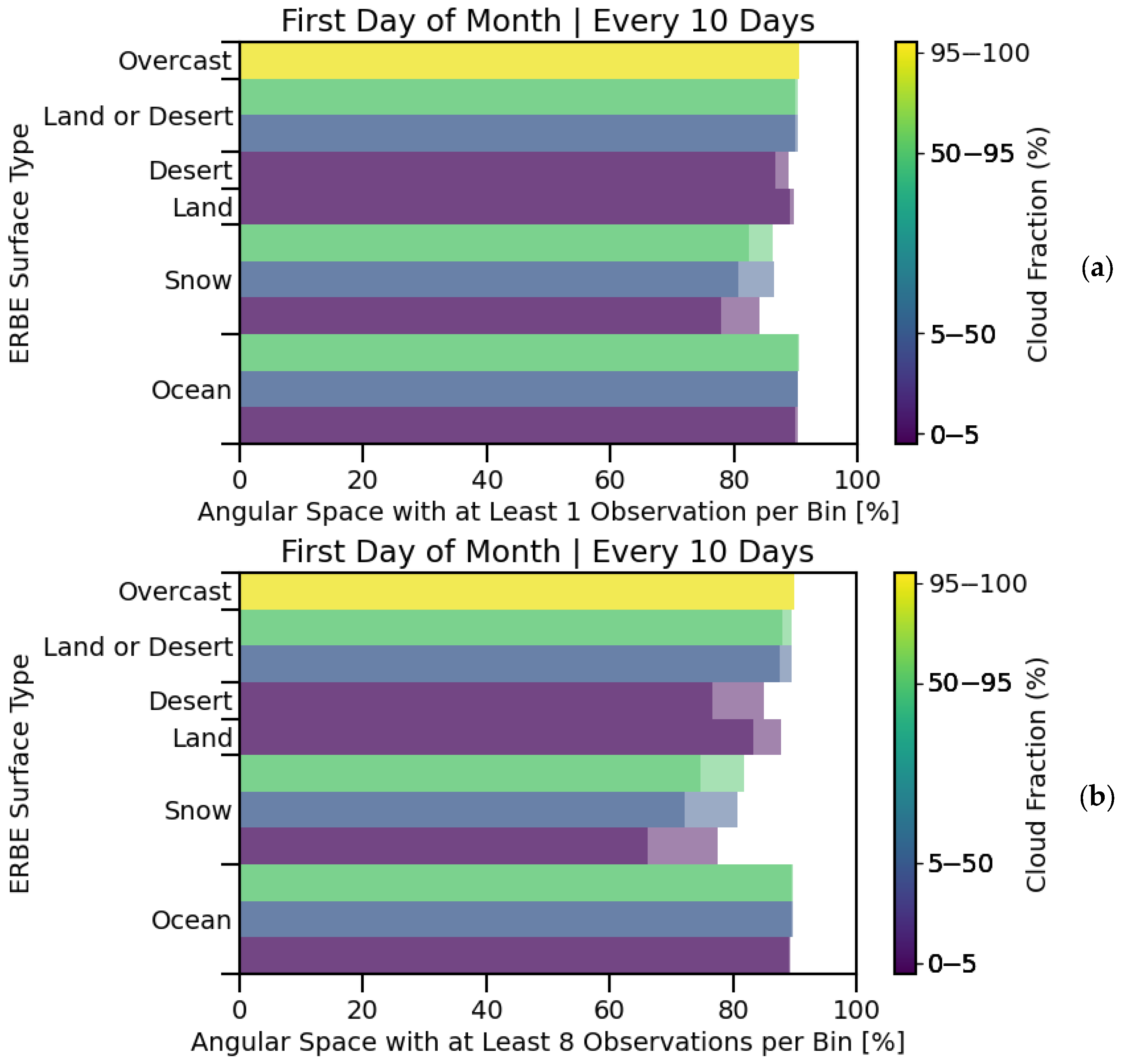
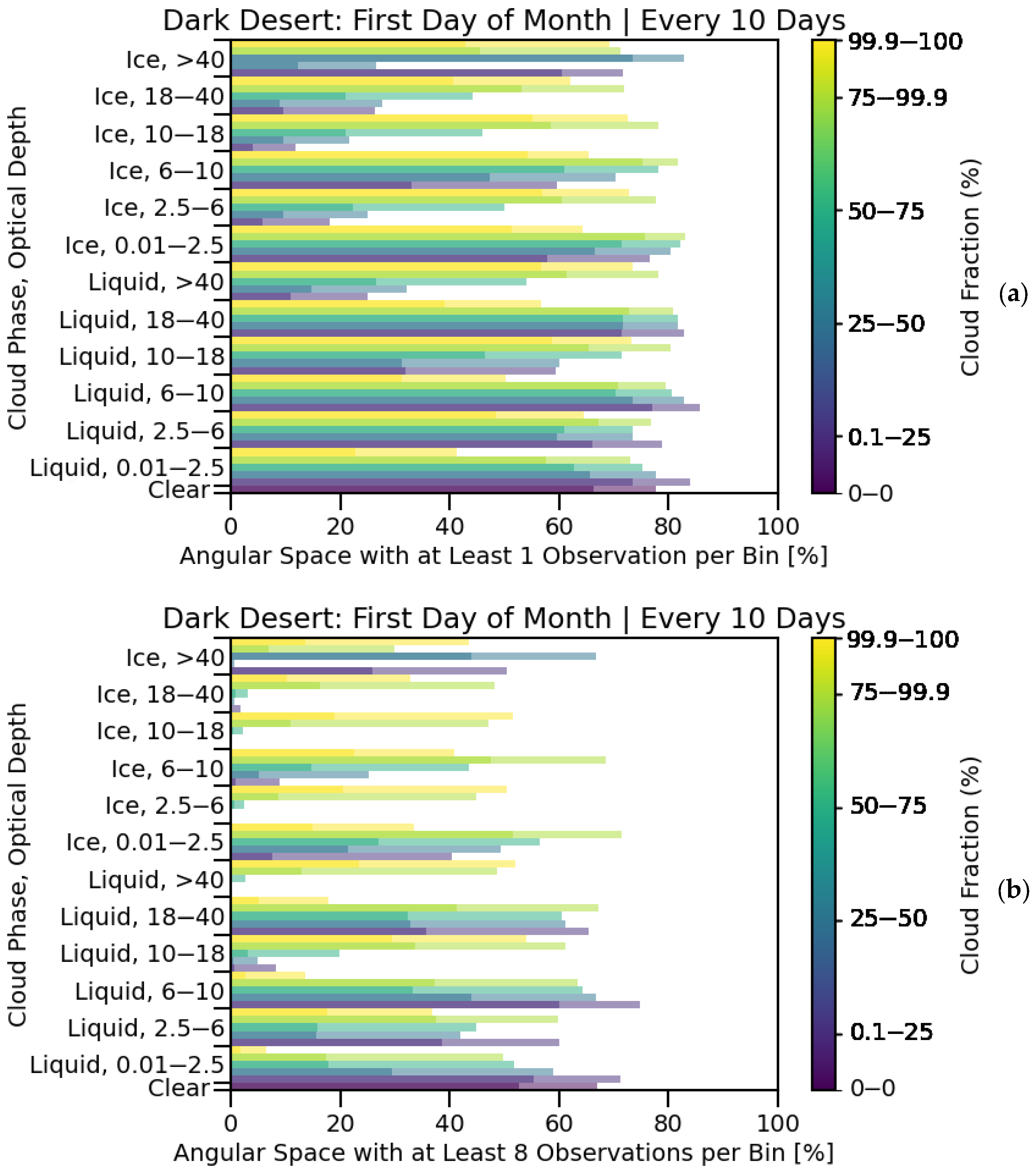
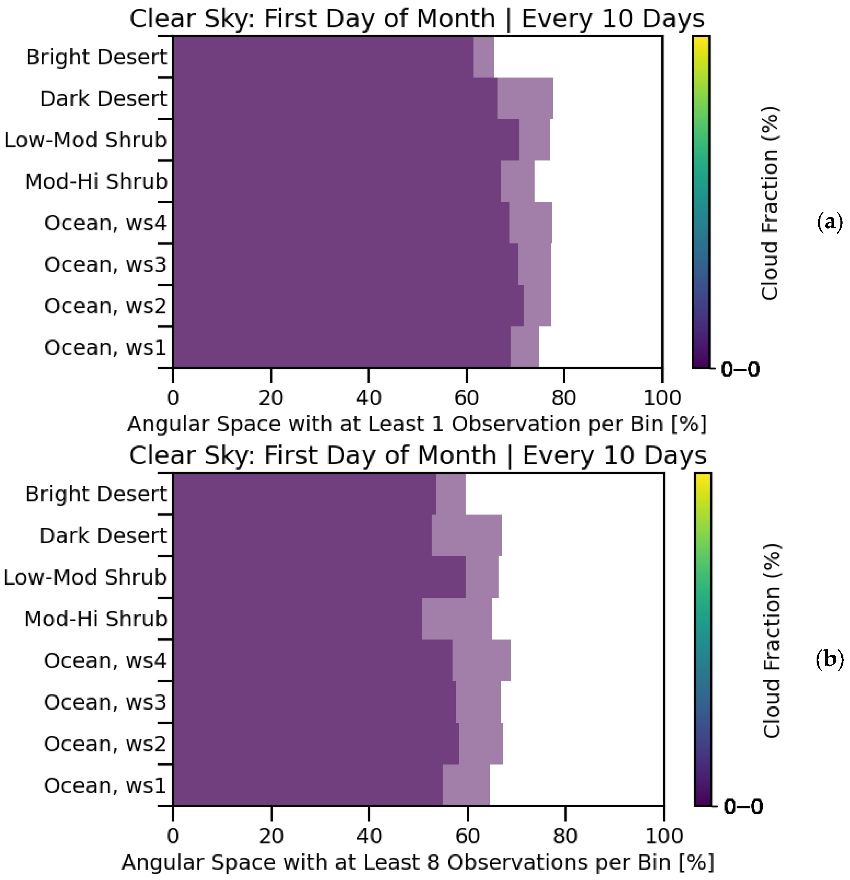
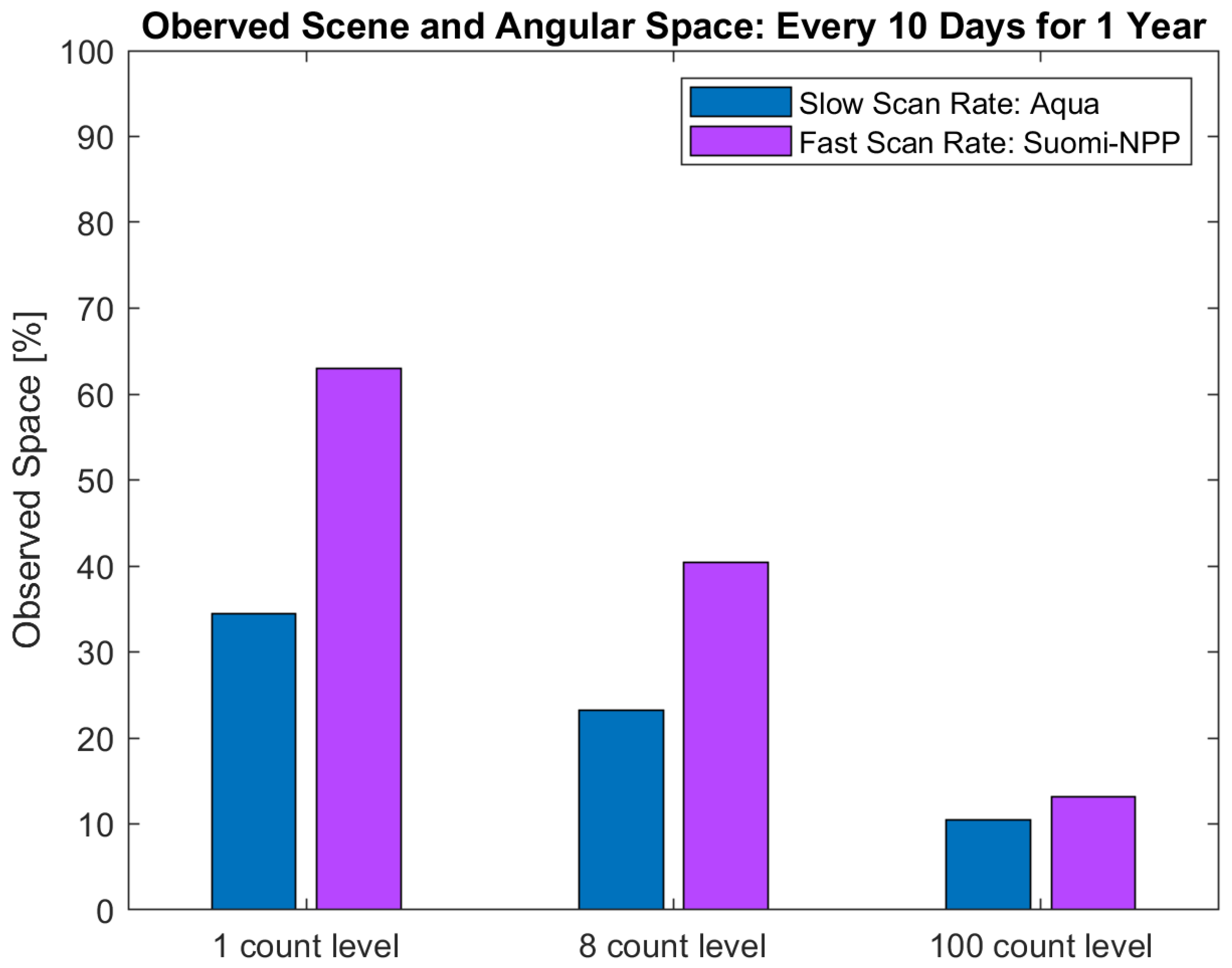
5.1. The Impact of Rotational Azimuth Plane Scan (RAPS) Cadence on Observed Space

This section considers how the RAPS cadence impacts observations of the angular and scene space. Figure 3a shows the observed angular space at the 1-count level for the ERBE scene types, illustrating that there is relatively little improvement when sampling every 10 days over only sampling on the first day of every month. When we inspect the 8-count level (Figure 3b), the largest gain in the observed angular space occurs for scenes with a snowy surface. These scenes have about a 12% gain in the observed angular space when sampling with a 10-day cadence compared to the monthly cadence. It follows that for the more simple ERBE scene types, we can observe most of the angular space, and we obtain only minor improvements when the RAPS scan rate is increased from once a month to every 10 days.

Figure 4a shows the TRMM dark desert surface-type scenes at the 1-count level. It can be seen that a more frequent RAPS cadence is necessary to fill in a similar fraction of the angular space as the number of scene types increases, as is the case when moving from ERBE to TRMM scene types. This is even more apparent when examining the 8 counts per bin level, as shown in Figure 4b. For the monthly RAPS cadence, most of the TRMM dark desert scenes have less than 50% of their solar-viewing geometry filled. The observed angular space roughly doubles when RAPS sampling is increased to the 10-day cadence.

It is not just the added complexity of cloud phase and cloud optical depth within the TRMM scene types that causes this difference in observed angular space, but also the frequency at which certain scenes occur. Simple scene definitions mean that various natural occurrences will satisfy the scene’s requirements. To clarify this, let us consider the difference between the ERBE and TRMM ocean scenes. The ERBE scene types have three ocean scenes: clear sky oceans, partly cloudy oceans, and mostly cloudy oceans, while the TRMM scenes have 346 ocean scenes. Thus, it is obvious why the TRMM scenes need additional RAPS sampling to achieve high angular coverage for all scenes. To further clarify, the CERES-TRMM clear sky scenes, shown in Figure 5 at the 1- and 8-count levels, generally have less viewing geometry space filled with observations than the ERBE counterparts. This can be partly explained when considering how small the first cloud fraction bin is compared to its ERBE equivalent. The TRMM scenes require less than 0.1% of a scene to contain clouds to be classified as a clear sky scene, while the ERBE scene types only require less than 5% to do the same.

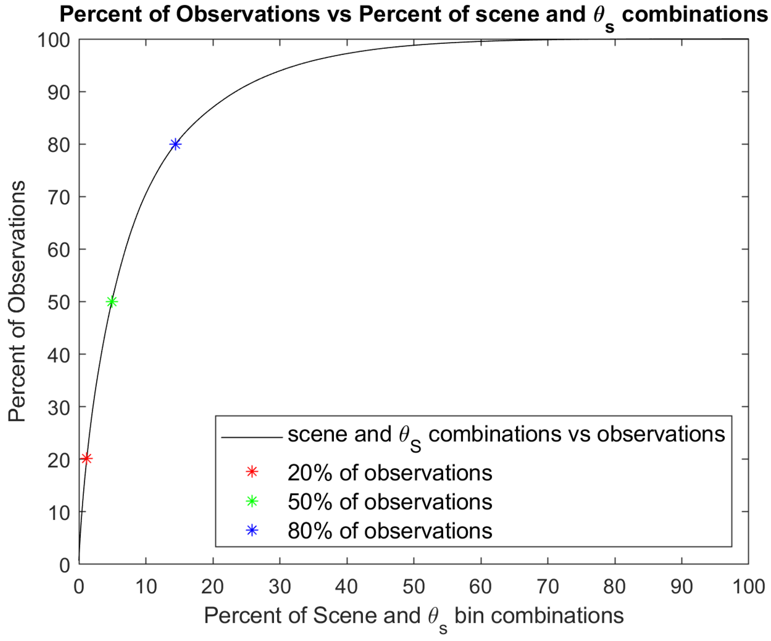
5.2. Rotational Azimuth Plane Scan (RAPS) Rate Analysis

While the previous section quantifies the scene and angular space filled by RAPS for both TRMM and ERBE scenes, an important question still needs to be addressed: how does the azimuthal scan rate of the instruments affect the observed angular–scene space? Figure 6 shows the observed scene and viewing geometry space for the TRMM scenes. At the 1-count level, the fast scan rate observes about 63% of the scene and viewing geometry space, while the slow scan rate observes around 34.5%. At the 8-count level, the difference between the fast and slow scan rates starts to decrease, with the instrument operating in the fast scan rate observing 40.4% of the total scene and viewing geometry space, and the slow scanning instrument filling around 23.3% of the same space. Arbitrarily extending this to the 100-count level shows that the difference between the observed scene and angular space for the slow and fast azimuthal scan rates becomes minimal. At the 100-count level, the fast scan rate observes 13.2% of the space, while the slower RAPS mode (0.5° per second) observes around 10.4% of the same space.

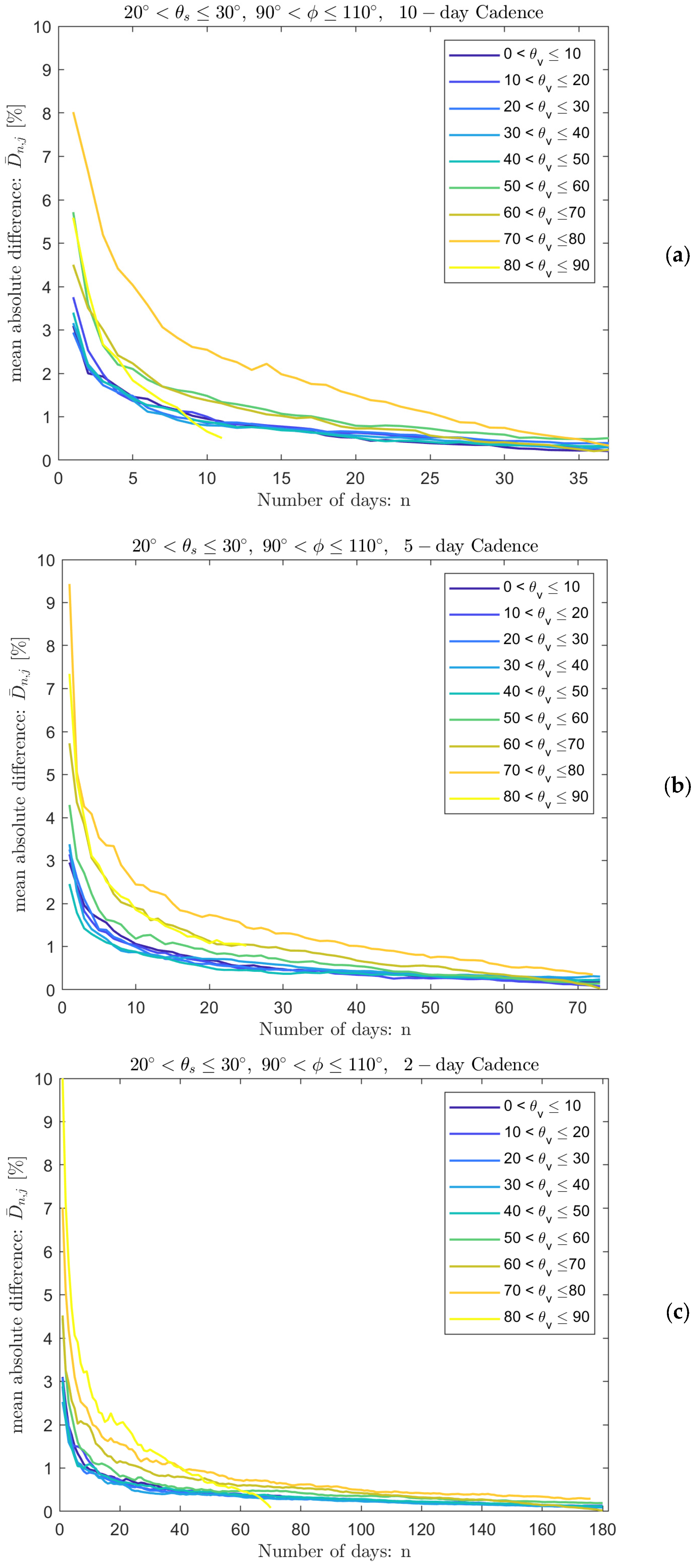
5.3. Bin-by-Bin Radiance Convergence-Based Analysis

The count-based analysis shown in the previous two sub-sections provides a valuable baseline for how much of the scene and angular space of TRMM and ERBE scenes is observed with respect to the number of RAPS days and the scan rate. However, further analysis is needed to test the proficiency of sampling within a given bin. Thus, bin-by-bin radiance convergence-based analysis has been performed. It is important to note that most of the observations from Suomi-NPP fall into a few TRMM scene and ${\theta }_s$ combinations (Figure 7). This figure shows the cumulative distribution function (CDF) of the relative percent of observations as a function of scene and ${\theta }_s$ combination. To generate this CDF, we found the total number of times that each scene–${\theta }_s$ combination was observed over the one-year dataset. We then sorted the scene–${\theta }_s$ combination from most to least frequently observed, based purely on how many observations there were for each combination within the one-year time frame. The x-axis in Figure 7 represents this ordered list of bins (not specific scene types or angles), while the y-axis shows the cumulative percentage of total observations contained in the top x% of bins. The colored stars on the figure show that 20% of all the Suomi-NPP observations fall into only 1.2% of the possible TRMM scene and ${\theta }_s$ combinations, 50% of all the observations are composed of 4.9% scene-${\theta }_s$ combinations, and 80% of all the observations are covered by 14.4% scene-${\theta }_s$ combinations. The green star (50%) indicates the median bin in terms of cumulative observation density, not a specific scene or angle, highlighting how a few combinations dominate the dataset. We will reference the scene-${\theta }_s$ combinations located in the region around the green star as moderately common scene-${\theta }_s$ combinations.

This emergent property of the scene and angular sampling is something that Libera can exploit. If the radiometers can achieve sufficient angular sampling across the ${\theta }_v$ and $\phi$ viewing geometry components for the most commonly occurring scenes and ${\theta }_s$ combinations, the radiometer-based split-shortwave ADMs can support the evaluation of the majority of the radiance to irradiance conversions that Libera will make. In doing so, a limited set of radiometer-derived ADMs play a critical role in anchoring the new WFOV camera-based ADM framework with established methods.

With the relationship between total observations and scene-${\theta }_s$ combinations in mind, Figure 8 shows the decrease in the mean absolute difference, $\overline{D_{n,j}}$ (Equation (9)), as the number of days (n) increases for the most common TRMM scene and ${\theta }_s$ combination. Each curve represents the relationship for a single ${\theta }_v$ bin. For the 10-day cadence (Figure 8a), the mean absolute difference, $\overline{D_{n,j}}$, for each ${\theta }_v$ bin decreases rapidly at first as the number of days increases from 0, converging towards a mean absolute difference of 0%. By the end of the 10-day cadence, the average $\overline{D_{n,j}}$ across all ${\theta }_v$ bins is 0.34%. A similar trend can be seen for the 5-day (Figure 8b) and 2-day (Figure 8c) cadences. By the end of the 5-day cadence, the average $\overline{D_{n,j}}$ across all ${\theta }_v$ bins is 0.28%, resulting in a 0.06% gain after doubling the number of days of observations. For the 2-day cadence, the average $\overline{D_{n,j}}$ across the nine ${\theta }_v$ bins is 0.13%, yielding a 0.21% gain. Although $\overline{D_{n,j}}$ becomes closer to 0% for the 5-day and 2-day cadences than for the 10-day cadence, the difference is not substantial.

The same is not true when analyzing the scene and ${\theta }_s$ combinations near the green point in Figure 7. We will reference these scenes and ${\theta }_s$ combinations as moderately common combinations. By the end of the 10-day cadence, the average $\overline{D_{n,j}}$ across all ${\theta }_v$ bins is 0.75%. At the end of the 5-day cadence, the average decreases to 0.44%, representing a 0.31% improvement. For the 2-day cadence, the average is 0.27%, yielding a total improvement of 0.48% relative to the 10-day cadence. While $\overline{D_{n,j}}$ decreases rapidly during the first few days for all three cadences, Figure 9 shows a consistent and measurable improvement in convergence behavior when moving from the 10-day (Figure 9a) to either the 5-day (Figure 9b) or 2-day (Figure 9c) cadence. Thus, there may be benefits in considering one of these more frequent RAPS cadences for Libera’s operations within the first year of the mission.

6. Conclusions

Angular distribution models are used to convert observed broadband satellite radiances to the ERB-relevant quantity of irradiance. The development of ADMs has traditionally required an extensive amount of RAPS observations to obtain the necessary radiances across a vast combination of viewing angles and scene types. For the upcoming Libera mission, ADM generation and evaluation is required for the new split-shortwave channel. Yet, there is also a desire to minimize time in RAPS mode for the continuity of the climate data record. Data from a wide-field-of-view camera will assist in generating new ADMs, but this needs to be evaluated with angular sampling from the split-shortwave radiometer itself. Consequently, this study provides an assessment of the angular sampling that Libera can achieve with various RAPS options.

For simple scene type definitions, such as the ERBE scene types, we find that the scene and viewing geometry space would be well sampled with a RAPS cadence of just one day per month during the first year of the Libera mission, observing 87% of the scene and angular space at the 1-count level and 82% at the 8-count level. Increasing the cadence to every 10 days results in a 2% and 5% increase at the 1- and 8-count levels, respectively. However, our analysis also shows that increasing the RAPS cadence from once a month to every 10 days provides a much better sampling of the angular–scene space for the more stratified TRMM scene types within the first year. When increasing the cadence, the TRMM scene types expand from sampling 54% to 66% at the 1-count level and increasing the observed space from 29% to 43% at the 8-count level. This initial analysis only considers the total observation counts within the scenes and angular bins. However, this already indicates that improved sampling would be possible for TRMM scenes with a higher RAPS cadence.

Utilizing two CERES instruments, CERES onboard Suomi-NPP with a relatively fast azimuthal scan rate and CERES onboard Aqua with a relatively slow azimuthal scan rate, our analysis compares the effect of the azimuthal scan rate on the observed TRMM scene and viewing geometry space. Intuitively, a faster scan rate would appear to encompass a larger portion of the scene and viewing geometry space compared to a slower rate, given the same observational time. While this trend is apparent in the analysis above, we demonstrated that for a given amount of azimuthal rotation, a key constraint for the Libera mission, the angular and viewing geometry space of the TRMM scene types is sampled more comprehensively by operating at the slower azimuthal rotation rate for a longer period of time.

A vast majority of the CERES observations on Suomi-NPP fall into just a few TRMM scene and ${\theta }_s$ combinations. For example, 50% of the observations are represented by 4.9% of the scene-${\theta }_s$ combinations. Therefore, it is expected that Libera will be able to develop RAPS-based ADMs for the most frequent scene and ${\theta }_s$ combinations that will be relevant for most observed footprints. For these most common scene and ${\theta }_s$ combinations, a 10-day RAPS cadence results in a difference of half a percent or less compared to the average daily mean radiance for all days within a year. For the moderately common scene-${\theta }_s$ combinations, a substantial improvement occurs when increasing from the 10-day to the 5-day or 2-day cadences. Therefore, this analysis suggests that Libera may benefit from a RAPS cadence of 2–5 days for the first year of operations.

References

1. Coddington, O.M.; Richard, E.C.; Harber, D.; Pilewskie, P.; Woods, T.N.; Chance, K.; Liu, X.; Sun, K. The TSIS-1 Hybrid Solar Reference Spectrum. Geophys. Res. Lett. 2021, 48, e2020GL091709. [Google Scholar] [CrossRef]
2. Wielicki, B.A.; Barkstrom, B.R.; Harrison, E.F.; Lee, R.B.; Smith, G.L.; Cooper, J.E. Clouds and the Earth’s Radiant Energy System (CERES): An Earth Observing System Experiment. Bull. Am. Meteorol. Soc. 1996, 77, 853–868. [Google Scholar] [CrossRef]
3. Loeb, N.G.; Su, W.; Doelling, D.R.; Wong, T.; Minnis, P.; Thomas, S.; Miller, W.F. 5.03—Earth’s Top-of-Atmosphere Radiation Budget. In Comprehensive Remote Sensing; Liang, S., Ed.; Elsevier: Oxford, UK, 2018; pp. 67–84. ISBN 978-0-12-803221-3. [Google Scholar]
4. Loeb, N.G.; Johnson, G.C.; Thorsen, T.J.; Lyman, J.M.; Rose, F.G.; Kato, S. Satellite and Ocean Data Reveal Marked Increase in Earth’s Heating Rate. Geophys. Res. Lett. 2021, 48, e2021GL093047. [Google Scholar] [CrossRef]
5. Nerem, R.S.; Beckley, B.D.; Fasullo, J.T.; Hamlington, B.D.; Masters, D.; Mitchum, G.T. Climate-change–driven accelerated sea-level rise detected in the altimeter era. Proc. Natl. Acad. Sci. USA 2018, 115, 2022–2025. [Google Scholar] [CrossRef]
6. Ebi, K.L.; Vanos, J.; Baldwin, J.W.; Bell, J.E.; Hondula, D.M.; Errett, N.A.; Hayes, K.; Reid, C.E.; Saha, S.; Spector, J.; et al. Extreme Weather and Climate Change: Population Health and Health System Implications. Annu. Rev. Public Health 2021, 42, 293–315. [Google Scholar] [CrossRef] [PubMed]
7. Wong, T.; Smith, G.L.; Kato, S.; Loeb, N.G.; Kopp, G.; Shrestha, A.K. On the Lessons Learned From the Operations of the ERBE Nonscanner Instrument in Space and the Production of the Nonscanner TOA Radiation Budget Data Set. IEEE Trans. Geosci. Remote Sens. 2018, 56, 5936–5947. [Google Scholar] [CrossRef] [PubMed]
8. Loeb, N.G.; Manalo-Smith, N.; Kato, S.; Miller, W.F.; Gupta, S.K.; Minnis, P.; Wielicki, B.A. Angular Distribution Models for Top-of-Atmosphere Radiative Flux Estimation from the Clouds and the Earth’s Radiant Energy System Instrument on the Tropical Rainfall Measuring Mission Satellite. Part I: Methodology. J. Appl. Meteor. 2003, 42, 240–265. [Google Scholar] [CrossRef]
9. Hakuba, M.Z.; Kindel, B.; Gristey, J.; Bodas-Salcedo, A.; Stephens, G.; Pilewskie, P. Simulated Variability in Visible and Near-IR Irradiances in Preparation for the Upcoming Libera Mission; AIP Publishing: Thessaloniki, Greece, 2024; p. 050006. [Google Scholar]
10. Gristey, J.J.; Schmidt, K.S.; Chen, H.; Feldman, D.R.; Kindel, B.C.; Mauss, J.; Van Den Heever, M.; Hakuba, M.Z.; Pilewskie, P. Angular sampling of a monochromatic, wide-field-of-view camera to augment next-generation Earth radiation budget satellite observations. Atmos. Meas. Tech. Discuss. 2023, 16, 3609–3630. [Google Scholar] [CrossRef]
11. Kampe, T.U.; Schmitt, S.; Gristey, J.J.; Harber, D.; Pilewskie, P.; Spuhler, P.; Gordon, M.; Amparan, B.; Bannon, E.; Vujcich, M.; et al. Libera’s wide-field-of-view camera for augmenting next-generation Earth radiation budget satellite observations. In Proceedings of the CubeSats, SmallSats, and Hosted Payloads for Remote Sensing VIII; Pagano, T.S., Puschell, J.J., Babu, S.R., Eds.; SPIE: San Diego, CA, USA, 2024; p. 4. [Google Scholar]
12. Gristey, J.J.; Su, W.; Loeb, N.G.; Vonder Haar, T.H.; Tornow, F.; Schmidt, K.S.; Hakuba, M.Z.; Pilewskie, P.; Russell, J.E. Shortwave Radiance to Irradiance Conversion for Earth Radiation Budget Satellite Observations: A Review. Remote Sens. 2021, 13, 2640. [Google Scholar] [CrossRef]
13. Barkstrom, B.R. The Earth Radiation Budget Experiment (ERBE). Bull. Am. Meteor. Soc. 1984, 65, 1170–1185. [Google Scholar] [CrossRef]
14. Suttles, J.; Green, R.; Minnis, P.; Smith, G.; Staylor, W.; Wielicki, B.; Walker, I.; Young, D.; Taylor, V.; Stowe, L. Angular radiation models for Earth-atmosphere system. NASA Ref. Publ. 1184 1988, 1, 88N27677. [Google Scholar]
15. Smith, G.L.; Green, R.N.; Raschke, E.; Avis, L.M.; Suttles, J.T.; Wielicki, B.A.; Davies, R. Inversion methods for satellite studies of the Earth’s Radiation Budget: Development of algorithms for the ERBE Mission. Rev. Geophys. 1986, 24, 407–421. [Google Scholar] [CrossRef]
16. CERES: IGBP Land Classification. Available online: https://climatedataguide.ucar.edu/climate-data/ceres-igbp-land-classification (accessed on 1 November 2024).
17. Su, W.; Corbett, J.; Eitzen, Z.; Liang, L. Next-generation angular distribution models for top-of-atmosphere radiative flux calculation from CERES instruments: Methodology. Atmos. Meas. Tech. 2015, 8, 611–632. [Google Scholar] [CrossRef]
18. Miller, S.; Straka, W.; Mills, S.; Elvidge, C.; Lee, T.; Solbrig, J.; Walther, A.; Heidinger, A.; Weiss, S. Illuminating the Capabilities of the Suomi National Polar-Orbiting Partnership (NPP) Visible Infrared Imaging Radiometer Suite (VIIRS) Day/Night Band. Remote Sens. 2013, 5, 6717–6766. [Google Scholar] [CrossRef]
19. Wolfe, R.E.; Lin, G.; Nishihama, M.; Tewari, K.P.; Tilton, J.C.; Isaacman, A.R. Suomi NPP VIIRS prelaunch and on-orbit geometric calibration and characterization. J. Geophys. Res. Atmos. 2013, 118, 11508–11521. [Google Scholar] [CrossRef]
20. Scott, R.C.; Rose, F.G.; Stackhouse, P.W.; Loeb, N.G.; Kato, S.; Doelling, D.R.; Rutan, D.A.; Taylor, P.C.; Smith, W.L. Clouds and the Earth’s Radiant Energy System (CERES) Cloud Radiative Swath (CRS) Edition 4 Data Product. J. Atmos. Ocean. Technol. 2022, 39, 1781–1797. [Google Scholar] [CrossRef]
21. Loeb, N.G.; Kato, S.; Loukachine, K.; Manalo-Smith, N. Angular Distribution Models for Top-of-Atmosphere Radiative Flux Estimation from the Clouds and the Earth’s Radiant Energy System Instrument on the Terra Satellite. Part I: Methodology. J. Atmos. Ocean. Technol. 2005, 22, 338–351. [Google Scholar] [CrossRef]
22. Wang, L.; Su, X.; Wang, Y.; Cao, M.; Lang, Q.; Li, H.; Sun, J.; Zhang, M.; Qin, W.; Li, L.; et al. Towards long-term, high-accuracy, and continuous satellite total and fine-mode aerosol records: Enhanced Land General Aerosol (e-LaGA) retrieval algorithm for VIIRS. ISPRS J. Photogramm. Remote Sens. 2024, 214, 261–281. [Google Scholar] [CrossRef]
23. Jin, S.; Ma, Y.; Li, H.; Liu, B.; Fan, R.; Zhang, M.; Lopatin, A.; Dubovik, O.; Hu, X.; Gong, W.; et al. Characterizing Aerosol Optical Properties and Direct Radiative Effects From the Perspective of Components: A Synergy Retrieval Study Based on Sun Photometer and Lidar in Central China. Geophys. Res. Lett. 2025, 52, e2024GL113448. [Google Scholar] [CrossRef]
24. van den Heever, M.; Gristey, J.; Pilewskie, P. Optimizing the Sampling Strategy for Future Libera Earth Radiation Budget Satellite Observations. In Proceedings of the Optimizing the Sampling Strategy for Future Libera Earth Radiation Budget Satellite Observations, Hangzhou, China, 17 June 2024. [Google Scholar]
Figure 2. ERBE (left) and CERES-TRMM (right) shortwave ADM viewing zenith angle ( θ v ) and relative azimuth angle (ϕ) bins [12].
Remotesensing 17 02540 g002
Figure 3. Observed scene and angular space for ERBE scene types. Each bar shows the percent of angular space with at least (a) one observation or (b) eight observations per θ s , θ v , and φ bin combination for an ERBE scene type. The solid portion of each bar represents the amount of each scene type observed for the monthly cadence, while the transparent portion at the end of each bar represents the observed angular space that is gained over the monthly cadence when increasing the RAPS sampling to the 10-day cadence.
Remotesensing 17 02540 g003
Figure 4. The observed angular space at (a) the 1-count level and (b) the 8-count level for each CERES-TRMM Dark Desert scene type. The solid portion of each bar represents the amount of each scene type with at least one (a) or eight (b) observations per bin for the monthly cadence. The transparent portion at the end of each bar represents the amount of angular space gained by switching from a monthly cadence to a 10-day cadence.
Remotesensing 17 02540 g004
Figure 5. The amount of angular space with at least (a) one observation and (b) eight observations per θ s , θ v , and φ bin combination for TRMM’s clear-sky scene types. There are four clear-sky scene types for the ocean surface type, each with a different windspeed (ws). Ws1 has a surface windspeed of less than 3.5 m s−1, ws2 ranges from 3.5 to 5.5 m s−1, ws3 ranges from 5.5 to 7.5 m s−1, and ws4 is greater than 7.5 m s−1. The solid portion of each bar represents the amount of each scene type with at least (a) one observation or (b) eight observations per bin for the monthly cadence. The more transparent portion at the end of each bar represents the amount of angular space gained over the monthly cadence when increasing to the 10-day RAPS cadence.
Remotesensing 17 02540 g005
Figure 6. Observed TRMM scene and angular space for two RAP scan rates with a RAPS cadence of every 10 days for a year. The purple bars show the observed scene and viewing geometry space for the fast scan rate (6.5° per second), derived from CERES onboard Suomi-NPP. The blue bars show the observed scene and viewing geometry space for the slow scan rate (0.5° per second), derived from CERES onboard Aqua.
Remotesensing 17 02540 g006
Figure 7. Cumulative distribution function (CDF) showing the relative amount observations as a function of the number of scene and θ s combinations. We have ordered the scene and θ s combinations from most to least frequent. The CDF illustrates how a relatively small number of scene and θ s combinations account for the majority of observations, providing insight into the representativeness and distribution of scene sampling within the dataset.
Remotesensing 17 02540 g007
Figure 8. D n , j ¯ as a function of the number of days for the most common TRMM scene and θ s combination and a 10-day (a), 5-day (b), and 2-day (c) RAPS cadence. The most common TRMM scene and θ s combination is a liquid cloud over the ocean with a cloud fraction of 0.1 to 10%, an optical depth of 1–2.5, and a solar zenith bin of 20° < θ s < 30°. All possible θ v bins are shown for the relative azimuth bin 90° < φ < 110°.
Remotesensing 17 02540 g008
Figure 9. D n , j ¯ as a function of the number of days for a moderately common TRMM scene and θ s combination and a 10-day (a), 5-day (b), and 2-day (c) RAPS cadence. The following parameters are for a moderately common TRMM scene and θ s combination: a liquid cloud over the ocean with a cloud fraction of 95 to 99.9%, an optical depth of 10–12.5, and a θ s bin of 20°–30°. All possible θ v bins are shown for the φ bin of 90° to 110°.
Remotesensing 17 02540 g009