
A Method for Auto Generating a Remote Sensing Building Detection Sample Dataset Based on OpenStreetMap and Bing Maps

 ,
,
Abstract
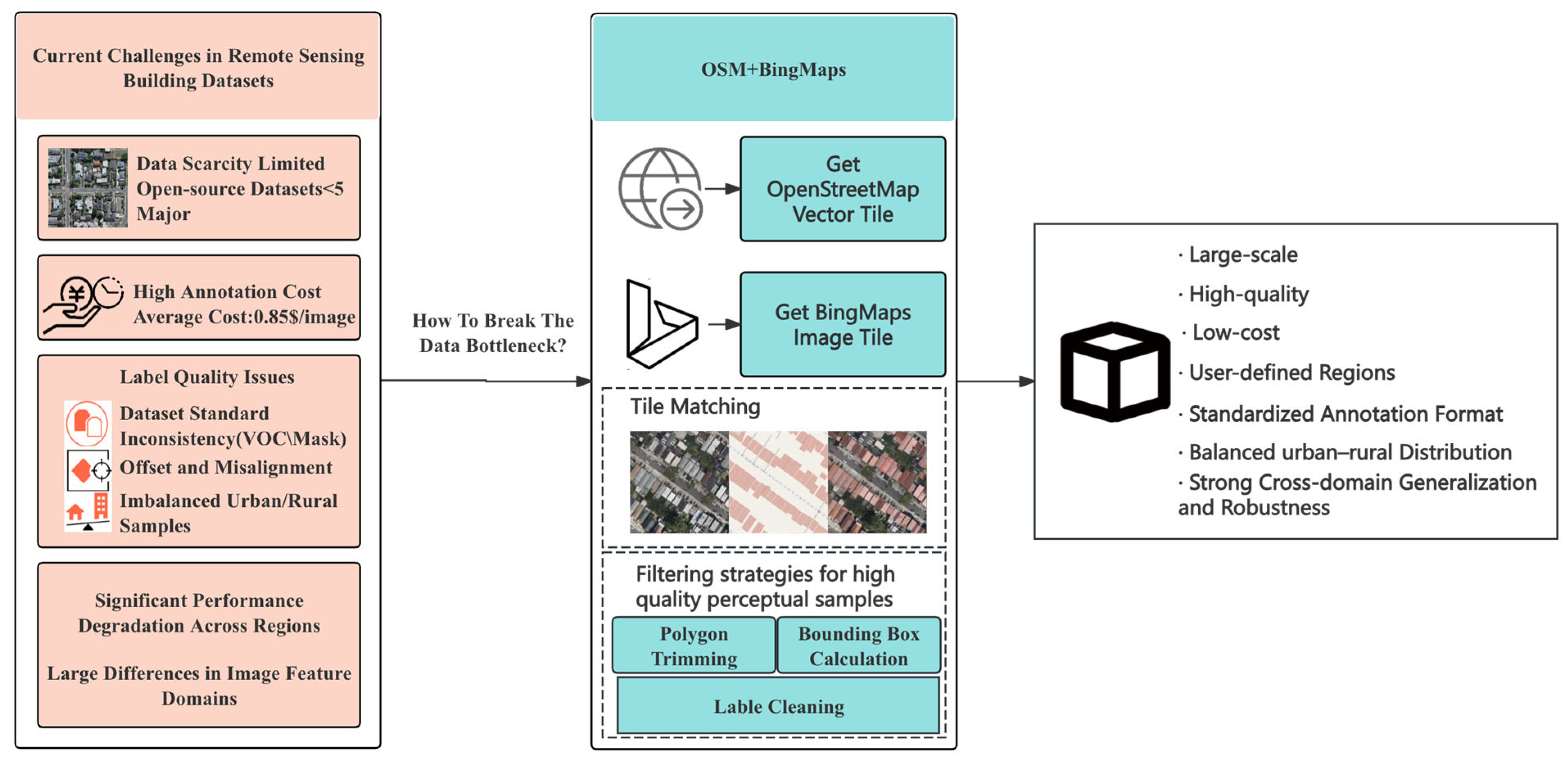
1. Introduction
- We propose a robust and scalable automatic building annotation algorithm named MapAnnoFactory, which leverages geographic vector data from OpenStreetMap. Through projection transformation, it achieves precise alignment with high-resolution satellite imagery from Bing Maps. A quality-aware sample filtering strategy is incorporated to automatically generate high-precision building detection annotations.
- Using MapAnnoFactory we constructed a large-scale building dataset named AutoBuildRS, which contains 36,647 fully annotated samples covering multiple metropolitan areas in Australia and North America.
- Extensive experiments were conducted using four representative object detection models—SSD, Faster R-CNN, DETR, and YOLOv11s—and compared against the following three widely used open-source benchmark datasets: Wuhan University dataset (WHU), Institut National de Recherche en Informatique et en Automatique dataset (INRIA), and Dizhi University dataset (DZU). Evaluation metrics included mean average precision (mAP), precision, recall, and F1-score. Additional tests on input perturbation robustness and cross-dataset generalization further demonstrated the advantages of the proposed dataset in terms of detection accuracy, robustness, and generalization capability. Finally, experiments on a publicly available test region confirmed the outstanding performance and strong cross-regional transferability of the dataset generated by this framework.
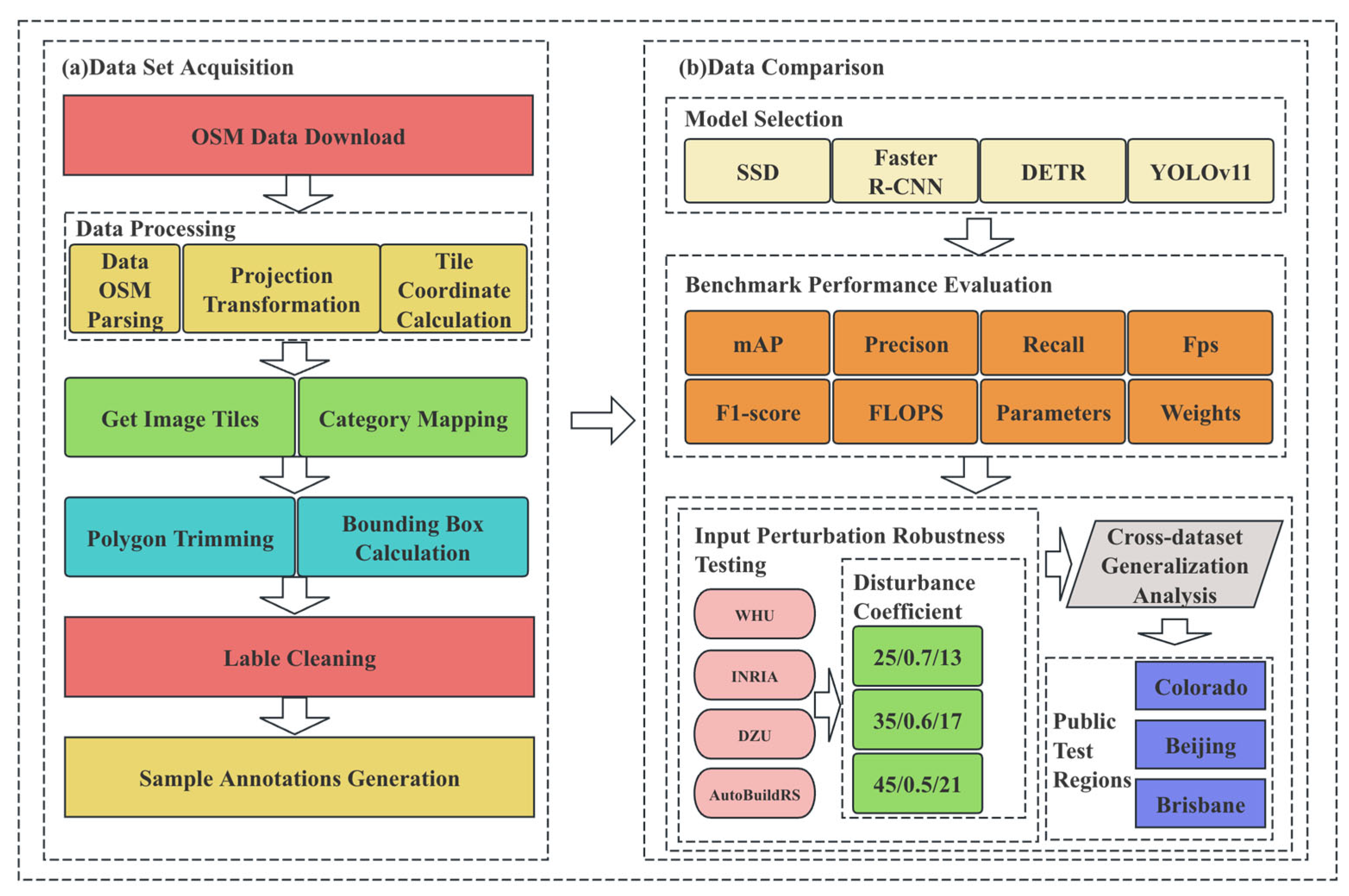
2. Materials and Methods
2.1. Materials
2.1.1. Open-Source Datasets
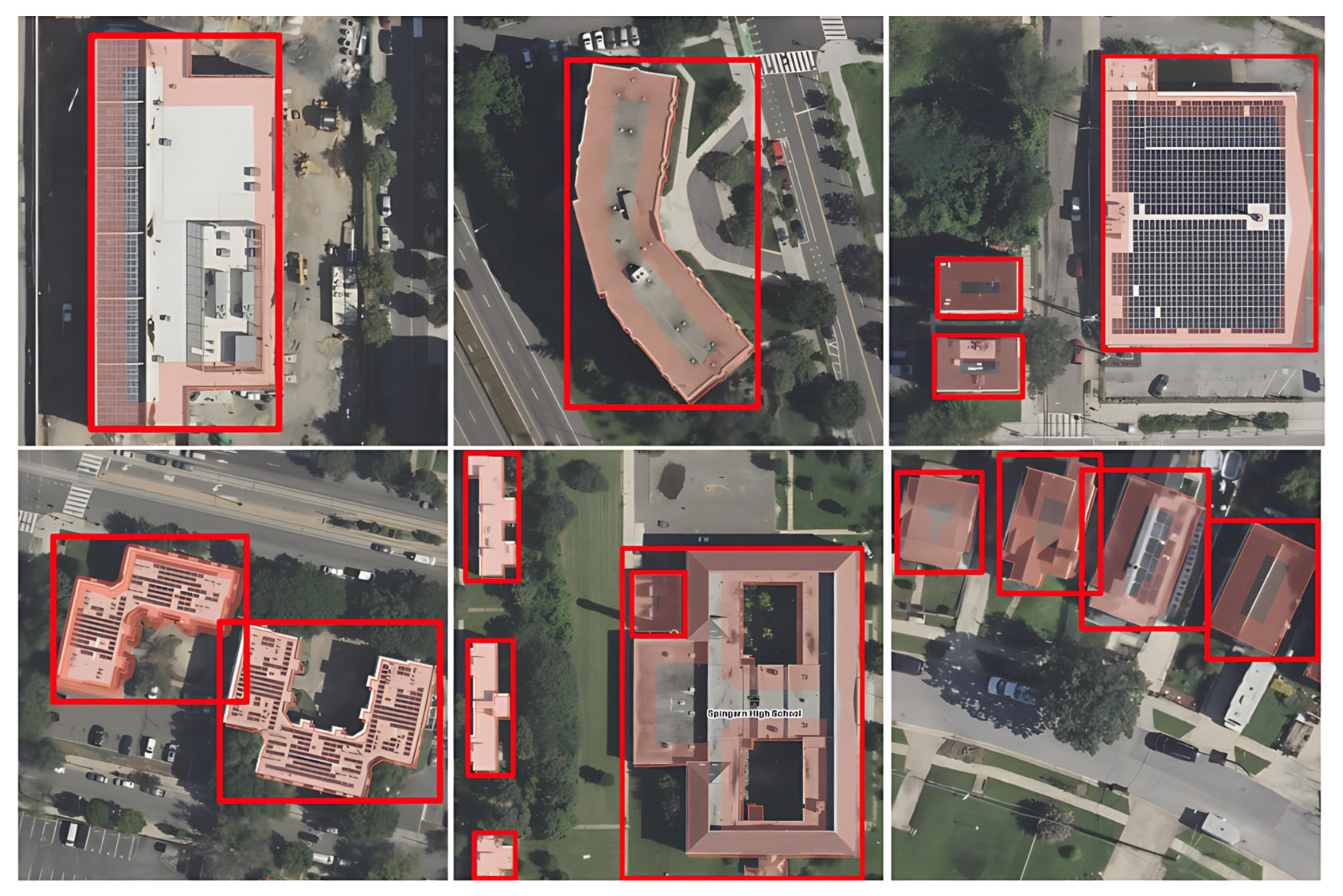
2.1.2. AutoBuildRS Dataset
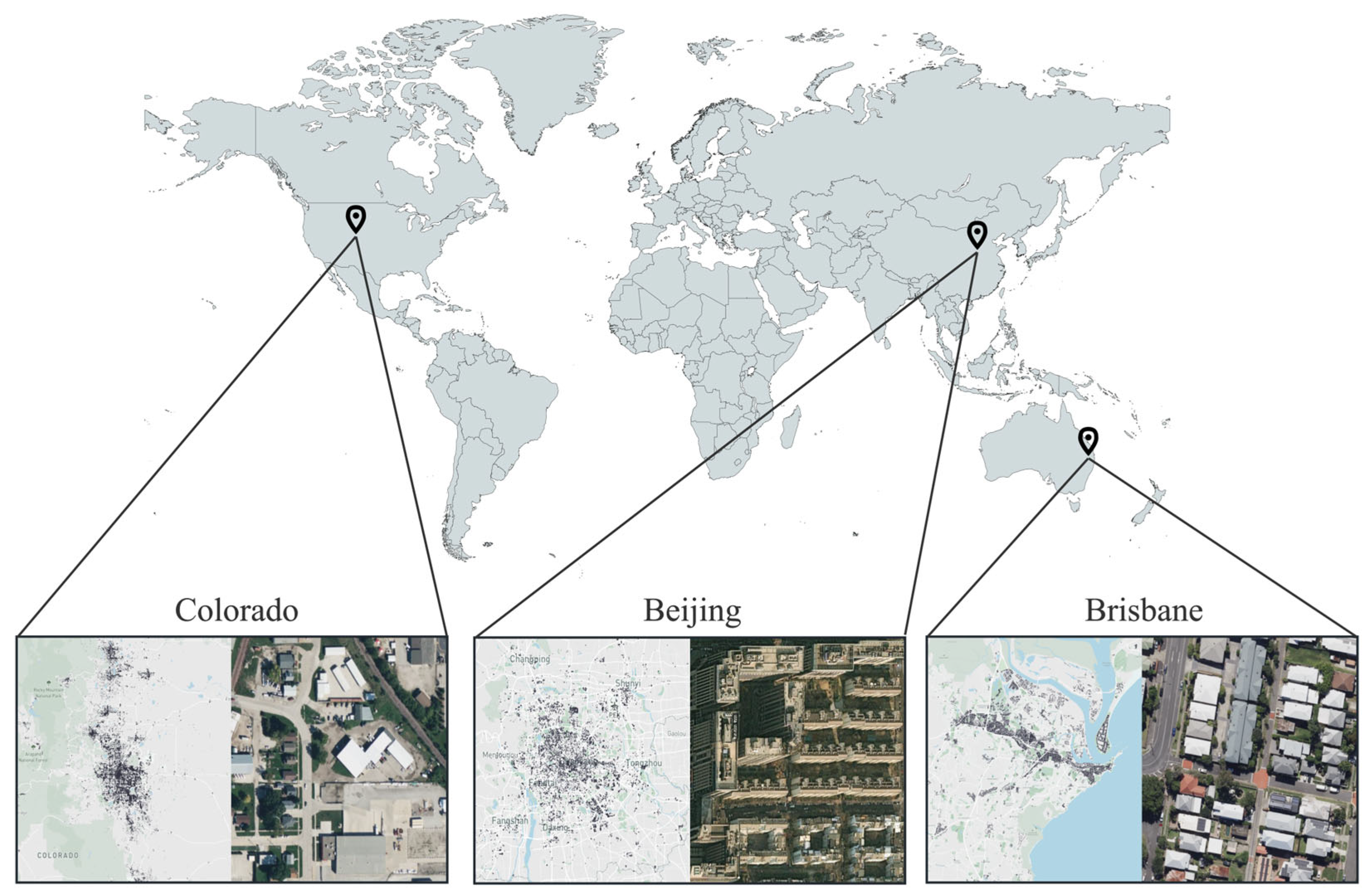
2.1.3. Public Test Area Dataset
2.2. Methods
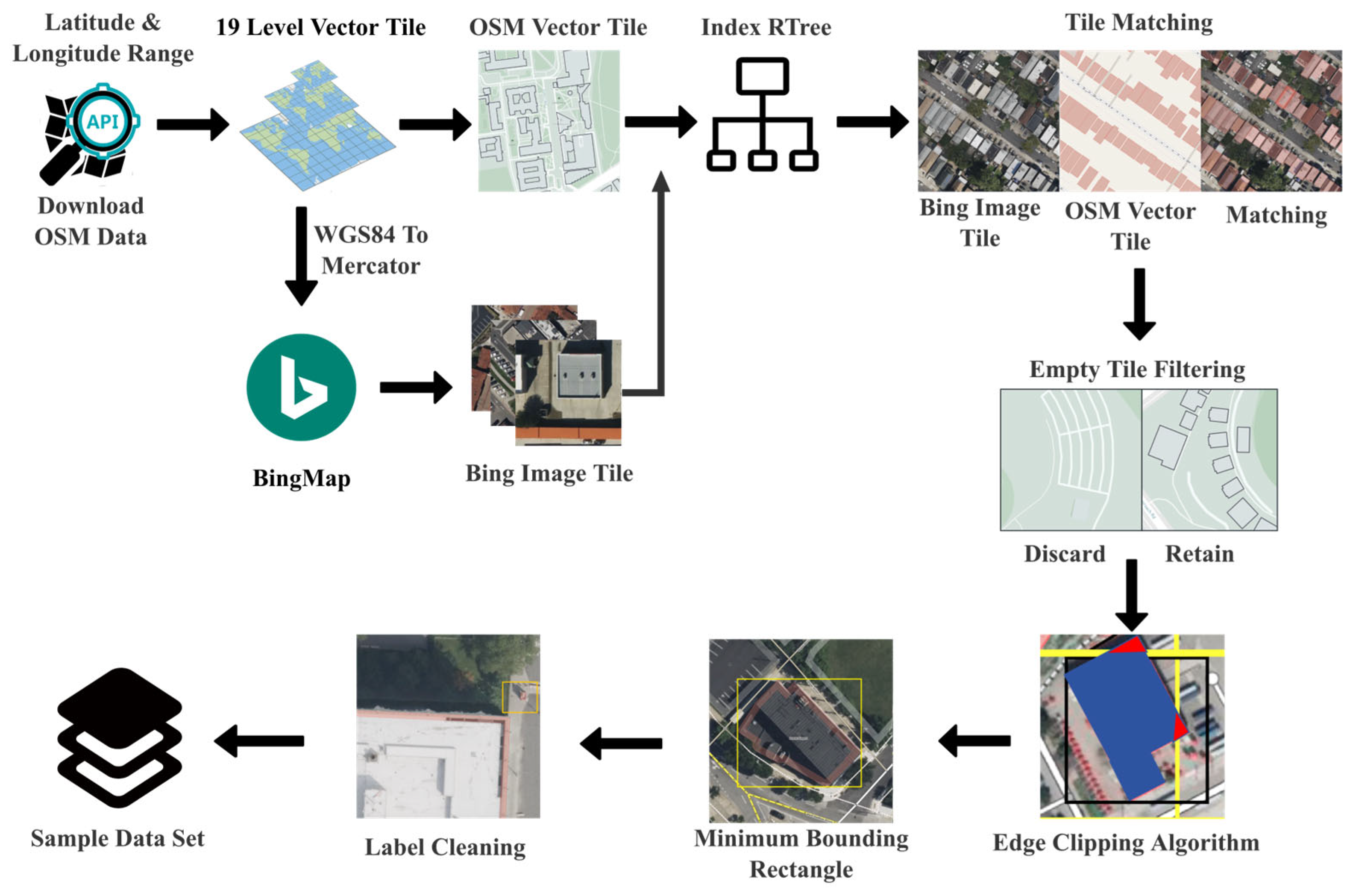
2.2.1. OSM Vector Data Definition
2.2.2. Parsing Algorithm and Implementation Principles
2.2.3. Projection Transformation
- 1.
- Web Mercator Projection Transformation
- 2.
- Tile Coordinate Calculation
- 3.
- Bing Map Image Tile Index Generation and Download
2.2.4. Category Mapping and Geometric Processing
- 1.
- Category Mapping
- 2.
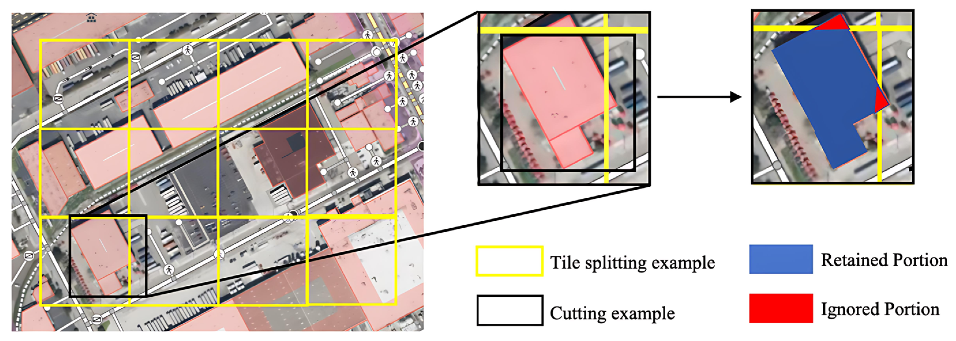
- Polygon Trimming and Bounding Box Calculation
- For each clipping edge;
- Sequentially process each edge of the original polygon and compute its intersections with the clipping boundary;
- Retain all vertices and intersection points that lie within the clipping region to form a new set of polygon vertices.
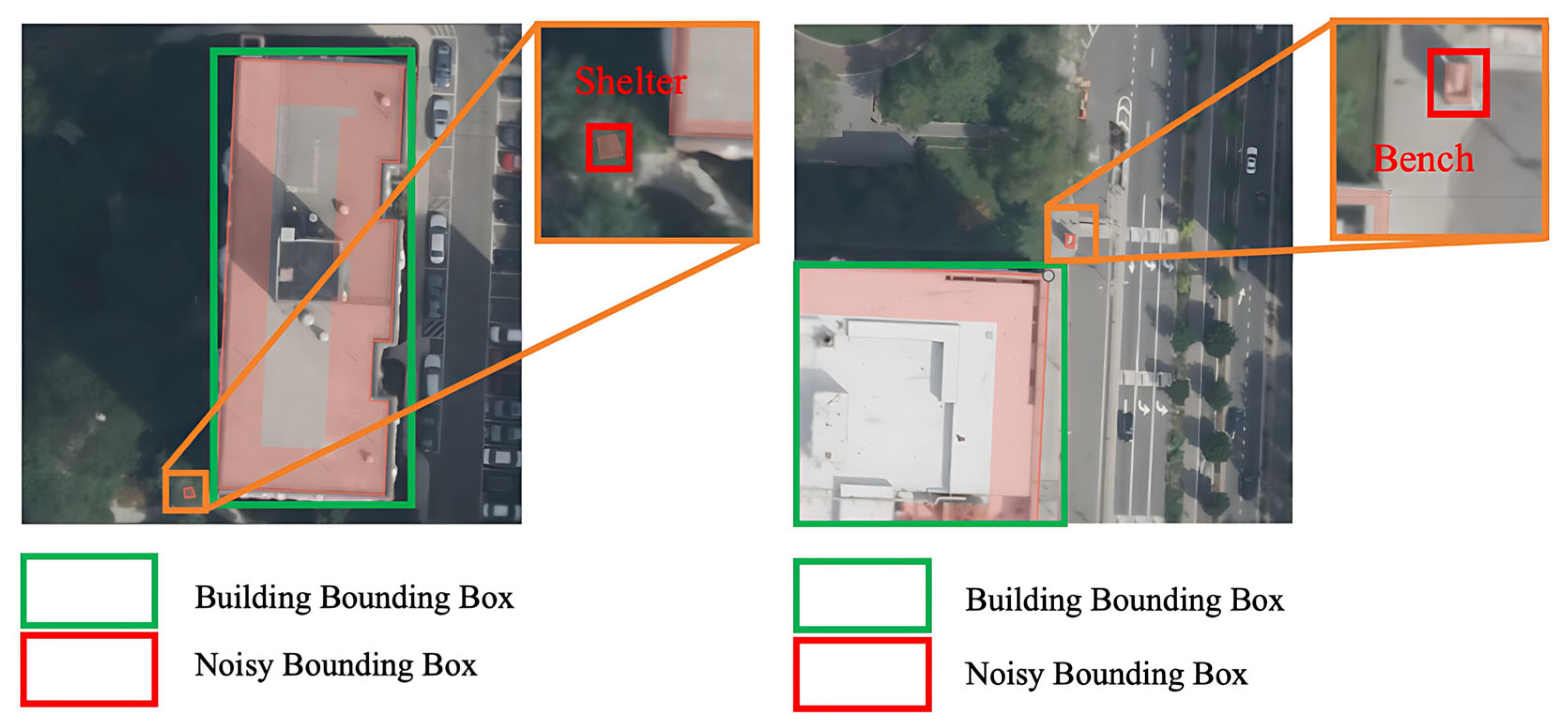
2.2.5. Label Cleaning
2.2.6. OSM Tag Quality Filtering Logic Based on Editing History
2.2.7. Sample Annotations Generation
2.2.8. Experimental Platform and Hyper-Parameter Settings
2.2.9. Evaluation of Experiments and Indicators
3. Results
3.1. Benchmark Performance Evaluation
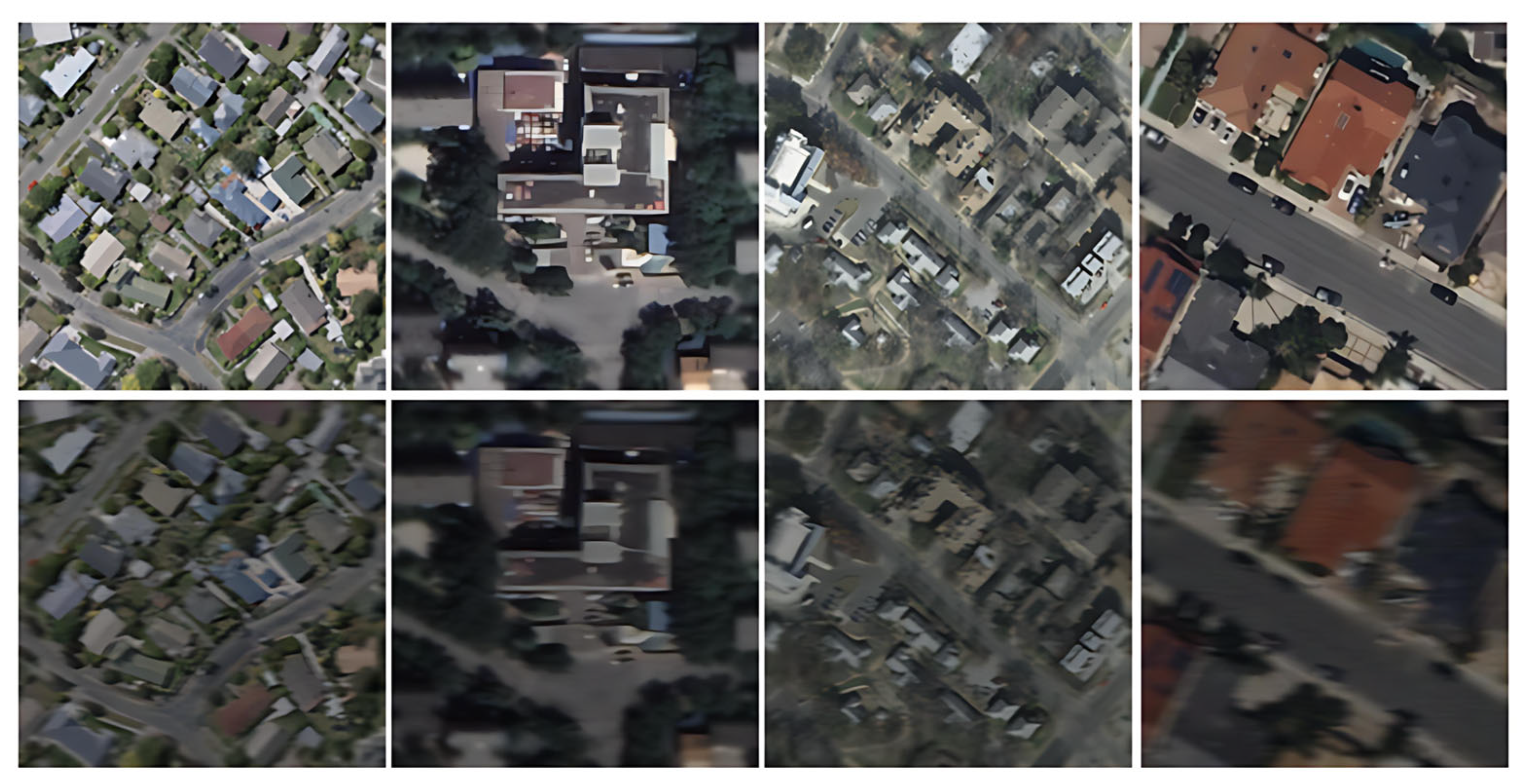
3.2. Input Perturbation Robustness Testing
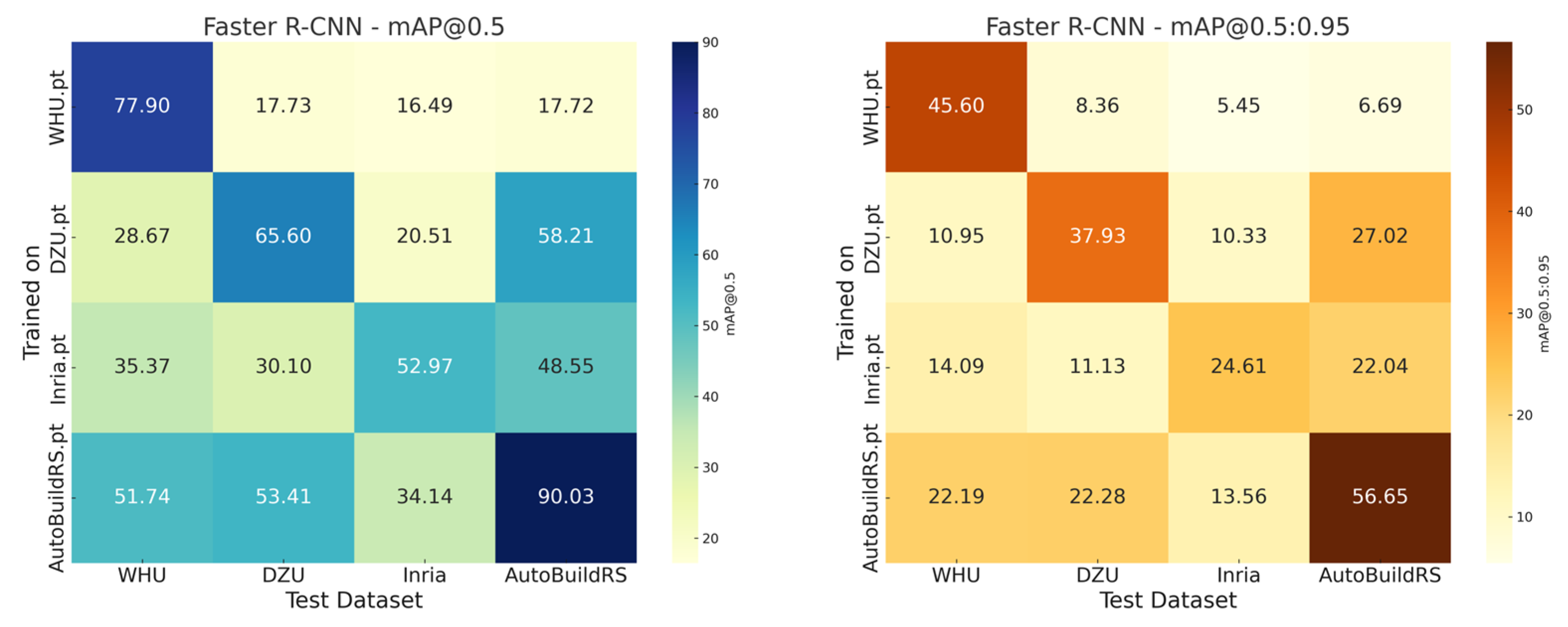
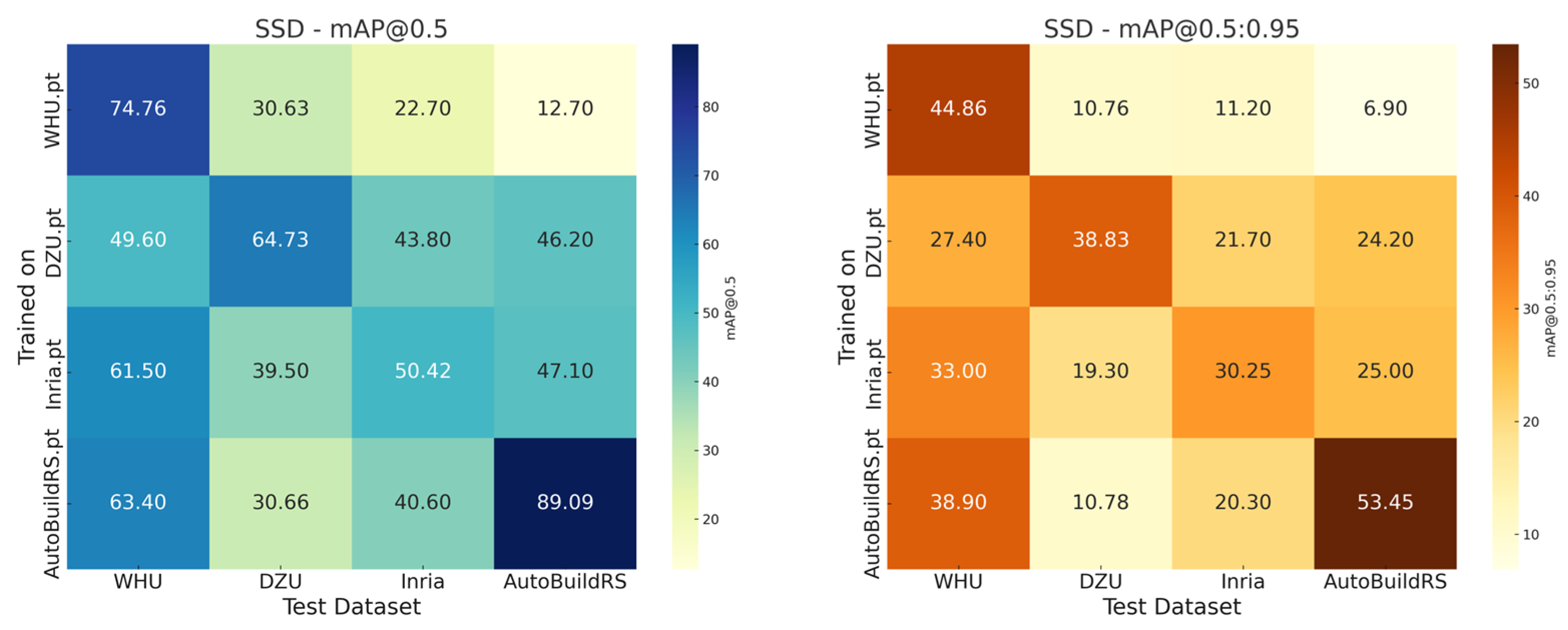
3.3. Cross-Dataset Generalization Analysis
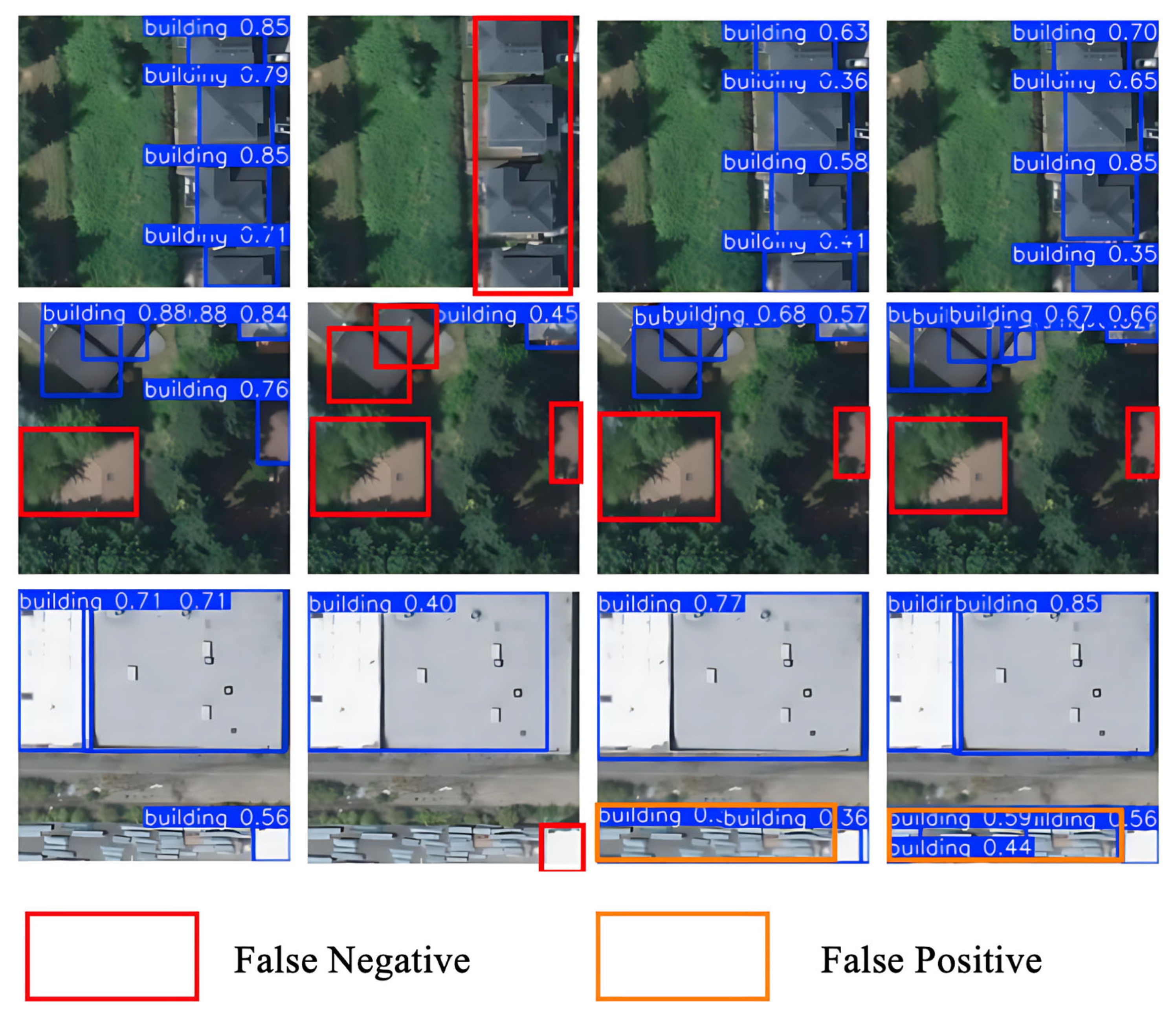
3.4. Comparative Experiments on Public Test Regions
4. Discussion
5. Conclusions
Author Contributions
Funding
Data Availability Statement
Conflicts of Interest
References
- Atwal, K.S.; Anderson, T.; Pfoser, D.; Züfle, A. Predicting building types using OpenStreetMap. Sci. Rep. 2022, 12, 19976. [Google Scholar] [CrossRef] [PubMed]
- Bagheri, H.; Schmitt, M.; Zhu, X. Fusion of multi-sensor-derived heights and OSM-derived building footprints for urban 3D reconstruction. ISPRS Int. J. Geo-Inf. 2019, 8, 193. [Google Scholar] [CrossRef]
- Zhang, W.; Tang, P.; Zhao, L. Remote sensing image scene classification using CNN-CapsNet. Remote Sens. 2019, 11, 494. [Google Scholar] [CrossRef]
- Sun, X.; Liu, L.; Li, C.; Yin, J.; Zhao, J.; Si, W. Classification for remote sensing data with improved CNN-SVM method. IEEE Access 2019, 7, 164507–164516. [Google Scholar] [CrossRef]
- Li, D.; Neira-Molina, H.; Huang, M.; Zhang, Y.; Junfeng, Z.; Bhatti, U.A.; Asif, M.; Sarhan, N.; Awwad, E.M. CSTFNet: A CNN and dual Swin-transformer fusion network for remote sensing hyperspectral data fusion and classification of coastal areas. IEEE J. Sel. Top. Appl. Earth Obs. Remote Sens. 2025, 18, 5853–5865. [Google Scholar] [CrossRef]
- Liu, L.; Wang, Y.; Peng, J.; Zhang, L. GLR-CNN: CNN-based framework with global latent relationship embedding for high-resolution remote sensing image scene classification. IEEE Trans. Geosci. Remote Sens. 2024, 62, 5633913. [Google Scholar] [CrossRef]
- Zaid, M.M.A.; Mohammed, A.A.; Sumari, P. Remote sensing image classification using convolutional neural network (CNN) and transfer learning techniques. arXiv 2025, arXiv:2503.02510. [Google Scholar]
- Feng, H.; Wang, Y.; Li, Z.; Zhang, N.; Zhang, Y.; Gao, Y. Information leakage in deep learning-based hyperspectral image classification: A survey. Remote Sens. 2023, 15, 3793. [Google Scholar] [CrossRef]
- Cheng, L.; Li, J.; Duan, P.; Wang, M. A small attentional YOLO model for landslide detection from satellite remote sensing images. Landslides 2021, 18, 2751–2765. [Google Scholar] [CrossRef]
- He, X.; Liang, K.; Zhang, W.; Li, F.; Jiang, Z.; Zuo, Z.; Tan, X. DETR-ORD: An Improved DETR Detector for Oriented Remote Sensing Object Detection with Feature Reconstruction and Dynamic Query. Remote Sens. 2024, 16, 3516. [Google Scholar] [CrossRef]
- Lu, X.; Ji, J.; Xing, Z.; Miao, Q. Attention and feature fusion SSD for remote sensing object detection. IEEE Trans. Instrum. Meas. 2021, 70, 5501309. [Google Scholar] [CrossRef]
- Wang, Q.; Zhang, X.; Chen, G.; Dai, F.; Gong, Y.; Zhu, K. Change detection based on Faster R-CNN for high-resolution remote sensing images. Remote Sens. Lett. 2018, 9, 923–932. [Google Scholar] [CrossRef]
- Wu, T.; Dong, Y. YOLO-SE: Improved YOLOv8 for remote sensing object detection and recognition. Appl. Sci. 2023, 13, 12977. [Google Scholar] [CrossRef]
- Yin, R.; Zhao, W.; Fan, X.; Yin, Y. AF-SSD: An accurate and fast single shot detector for high spatial remote sensing imagery. Sensors 2020, 20, 6530. [Google Scholar] [CrossRef] [PubMed]
- Ding, W.; Zhang, L. Building detection in remote sensing image based on improved YOLOv5. In Proceedings of the 2021 17th International Conference on Computational Intelligence and Security (CIS), Chengdu, China, 19–22 November 2021; pp. 133–136. [Google Scholar]
- Lin, J.; Zhao, Y.; Wang, S.; Tang, Y. YOLO-DA: An efficient YOLO-based detector for remote sensing object detection. IEEE Geosci. Remote Sens. Lett. 2023, 20, 6008705. [Google Scholar] [CrossRef]
- Sun, X.; Wang, P.; Yan, Z.; Xu, F.; Wang, R.; Diao, W.; Chen, J.; Li, J.; Feng, Y.; Xu, T. FAIR1M: A benchmark dataset for fine-grained object recognition in high-resolution remote sensing imagery. ISPRS J. Photogramm. Remote Sens. 2022, 184, 116–130. [Google Scholar] [CrossRef]
- Van Etten, A.; Lindenbaum, D.; Bacastow, T.M. Spacenet: A remote sensing dataset and challenge series. arXiv 2018, arXiv:1807.01232. [Google Scholar]
- Zhao, M.; Zhang, C.; Gu, Z.; Cao, Z.; Cai, C.; Wu, Z.; He, L. Automatic generation of high-quality building samples using OpenStreetMap and deep learning. Int. J. Appl. Earth Obs. Geoinf. 2025, 139, 104564. [Google Scholar] [CrossRef]
- Vargas-Munoz, J.E.; Srivastava, S.; Tuia, D.; Falcao, A.X. OpenStreetMap: Challenges and opportunities in machine learning and remote sensing. IEEE Geosci. Remote Sens. Mag. 2020, 9, 184–199. [Google Scholar] [CrossRef]
- Chen, K.; Fu, K.; Gao, X.; Yan, M.; Sun, X.; Zhang, H. Building extraction from remote sensing images with deep learning in a supervised manner. In Proceedings of the 2017 IEEE International Geoscience and Remote Sensing Symposium (IGARSS), Fort Worth, TX, USA, 23–28 July 2017; pp. 1672–1675. [Google Scholar]
- Huang, F.; Yu, Y.; Feng, T. Automatic building change image quality assessment in high resolution remote sensing based on deep learning. J. Vis. Commun. Image Represent. 2019, 63, 102585. [Google Scholar] [CrossRef]
- Hui, J.; Du, M.; Ye, X.; Qin, Q.; Sui, J. Effective building extraction from high-resolution remote sensing images with multitask driven deep neural network. IEEE Geosci. Remote Sens. Lett. 2018, 16, 786–790. [Google Scholar] [CrossRef]
- Luo, L.; Li, P.; Yan, X. Deep learning-based building extraction from remote sensing images: A comprehensive review. Energies 2021, 14, 7982. [Google Scholar] [CrossRef]
- Schuegraf, P.; Zorzi, S.; Fraundorfer, F.; Bittner, K. Deep learning for the automatic division of building constructions into sections on remote sensing images. IEEE J. Sel. Top. Appl. Earth Obs. Remote Sens. 2023, 16, 7186–7200. [Google Scholar] [CrossRef]
- Zeng, Y.; Guo, Y.; Li, J. Recognition and extraction of high-resolution satellite remote sensing image buildings based on deep learning. Neural Comput. Appl. 2022, 34, 2691–2706. [Google Scholar] [CrossRef]
- Fang, F.; Wu, K.; Liu, Y.; Li, S.; Wan, B.; Chen, Y.; Zheng, D. A Coarse-to-Fine Contour Optimization Network for Extracting Building Instances from High-Resolution Remote Sensing Imagery. Remote Sens. 2021, 13, 3814. [Google Scholar] [CrossRef]
- Fan, H.; Zipf, A.; Fu, Q. Estimation of building types on OpenStreetMap based on urban morphology analysis. In Connecting a Digital Europe Through Location and Place; Springer: Berlin/Heidelberg, Germany, 2014; pp. 19–35. [Google Scholar]
- Battersby, S. Web Mercator: Past, present, and future. Int. J. Cartogr. 2025, 11, 271–276. [Google Scholar] [CrossRef]
- Wada, T. On some information geometric structures concerning Mercator projections. Phys. A Stat. Mech. Its Appl. 2019, 531, 121591. [Google Scholar] [CrossRef]
- Ye, W.; Zhang, F.; He, X.; Bai, Y.; Liu, R.; Du, Z. A tile-based framework with a spatial-aware feature for easy access and efficient analysis of marine remote sensing data. Remote Sens. 2020, 12, 1932. [Google Scholar] [CrossRef]
- Ozge Unel, F.; Ozkalayci, B.O.; Cigla, C. The power of tiling for small object detection. In Proceedings of the IEEE/CVF Conference on Computer Vision and Pattern Recognition Workshops, Long Beach, CA, USA, 16–17 June 2019; pp. 0–0. [Google Scholar]
- Tulabandhula, T.; Nguyen, D. Dynamic Tiling: A Model-Agnostic, Adaptive, Scalable, and Inference-Data-Centric Approach for Efficient and Accurate Small Object Detection. arXiv 2023, arXiv:2309.11069. [Google Scholar]
- Varga, L.A.; Zell, A. Tackling the background bias in sparse object detection via cropped windows. In Proceedings of the IEEE/CVF International Conference on Computer Vision, Montreal, BC, Canada, 11–17 October 2021; pp. 2768–2777. [Google Scholar]
- Gao, J.; Chen, Y.; Wei, Y.; Li, J. Detection of specific building in remote sensing images using a novel YOLO-S-CIOU model. Case: Gas station identification. Sensors 2021, 21, 1375. [Google Scholar] [CrossRef] [PubMed]
- Zhang, H.; Ma, Z.; Li, X. Rs-detr: An improved remote sensing object detection model based on rt-detr. Appl. Sci. 2024, 14, 10331. [Google Scholar] [CrossRef]
- Chen, Y.; Huang, T.-Z.; Zhao, X.-L.; Deng, L.-J.; Huang, J. Stripe noise removal of remote sensing images by total variation regularization and group sparsity constraint. Remote Sens. 2017, 9, 559. [Google Scholar] [CrossRef]
- Cheng, G.; Huang, Y.; Li, X.; Lyu, S.; Xu, Z.; Zhao, H.; Zhao, Q.; Xiang, S. Change detection methods for remote sensing in the last decade: A comprehensive review. Remote Sens. 2024, 16, 2355. [Google Scholar] [CrossRef]
- Liu, J.; Wang, X.; Chen, M.; Liu, S.; Shao, Z.; Zhou, X.; Liu, P. Illumination and contrast balancing for remote sensing images. Remote Sens. 2014, 6, 1102–1123. [Google Scholar] [CrossRef]
- Ma, X.; Wang, Q.; Tong, X. Nighttime light remote sensing image haze removal based on a deep learning model. Remote Sens. Environ. 2025, 318, 114575. [Google Scholar] [CrossRef]
- Tsagkatakis, G.; Aidini, A.; Fotiadou, K.; Giannopoulos, M.; Pentari, A.; Tsakalides, P. Survey of deep-learning approaches for remote sensing observation enhancement. Sensors 2019, 19, 3929. [Google Scholar] [CrossRef] [PubMed]
- Gominski, D.; Gouet-Brunet, V.; Chen, L. Cross-dataset learning for generalizable land use scene classification. In Proceedings of the IEEE/CVF Conference on Computer Vision and Pattern Recognition, New Orleans, LA, USA, 18–24 June 2022; pp. 1382–1391. [Google Scholar]
- Rolf, E. Evaluation challenges for geospatial ML. arXiv 2023, arXiv:2303.18087. [Google Scholar]
- Zhang, X.; Huang, H.; Zhang, D.; Zhuang, S.; Han, S.; Lai, P.; Liu, H. Cross-Dataset Generalization in Deep Learning. arXiv 2024, arXiv:2410.11207. [Google Scholar]
- Bai, T.; Pang, Y.; Wang, J.; Han, K.; Luo, J.; Wang, H.; Lin, J.; Wu, J.; Zhang, H. An optimized faster R-CNN method based on DRNet and RoI align for building detection in remote sensing images. Remote Sens. 2020, 12, 762. [Google Scholar] [CrossRef]
- Liu, Y.; Zhang, Z.; Zhong, R.; Chen, D.; Ke, Y.; Peethambaran, J.; Chen, C.; Sun, L. Multilevel building detection framework in remote sensing images based on convolutional neural networks. IEEE J. Sel. Top. Appl. Earth Obs. Remote Sens. 2018, 11, 3688–3700. [Google Scholar] [CrossRef]
- Zhang, L.; Wu, J.; Fan, Y.; Gao, H.; Shao, Y. An efficient building extraction method from high spatial resolution remote sensing images based on improved mask R-CNN. Sensors 2020, 20, 1465. [Google Scholar] [CrossRef] [PubMed]
- Jung, S.; Song, A.; Lee, K.; Lee, W.H. Advanced Building Detection with Faster R-CNN Using Elliptical Bounding Boxes for Displacement Handling. Remote Sens. 2025, 17, 1247. [Google Scholar] [CrossRef]


| Dataset Attributes | WHU | INRIA | DZU | AutoBuildRS |
|---|---|---|---|---|
| Sample size | 8188 | 8820 | 7260 | 36,647 |
| Number of buildings | 196,016 | 177,809 | 47,081 | 154,703 |
| Spatial resolution (M) | 0.3 | 0.3 | 0.3 | 0.3 |
| Image size | 512 × 512 | 640 × 640 | 500 × 500 | 256 × 256 |
| Data Source | Aerial | Aerial | Satellite | Satellite |
| Release Date | 2018 | 2017 | 2023 | 2025 |
| ACR (α, β) | ACR Applied | mAP@0.5 (%) | Precision (%) | Recall (%) |
|---|---|---|---|---|
| α = 0, β = 0 | NO | 80.3 | 83.9 | 87.1 |
| α = 0.05, β = 0.7 | Yes | 85.3 | 87.9 | 88.4 |
| α = 0.10, β = 0.8 | Yes | 87.2 | 89.5 | 91.2 |
| α = 0.15, β = 0.9 | Yes | 83.4 | 89.2 | 78.4 |
| Dataset | Sample Size | Boxes Generated | Time (min) | Avg RAM | CPU Threads | GPU Used | Boxes/Sec |
|---|---|---|---|---|---|---|---|
| Washington, DC | 5490 | 34,931 | ~45 | ~8 G | 16 | No | 12 |
| New Zealand | 2391 | 43,917 | ~15 | ~7 G | 16 | No | 48 |
| Sydney | 2011 | 14,590 | ~15 | ~7 G | 16 | No | 16 |
| New York | 14,950 | 38,960 | ~100 | ~10 G | 16 | No | 6 |
| Los Angeles | 11,805 | 22,305 | ~85 | ~10 G | 16 | No | 4 |
| Name | Configuration |
|---|---|
| Operating System | Ubuntu 18.04.6 LTS |
| CPU | AMD Ryzen Threadripper 3970X, 32-Core × 64 threads |
| GPU | NVIDIA GeForce RTX 3090 × 3 |
| GPU Memory | 72 G |
| RAM | 125.7 G |
| CUDA | 11.5 |
| Pytorch | 1.12.1 |
| AutoBuildRS | mAP@0.5 | mAP@0.5:0.95 | Precision | Recall | F1-Score | FPS | Parameters (M) | GFLOPS | Weights (MB) |
|---|---|---|---|---|---|---|---|---|---|
| SSD300 | 89.09 | 53.45 | 86.12 | 86.55 | 86.33 | 45.19 | 23.75 | 30.43 | 95 |
| Faster-RCNN | 90.03 | 56.65 | 67.45 | 93.22 | 78 | 21.33 | 28.28 | 940.92 | 113.4 |
| DETR | 91.54 | 77.83 | N/A * | N/A * | N/A * | N/A * | 41.28 | 58.1 | 497 |
| YOLOv11s | 93.2 | 73.7 | 89.4 | 90.6 | 89.99 | 128.21 | 9.41 | 21.5 | 19.2 |
| WHU | mAP@0.5 | mAP@0.5:0.95 | Precision | Recall | F1-Score | FPS | Parameters (M) | GFLOPS | Weights (MB) |
|---|---|---|---|---|---|---|---|---|---|
| SSD300 | 74.76 | 44.86 | 93.2 | 57.76 | 71.32 | 45.27 | 23.75 | 30.43 | 95 |
| Faster-RCNN | 77.9 | 45.6 | 75.37 | 78.38 | 76.85 | 20.07 | 28.28 | 940.92 | 113.4 |
| DETR | 90.51 | 68.65 | N/A * | N/A * | N/A * | N/A * | 41.28 | 58.1 | 497 |
| YOLOv11s | 93.8 | 76.6 | 92.7 | 87.3 | 89.92 | 136.99 | 9.41 | 21.5 | 19.2 |
| DZU | mAP@0.5 | mAP@0.5:0.95 | Precision | Recall | F1-Score | FPS | Parameters (M) | GFLOPS | Weights (MB) |
|---|---|---|---|---|---|---|---|---|---|
| SSD300 | 64.73 | 38.83 | 74.94 | 56.15 | 64.2 | 43.03 | 23.75 | 30.43 | 95 |
| Faster-RCNN | 65.83 | 43.23 | 64.96 | 67.13 | 66.03 | 20.23 | 28.28 | 940.92 | 113.4 |
| DETR | 71.12 | 47.82 | N/A * | N/A * | N/A * | N/A * | 41.28 | 58.1 | 497 |
| YOLOv11s | 75.6 | 55.2 | 73.2 | 68.4 | 70.72 | 131.58 | 9.41 | 21.5 | 19.2 |
| INRIA | mAP@0.5 | mAP@0.5:0.95 | Precision | Recall | F1-Score | FPS | Parameters (M) | GFLOPS | Weights (MB) |
|---|---|---|---|---|---|---|---|---|---|
| SSD300 | 50.42 | 30.25 | 84.35 | 35.8 | 50.27 | 42.93 | 23.75 | 30.43 | 95 |
| Faster-RCNN | 52.91 | 24.67 | 56.87 | 58.47 | 58 | 20.15 | 28.28 | 940.92 | 113.4 |
| DETR | 64.14 | 34.10 | N/A * | N/A * | N/A * | N/A * | 41.28 | 58.1 | 497 |
| YOLOv11s | 83.3 | 59.5 | 88 | 76.8 | 82.02 | 135.14 | 9.41 | 21.5 | 19.2 |
| Disturbance Condition | Dataset | Clean mAP@0.5 | Perturbed mAP@0.5 | RAR | AAD | SRS |
|---|---|---|---|---|---|---|
| 25/0.7/13 | WHU | 93.8 | 90.6 | 3.41% | 3.2 | 0.97 |
| DZU | 75.6 | 71.5 | 5.42% | 4.1 | 0.95 | |
| INRIA | 83.3 | 74.3 | 10.81% | 9 | 0.89 | |
| AutoBuildRS | 93.2 | 91.9 | 1.39% | 1.3 | 0.99 | |
| 35/0.6/17 | WHU | 93.8 | 89.4 | 4.69% | 4.4 | 0.95 |
| DZU | 75.6 | 69.9 | 7.54% | 5.7 | 0.92 | |
| INRIA | 83.3 | 70.9 | 14.89 | 12.4 | 0.85 | |
| AutoBuildRS | 93.2 | 91 | 2.36% | 2.2 | 0.98 | |
| 45/0.5/21 | WHU | 93.8 | 88.8 | 5.33% | 5 | 0.95 |
| DZU | 75.6 | 68.9 | 8.86% | 6.7 | 0.91 | |
| INRIA | 83.3 | 70.9 | 14.89 | 12.4 | 0.85 | |
| AutoBuildRS | 93.2 | 90.4 | 3% | 2.8 | 0.97 |
| Models | Weights | mAP@0.5 | mAP@0.5:0.95 | Precision | Recall | F1-Score | FPS |
|---|---|---|---|---|---|---|---|
| YOLOv11s | WHU.pt | 17.9 | 11.2 | 35.7 | 0.08 | 0.16 | 136.9 |
| DZU.pt | 58 | 29.1 | 58.2 | 60 | 59.07 | 129.9 | |
| INRIA.pt | 61.3 | 32.1 | 63.2 | 59.2 | 61.13 | 125 | |
| AutoBuildRS.pt | 85.7 | 50.7 | 83.3 | 82.7 | 83 | 131.58 | |
| Faster R-CNN | WHU.pt | 25.22 | 10.55 | 16.50 | 14.72 | 15.56 | 23.48 |
| DZU.pt | 69.93 | 33.38 | 41.40 | 96.21 | 57.88 | 22.69 | |
| INRIA.pt | 65.60 | 30.50 | 48.14 | 87.21 | 62.03 | 23.34 | |
| AutoBuildRS.pt | 83.88 | 44.16 | 66.82 | 89.30 | 76.44 | 23.60 | |
| DETR | WHU.pt | 26.08 | 12.15 | N/A * | N/A * | N/A * | N/A * |
| DZU.pt | 55.19 | 27.72 | N/A * | N/A * | N/A * | N/A * | |
| INRIA.pt | 59.58 | 30.27 | N/A * | N/A * | N/A * | N/A * | |
| AutoBuildRS.pt | 84.74 | 49.30 | N/A * | N/A * | N/A * | N/A * | |
| SSD | WHU.pt | 14.08 | 11.20 | 62.17 | 16.77 | 26.47 | 30.91 |
| DZU.pt | 58.55 | 33 | 71.75 | 65.77 | 68.63 | 23.33 | |
| INRIA.pt | 55.71 | 34.90 | 79.88 | 60.85 | 69.07 | 23.60 | |
| AutoBuildRS.pt | 72.45 | 45.40 | 86.81 | 76.72 | 81.12 | 23.81 |
Disclaimer/Publisher’s Note: The statements, opinions and data contained in all publications are solely those of the individual author(s) and contributor(s) and not of MDPI and/or the editor(s). MDPI and/or the editor(s) disclaim responsibility for any injury to people or property resulting from any ideas, methods, instructions or products referred to in the content. |
© 2025 by the authors. Licensee MDPI, Basel, Switzerland. This article is an open access article distributed under the terms and conditions of the Creative Commons Attribution (CC BY) license (https://creativecommons.org/licenses/by/4.0/).
Share and Cite
Gu, J.; Ji, C.; Chen, H.; Zheng, X.; Jiao, L.; Cheng, L. A Method for Auto Generating a Remote Sensing Building Detection Sample Dataset Based on OpenStreetMap and Bing Maps. Remote Sens. 2025, 17, 2534. https://doi.org/10.3390/rs17142534
Gu J, Ji C, Chen H, Zheng X, Jiao L, Cheng L. A Method for Auto Generating a Remote Sensing Building Detection Sample Dataset Based on OpenStreetMap and Bing Maps. Remote Sensing. 2025; 17(14):2534. https://doi.org/10.3390/rs17142534
Chicago/Turabian StyleGu, Jiawei, Chen Ji, Houlin Chen, Xiangtian Zheng, Liangbao Jiao, and Liang Cheng. 2025. "A Method for Auto Generating a Remote Sensing Building Detection Sample Dataset Based on OpenStreetMap and Bing Maps" Remote Sensing 17, no. 14: 2534. https://doi.org/10.3390/rs17142534
APA StyleGu, J., Ji, C., Chen, H., Zheng, X., Jiao, L., & Cheng, L. (2025). A Method for Auto Generating a Remote Sensing Building Detection Sample Dataset Based on OpenStreetMap and Bing Maps. Remote Sensing, 17(14), 2534. https://doi.org/10.3390/rs17142534