Angular Super-Resolution of Forward-Looking Scanning Radar via Grid-Updating Split SPICE-TV

Abstract

The sparse iterative covariance-based estimation (SPICE) method has recently gained significant attraction in the field of scanning radar super-resolution imaging because of its angular resolution enhancement capability. However, it is unable to preserve the target profile, and the estimator is constrained by high computational complexity and memory consumption. In this paper, a grid-updating split SPICE-TV algorithm is presented. The method allows for the efficient updating of reconstruction results with both contour and resolution, and a recursive grid-updating implementation framework of the split SPICE-TV has the capability to reduce the computational complexity. First, the scanning radar angular super-resolution problem is transformed into a constrained optimization problem by simultaneously employing sparse covariance fitting criteria and TV regularization constraints. Then, the split Bregman method is employed to derive an efficient closed-form solution to the problem. Ultimately, the matrix inversion problem is transformed into an online iterative equation to reduce the computational complexity and memory consumption. The superiority of the proposed method is verified by simulation and experimental data.

1. Introduction

The scanning radar is widely utilized in various fields, including aircraft autonomous landing, material airdrop, and ground attack [1,2,3]. However, its angular resolution is limited to the size of the radar aperture in the forward-looking directions. Especially for airborne platforms, it is challenging to provide the necessary space resources [4,5], leading to low angular resolution. The conventional synthetic aperture radar (SAR) methodology encounters challenges in forward-looking imaging as a result of the concurrence of the equal-distance and equal-Doppler lines within the forward-looking zone [6,7,8]. Doppler beam sharpening (DBS) encounters difficulties in the resolution of forward-looking imaging due to the symmetry issues and the reduction in the Doppler centroid gradient [9,10]. Based on the scanning mode of radar beam, angular super-resolution methods have been studied to improve the angular resolution depending on the convolution signal model between the antenna pattern and target scatterings.

The super-resolution imaging methods are proposed from different perspectives, such as spectral estimation-based methods [11,12,13], Bayesian methods [4,14,15] and regularization methods [16,17,18,19,20]. In [11], a fast conjugate gradient iterative adaptive algorithm-based spectral estimation approach was developed for forward-looking super-resolution imaging. This approach can accurately model velocity migration across different directions, decouple range and azimuth-elevation dependencies, and enhance target resolution efficiency. However, it only constructs the echo covariance matrix based on a specific range bin, which is difficult applied in low signal-to-noise ratios (SNRs) and limited snapshots conditions. Alternatively, an efficient Bayesian forward-looking super-resolution imaging algorithm [4] was proposed by reformulating the imaging task as a convex optimization problem. However, the method suffers from high computational complexity and prior distribution sensitivity. To avoid the reliance on idealized models of spectral estimation methods and the high computational costs of Bayesian approaches, the regularization methods was proposed based on sparse $L_1$ norm constraints [20]. However, the penalty parameters of the regularization methods should be manually adjusted according to the actual environment.

To leverage sparsity, reference [21] introduces the Sparse Iterative Covariance Estimation (SPICE). Experimental results demonstrate that this method offers a higher angular resolution compared to the Iterative Adaptive Approach (IAA). However, when the target exhibits distinct edge characteristics, the SPICE method fails to reconstruct the detailed contours of the target. To reconstruct contour information of the target, a total variation (TV) regularization method [22] has been introduced for scanning radar super-resolution imaging. This method uses the TV norm as a penalty term to preserve edge details and achieve high-quality imaging. It preserves the edge contours of the target, but it is no significant enhancement in angular resolution.

To address the aforementioned challenge of simultaneously enhancing angular resolution and preserving target contours, researchers have developed multimodal fusion techniques [23,24,25]. For instance, reference [23] achieved significant improvement in emotion recognition accuracy by integrating local convolutional features with global transformer attention through cross-modal transformers. Similarly, in the radar domain, such multimodal fusion approaches [26,27,28,29] have demonstrated potential for enhancing detection capabilities.

To enhance angular resolution and preserve target contours simultaneously, a super-resolution imaging method for scanning radar called SPICE-TV was proposed in [30]. However, this method employs MATLAB’s CVX toolbox to solve the joint optimization problem of SPICE-TV, and it does not offer a closed-form solution, which leading to significant computational costs. Furthermore, a split SPICE-TV method [31] is proposed by deriving a closed-form solution of the SPICE-TV method using the split Bregman method. Nevertheless, the method necessitates the inversion of a high-dimensional matrix on numerous occasions, and it is only capable of batch processing the entirety of the scanned data.

To reduce computational complexity and enable real-time processing, several online angular super-resolution methods have been put forth, primarily based on beam recursion approaches. In [32], an online Tikhonov method is proposed to achieve real-time super-resolution capability, but it delivers limited resolution improvement. The subsequent online q-SPICE method [33] can significantly enhance angular resolution, but the improvement comes at the expense of losing target contour reconstruction. The total variation method [34] can address this limitation by accurately recovering target contours, though its angular resolution performance remains constrained.

In order to address the aforementioned issues, this paper introduces a grid-updating split SPICE-TV super-resolution method. The method allows for the efficient updating of reconstruction results with both contour and resolution, and a recursive grid-updating implementation framework of the split SPICE-TV has the capability to reduce the computational complexity. First, the scanning radar angular super-resolution problem is transformed into a constrained optimization problem by simultaneously employing sparse covariance fitting criteria and TV regularization constraints. Then, the split Bregman method is employed to derive an efficient closed-form solution to the problem. Ultimately, the matrix inversion problem is transformed into an online iterative equation to reduce the computational complexity and memory consumption. The proposed method offers two advantages. On the one hand, the spatial complexity of the proposed method remains constant throughout the beam recursion process, and does not increase with time. On the other hand, the online grid-updating procedure can reduce the number of iterations, improving the processing efficiency and imaging quality without additional computational burden.

The arrangement of this paper is as follows. Section 2 introduces the echo model of the real aperture scanning radar. Section 3 presents the proposed method. Section 4 and Section 5 provide the simulation and measured data results. Finally, Section 6 concludes the paper.

2. Problem Analysis

This section details the modeling of scanning radar echoes and provides a comparative retrospective analysis between sparse iterative covariance fitting estimation and traditional TV methods.

2.1. Echo Model

The geometric motion model of the forward-looking scanning radar, as illustrated in Figure 1, involves an aircraft flying at a height H and moving with a velocity v along the Y-axis. The radar beam sweeps counterclockwise at an angular velocity w, with a pitch angle $\alpha$ at time $t=0$ when the aircraft is positioned at point A. At time t, assume there is a target P in space located at a distance $R_0$ from point A, with a horizontal azimuth of ${\phi }_0$ and a spatial azimuth of ${\theta }_0$. The geometric relationships yield the equation $cos{\theta }_0=cos{\phi }_{0}cos\alpha$.

At time t, as the aircraft transitions from point A to point B, the target P is characterized by a horizontal azimuth $\phi$ relative to the aircraft and a spatial azimuth $\theta$. The distance between the aircraft and the target P can be represented as

$$\begin{array}{c}\hfill R\left(t\right)=\sqrt{R_0^2+{\left(vt\right)}^2-2R_{0}vtcos{\theta }_0}\end{array}$$

(1)

Expanding $R\left(t\right)$ in a Taylor series around $t=0$ yields

$$\begin{array}{c}\hfill R\left(t\right)=R_0-vcos{\theta }_{0}t+{\displaystyle \frac{v^2{sin}^2{\theta }_0}{2R_0}}{t}^2\end{array}$$

(2)

Given that $v^2{t}^2$ (the product of velocity squared and time squared) is significantly smaller than the target distance, and $sin{\theta }_0\approx 0$ in the forward-looking region, the second-order Taylor expansion term becomes negligible [35]. Thus, the approximation for $R\left(t\right)$ simplifies to

$$\begin{array}{c}\hfill R\left(t\right)\approx R_0-vcos{\theta }_{0}t\end{array}$$

(3)

The forward-looking scanning radar emits wideband linear frequency modulation (FM) signals, resulting in

$$\begin{array}{c}\hfill S\left(\tau \right)=\mathrm{rect}\left({\displaystyle \frac{\tau }{T_r}}\right)exp\left(j2\pi f_0\tau +j\pi K_r{\tau }^2\right)\end{array}$$

(4)

where $\tau$ is the fast time variable in the range direction, $T_r$ is the pulse width of the linear FM signal, $f_0$ is the carrier frequency, $K_r$ is the frequency modulation slope, and $\mathrm{rect}\left(·\right)$ is the window function:

$$\begin{array}{c}\hfill \mathrm{rect}\left({\displaystyle \frac{\tau }{T_r}}\right)=\left\{\begin{array}{cc}1,\hfill & \mathrm{if}\tau <{\displaystyle \frac{T_r}{2}},\hfill \\ 0,\hfill & \mathrm{otherwise}.\hfill \end{array}\right.\end{array}$$

(5)

After down-conversion, the echo signal of target P can be expressed as

$$\begin{array}{c}\hfill S(\tau ,t)={\sigma }_{0}f\left(t\right)\mathrm{rect}\left({\displaystyle \frac{\tau -{\tau }_d}{T_r}}\right)exp\left(j\pi K_r{(\tau -{\tau }_d)}^2\right)exp\left(-j2\pi f_0{\tau }_d\right)\end{array}$$

(6)

where ${\sigma }_0$ is the target-scattering coefficient of P, $f\left(t\right)$ is the antenna pattern modulation function, t is the slow time variable in the azimuth direction, ${\tau }_d=2R\left(t\right)/c$ is the echo delay, and c is the speed of the electromagnetic wave.

By applying pulse compression to the echo signal, we obtain

$$\begin{array}{c}\hfill S_{rc}(\tau ,t)={\sigma }_{0}f\left(t\right)\sin \mathrm{c}\left[B(\tau -{\tau }_d)\right]exp\left(-j2\pi f_0{\tau }_d\right)\end{array}$$

(7)

where $\sin \mathrm{c}\left[·\right]$ is the range pulse compression response function, and B is the transmitted signal bandwidth.

After pulse compression, in scenarios involving low-speed platforms, the Doppler term $exp\left(-j2\pi f_0{\tau }_d\right)$ is disregarded. For all detectable targets, the azimuth echo signal is equivalent to the convolution between the antenna’s azimuth pattern function and the target-scattering characteristics, expressed as

$$\begin{array}{c}\hfill {\overline{S}}_{rc}\left(\tau ,t\right)=\int \int {\sigma }_{0}f\left(t\right)\sin \mathrm{c}\left[B\left(\tau -{\tau }_d\right)\right]\mathrm{d}\tau \mathrm{d}t\end{array}$$

(8)

Considering a random target’s range and azimuth angle in this space as R and $\theta$, respectively, we can derive

$$\begin{array}{c}\hfill \left\{\begin{array}{c}\tau ={\displaystyle \frac{2R}{c}}\hfill \\ t={\displaystyle \frac{\theta -{\theta }_0}{\omega }}\hfill \end{array}\right.\end{array}$$

(9)

Substituting Equation (9) into Equation (8) yields

$$\begin{array}{c}\hfill {\overline{S}}_{rc}\left(R,\theta \right)=\int \int {\sigma }_0\sin \mathrm{c}\left[{\displaystyle \frac{2B}{c}}\left(R-R_d\right)\right]f\left(\theta -{\theta }_0\right)\mathrm{d}R\mathrm{d}\theta \end{array}$$

(10)

Equation (10) can be reformulated in convolution form

$$\begin{array}{c}\hfill {\overline{S}}_{rc}\left(R,\theta \right)=\sigma \left(R,\theta \right)\ast h\left(R,\theta \right)\end{array}$$

(11)

where $h\left(R,\theta \right)$ is the antenna pattern function and $\sigma \left(R,\theta \right)$ is the effective scattering function. The discretization of (11) yields [36,37]

$$\begin{array}{c}\hfill \mathbf{y}=\mathbf{Hx}+\mathbf{e}\end{array}$$

(12)

where $\mathbf{y}\in {\mathbb{C}}^N$ represents the echo, N is the sampling number of the azimuthal echo, $\mathbf{x}\in {\mathbb{C}}^N$ is the scattering coefficient of the target, $\mathbf{e}\in {\mathbb{C}}^N$ is the additive noise, and $\mathbf{H}\in {\mathbb{C}}^{N\times N}$ is the pattern function of the antenna.

In this paper, the echo is neglected as the beam scans in and out of the scene, prompting the adoption of a truncated antenna pattern matrix, accurately expressed as

$$\begin{array}{c}\hfill \mathbf{H}={\left[\begin{array}{ccccc}{h}_{\left({\theta }_0\right)}& \cdots & h_{\left({\theta }_{-l}\right)}& & \\ ⋮& \ddots & & \ddots & \\ h_{\left({\theta }_l\right)}& & \ddots & & h_{\left({\theta }_{-l}\right)}\\ & \ddots & & \ddots & ⋮\\ & & h_{\left({\theta }_l\right)}& \cdots & h_{\left({\theta }_0\right)}\end{array}\right]}_{N\times N}\end{array}$$

(13)

where $\left[h_{\left({\theta }_{-l}\right)}\cdots h_{\left({\theta }_0\right)}\cdots h_{\left({\theta }_l\right)}\right]$ represents samples of the antenna pattern. The number of samples is determined by the pulse repetition frequency, beamwidth, and antenna scanning velocity.

2.2. Sparse Iterative Covariance Fitting Estimation

The deconvolution operation in the above model poses an ill-posed problem, typically addressed using regularization methods. To estimate sparse distributed targets in practical scenarios such as airports and seaports, the sparse covariance fitting criterion is defined as follows:

$$\begin{array}{c}\hfill f={∥{\mathbf{R}}^{-{\displaystyle \frac{1}{2}}}\left(\mathbf{y}{\mathbf{y}}^H-\mathbf{R}\right)∥}_F^2\end{array}$$

(14)

where

$$\begin{array}{c}\hfill \mathbf{R}=\mathbf{AB}{\mathbf{A}}^{*}\end{array}$$

(15)

$$\begin{array}{c}\hfill \mathbf{A}=\left[\mathbf{H}\mathbf{I}\right]\triangleq \left[{\mathbf{a}}_1{\mathbf{a}}_2\cdots {\mathbf{a}}_N\right]\end{array}$$

(16)

$$\begin{array}{c}\hfill \begin{array}{c}\mathbf{B}=diag\left(\left[{\left|x_1\right|}^2{\left|x_2\right|}^2\cdots {\left|x_K\right|}^2{\sigma }_1{\sigma }_2\cdots {\sigma }_N\right]\right)\hfill \\ \triangleq diag\left(\left[{\mathbf{b}}_1{\mathbf{b}}_2\cdots {\mathbf{b}}_{K+N}\right]\right)\hfill \end{array}\end{array}$$

(17)

where ${∥·∥}_F$ denotes the Frobenius norm, $\mathbf{I}$ is the $N\times N$ identity matrix, ${\mathbf{a}}_i$ represents the column vector of matrix $\mathbf{A}$, $diag\left(·\right)$ indicates a diagonal matrix, and ${\sigma }_n$ represents the noise variance. Referring to [38], minimizing Equation (14) leads to

$$\begin{array}{c}\hfill \underset{p_n>0}{min}{\mathbf{y}}^H{\mathbf{R}}^{-1}\mathbf{y}+{∥\mathbf{Wp}∥}_1\end{array}$$

(18)

where $w_j={\displaystyle \frac{∥{\mathbf{a}}_n∥}{{∥\mathbf{y}∥}^2}},j=1,2,\cdots ,N+K$, $\mathbf{W}=diag\left(\left[w_1{w}_2\cdots w_{K+N}\right]\right)$

Since the constraint term of SPICE involves a weighted $L_1$ norm, this method demonstrates significant advantages in enhancing target resolution; however, it fails to preserve the edge information of the targets. Consequently, it is not suitable for reconstructing targets with sharp outlines. While iterative reweighting and the MM method can be employed for batch processing, they tend to have high complexity. To mitigate this, online grid-updating can be performed using the loop minimization criterion [33], which helps reduce the overall complexity.

2.3. Traditional TV Method

Although the aforementioned method significantly enhances the resolution of point targets, it is ineffective in reconstructing the edge contours and scale information of extended targets. As an effective image processing technique, the total variation (TV) can preserve edge information and suppress noise by incorporating total variation regularization. This approach is more effective in reconstructing the edge contours and scale information of extended targets, thereby improving the overall quality and usability of the image. The total variation norm is conventionally expressed using a 2D gradient operator:

$$\begin{array}{c}\hfill {∥\mathbf{x}∥}_{TV}=\sum _{i,j}\left(\left|{\left({\nabla }_{\mathrm{azimuth}}\mathbf{x}\right)}_{ij}\right|+\left|{\left({\nabla }_{\mathrm{range}}\mathbf{x}\right)}_{ij}\right|\right)\end{array}$$

(19)

where ${\nabla }_{\mathrm{azimuth}}$ and ${\nabla }_{\mathrm{range}}$ represent the reciprocals in the azimuthal and range directions, respectively. To address the low azimuthal resolution issue in scanning radar, this paper employs the anisotropic total variation norm to obtain gradient information in the azimuthal direction of targets:

$$\begin{array}{c}\hfill {∥\mathbf{x}∥}_{TV}={∥\nabla \mathbf{x}∥}_1\end{array}$$

(20)

where ∇ denotes the azimuthal reciprocal, and for optimization expression, the subscript “azimuth” is omitted. The azimuthal reciprocal operator is defined as $\nabla \mathbf{x}=x_{i+1}-x_i,i=1,2,\cdots ,N-1$, and thus ∇ can be represented in matrix form as

$$\begin{array}{c}\hfill \nabla =\left[\begin{array}{ccccc}-1& 1& & & \\ & -1& 1& & \\ & & \ddots & \ddots & \\ & & & -1& 1\\ & & & & -1\end{array}\right]\end{array}$$

(21)

The total variation norm fundamentally constitutes a gradient-based operator. In radar-imaging applications, target boundaries exhibit substantial amplitude fluctuations, resulting in enhanced gradient magnitudes. Leveraging these properties by imposing the total variation norm as a regularization constraint enables accurate edge feature recovery. Consequently, the corresponding objective function takes the form

$$\begin{array}{c}\hfill J=\underset{\mathbf{x}}{min}{∥\mathbf{y}-\mathbf{Hx}∥}_2^2+\mu {∥\nabla \mathbf{x}∥}_1\end{array}$$

(22)

where $\underset{\mathbf{x}}{min}{∥\mathbf{y}-\mathbf{Hx}∥}_2$ serves as the data fidelity term, approximating the original target. $\mu {∥\nabla \mathbf{x}∥}_1$ is utilized to maintain edge constraints on the azimuthal angle’s edge details. $\mu$ denotes the regularization parameter for the TV term, balancing the level of resolution and edge constraint.

While Equation (22) can be addressed through batch processing using either the Bregman or MM methods, its computational complexity remains prohibitively high for online implementation. As demonstrated in [34], leveraging inter-pulse correlation allows the conversion of matrix inversion into iterative matrix multiplication operations. This approach enables sequential echo processing for real-time reconstruction updates, thereby facilitating dynamic target tracking in forward-looking scenarios.

3. Proposed Method

In this section, the cost function of the SPICE-TV method is first derived and solved using the split Bregman approach. Subsequently, based on the derived solution, the matrix inversion problem is transformed into an iterative processing task, significantly reducing the computational complexity. Finally, a comprehensive complexity analysis is conducted.

3.1. Split SPICE-TV Method

As demonstrated in the previous section, existing online methods incorporate only a single constraint term [33,34]. This limitation results in suboptimal imaging performance when both sparse and extended targets coexist in the scene, significantly hindering their practical applicability.

Our idea is to combine the high-resolution advantages brought by SPICE and the contour-preserving performance brought by the TV regular term, and to use the above online processing ideas to derive a real-time super-resolution processing technology with sparse extended target imaging capability. The detailed derivation of the technology is as follows.

Assuming uniform noise variance, $\mathrm{i}.\mathrm{e}.\forall i,{\sigma }_i=\sigma$, the SPICE and LASSO problems are equivalent [31]:

$$\begin{array}{c}\hfill \underset{\mathbf{x}}{min}{∥\mathbf{y}-\mathbf{H}\mathbf{x}∥}_2+{∥\mathbf{Dx}∥}_1\end{array}$$

(23)

where the weighting matrix satisfies $\mathbf{D}=diag\left(\left[\sqrt{{\displaystyle \frac{{∥{\mathbf{h}}_1∥}_2^2}{N·{∥\mathbf{y}∥}_2^2}}}\right.\right.,\left.\left.\sqrt{{\displaystyle \frac{{∥{\mathbf{h}}_2∥}_2^2}{N·{∥\mathbf{y}∥}_2^2}}},\cdots \sqrt{{\displaystyle \frac{{∥{\mathbf{h}}_K∥}_2^2}{N·{∥\mathbf{y}∥}_2^2}}}\right]\right)$.

Equation (23) presents an optimization problem in the form of a Lagrangian, structured as

$$\begin{array}{c}\hfill \underset{\mathbf{x}}{min}{∥\mathbf{y}-\mathbf{H}\mathbf{x}∥}_2^{2}s.t.{∥{\mathbf{D}}^{\prime }\mathbf{x}∥}_1⩽\epsilon \end{array}$$

(24)

where $\mathbf{D}$ and ${\mathbf{D}}^{\prime }$ represent bidirectional mapping relationships. In this paper, the following weighted LASSO problem is iteratively addressed:

$$\begin{array}{c}\hfill J=\underset{\mathbf{x}}{min}{∥\mathbf{y}-\mathbf{H}\mathbf{x}∥}_2^2+{∥\mathbf{Dx}∥}_1\end{array}$$

(25)

Substituting the total variation norm into Equation (25), we obtain a new cost function:

$$\begin{array}{c}\hfill J=\underset{\mathbf{x}}{min}{∥\mathbf{y}-\mathbf{H}\mathbf{x}∥}_2^2+{∥\mathbf{Dx}∥}_1+\mu {∥\nabla \mathbf{x}∥}_1\end{array}$$

(26)

where $\underset{\mathbf{x}}{min}{∥\mathbf{y}-\mathbf{H}\mathbf{x}∥}_2$ is the data fidelity term, approximating the original target. ${∥\mathbf{Dx}∥}_1$ represents sparse weighted constraints to ensure sparsity. $\mu {∥\nabla \mathbf{x}∥}_1$ is employed to maintain edge constraints on the azimuthal angle’s edge details. $\mu$ denotes the regularization parameter for the TV term, balancing the degree of resolution and edge constraints. To solve Equation (26), we introduce intermediate variables, transforming the above equation into a constrained problem:

$$\begin{array}{c}\hfill \begin{array}{c}\widehat{\mathbf{x}}=\underset{\mathbf{x}}{min}{\displaystyle \frac{1}{2}}{∥\mathbf{y}-\mathbf{H}\mathbf{x}∥}_2^2+{∥{\mathbf{d}}_1∥}_1+\mu {∥{\mathbf{d}}_1∥}_1\\ s.t.{\mathbf{d}}_1=\mathbf{Dx},{\mathbf{d}}_2=\nabla \mathbf{x}\end{array}\end{array}$$

(27)

By eliminating constraints, the above equation can be reformulated into an unconstrained problem:

$$\begin{array}{c}\hfill \widehat{\mathbf{x}}=\underset{\mathbf{x}}{min}{\displaystyle \frac{1}{2}}{∥\mathbf{y}-\mathbf{Hx}∥}_2^2+{∥{\mathbf{d}}_1∥}_1+\mu {∥{\mathbf{d}}_1∥}_1+{\displaystyle \frac{{\gamma }_1}{2}}{∥{\mathbf{d}}_1-\mathbf{Dx}∥}_2^2+{\displaystyle \frac{{\gamma }_2}{2}}{∥{\mathbf{d}}_2-\nabla \mathbf{x}∥}_2^2\end{array}$$

(28)

The parameters $\mu$, ${\gamma }_1$, and ${\gamma }_2$ play distinct yet complementary roles in the regularization framework: $\mu$ controls the strength of TV regularization, with higher values producing smoother solutions; ${\gamma }_1$ regulates the weight of the covariance fitting term in SPICE, where increased values enhance sparsity in the dictionary domain and lead to sharper peaks in the imaging results; while ${\gamma }_2$ balances the relative contribution of the TV regularization term, with larger values promoting greater spatial smoothness through synergistic interaction with $\mu$. It should be noted that while ${\gamma }_2$ globally modulates the influence of the TV term, $\mu$ directly governs the shrinkage threshold in the regularization process. Solving Equation (28) using the Bregman method yields

$$\begin{array}{c}\hfill \begin{array}{c}\left({\mathbf{x}}^{k+1},{\mathbf{d}}_1^{k+1},{\mathbf{d}}_2^{k+1}\right)=\underset{\mathbf{x}}{min}{\displaystyle \frac{1}{2}}{∥\mathbf{y}-\mathbf{Hx}∥}_2^2+{∥{\mathbf{d}}_1∥}_1+\mu {∥{\mathbf{d}}_1∥}_1+{\displaystyle \frac{{\gamma }_1}{2}}{∥{\mathbf{d}}_1-\mathbf{Dx}-{\mathbf{b}}_1^k∥}_2^2\hfill \\ +{\displaystyle \frac{{\gamma }_2}{2}}{∥{\mathbf{d}}_2-\nabla \mathbf{x}-{\mathbf{b}}_2^k∥}_2^2\hfill \end{array}\end{array}$$

(29)

where

$$\begin{array}{c}\hfill {\mathbf{b}}_1^{k+1}={\mathbf{b}}_1^k+\mathbf{D}{\mathbf{x}}^{k+1}-{\mathbf{d}}_1^{k+1}\end{array}$$

(30)

$$\begin{array}{c}\hfill {\mathbf{b}}_2^{k+1}={\mathbf{b}}_2^k+\nabla {\mathbf{x}}^{k+1}-{\mathbf{d}}_2^{k+1}\end{array}$$

(31)

By separating variables, Equation (29) can be split into the following three subproblems.

3.1.1. Subproblem 1

The equation for solving $\mathbf{x}$ is as follows:

$$\begin{array}{c}\hfill {\mathbf{x}}^{k+1}=\underset{\mathbf{x}}{min}{\displaystyle \frac{1}{2}}{∥\mathbf{y}-\mathbf{Hx}∥}_2^2+{\displaystyle \frac{{\gamma }_1}{2}}∥{\mathbf{d}}_1-\mathbf{Dx}{-{\mathbf{b}}_1^k∥}_2^2+{\displaystyle \frac{{\gamma }_2}{2}}{∥{\mathbf{d}}_2-\nabla \mathbf{x}-{\mathbf{b}}_2^k∥}_2^2\end{array}$$

(32)

The iterative equation for the solution of Equation (32) is as follows:

$$\begin{array}{c}\hfill {\mathbf{x}}^{k+1}={\left({\mathbf{H}}^T\mathbf{H}+{\gamma }_1{\mathbf{D}}^T\mathbf{D}+{\gamma }_2{\nabla }^T\nabla \right)}^{-1}\left({\mathbf{H}}^T\mathbf{y}+\right.\left.{\gamma }_1{\mathbf{D}}^T\left({\mathbf{d}}_1^k-{\mathbf{b}}_1^k\right)+{\gamma }_2{\nabla }^T\left({\mathbf{d}}_2^k-{\mathbf{b}}_2^k\right)\right)\end{array}$$

(33)

3.1.2. Subproblem 2

The equation for solving $\mathbf{d}$ is as follows:

$$\begin{array}{c}\hfill {\mathbf{d}}_1^{k+1}=\underset{{\mathbf{d}}_1}{min}{∥{\mathbf{d}}_1∥}_1+{\displaystyle \frac{{\gamma }_1}{2}}{∥{\mathbf{d}}_1-\mathbf{Dx}-{\mathbf{b}}_1^k∥}_2^2\end{array}$$

(34)

$$\begin{array}{c}\hfill {\mathbf{d}}_2^{k+1}=\underset{{\mathbf{d}}_2}{min}\mu {∥{\mathbf{d}}_2∥}_1+{\displaystyle \frac{{\gamma }_2}{2}}{∥{\mathbf{d}}_2-\nabla {\mathbf{x}}^k-{\mathbf{b}}_2^k∥}_2^2\end{array}$$

(35)

The iterative equations for the solutions of Equations (34) and (35) are as follows:

$$\begin{array}{c}\hfill {\mathbf{d}}_1^{k+1}=shrink\left(\mathbf{D}{\mathbf{x}}^{k+1}+{\mathbf{b}}_1^k,{\displaystyle \frac{1}{{\gamma }_1}}\right)\end{array}$$

(36)

$$\begin{array}{c}\hfill {\mathbf{d}}_2^{k+1}=shrink\left(\nabla {\mathbf{x}}^{k+1}+{\mathbf{b}}_2^k,{\displaystyle \frac{\mu }{{\gamma }_2}}\right)\end{array}$$

(37)

3.1.3. Subproblem 3

$\mathbf{b}$ can be solved by Equations (30) and (31).

3.2. Proposed Grid-Updating Split SPICE-TV Method

The echo matrix $\mathbf{Y}$ is composed of multiple pulse echoes, and thus the echo matrix $\mathbf{Y}$ can be expressed as ${\mathbf{Y}}_n={\left[{\mathbf{y}}^0,{\mathbf{y}}^1,\cdots ,{\mathbf{y}}^n\right]}^T\in {\mathbb{C}}^{N\times N}$. Similarly, the antenna convolution matrix $\mathbf{H}$ can be written as ${\mathbf{H}}_n={\left[{\mathbf{h}}^1,{\mathbf{h}}^2,\cdots ,{\mathbf{h}}^N\right]}^T\in {\mathbb{C}}^{N\times N}$. The echo matrix $\mathbf{Y}$ and antenna convolution matrix $\mathbf{H}$ can be rewritten as

$$\begin{array}{c}\hfill {\mathbf{H}}^n=\left[\begin{array}{c}{\mathbf{H}}^{n-1}\hfill \\ {\mathbf{h}}^n\hfill \end{array}\right],{\mathbf{Y}}^n=\left[\begin{array}{c}{\mathbf{Y}}^{n-1}\hfill \\ {\mathbf{y}}^n\hfill \end{array}\right]\end{array}$$

(38)

Then the solution of the above three subproblems can be rewritten as follows.

3.2.1. Subproblem 1

Substituting Equation (38) into Equation (33), the equation for solving $\mathbf{x}$ can be rewritten as

$$\begin{array}{c}\hfill {\mathbf{x}}^{n+1}={\mathbf{p}}^{n+1}\left({\mathbf{H}}^{n+1}{\left({\mathbf{Y}}^{n+1}\right)}^T+{\gamma }_1{\mathbf{D}}^T\left({\mathbf{d}}_1^n-{\mathbf{b}}_1^n\right)\right.\left.+{\gamma }_2{\nabla }^T\left({\mathbf{d}}_2^n-{\mathbf{b}}_2^n\right)\right)\end{array}$$

(39)

where

$$\begin{array}{c}\hfill \begin{array}{c}{\mathbf{p}}^{n+1}={\left({\left({\mathbf{H}}^{n+1}\right)}^T{\mathbf{H}}^{n+1}+{\gamma }_1{\mathbf{D}}^T\mathbf{D}+{\gamma }_2{\nabla }^T\nabla \right)}^{-1}\hfill \\ ={\left({\left({\mathbf{H}}^n\right)}^T{\mathbf{H}}^n+{\left({\mathbf{h}}^{n+1}\right)}^T{\mathbf{h}}^{n+1}+{\gamma }_1{\mathbf{D}}^T\mathbf{D}+{\gamma }_2{\nabla }^T\nabla \right)}^{-1}\hfill \end{array}\end{array}$$

(40)

The relationship between ${\mathbf{p}}^{n+1}$ and ${\mathbf{p}}^n$ is as follows:

$$\begin{array}{c}\hfill {\left({\mathbf{p}}^{n+1}\right)}^{-1}={\left({\mathbf{p}}^n\right)}^{-1}+{\left({\mathbf{h}}^{n+1}\right)}^T{\mathbf{h}}^{n+1}\end{array}$$

(41)

The recursive iterative formula for Equation (41) can be derived from the matrix inversion formula:

$$\begin{array}{c}\hfill {\mathbf{p}}^{n+1}={\mathbf{p}}^n-{\displaystyle \frac{{\mathbf{p}}^n{\left({\mathbf{h}}^{n+1}\right)}^T{\mathbf{h}}^{n+1}{\mathbf{p}}^n}{1+{\mathbf{h}}^{n+1}{\mathbf{p}}^n{\left({\mathbf{h}}^{n+1}\right)}^T}}\end{array}$$

(42)

Equation (39) can be rewritten as

$$\begin{array}{c}\hfill \begin{array}{c}{\mathbf{x}}^{n+1}=\left({\mathbf{p}}^n-{\displaystyle \frac{{\mathbf{p}}^n{\left({\mathbf{h}}^{n+1}\right)}^T{\mathbf{h}}^{n+1}{\mathbf{p}}^n}{1+{\mathbf{h}}^{n+1}{\mathbf{p}}^n{\left({\mathbf{h}}^{n+1}\right)}^T}}\right)\left({\left({\mathbf{H}}^{n+1}\right)}^T\right.\hfill \\ \left.{\mathbf{Y}}^{n+1}+{\gamma }_1{\mathbf{D}}^T\left({\mathbf{d}}_1^n-{\mathbf{b}}_1^n\right)+{\gamma }_2{\nabla }^T\left({\mathbf{d}}_2^n-{\mathbf{b}}_2^n\right)\right)\hfill \end{array}\end{array}$$

(43)

3.2.2. Subproblem 2

The equation for solving $\mathbf{d}$ can be rewritten as

$$\begin{array}{c}\hfill {\mathbf{d}}_1^{n+1}=shrink\left(\mathbf{D}{\mathbf{x}}^{n+1}+{\mathbf{b}}_1^n,{\displaystyle \frac{1}{{\gamma }_1}}\right)\end{array}$$

(44)

$$\begin{array}{c}\hfill {\mathbf{d}}_2^{n+1}=shrink\left(\nabla {\mathbf{x}}^{n+1}+{\mathbf{b}}_2^n,{\displaystyle \frac{\mu }{{\gamma }_2}}\right)\end{array}$$

(45)

3.2.3. Subproblem 3

The equation for solving $\mathbf{b}$ can be rewritten as

$$\begin{array}{c}\hfill {\mathbf{b}}_1^{n+1}={\mathbf{b}}_1^n+\mathbf{D}{\mathbf{x}}^{n+1}-{\mathbf{d}}_1^{n+1}\end{array}$$

(46)

$$\begin{array}{c}\hfill {\mathbf{b}}_2^{n+1}={\mathbf{b}}_2^n+\nabla {\mathbf{x}}^{n+1}-{\mathbf{d}}_2^{n+1}\end{array}$$

(47)

Through the above derivation, we have transformed the matrix inversion problem into an iterative processing problem. The following pseudocode can be used for the online updating of echo reconstruction (Algorithm 1).

The online method significantly reduces the number of iterations via real-time updating processing. Unlike traditional batch methods that require recomputing global data (matrix inversion) in each iteration, the online method incrementally updates the solution using only the current sample. This strategy avoids redundant calculations—each step processes only the newly arrived data (${\mathbf{h}}^n$ and ${\mathbf{y}}^n$ in Equation (38)), drastically lowering the computational cost per iteration. Moreover, incremental updates enable faster adaptation to the data dynamics, particularly for streaming or large-scale scenarios. The real-time nature accelerates progress toward the convergence criterion ${\mathbf{x}}^{n+1}-{\mathbf{x}}^n<\epsilon$, ultimately reducing the total iterations required.

Algorithm 1 The pseudocode of the proposed method.

Initialize: $n=0,{\mathbf{x}}^n=\mathbf{y},{\mathbf{d}}_1^n=0,{\mathbf{d}}_2^n=0,{\mathbf{b}}_1^n=0,{\mathbf{b}}_2^n=0$ ${\mathbf{P}}^n={\gamma }_1{\mathbf{D}}^T\mathbf{D}+{\gamma }_2{\nabla }^T\nabla$ Grid Update Procedure: While $n<N$ and $\parallel {\mathbf{x}}^{n+1}-{\mathbf{x}}^n{\parallel }_2>\epsilon$ 1 Covariance Matrix Update:  ${\mathbf{p}}^{n+1}={\mathbf{p}}^n-{\displaystyle \frac{{\mathbf{p}}^n{\left({\mathbf{h}}^{n+1}\right)}^T{\mathbf{h}}^{n+1}{\mathbf{p}}^n}{1+{\mathbf{h}}^{n+1}{\mathbf{p}}^n{\left({\mathbf{h}}^{n+1}\right)}^T}}$ $\begin{array}{cc}\mathbf{2}\hspace{1em}\mathbf{Weight} \mathbf{Vector} \mathbf{Update}:& \hfill \hspace{1em}\hspace{1em}\hspace{1em}{\mathbf{w}}^{n+1}={\left({\mathbf{H}}^{n+1}\right)}^T{\mathbf{Y}}^{n+1}+{\gamma }_1{\mathbf{D}}^T({\mathbf{d}}_1^n-{\mathbf{b}}_1^n)+\hfill \\ & \hfill {\gamma }_2{\nabla }^T({\mathbf{d}}_2^n-{\mathbf{b}}_2^n)\hfill \end{array}$ 3 Image Estimate Update:     ${\mathbf{x}}^{n+1}={\mathbf{p}}^{n+1}{\mathbf{w}}^{n+1}$ 4 Sparse Component Update:    ${\mathbf{d}}_1^{n+1}=shrink(\mathbf{D}{\mathbf{x}}^{n+1}+{\mathbf{b}}_1^n,{\displaystyle \frac{1}{{\gamma }_1}})$ 5 TV Component Update:     ${\mathbf{d}}_2^{n+1}=shrink(\nabla {\mathbf{x}}^{n+1}+{\mathbf{b}}_2^n,{\displaystyle \frac{\mu }{{\gamma }_2}})$ $\begin{array}{cc}\mathbf{6}\hspace{1em}\mathbf{Multiplier}\mathbf{Updates}:& \hfill \hspace{1em}\hspace{1em} \hspace{1em}\hspace{1em}{\mathbf{b}}_1^{n+1}={\mathbf{b}}_1^n+\mathbf{D}{\mathbf{x}}^{n+1}-{\mathbf{d}}_1^{n+1}\hfill \\ & \hfill \hspace{1em}\hspace{1em} \hspace{1em}\hspace{1em}{\mathbf{b}}_2^{n+1}={\mathbf{b}}_2^n+\nabla {\mathbf{x}}^{n+1}-{\mathbf{d}}_2^{n+1}\hfill \end{array}$ End

3.3. Complexity Analysis

3.3.1. Time Complexity Analysis

The time computational complexity of the algorithm is contingent on the size of the matrix and the operations of multiplication, division, and inversion.

Equation (42) performs covariance matrix updates with a time complexity of $O(3N^2+N)$. Equation (43) executes image estimation updates at $O(N^2+4N)$ complexity. For Equations (44) and (45), which handle SPICE and TV component updates, respectively, the element-wise operations result in linear $O\left(N\right)$ complexity. Similarly, Equations (46) and (47) involve only vector additions and subtractions for multiplier updates, maintaining $O\left(N\right)$ complexity. In summary, the proposed method achieves a per-iteration computational complexity of $O\left(N^2\right)$.

Similarly, we derive that the temporal complexity is $O\left(N^3\right)$ for the conventional TV, split SPICE, and split SPICE-TV algorithm, while the online TV algorithm and online q-SPICE algorithm achieve reduced complexity of $O\left(N^2\right)$.

3.3.2. Space Computational Complexity

The space computational complexity is a measure of the amount of memory required by an algorithm during execution. Spatial complexity includes not only the fixed space required by the algorithm itself but also the space required by the input data.

The inverse covariance matrix ${\mathbf{P}}^n$ and measurement matrix ${\mathbf{H}}^{n+1}$ demand $O\left(N^2\right)$ storage each, dominating the memory footprint. Primary variables (${\mathbf{x}}^n$, ${\mathbf{y}}^{n+1}$, ${\mathbf{w}}^{n+1}$) and ADMM auxiliary variables (${\mathbf{d}}_1^n$, ${\mathbf{d}}_2^n$, ${\mathbf{b}}_1^n$, ${\mathbf{b}}_2^n$) collectively require only $O\left(N\right)$ space due to their vector forms. Regularization operators (${\mathbf{D}}^T$, ∇) further contribute $O\left(N^2\right)$ storage as sparse matrices. In summary, the algorithm’s space complexity scales quadratically as $O\left(N^2\right)$.

Similarly, it can be demonstrated that the space computational complexity remains $O\left(N^2\right)$ for all considered methods: conventional TV, online TV, split SPICE, online q-SPICE, and split SPICE-TV approaches.

Comparative analysis demonstrates that the proposed methodology achieves superior computational efficiency without increasing space complexity, exhibiting lower time complexity than conventional approaches while maintaining comparable performance to online methods.

4. Simulation

This section presents point target and area target simulations using the IAA method, the OMP method, the traditional TV method, the online TV method, the split SPICE method, the online q-SPICE method, the split SPICE-TV method, and the grid-updating split SPICE-TV method. By comparing the simulation results of these methods, the effectiveness of the grid-updating split SPICE-TV method will be demonstrated. All simulations were conducted on a Windows operating system equipped with 64 GB of RAM and a 12th Gen Intel(R) Core(TM) i9-12900H processor, utilizing MATLAB 2019 (The equipment we purchased from Hubei Hanlian Technology Co., Ltd., Wuhan, China).

4.1. Point Target Simulation

This section presents point target simulations to evaluate the proposed method’s effectiveness. The simulation parameters include an azimuth scanning range of $-10°$ to $10°$, $3°$ azimuth beamwidth, $30°/\mathrm{s}$ scanning velocity, and $1000\mathrm{Hz}$ pulse repetition frequency.

4.1.1. Profile Results

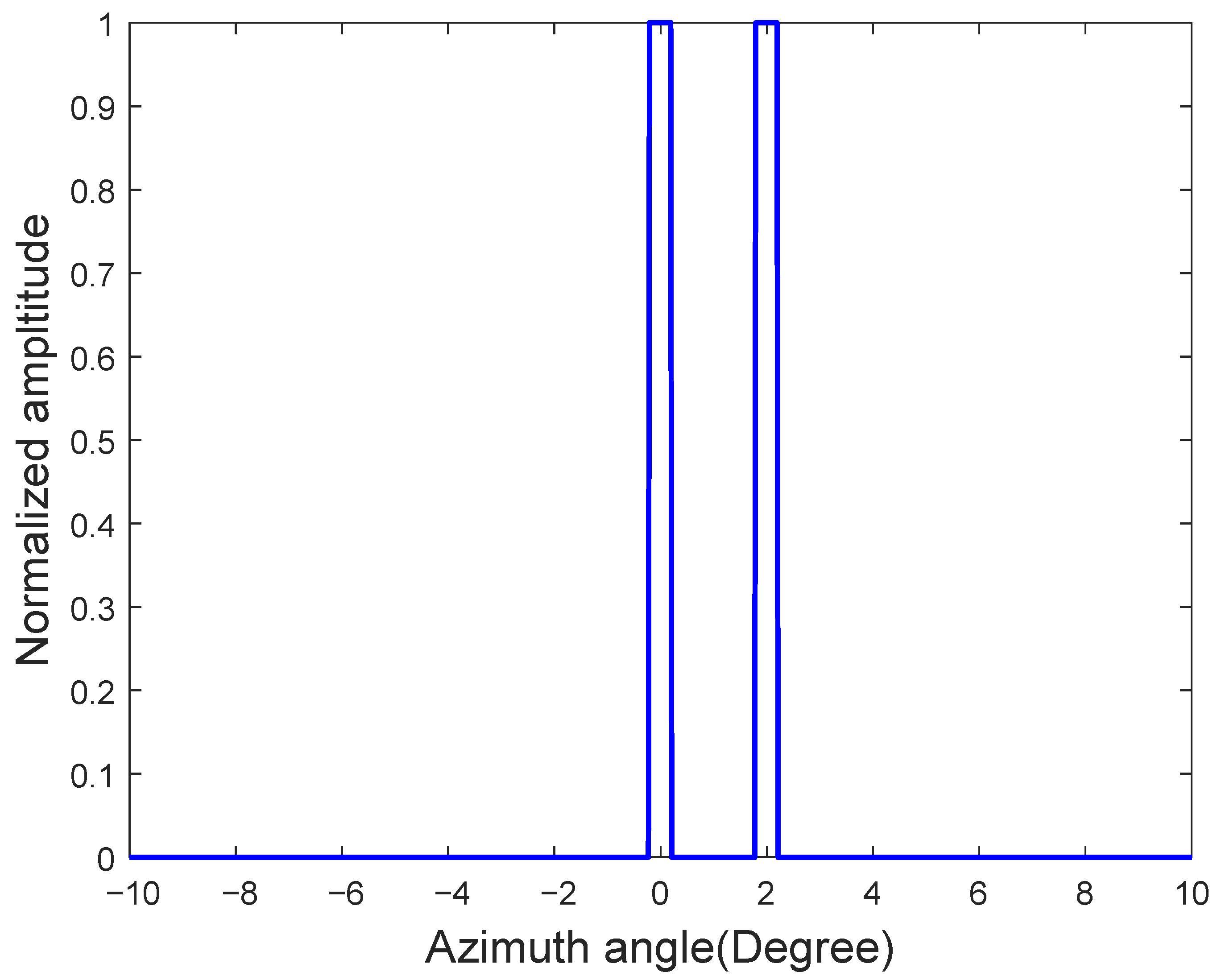
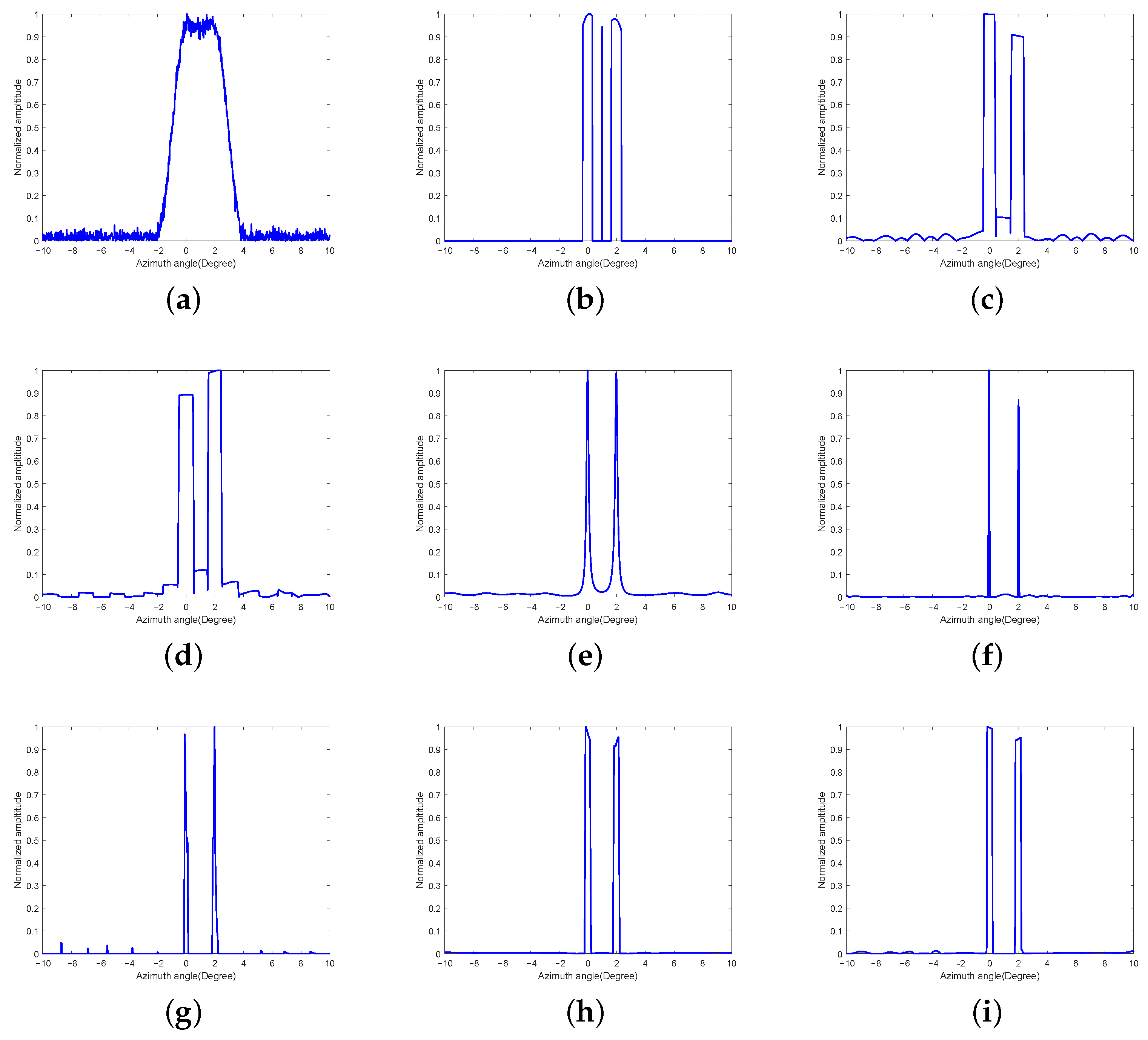
The initial point target configuration is shown in Figure 2, featuring two targets of equal amplitude and edge properties located at $0°$ and $2°$ azimuth positions. Figure 3a displays the received echoes at 25 dB SNR. Beamwidth-induced aliasing occurs due to the target angular separation being smaller than the antenna beamwidth. We conducted 100 Monte Carlo simulation trials, with representative super-resolution processing outcomes demonstrated in Figure 3b–i.

Figure 3b displays the OMP approach ($k=70$, $\nu =100$). Although this method can effectively delineate target contours, its resolution remains limited, and it produces a noticeable false target. Figure 3c presents the reconstruction using conventional TV regularization ($k=70$, $\mu =0.04$, $\gamma =5$), revealing significant sidelobe artifacts and limited resolution capability. Figure 3d displays the online TV reconstruction ($\mu =0.1$, $\gamma =50$), which, similarly to conventional TV regularization, exhibits pronounced sidelobe artifacts and degraded resolution performance. In the simulation environment, while the OMP method demonstrates satisfactory noise suppression performance, it generates distinct reconstruction artifacts. Both TV-based methods exhibit inadequate noise suppression capabilities along with noticeable artifacts in their imaging results.

Figure 3e presents the reconstruction using IAA approach ($k=70$, $\partial =0.1$). It can be seen that this method can distinguish the target well and has a relatively high resolution, but it cannot display the edge information of the target. Figure 3f presents the split SPICE reconstruction ($k=70$, $\gamma =50$), demonstrating superior performance relative to both traditional and online TV methods with markedly suppressed sidelobes and enhanced resolution. However, the technique shows limited capability in preserving target edge delineation. Figure 3g demonstrates the online q-SPICE reconstruction ($q=2$), which achieves comparable performance to the split SPICE approach with substantial sidelobe suppression and resolution enhancement. However, similar limitations persist in accurately representing target edge geometries. In the simulation environment, both SPICE methods and the IAA method demonstrate competent noise suppression performance while maintaining artifact-free reconstruction quality. As can be observed, both SPICE methods demonstrate superior resolution compared to the IAA approach.

The split SPICE-TV method’s output ($k=70$, $\mu =0.04$, ${\gamma }_1=70$, ${\gamma }_2=4$) in Figure 3h reveals significant advancements over previous techniques: while maintaining the sidelobe and resolution advantages of SPICE, it uniquely preserves edge information that was previously obscured. Finally, the imaging result of the grid-updating split SPICE-TV method ($\mu =0.04$, ${\gamma }_1=70$, ${\gamma }_2=4$) is presented in Figure 3i. The sidelobe suppression effect of this proposed method is significantly superior to that of the two TV methods, and it also enhances resolution. In comparison to the split SPICE method and online q-SPICE method, the edge contours of the targets are clearly displayed. Furthermore, the sidelobe suppression and resolution improvement effects are essentially comparable to those of the split SPICE-TV method. In the simulation environment, the imaging results of the two split SPICE-TV methods demonstrate satisfactory noise suppression performance without observable artifacts.

4.1.2. Quantitative Analysis

For comprehensive super-resolution performance assessment, the Relative Error (ReErr) metric is employed to quantify the correlation between reconstructed images and the original scene. The ReErr is mathematically defined as

$$\begin{array}{c}\hfill \mathrm{ReErr}={\displaystyle \frac{{∥\widehat{\mathbf{x}}-\mathbf{x}∥}_2^2}{{∥\mathbf{x}∥}_2^2}}\end{array}$$

(48)

where $\widehat{\mathbf{x}}$ corresponds to the super-resolved reconstruction and $\mathbf{x}$ represents the ground truth. The metric exhibits an inverse relationship with reconstruction fidelity—lower ReErr values indicate superior imaging quality through closer approximation to the original scene.

We conducted 100 Monte Carlo trials, recording the maximum, minimum, and mean values of ReErr along with the average runtime for each method. These performance metrics are comprehensively summarized in

Table 1. Analysis of imaging quality for point target simulation.

Method	ReErr			Runtime
	MIN	MAX	MEAN
OMP Method	$0.617$	$0.628$	$0.622$	$0.099$ s
Traditional TV Method	$0.877$	$0.889$	$0.883$	$1.148$ s
Online TV Method	$0.016$	$0.426$	$0.939$	$0.021$ s
IAA Method	$0.419$	$0.432$	$0.426$	$2.846$ s
Split SPICE Method	$0.789$	$0.801$	$0.795$	$1.514$ s
Online q-SPICE Method	$0.632$	$0.643$	$0.638$	$0.022$ s
Split SPICE-TV Method	$0.061$	$0.076$	$0.070$	$1.293$ s
Proposed Method	$0.062$	$0.077$	$0.071$	$0.029$ s

. Quantitative comparisons at 25 dB SNR are summarized in Table 1. Notably, the ReErr value of the beam-updating split SPICE-TV method is significantly lower than that of the IAA method, the OMP method, the traditional TV method, the online TV method, the split SPICE method, and the online q-SPICE method, while remaining comparable to the split SPICE-TV method.

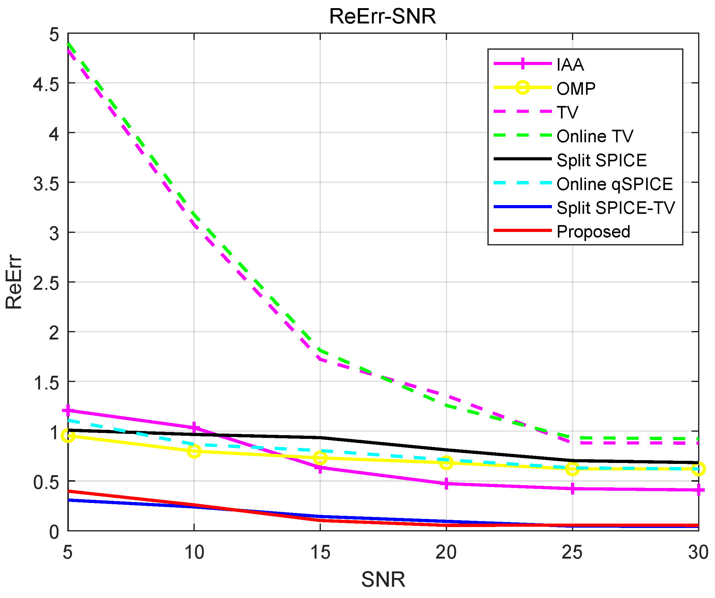
To further analyze the noise suppression performance of each method, Figure 4 illustrates the ReErr variation across SNR levels for all eight approaches, using the parameter configurations specified in Table 1. The proposed approach maintains superior performance (lower ReErr) compared to IAA, OMP, traditional TV, online TV, split SPICE, and online q-SPICE methods across all tested SNR conditions, while achieving comparable accuracy to the split SPICE-TV baseline.

The runtime of the eight methods is detailed in Table 1. The proposed method, which does not require matrix inversions during its iterative process, exhibits significantly lower computational complexity compared to batch processing methods. It is clear that the runtime of the proposed method is considerably less than that of the IAA method, the OMP method, the traditional TV method, the split SPICE method, and the split SPICE-TV method. Additionally, its runtime is nearly identical to that of the online TV method and the online q-SPICE method, consistent with the earlier theoretical analysis.

4.2. Surface Target Simulation

This section presents a surface target simulation to rigorously evaluate the grid-updating split SPICE-TV method’s efficacy. The complete simulation configuration is specified in

Table 2. Simulation parameters of the surface target.

Parameter	Value
Beam width	$4°$
Scanning region	$-20°\sim 20°$
Scanning speed	$100°$/s
PRF	$1000$ Hz
Carrier Frequency	$10$ GHz
Bandwidth	$45$ MHz
Time width	$1 \mu \mathrm{s}$
Sampling Frequency	$90$ MHz

.

4.2.1. Surface Target Results

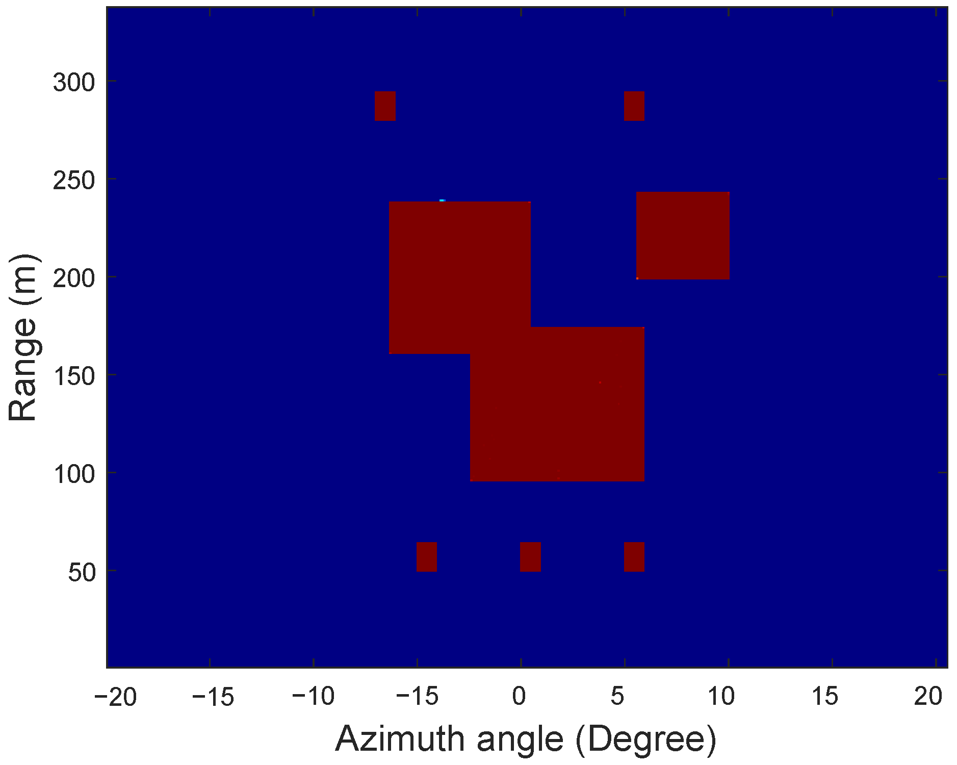
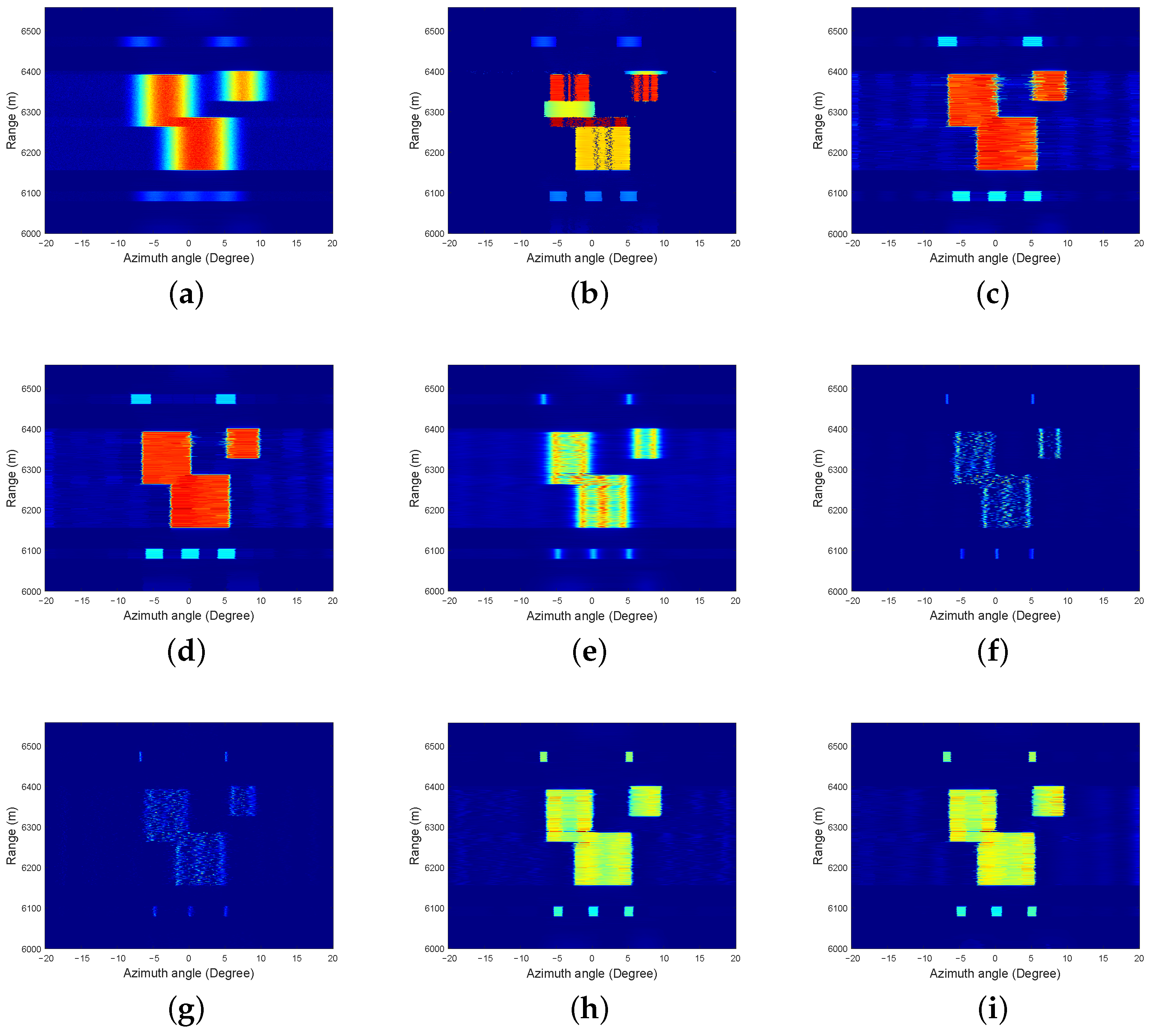
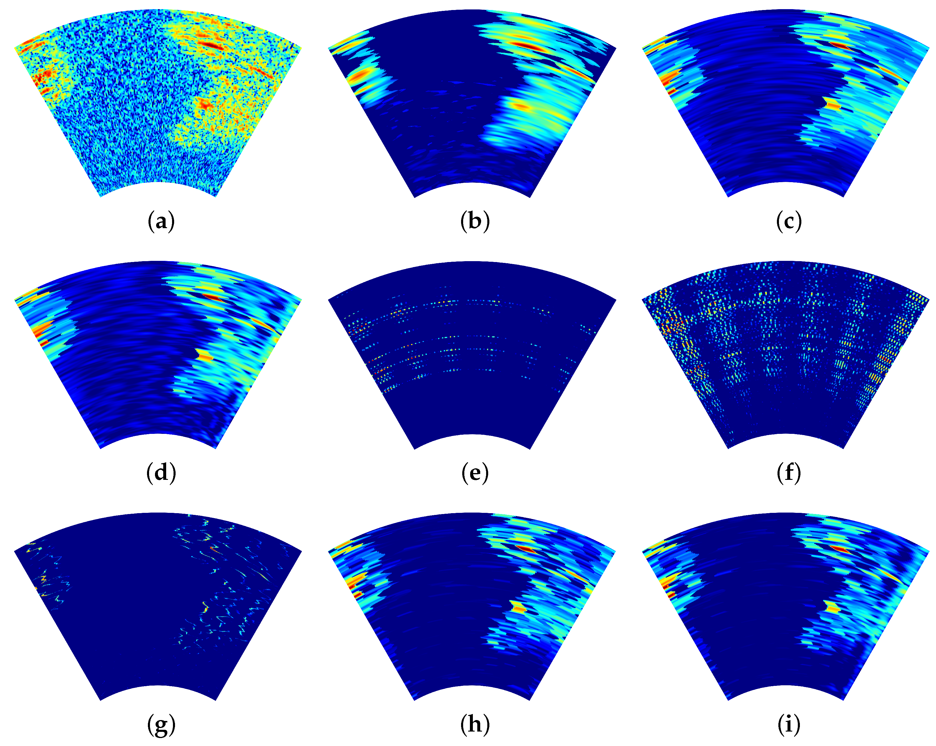
Figure 5 displays the reference surface target scenario, consisting of three rectangular landmasses. Two connected islands contain five sparse targets in total—two positioned above and three below. The 20 dB SNR echo response in Figure 6a shows beamwidth-induced overlap among the lower three targets due to insufficient angular separation. Across 100 Monte Carlo simulation trials, representative super-resolution processing outcomes are demonstrated in Figure 6b–i, with all parameters consistent with the point target simulation protocol.

The simulation result of the OMP method is presented in Figure 6b. It can be seen that the resolution of this method is relatively low and it cannot restore the outline of the extended island target very well. The simulation result of the traditional TV method is shown in Figure 6c. Similar to the point target simulation results, this method exhibits numerous sidelobes and demonstrates lower resolution for the five sparse targets above and below. The simulation result of the online TV method is presented in Figure 6d. Analysis reveals that the five sparse targets exhibit very low resolution, with noticeable sidelobes present in the center of the island target. While the OMP method demonstrates satisfactory noise suppression performance, it generates distinct reconstruction artifacts. Both TV-based methods exhibit inadequate noise suppression capabilities along with noticeable artifacts in their imaging results.

The simulation result of the IAA method is shown in Figure 6e. Although the imaging result of this method has a very high resolution, the peaks and troughs can be clearly seen from the imaging result of the intermediate extended island targets. The simulation result of the split SPICE method is shown in Figure 6f. While this method achieves high resolution for the five sparse targets, it fails to capture the edge characteristics of the targets and does not identify the intermediate island targets. The simulation result of the online q-SPICE method is displayed in Figure 6g. Although the resolution of the five sparse targets is high, it does not accurately represent the outline of the middle island target. Both SPICE methods and the IAA method demonstrate competent noise suppression performance while maintaining artifact-free reconstruction quality. As can be observed, both SPICE methods demonstrate superior resolution compared to the IAA approach.

The simulation result of the split SPICE-TV method is shown in Figure 6h. Compared to the traditional TV method and the online TV method, the split SPICE-TV method reduces sidelobes of the island group targets while enhancing the resolution of the five sparse targets. In contrast to the split SPICE method and the online q-SPICE method, this approach effectively captures the edge contours of the targets. The imaging results of the grid-updating split SPICE-TV method are illustrated in Figure 6i. It is evident that the proposed method outperforms the traditional TV method and the online TV method in terms of resolution and sidelobe suppression. Furthermore, in comparison to the split SPICE method and the online q-SPICE method, the proposed approach accurately identifies island targets and reflects target contours, with imaging results largely consistent with those of the split SPICE-TV method. The imaging results of the two split SPICE-TV methods demonstrate satisfactory noise suppression performance without observable artifacts.

4.2.2. Quantitative Analysis

For quantitative super-resolution assessment of the Figure 6 results, we utilize the Structural Similarity Index (SSIM) to measure the reconstruction fidelity. SSIM comprehensively evaluates the perceptual image quality through luminance, contrast, and structural comparisons, with values approaching one indicating optimal reconstruction. The metric is mathematically defined as

$$\begin{array}{c}\hfill \begin{array}{c}\mathrm{SSIM}(\mathbf{X},\mathbf{Y})={\displaystyle \frac{\left(2u_{\mathbf{X}}{u}_{\mathbf{Y}}+c_1\right)\left(2{\delta }_{\mathbf{XY}}+c_2\right)}{\left(u_{\mathbf{X}}^2+u_{\mathbf{Y}}^2+c_1\right)\left({\delta }_{\mathbf{X}}^2+{\delta }_{\mathbf{Y}}^2+c_2\right)}}\end{array}\end{array}$$

(49)

where $\mathbf{X}$ is the matrix of the results of each super-resolution method, $\mathbf{Y}$ is the echo matrix, ${\mu }_{\mathbf{X}}$ is the average value of $\mathbf{X}$, $u_{\mathbf{Y}}$ is the mean value of $\mathbf{Y}$, ${\delta }_{\mathbf{X}}$ is the variance of $\mathbf{X}$, $u_{\mathbf{Y}}$ is the variance of $\mathbf{Y}$, and $o_{\mathbf{XY}}$ is the covariance of $\mathbf{X}$ and $\mathbf{Y}$.

One hundred Monte Carlo experiments were performed to evaluate each method’s SSIM (maximum, minimum, mean) and average runtime, with the results compiled in

Table 3. Analysis of imaging quality for surface target simulation.

Method	SSIM			Runtime
	MIN	MAX	MEAN
OMP Method	$0.516$	$0.557$	$0.534$	$7.235$ s
Traditional TV Method	$0.675$	$0.714$	$0.693$	$87.725$ s
Online TV Method	$0.672$	$0.711$	$0.695$	$1.997$ s
IAA Method	$0.754$	$0.796$	$0.773$	$237.124$ s
Split SPICE Method	$0.487$	$0.521$	$0.501$	$95.655$ s
Online q-SPICE Method	$0.474$	$0.519$	0.496	$2.004$ s
Split SPICE-TV Method	$0.691$	$0.731$	$0.712$	$90.832$ s
Proposed Method	$0.694$	$0.728$	$0.719$	$2.059$ s

. The SSIM values of the simulation results of the three super-resolution methods are shown in Table 3.

Although the IAA method achieves the highest SSIM value, it exhibits inferior edge recovery performance for extended targets compared to the proposed method, along with significantly higher computational time. The SSIM value of the proposed method is higher than those of the OMP method, traditional TV method, the online TV method, the split SPICE method, and the online q-SPICE method, while remaining nearly identical to that of the split SPICE-TV method.

The runtime of the four methods is presented in Table 3. The computational complexity of the proposed method is significantly lower than that of batch processing methods, as its iterative process does not require matrix inversions. The runtime of the grid-updating split SPICE-TV method is considerably less than that of the IAA method, the OMP method, the traditional TV method, the split SPICE method, and the split SPICE-TV method. Furthermore, it is nearly equivalent to the runtimes of the online TV method and the online q-SPICE method, supporting the earlier theoretical analysis.

The data presented above demonstrate that the proposed method effectively reduces computational complexity while maintaining the high image quality characteristic of the split SPICE-TV method.

4.3. Statistical Significance Analysis

To statistically validate whether the observed differences between ReErr and SSIM metrics in the quantitative analysis are significant rather than coincidental, we conducted a samples t-test for rigorous significance testing. Since ReErr and SSIM are derived from two distinct datasets, we employed an independent samples t-test for statistical validation, which can be formally expressed as

$$\begin{array}{c}\hfill t-test={\displaystyle \frac{{\overline{x}}_{\mathrm{ReErr}}-{\overline{x}}_{\mathrm{SSIM}}}{\sqrt{\frac{s_{\mathrm{ReErr}}^2}{n_{\mathrm{ReErr}}}+\frac{s_{\mathrm{SSIM}}^2}{n_{\mathrm{SSIM}}}}}}\end{array}$$

(50)

where ${\overline{x}}_{\mathrm{ReErr}}$ is the mean of ReErr, ${\overline{x}}_{\mathrm{SSIM}}$ is the mean of SSIM, $s_{\mathrm{ReErr}}^2$ is the variance of ReErr, $s_{\mathrm{SSIM}}^2$ is the variance of SSIM, $n_{\mathrm{ReErr}}$ is the number of Monte Carlo experiments conducted to collect ReErr, and $n_{\mathrm{SSIM}}$ is the number of Monte Carlo experiments conducted to collect SSIM. We have conducted 100 Monte Carlo simulations to evaluate the proposed method’s ReErr and SSIM performance metrics, followed by rigorous t-test statistical analysis. The statistical analysis yielded $t-test=1.005$ ($p=0.328$), indicating no significant difference at the $\alpha =0.05$ level.

5. Measured Data Results

In the previous section, the feasibility of the proposed method was demonstrated through point target and surface target simulations. To further evaluate the imaging performance of the grid-updating split SPICE-TV method, this section processes two sets of measured data using the IAA method, the OMP method, the traditional TV method, the online TV method, the split SPICE method, the online q-SPICE method, the split SPICE-TV method, and the grid-updating split SPICE-TV method to validate the restoration capabilities of the grid-updating split SPICE-TV method for sparse targets and target contours. Additionally, a prominent point was selected in the scene, and profiles of the echoes, along with results from the IAA method, the OMP method, the traditional TV method, the online TV method, the split SPICE method, the online q-SPICE method, the split SPICE-TV method, and the grid-updating split SPICE-TV method, were compared.

5.1. Imaging for Urban Monitoring Applications

In this section, the effectiveness of the proposed method is validated using measured data collected from a urban monitoring application. The experimental parameters are presented in

Table 4. Experimental parameters.

Parameter	Value
Carrier frequency	X band
Scanning range	$-180°\sim 180°$
Scanning speed	$24{}^{\circ }/\mathrm{s}$
Beamwidth	$5.1°$
PRF	$200$ Hz
Platform velocity	$0$ m/s
Platform height	$3$ m
Pitch angle	$10°$

.

5.1.1. Imaging Results

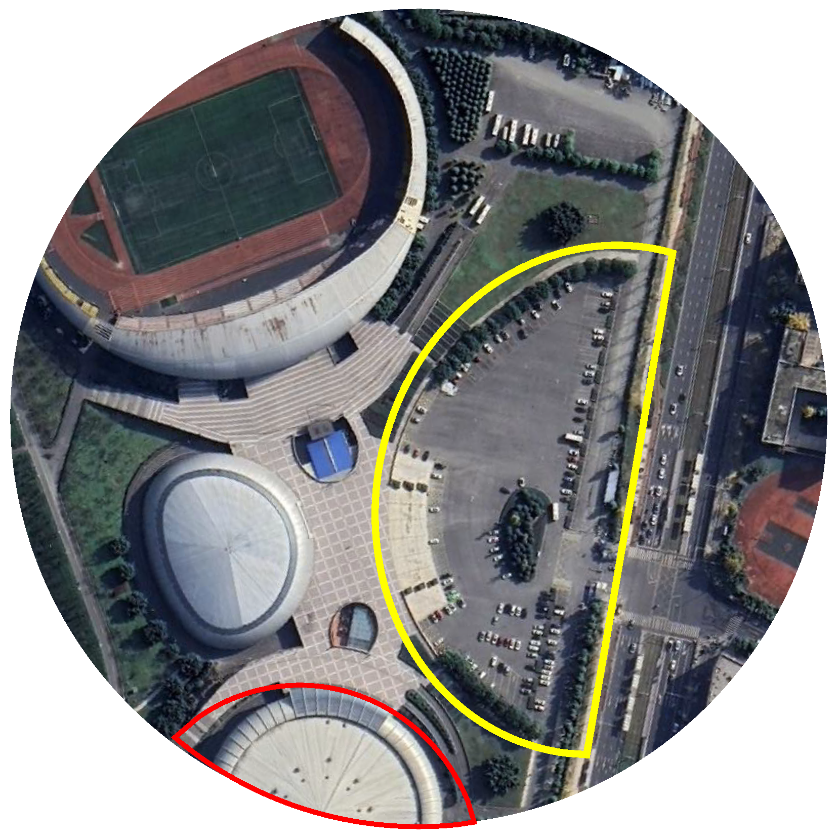
The real scene is depicted in Figure 7, where the building outlined in red and the parking lot marked in yellow represent the key areas of interest for this set of measured data. The echo pattern of the original scene, shown in Figure 8a, demonstrates clear contours in both the red and yellow regions. The super-resolution imaging results are presented in Figure 8b–i. All methodological parameters maintain identical configurations to those implemented in the previous section.

The imaging result of the OMP method is shown in Figure 8b. The results indicate no significant resolution improvement compared to the original echo data. The imaging result of the traditional TV method is displayed in Figure 8c. Compared to the echo of the original scene, the contours of the imaging results in the red and yellow regions are sharper, but the improvement in resolution is limited. The imaging result of the online TV method is shown in Figure 8d. Similar to the traditional TV method, the imaging results of the online TV method exhibit sharper contours in the red and yellow regions. However, the enhancement in the azimuth resolution remains minimal. Consistent with the favorable simulation results obtained previously, the OMP method and two TV methods demonstrate comparably effective noise suppression performance with artifacts under high-SNR experimental conditions.

The imaging result of the IAA method is displayed in Figure 8e. As observed, the IAA method suffers from severe energy dispersion and sidelobe interference when dealing with complex scenes, significantly degrading its resolution performance. The imaging result of the split SPICE method is presented in Figure 8f. It can be observed that, although the split SPICE method demonstrates a significant improvement in azimuth resolution compared to both the traditional TV method and the online TV method, this approach fails to reconstruct the contours of the building in the red region and the parking lot in the yellow region. The imaging result of the q-SPICE method is shown in Figure 8g. Similar to the split SPICE method, despite its high resolution, this method fails to reveal the contours of the targets in the red and yellow regions. Diverging from the favorable simulation outcomes, high-SNR experimental measurements reveal marked performance differences: the IAA method demonstrates substantially degraded noise suppression with conspicuous artifacts, whereas both SPICE variants maintain excellent noise rejection capabilities while producing artifact-free reconstructions.

The imaging result of the split SPICE-TV method is displayed in Figure 8h. Compared to the traditional TV method and the online TV method, the split SPICE-TV method significantly enhances the resolution of targets in both the red and yellow regions. Furthermore, in contrast to the split SPICE method and the online q-SPICE method, the split SPICE-TV method successfully reconstructs the contours of the targets in the red and yellow regions. The imaging result of the grid-updating split SPICE-TV method is shown in Figure 8i. It is also evident that the proposed method significantly improves the resolution of targets in the red and yellow regions compared to the traditional TV method and the online TV method. Additionally, it successfully reconstructs the contours of the targets in these regions, outperforming both the split SPICE method and the online q-SPICE method. Moreover, the imaging result is nearly identical to that of the split SPICE-TV method. Under high-SNR measured data conditions, the imaging results of the two split SPICE-TV methods exhibit superior noise suppression performance while remaining entirely free of discernible artifacts.

5.1.2. Quantitative Analysis

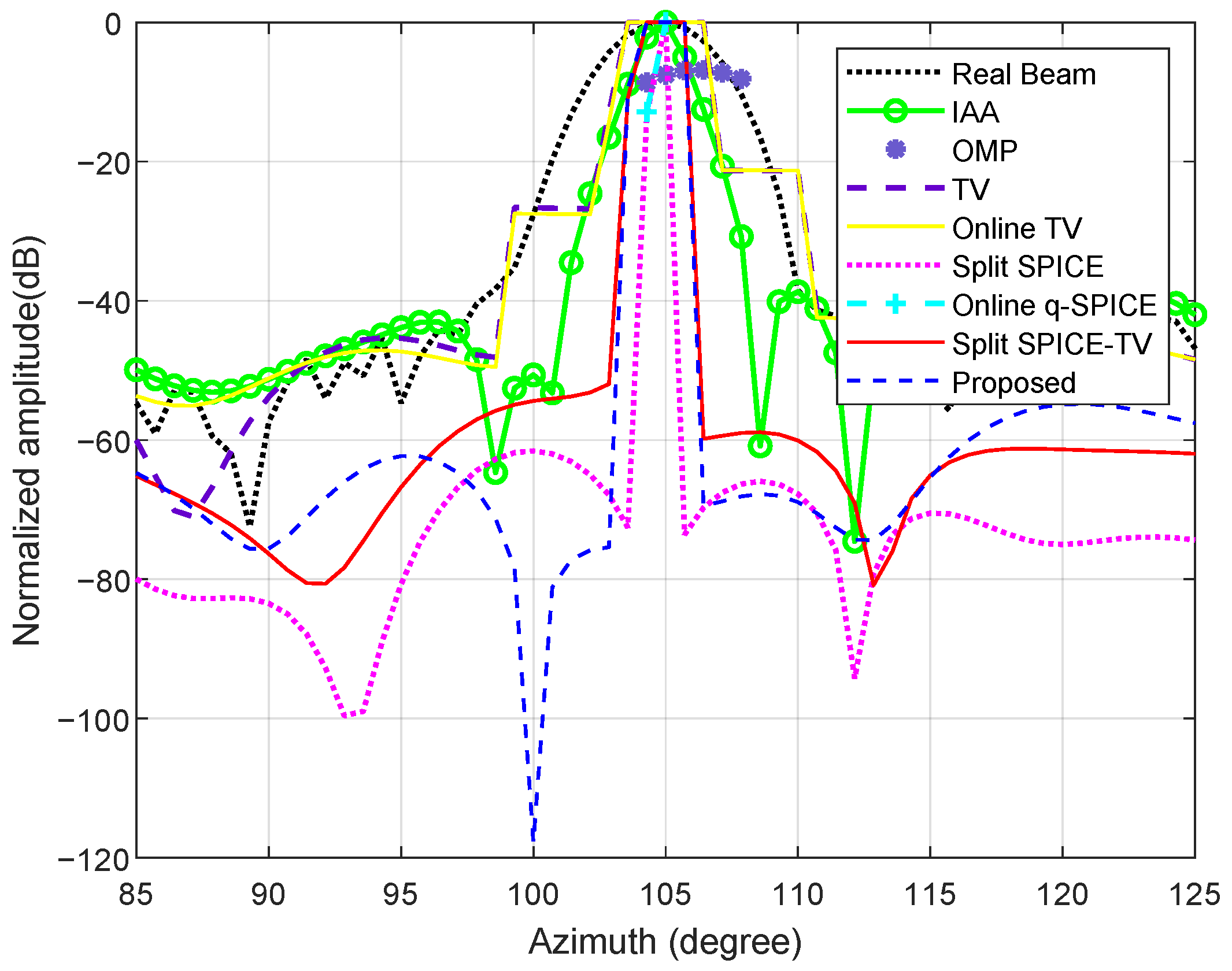
The range bin of 50 m from the profile results of the eight methods is extracted from Figure 8 and depicted in Figure 9. As demonstrated, when processing complex real-world scenarios, both IAA and OMP methods exhibit significantly lower resolution performance compared to the proposed approach. In comparison to the traditional TV method and the online TV method, the proposed method exhibits reduced sidelobes and enhanced resolution. Additionally, when compared to the online q-SPICE method, it successfully recovers the target contours, yielding imaging results similar to those of the split SPICE-TV method.

Table 5. Analysis of imaging quality for measured data.

Method	−3 dB Bandwidths	Runtime
OMP Method	$3.571$	$2.086$ s
Traditional TV Method	$2.858$	$52.311$ s
Online TV Method	$2.859$	$0.007$ s
IAA Method	$2.143$	$81.281$ s
Split SPICE Method	$0.928$	$56.363$ s
Online q-SPICE Method	$0.931$	$0.008$ s
Split SPICE-TV Method	$1.428$	$54.314$ s
Proposed Method	$1.430$	$0.008$ s

compares the −3 dB bandwidth performance across methods. The proposed method demonstrates superior resolution (narrower bandwidth) to the IAA method, the OMP method, the traditional TV method, the online TV method while matching the split SPICE-TV’s performance. The proposed method outperforms both TV variants and maintains comparable bandwidth characteristics to split SPICE-TV.

The runtime of the eight methods is presented in Table 5. The runtime of the grid-updating split SPICE-TV method is significantly shorter than that of the IAA method, the OMP method, the traditional TV method, the split SPICE method, and the split SPICE-TV method, while remaining nearly the same as that of the online TV method and the online q-SPICE method, which aligns with the earlier theoretical analysis.

5.2. Imaging for Coastal Monitoring Applications

In the previous section, the effectiveness of the proposed method was demonstrated using measured data recorded from a urban monitoring application. In this section, measured data captured from a coastal monitoring application will be utilized to further validate the efficacy of the proposed method. The experimental parameters are detailed in

Table 6. Experimental parameters.

Parameter	Value
Carrier frequency	X band
Scanning range	$-30°\sim 30°$
Scanning speed	$72{}^{\circ }/\mathrm{s}$
Beamwidth	$5.1°$
PRF	$200$ Hz
Platform velocity	$47$ m/s
Platform height	$300$ m
Pitch angle	$30°$

.

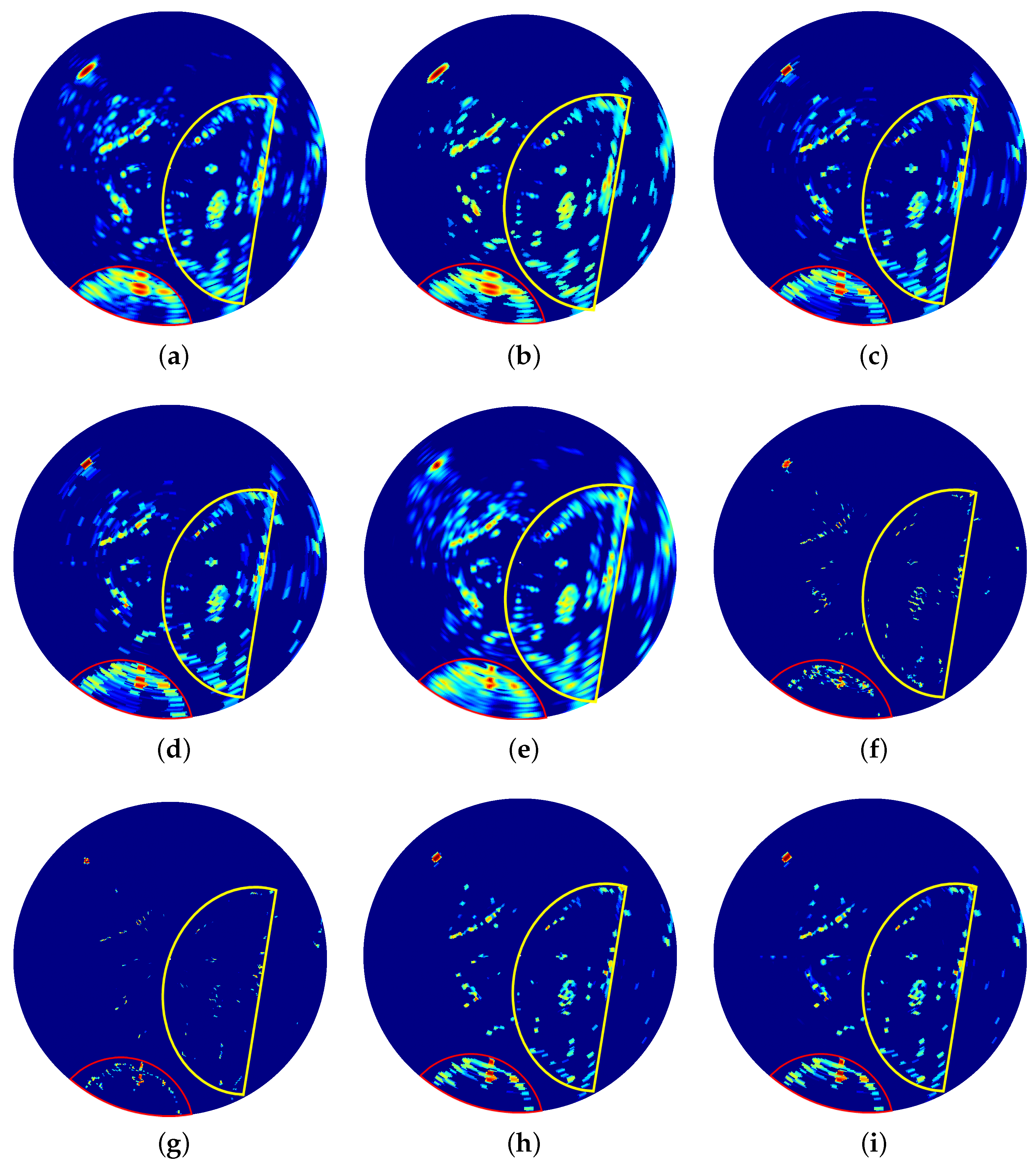
The real scene is depicted in Figure 10, where two outlined targets are visible in the bottom-left and top-right corners. The echo of the original scene is shown in Figure 11a. The super-resolution imaging results are illustrated in Figure 11b–i. Due to the high level of noise present in the measured data, the parameters of the methods discussed in the preceding sections are not directly applicable here. Consequently, the parameters for each method have been re-adjusted in this section to accommodate the specific characteristics of the measured data.

The imaging result of the OMP method ($k=70$, $\nu$ = 10,000) is shown in Figure 11b. Similar to the previous set of measured data result obtained with the OMP method, the imaging resolution shows no significant improvement. The imaging result of the traditional TV method ($k=70$, $\mu$ = 20,000, $\gamma =50$) is displayed in Figure 11c, which contains numerous sidelobes. The imaging result of the online TV method ($\mu$ = 20,000, $\gamma =10$) is shown in Figure 11d. Similar to the traditional TV method, the online TV method also exhibits sidelobes. Under low-SNR experimental conditions, the imaging results of the above three methods demonstrate adequate noise suppression performance while exhibiting moderate artifact levels.

The imaging result of the IAA method ($k=70$, $\partial =1000$) is displayed in Figure 11e. As evidenced by the results, the IAA method demonstrates significantly degraded imaging performance when processing complex scenes with severe background noise. The imaging result of the split SPICE method ($k=70$, $\gamma$ = 10,000) is presented in Figure 11f. Due to significant noise in the echoes, the split SPICE method is unable to identify the edges of the targets. The imaging result of the q-SPICE method ($q=2$) is shown in Figure 11g. Despite its high resolution, this method fails to reveal the contours of the targets. Under low-SNR experimental conditions, both IAA and split SPICE methods exhibit substantially compromised noise suppression capabilities along with clearly visible artifacts. In contrast, the online q-SPICE method maintains robust noise rejection performance while producing artifact-free reconstructions.

The imaging result of the split SPICE-TV method ($k=70$, $\mu$ = 10,000, ${\gamma }_1=70$, ${\gamma }_2=4$) is displayed in Figure 11h, where a decrease in the number of sidelobes and an increase in resolution can be observed. The imaging result of the grid-updating split SPICE-TV method ($\mu$ = 10,000, ${\gamma }_1=100$, ${\gamma }_2=40$) is shown in Figure 11i. Similarly, it can be observed that its sidelobes are smaller than those of the traditional TV method and the online TV method, and it exhibits higher resolution compared to both. The imaging result is nearly identical to that of the split SPICE-TV method. Under low-SNR measured data conditions, the imaging results of the two split SPICE-TV methods maintain competent noise suppression performance while exhibiting no discernible artifacts.

Table 7. Runtime for measured data.

Method	Runtime
OMP Method	$2.881$ s
Traditional TV Method	$76.556$ s
Online TV Method	$0.597$ s
IAA Method	$126.611$ s
Split SPICE Method	$82.812$ s
Online q-SPICE Method	$0.604$ s
Split SPICE-TV Method	$79.641$ s
Proposed Method	$0.657$ s

presents the runtime of all evaluated methods. The runtime of the grid-updating split SPICE-TV method is significantly shorter than that of the IAA method, the OMP method, the traditional TV method, the split SPICE method, and the split SPICE-TV method, while remaining nearly identical to that of the online TV method and the online q-SPICE method, consistent with the earlier theoretical analysis.

The above analysis demonstrates that the proposed method effectively reduces computational complexity while preserving the high image quality of the split SPICE-TV method.

6. Conclusions

In this paper, we introduce an grid-updating split SPICE-TV method tailored for scanning radars. This method boasts several advantages. Firstly, compared to the traditional SPICE approach, it integrates TV norm regularization, better preserving azimuthal edge contours. In contrast to conventional TV regularization methods, our approach yields higher imaging resolution and lower sidelobes. Secondly, unlike traditional online methods with a single constraint term, our proposed method incorporates two constraint terms, facilitating the recovery of both sparse targets and edge contours simultaneously. Lastly, in comparison to the existing methods based on Bregman iteration, our proposed approach offers an online closed-form solution, significantly reducing computational costs without compromising imaging quality. Simulation and experimental validations substantiate the effectiveness of the proposed method.

However, the practical deployment of the proposed method is constrained by its requirement for the manual adjustment of three critical parameters. The performance degrades when these parameters are mismatched to dynamic operational environments (e.g., varying clutter or SNR conditions), and the manual tuning process reduces reproducibility across different radar systems. To address these limitations, our future work will focus on developing a neural network architecture capable of predicting optimal parameters directly from raw radar data. This adaptive parameter selection approach would preserve the method’s theoretical advantages while eliminating its manual tuning bottleneck, thereby facilitating real-world field applications.