
A Dual-Variable Selection Framework for Enhancing Forest Aboveground Biomass Estimation via Multi-Source Remote Sensing

 , , ,
, , ,
Abstract
1. Introduction
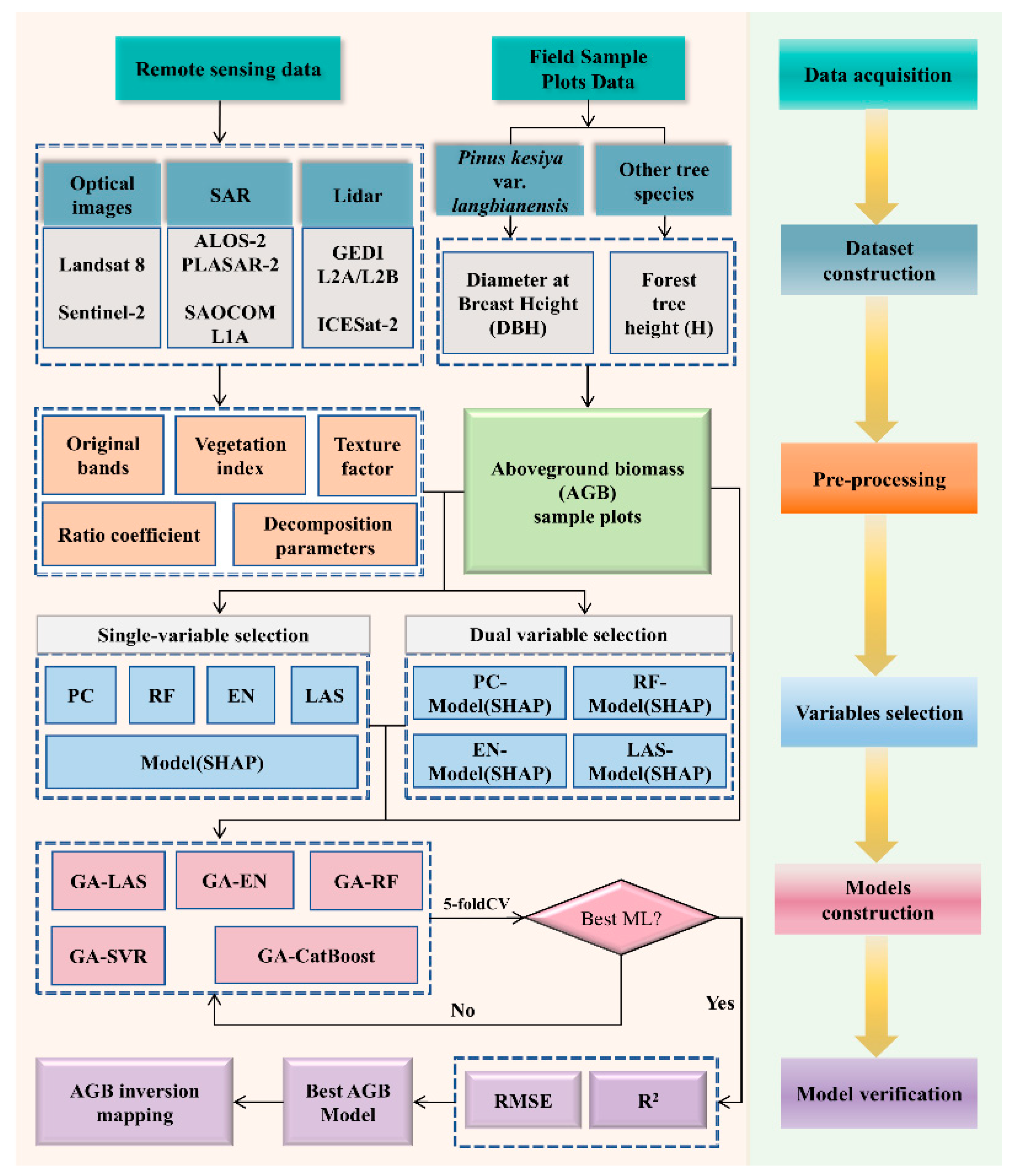
2. Methods
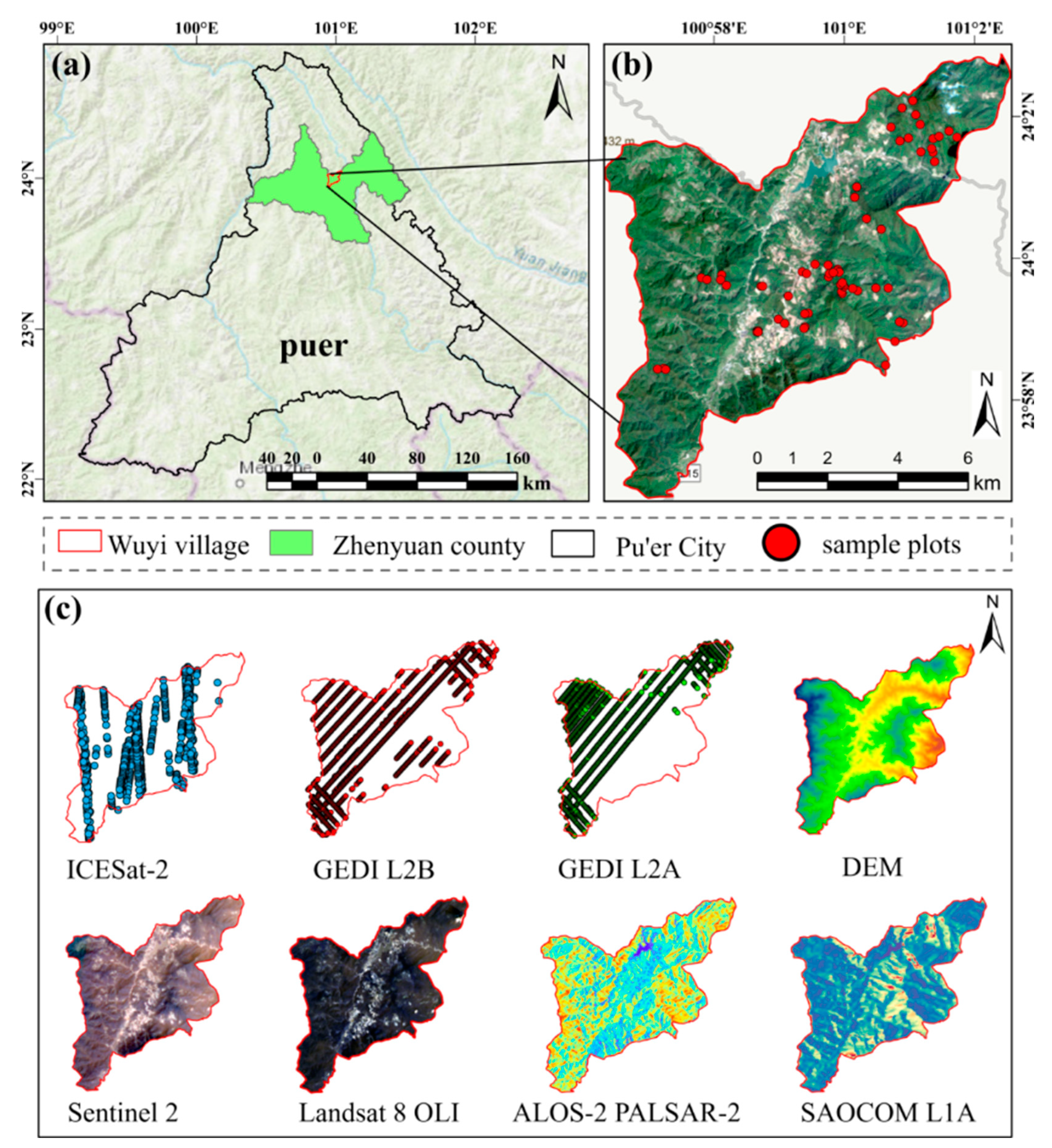
2.1. Study Area
2.2. Data Acquisition and Processing
2.2.1. Sample Plot Collection and Forest AGB Estimation
2.2.2. Multi-Source Geospatial and Remote Sensing Datasets
2.2.3. Remote Sensing Variable Extraction
2.3. Variable Selection Methods
2.4. AGB Model Parameter Optimization
2.5. Model Evaluation
3. Analysis of Results
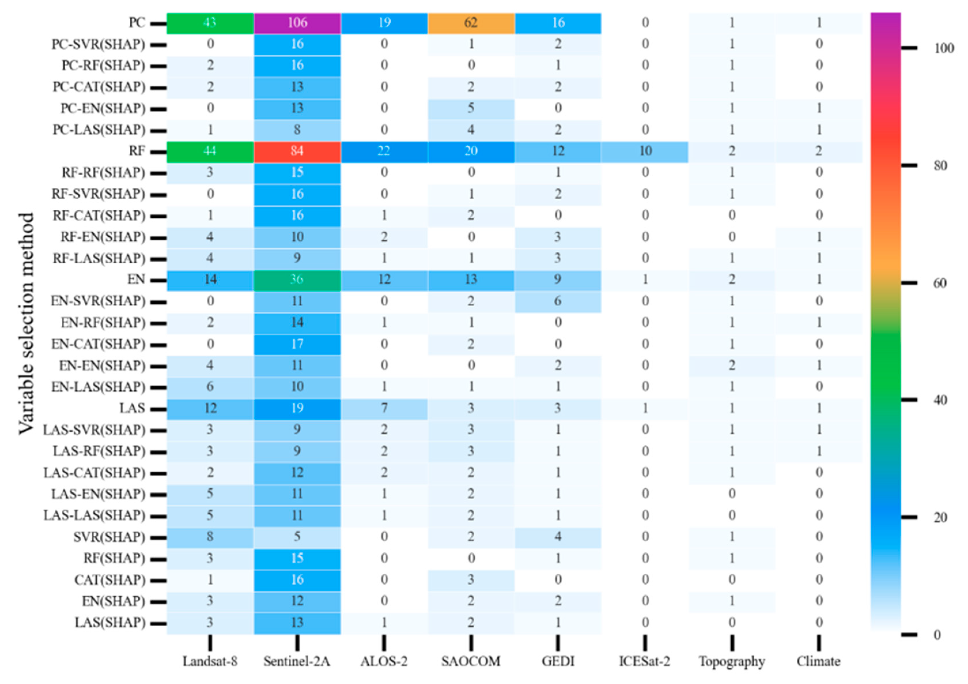
3.1. Model Variable Selection
3.2. Model Results Analysis
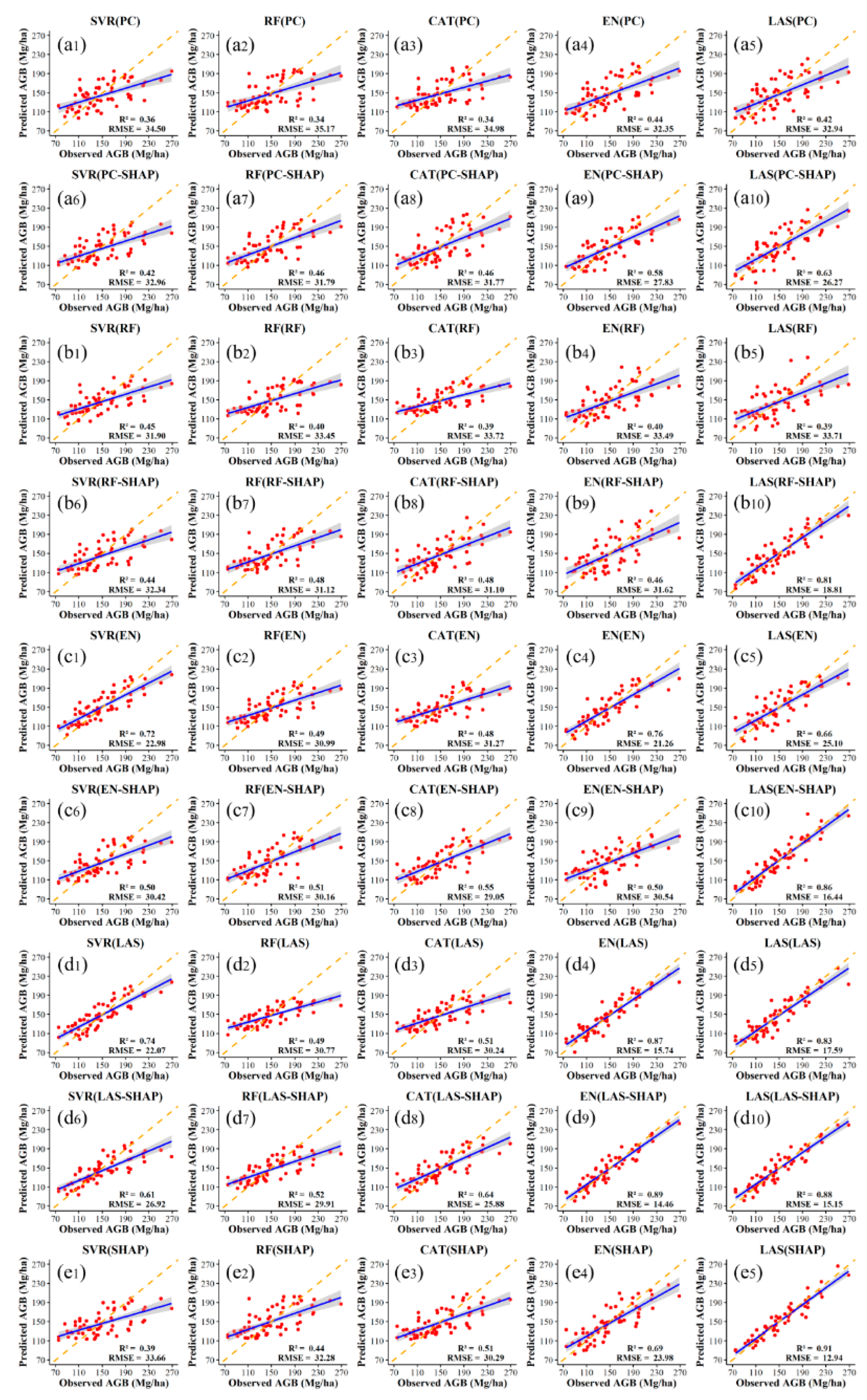
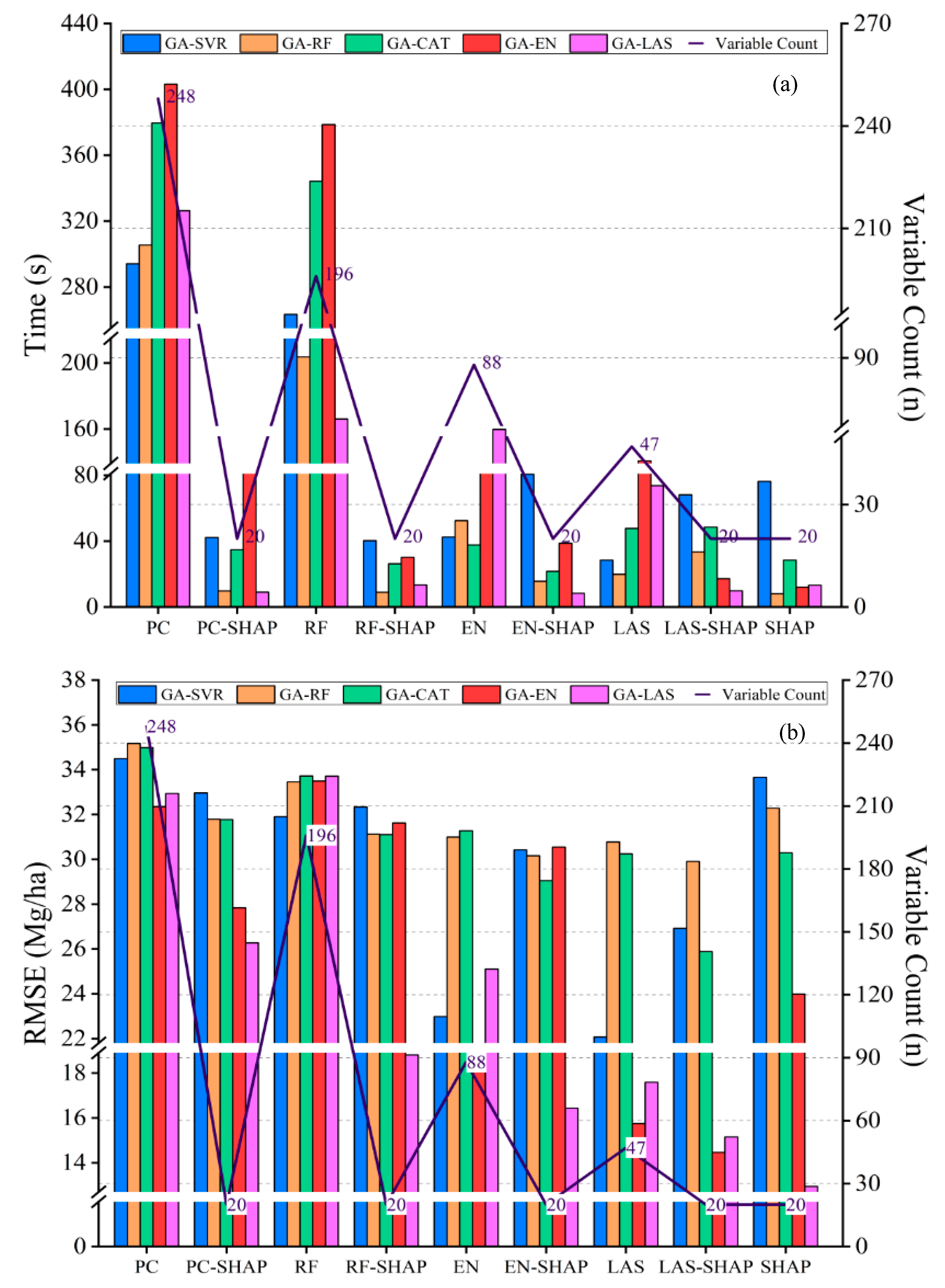
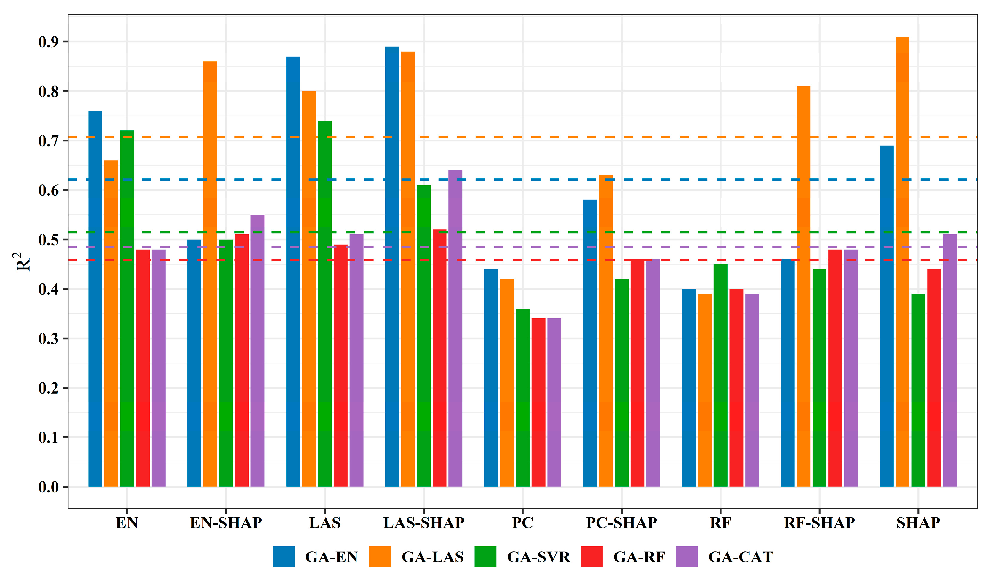
3.2.1. Comparison of AGB Estimation Accuracy Across Different Variable Selection Methods
3.2.2. Comparison of the Accuracy for the Five Models
3.2.3. Comparison of Variable Selection Differences Among Models
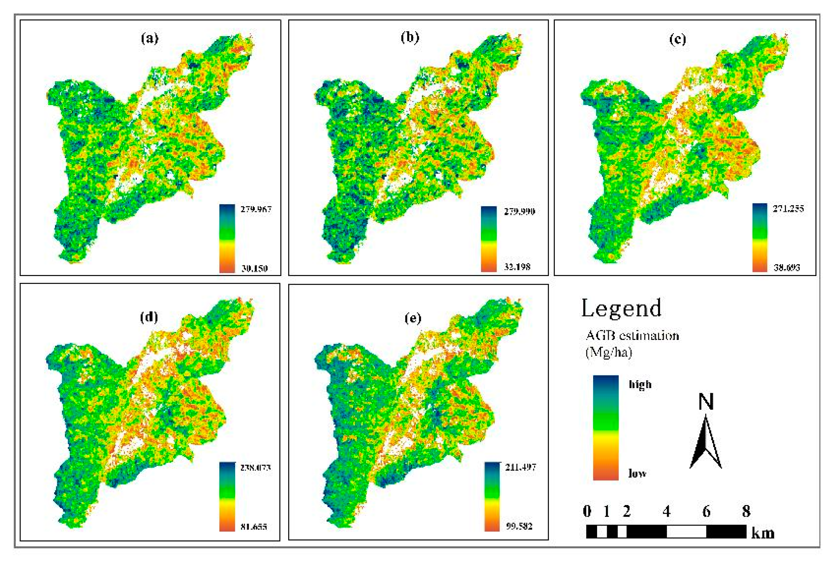
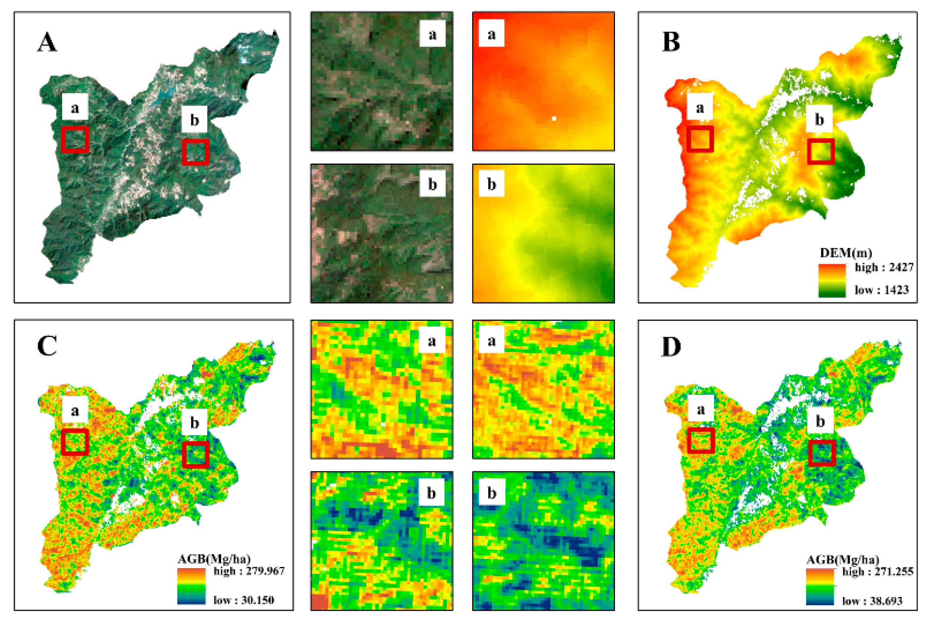
3.3. Comparison of AGB Inversion Across Different Models
4. Discussion
4.1. Contribution of Dual-Variable Selection to Enhancing AGB Estimation Accuracy
4.2. Impact of Estimation Model Selection on AGB Estimation
4.3. Variations in Optimal AGB Estimation Among Models
4.4. Limitations and Future Perspectives
5. Conclusions
Author Contributions
Funding
Data Availability Statement
Conflicts of Interest
References
- Antonarakis, A. Linking carbon and water cycles with forests. Geography 2018, 103, 4–11. [Google Scholar] [CrossRef]
- Fujii, H.; Sato, M.; Managi, S. Decomposition Analysis of Forest Ecosystem Services Values. Sustainability 2017, 9, 687. [Google Scholar] [CrossRef]
- Zhang, Y.; Liang, S. Fusion of Multiple Gridded Biomass Datasets for Generating a Global Forest Aboveground Biomass Map. Remote Sens. 2020, 12, 2559. [Google Scholar] [CrossRef]
- Yang, C.; Sun, W.; Zhu, J.; Ji, C.; Feng, Y.; Ma, S.; Shi, Y.; Guo, Z.; Fang, J. Updated estimation of forest biomass carbon pools in China, 1977–2018. Biogeosci. Discuss. 2022, 19, 2989–2999. [Google Scholar] [CrossRef]
- Yang, H.; Qin, Z.; Shu, Q.; Xu, L.; Yu, J.; Luo, S.; Wu, Z.; Xia, C.; Yang, Z. Estimation of Above-ground Biomass for Dendrocalamus giganteus Utilizing Spaceborne LiDAR GEDI Data. IEEE J. Sel. Top. Appl. Earth Obs. Remote Sens. 2025, 18, 5271–5286. [Google Scholar] [CrossRef]
- Ge, J.; Hou, M.; Liang, T.; Feng, Q.; Meng, X.; Liu, J.; Bao, X.; Gao, H. Spatiotemporal dynamics of grassland aboveground biomass and its driving factors in North China over the past 20 years. Sci. Total Environ. 2022, 826, 154226. [Google Scholar] [CrossRef]
- Zhang, R.; Zhou, X.; Ouyang, Z.; Avitabile, V.; Qi, J.; Chen, J.; Giannico, V. Estimating aboveground biomass in subtropical forests of China by integrating multisource remote sensing and ground data. Remote Sens. Environ. 2019, 232, 111341. [Google Scholar] [CrossRef]
- Lu, D. The potential and challenge of remote sensing-based biomass estimation. Int. J. Remote Sens. 2006, 27, 1297–1328. [Google Scholar] [CrossRef]
- Pertille, C.T.; Nicoletti, M.F.; Topanotti, L.R.; Stepka, T.F. Biomass quantification of Pinus taeda L. from remote optical sensor data. Adv. For. Sci. 2019, 6, 603–610. [Google Scholar] [CrossRef]
- Madundo, S.D.; Mauya, E.W.; Kilawe, C.J. Comparison of multi-source remote sensing data for estimating and mapping above-ground biomass in the West Usambara tropical montane forests. Sci. Afr. 2023, 21, e01763. [Google Scholar] [CrossRef]
- Quang, N.H.; Quinn, C.H.; Carrie, R.; Stringer, L.C.; Van Hue, L.T.; Hackney, C.R.; Van Tan, D. Comparisons of regression and machine learning methods for estimating mangrove above-ground biomass using multiple remote sensing data in the red River Estuaries of Vietnam. Remote Sens. Appl. Soc. Environ. 2022, 26, 100725. [Google Scholar] [CrossRef]
- Kašpar, V.; Hederová, L.; Macek, M.; Müllerová, J.; Prošek, J.; Surový, P.; Wild, J.; Kopecký, M. Temperature buffering in temperate forests: Comparing microclimate models based on ground measurements with active and passive remote sensing. Remote Sens. Environ. 2021, 263, 112522. [Google Scholar] [CrossRef]
- Lu, D.; Chen, Q.; Wang, G.; Liu, L.; Li, G.; Moran, E. A survey of remote sensing-based aboveground biomass estimation methods in forest ecosystems. Int. J. Digit. Earth 2016, 9, 63–105. [Google Scholar] [CrossRef]
- Sun, X.; Li, G.; Wang, M.; Fan, Z. Analyzing the uncertainty of estimating forest aboveground biomass using optical imagery and spaceborne LiDAR. Remote Sens. 2019, 11, 722. [Google Scholar] [CrossRef]
- Fremout, T.; Vinatea, J.C.-D.; Thomas, E.; Huaman-Zambrano, W.; Salazar-Villegas, M.; La Fuente, D.L.-D.; Bernardino, P.N.; Atkinson, R.; Csaplovics, E.; Muys, B. Site-specific scaling of remote sensing-based estimates of woody cover and aboveground biomass for mapping long-term tropical dry forest degradation status. Remote Sens. Environ. 2022, 276, 113040. [Google Scholar] [CrossRef]
- Santoro, M.; Cartus, O. Research Pathways of Forest Above-Ground Biomass Estimation Based on SAR Backscatter and Interferometric SAR Observations. Remote Sens. 2018, 10, 608. [Google Scholar] [CrossRef]
- Sinha, S.; Mohan, S.; Das, A.; Sharma, L.; Jeganathan, C.; Santra, A.; Santra Mitra, S.; Nathawat, M. Multi-sensor approach integrating optical and multi-frequency synthetic aperture radar for carbon stock estimation over a tropical deciduous forest in India. Carbon Manag. 2020, 11, 39–55. [Google Scholar] [CrossRef]
- Liu, X.; Neigh, C.S.; Pardini, M.; Forkel, M. Estimating forest height and above-ground biomass in tropical forests using P-band TomoSAR and GEDI observations. Int. J. Remote Sens. 2024, 45, 3129–3148. [Google Scholar] [CrossRef]
- Imhoff, M. A theoretical analysis of the effect of forest structure on synthetic aperture radar backscatter and the remote sensing of biomass. IEEE Trans. Geosci. Remote Sens. 1995, 33, 341–351. [Google Scholar] [CrossRef]
- Zhang, B.; Zhang, L.; Yan, M.; Zuo, J.; Dong, Y.; Chen, B. High-resolution mapping of forest parameters in tropical rainforests through AutoML integration of GEDI with Sentinel-1/2, Landsat 8 and ALOS-2 data. Sci. Remote Sens. 2025, 18, 9084–9118. [Google Scholar] [CrossRef]
- May, P.B.; Schlund, M.; Armston, J.; Kotowska, M.M.; Brambach, F.; Wenzel, A.; Erasmi, S. Mapping aboveground biomass in Indonesian lowland forests using GEDI and hierarchical models. Remote Sens. Environ. 2024, 313, 114384. [Google Scholar] [CrossRef]
- Benson, M.L.; Pierce, L.; Bergen, K.; Sarabandi, K. Model-based estimation of forest canopy height and biomass in the Canadian Boreal forest using radar, LiDAR, and optical remote sensing. IEEE Trans. Geosci. Remote Sens. 2020, 59, 4635–4653. [Google Scholar] [CrossRef]
- Zhu, X.; Cai, F.; Tian, J.; Williams, T.K.-A. Spatiotemporal Fusion of Multisource Remote Sensing Data: Literature Survey, Taxonomy, Principles, Applications, and Future Directions. Remote Sens. 2018, 10, 527. [Google Scholar] [CrossRef]
- Zhou, J.; Zan, M.; Zhai, L.; Yang, S.; Xue, C.; Li, R.; Wang, X. Remote sensing estimation of aboveground biomass of different forest types in Xinjiang based on machine learning. Sci. Rep. 2025, 15, 6187. [Google Scholar] [CrossRef]
- Yan, X.; Li, J.; Smith, A.R.; Yang, D.; Ma, T.; Su, Y.; Shao, J. Evaluation of machine learning methods and multi-source remote sensing data combinations to construct forest above-ground biomass models. Int. J. Digit. Earth 2023, 16, 4471–4491. [Google Scholar] [CrossRef]
- Wei, H.-L.; Billings, S.A.; Liu, J. Term and variable selection for non-linear system identification. Int. J. Control 2004, 77, 86–110. [Google Scholar] [CrossRef]
- Broeck, G.V.D.; Lykov, A.; Schleich, M.; Suciu, D. On the tractability of SHAP explanations. J. Artif. Intell. Res. 2022, 74, 851–886. [Google Scholar] [CrossRef]
- Fumagalli, F.; Muschalik, M.; Kolpaczki, P.; Hüllermeier, E.; Hammer, B. SHAP-IQ: Unified approximation of any-order shapley interactions. NeurIPS 2023, 36, 11515–11551. [Google Scholar] [CrossRef]
- Santos, M.R.; Guedes, A.; Sanchez-Gendriz, I. SHapley Additive exPlanations (SHAP) for Efficient Feature Selection in Rolling Bearing Fault Diagnosis. Mach. Learn. Knowl. Extr. 2024, 6, 316–341. [Google Scholar] [CrossRef]
- Ashraf, I.; Bifarin, O.O. Interpretable machine learning with tree-based shapley additive explanations: Application to metabolomics datasets for binary classification. PLoS ONE 2023, 18, e0284315. [Google Scholar] [CrossRef]
- Pezoa, R.; Salinas, L.; Torres, C. Explainability of High Energy Physics events classification using SHAP. J. Phys. Conf. Ser. 2023, 2438, 012082. [Google Scholar] [CrossRef]
- Ekanayake, I.; Meddage, D.; Rathnayake, U. A novel approach to explain the black-box nature of machine learning in compressive strength predictions of concrete using Shapley additive explanations (SHAP). Case Stud. Constr. Mater. 2022, 16, e01059. [Google Scholar] [CrossRef]
- Li, X.; Du, H.; Mao, F.; Xu, Y.; Huang, Z.; Xuan, J.; Zhou, Y.; Hu, M. Estimation aboveground biomass in subtropical bamboo forests based on an interpretable machine learning framework. Environ. Model. Softw. 2024, 178, 106071. [Google Scholar] [CrossRef]
- Molisse, G.; Emin, D.; Costa, H. Implementation of a Sentinel-2 Based Exploratory Workflow for the Estimation of Above Ground Biomass. In Proceedings of the 2022 IEEE Mediterranean and Middle-East Geoscience and Remote Sensing Symposium (M2GARSS), Istanbul, Turkey, 7–9 March 2022; pp. 74–77. [Google Scholar] [CrossRef]
- Huang, W.; Li, W.; Xu, J.; Ma, X.; Li, C.; Liu, C. Hyperspectral monitoring driven by machine learning methods for grassland above-ground biomass. Remote Sens. 2022, 14, 2086. [Google Scholar] [CrossRef]
- Ma, S.; Tourani, R. Predictive and causal implications of using shapley value for model interpretation. In Proceedings of the 2020 KDD Workshop Causal Discovery, PMLR, San Diego, CA, USA, 24 August 2020; Volume 127, pp. 23–38. Available online: https://proceedings.mlr.press/v127/ma20a (accessed on 18 May 2025).
- Aas, K.; Nagler, T.; Jullum, M.; Løland, A. Explaining predictive models using Shapley values and non-parametric vine copulas. Depend. Model. 2021, 9, 62–81. [Google Scholar] [CrossRef]
- Sriram, N. Decomposing the Pearson Correlation. SSRN Electron. J. 2006, 2213946. [Google Scholar] [CrossRef]
- Kim, J.; Kim, Y.; Kim, Y. A gradient-based optimization algorithm for lasso. J. Comput. Graph. Stat. 2008, 17, 994–1009. [Google Scholar] [CrossRef]
- Al Jawarneh, A.S.; Ismail, M.T.; Awajan, A.M. Elastic net regression and empirical mode decomposition for enhancing the accuracy of the model selection. Int. J. Math. Eng. Manag. Sci. 2021, 6, 564. [Google Scholar] [CrossRef]
- Algamal, Z.Y.; Lee, M.H. Penalized logistic regression with the adaptive LASSO for gene selection in high-dimensional cancer classification. Expert Syst. Appl. 2015, 42, 9326–9332. [Google Scholar] [CrossRef]
- Freeman, E.; Moisen, G.; Coulston, J.; Wilson, B. Random forests and stochastic gradient boosting for predicting tree canopy cover: Comparing tuning processes and model performance. Can. J. For. Res. 2014, 16, 408. [Google Scholar] [CrossRef]
- Wang, E.; Huang, T.; Liu, Z.; Bao, L.; Guo, B.; Yu, Z.; Feng, Z.; Luo, H.; Ou, G. Improving Forest Above-Ground Biomass Estimation Accuracy Using Multi-Source Remote Sensing and Optimized Least Absolute Shrinkage and Selection Operator Variable Selection Method. Remote Sens. 2024, 16, 4497. [Google Scholar] [CrossRef]
- Schratz, P.; Muenchow, J.; Iturritxa, E.; Richter, J.; Brenning, A. Hyperparameter tuning and performance assessment of statistical and machine-learning algorithms using spatial data. Ecol. Model. 2019, 406, 109–120. [Google Scholar] [CrossRef]
- Mirjalili, S. Genetic algorithm. Evol. Algorithms Neural Netw. Theory Appl. 2019, 780, 43–55. [Google Scholar] [CrossRef]
- Ji, Y.; Xu, K.; Zeng, P.; Zhang, W. GA-SVR algorithm for improving forest above ground biomass estimation using SAR data. IEEE J. Sel. Top. Appl. Earth Obs. Remote Sens. 2021, 14, 6585–6595. [Google Scholar] [CrossRef]
- Mabdeh, A.N.; Al-Fugara, A.K.; Khedher, K.M.; Mabdeh, M.; Al-Shabeeb, A.R.; Al-Adamat, R. Forest fire susceptibility assessment and mapping using support vector regression and adaptive neuro-fuzzy inference system-based evolutionary algorithms. Sustainability 2022, 14, 9446. [Google Scholar] [CrossRef]
- Liu, Z.; Zhang, X.; Wu, Y.; Xu, Y.; Cao, Z.; Yu, Z.; Feng, Z.; Luo, H.; Lu, C.; Wang, W.; et al. LiDAR-based individual tree AGB modeling of Pinus kesiya var. langbianensis by incorporating spatial structure. Ecol. Indic. 2024, 169, 112973. [Google Scholar] [CrossRef]
- Ou, G.L.; Hui, X.; Wang, J.-F.; Xiao, Y.-F.; Ke Yi, C. Building mixed effect models of stand biomass for Simao pine (Pinus kesiya var. langbianensis) natural forest. J. Beijing For. Univ. 2015, 37, 101–110. [Google Scholar] [CrossRef]
- Wang, D.; Yang, L.; Shi, C.; Li, S.; Tang, H.; He, C.; Cai, N.; Duan, A.; Gong, H. QTL mapping for growth-related traits by constructing the first genetic linkage map in Simao pine. BMC Plant Biol 2022, 22, 48. [Google Scholar] [CrossRef]
- Xu, H.; Zhang, Z.; Ou, G.; Shi, H. A Study on Estimation and Distribution for Forest Biomass and Carbon Storage in Yunnan Province; Yunnan Science and Technology Press: Kunming, China, 2019. [Google Scholar]
- Lu, C. Multiscale Forest Biomass Sampling Estimates Integrating Sky-Ground Data. Doctoral Dissertation, Southwest Forestry University, Kunming, China, 2024. [Google Scholar]
- Chen, Z.; Sun, Z.; Zhang, H.; Zhang, H.; Qiu, H. Aboveground Forest Biomass Estimation Using Tent Mapping Atom Search Optimized Backpropagation Neural Network with Landsat 8 and Sentinel-1A Data. Remote Sens. 2023, 15, 5653. [Google Scholar] [CrossRef]
- Li, H.; Li, X.; Kato, T.; Hayashi, M.; Fu, J.; Hiroshima, T. Accuracy assessment of GEDI terrain elevation, canopy height, and aboveground biomass density estimates in Japanese artificial forests. Sci. Remote Sens. 2024, 10, 100144. [Google Scholar] [CrossRef]
- Xu, L.; Shu, Q.; Fu, H.; Zhou, W.; Luo, S.; Gao, Y.; Yu, J.; Guo, C.; Yang, Z.; Xiao, J.; et al. Estimation of Quercus Biomass in Shangri-La Based on GEDI Spaceborne Lidar Data. Forests 2023, 14, 876. [Google Scholar] [CrossRef]
- Liu, X.; Su, Y.; Hu, T.; Yang, Q.; Liu, B.; Deng, Y.; Tang, H.; Tang, Z.; Fang, J.; Guo, Q. Neural network guided interpolation for mapping canopy height of China’s forests by integrating GEDI and ICESat-2 data. Remote Sens. Environ. 2022, 269, 112844. [Google Scholar] [CrossRef]
- Usami, S.; Ishimaru, S.; Tadono, T. Advantages of High-Temporal L-Band SAR Observations for Estimating Active Landslide Dynamics: A Case Study of the Kounai Landslide in Sobetsu Town, Hokkaido, Japan. Remote Sens. 2024, 16, 2687. [Google Scholar] [CrossRef]
- Rula, S.; Yonghui, N.; Wenyi, F. Combining Multi-Dimensional SAR Parameters to Improve RVoG Model for Coniferous Forest Height Inversion Using ALOS-2 Data. Remote Sens. 2023, 15, 1272. [Google Scholar] [CrossRef]
- Ariel, S.S.; Carlos, L.; Jacqueline, J.M. Assessment of L-Band SAOCOM InSAR Coherence and Its Comparison with C-Band: A Case Study over Managed Forests in Argentina. Remote Sens. 2022, 14, 5652. [Google Scholar] [CrossRef]
- Brunelli, B.; Mancini, F. Comparative analysis of SAOCOM and Sentinel-1 data for surface soil moisture retrieval using a change detection method in a semiarid region (Douro River’s basin, Spain). Int. J. Appl. Earth Obs. Geoinf. 2024, 129, 103874. [Google Scholar] [CrossRef]
- Peng, S.; Ding, Y.; Liu, W.; Li, Z. 1 km monthly temperature and precipitation dataset for China from 1901 to 2017. Earth Syst. Sci. Data 2019, 11, 1931–1946. [Google Scholar] [CrossRef]
- Lillesand, T.; Kiefer, R.W.; Chipman, J. Remote Sensing and Image Interpretation; John Wiley & Sons: Hoboken, NJ, USA, 2015. [Google Scholar]
- Huang, T.; Ou, G.; Wu, Y.; Zhang, X.; Liu, Z.; Xu, H.; Xu, X.; Wang, Z.; Xu, C. Estimating the Aboveground Biomass of Various Forest Types with High Heterogeneity at the Provincial Scale Based on Multi-Source Data. Remote Sens. 2023, 15, 3550. [Google Scholar] [CrossRef]
- Huang, T.; Ou, G.; Xu, H.; Zhang, X.; Wu, Y.; Liu, Z.; Zou, F.; Zhang, C.; Xu, C. Comparing Algorithms for Estimation of Aboveground Biomass in Pinus yunnanensis. Forests 2023, 14, 1742. [Google Scholar] [CrossRef]
- Rahadian, H.; Bandong, S.; Widyotriatmo, A.; Joelianto, E. Image encoding selection based on Pearson correlation coefficient for time series anomaly detection. Alex. Eng. J. 2023, 82, 304–322. [Google Scholar] [CrossRef]
- Torre-Tojal, L.; Bastarrika, A.; Boyano, A.; Lopez Guede, J.M.; Grana, M. Above-ground biomass estimation from LiDAR data using random forest algorithms. J. Comput. Sci. 2022, 58, 101517. [Google Scholar] [CrossRef]
- Ranstam, J.; Cook, J. LASSO regression. Br. J. Surg. 2018, 105, 1348. [Google Scholar] [CrossRef]
- Zou, H.; Hastie, T. Regularization and variable selection via the elastic net. J. R. Stat. Soc. Ser. B Stat. Methodol. 2005, 67, 301–320. [Google Scholar] [CrossRef]
- Li, Z. Extracting spatial effects from machine learning model using local interpretation method: An example of SHAP and XGBoost. Comput. Environ. Urban Syst. 2022, 96, 101845. [Google Scholar] [CrossRef]
- Chen, H.; Lundberg, S.M.; Lee, S.-I. Explaining a series of models by propagating Shapley values. Nat. Commun. 2022, 13, 4512. [Google Scholar] [CrossRef]
- Chen, H.; Covert, I.C.; Lundberg, S.M.; Lee, S.-I. Algorithms to estimate Shapley value feature attributions. Nat. Mach. Intell. 2023, 5, 590–601. [Google Scholar] [CrossRef]
- Marcílio, W.E.; Eler, D.M. From explanations to feature selection: Assessing SHAP values as feature selection mechanism. In Proceedings of the 2020 33rd SIBGRAPI Conference on Graphics, Patterns and Images (SIBGRAPI), Porto de Galinhas, Brazil, 7–10 November 2020; pp. 340–347. [Google Scholar] [CrossRef]
- Huang, Q.; Mao, J.; Liu, Y. An improved grid search algorithm of SVR parameters optimization. In Proceedings of the 2012 IEEE 14th International Conference on Communication Technology, Chengdu, China, 9–11 November 2012; pp. 1022–1026. [Google Scholar] [CrossRef]
- Ming, D.; Zhou, T.; Wang, M.; Tan, T. Land cover classification using random forest with genetic algorithm-based parameter optimization. J. Appl. Remote Sens. 2016, 10, 035021. [Google Scholar] [CrossRef]
- Luo, M.; Wang, Y.; Xie, Y.; Zhou, L.; Qiao, J.; Qiu, S.; Sun, Y. Combination of feature selection and catboost for prediction: The first application to the estimation of aboveground biomass. Forests 2021, 12, 216. [Google Scholar] [CrossRef]
- Fan, Z.; Bai, K.; Zheng, X. Hybrid GA and Improved CNN algorithm for power plant transformer condition monitoring model. IEEE Access 2023, 12, 60255–60263. [Google Scholar] [CrossRef]
- Bergman, E.; Purucker, L.; Hutter, F. Don’t Waste Your Time: Early Stopping Cross-Validation; Cornell University: Ithaca, NY, USA, 2024. [Google Scholar] [CrossRef]
- Miles, J. R-squared, adjusted R-squared. Encycl. Stat. Behav. Sci. 2005, 1, 421–423. [Google Scholar] [CrossRef]
- Harwell, M. A strategy for using bias and RMSE as outcomes in Monte Carlo studies in statistics. J. Mod. Appl. Stat. Methods 2019, 17, 5. [Google Scholar] [CrossRef]
- Shanmugavalli, M.; Ignatia, K.M.J. Comparative Study among MAPE, RMSE and R Square over the Treatment Techniques Undergone for PCOS Influenced Women. Recent Pat. Eng. 2025, 19, E041223224190. [Google Scholar] [CrossRef]
- Wang, L.; Ju, Y.; Ji, Y.; Marino, A.; Zhang, W.; Jing, Q. Estimation of Forest Above-Ground Biomass in the Study Area of Greater Khingan Ecological Station with Integration of Airborne LiDAR, Landsat 8 OLI, and Hyperspectral Remote Sensing Data. Forests 2024, 15, 1861. [Google Scholar] [CrossRef]
- Lucas, R.; Lee, A.; Armston, J.; Breyer, J. Advances in forest characterisation, mapping and monitoring through integration of LiDAR and other remote sensing datasets. In Proceedings of the SilviLaser 2008: 8th International Conference on LiDAR Applications for Assessing Forest Ecosystems, Edinburgh, UK, 17–19 September 2008; Available online: https://www.researchgate.net/publication/47379840 (accessed on 18 May 2025).
- Gualdrón, O.; Llobet, E.; Brezmes, J.; Vilanova, X.; Correig, X. Coupling fast variable selection methods to neural network-based classifiers: Application to multisensor systems. Sens. Actuators B Chem. 2006, 114, 522–529. [Google Scholar] [CrossRef]
- Li, Y.; Li, M.; Li, C.; Liu, Z. Forest aboveground biomass estimation using Landsat 8 and Sentinel-1A data with machine learning algorithms. Sci. Rep. 2020, 10, 9952. [Google Scholar] [CrossRef]
- Ehlers, D.; Wang, C.; Coulston, J.; Zhang, Y.; Pavelsky, T.; Frankenberg, E.; Woodcock, C.; Song, C. Mapping forest aboveground biomass using multisource remotely sensed data. Remote Sens. 2022, 14, 1115. [Google Scholar] [CrossRef]
- Su, Y.; Wu, Z.; Zheng, X.; Qiu, Y.; Ma, Z.; Ren, Y.; Bai, Y. Harmonizing remote sensing and ground data for forest aboveground biomass estimation. Ecol. Inform. 2025, 86, 103002. [Google Scholar] [CrossRef]
- Sa, R.; Nie, Y.; Chumachenko, S.; Fan, W. Biomass estimation and saturation value determination based on multi-source remote sensing data. Remote Sens. 2024, 16, 2250. [Google Scholar] [CrossRef]
- Wang, P.; Tan, S.; Zhang, G.; Wang, S.; Wu, X. Remote Sensing Estimation of Forest Aboveground Biomass Based on Lasso-SVR. Forests 2022, 13, 1597. [Google Scholar] [CrossRef]
- Fu, Y.; Tan, H.; Kou, W.; Xu, W.; Wang, H.; Lu, N. Estimation of rubber plantation biomass based on variable optimization from Sentinel-2 remote sensing imagery. Forests 2024, 15, 900. [Google Scholar] [CrossRef]
- Adame-Campos, R.L.; Ghilardi, A.; Gao, Y.; Paneque-Gálvez, J.; Mas, J.F. Variables selection for aboveground biomass estimations using satellite data: A comparison between relative importance approach and stepwise Akaike’s information criterion. ISPRS Int. J. Geo-Inf. 2019, 8, 245. [Google Scholar] [CrossRef]
- Li, Y.; Li, M.; Wang, Y. Forest aboveground biomass estimation and response to climate change based on remote sensing data. Sustainability 2022, 14, 14222. [Google Scholar] [CrossRef]
- Chen, H.Y.; Luo, Y.; Reich, P.B.; Searle, E.B.; Biswas, S.R. Climate change-associated trends in net biomass change are age dependent in western boreal forests of Canada. Ecol. Lett. 2016, 19, 1150–1158. [Google Scholar] [CrossRef] [PubMed]
- Tateishi, S.; Matsui, H.; Konishi, S. Nonlinear regression modeling via the lasso-type regularization. J. Stat. Plan. Inference 2010, 140, 1125–1134. [Google Scholar] [CrossRef]
- Maesano, M.; Santopuoli, G.; Moresi, F.V.; Matteucci, G.; Lasserre, B.; Mugnozza, G.S. Above ground biomass estimation from UAV high resolution RGB images and LiDAR data in a pine forest in Southern Italy. Iforest-Biogeosci. For. 2022, 15, 451. [Google Scholar] [CrossRef]
- Wu, Z.; Yao, F.; Zhang, J.; Liu, H. Estimating forest aboveground biomass using a combination of geographical random forest and empirical bayesian kriging models. Remote Sens. 2024, 16, 1859. [Google Scholar] [CrossRef]
- Anees, S.A.; Mehmood, K.; Khan, W.R.; Sajjad, M.; Alahmadi, T.A.; Alharbi, S.A.; Luo, M. Integration of machine learning and remote sensing for above ground biomass estimation through Landsat-9 and field data in temperate forests of the Himalayan region. Ecol. Inform. 2024, 82, 102732. [Google Scholar] [CrossRef]
- Miguel, A.S.M.; Skutsch, M.; Lovett, J.C. Predicting aboveground forest biomass with topographic variables in human-impacted tropical dry forest landscapes. Ecosphere 2018, 9, e02063. [Google Scholar] [CrossRef]
- Ding, L.; Li, Z.; Shen, B.; Wang, X.; Xu, D.; Yan, R.; Yan, Y.; Xin, X.; Xiao, J.; Li, M. Spatial patterns and driving factors of aboveground and belowground biomass over the eastern Eurasian steppe. Sci. Total Environ. 2022, 803, 149700. [Google Scholar] [CrossRef]
- Dutta Roy, A.; Debbarma, S. Comparing the allometric model to machine learning algorithms for aboveground biomass estimation in tropical forests. Ecol. Front. 2024, 44, 1069–1078. [Google Scholar] [CrossRef]
- Zhang, X.; Shen, H.; Huang, T.; Wu, Y.; Guo, B.; Liu, Z.; Luo, H.; Tang, J.; Zhou, H.; Wang, L.; et al. Improved random forest algorithms for increasing the accuracy of forest aboveground biomass estimation using Sentinel-2 imagery. Ecol. Indic. 2024, 159, 111752. [Google Scholar] [CrossRef]
- Tang, J.; Liu, Y.; Li, L.; Liu, Y.; Wu, Y.; Xu, H.; Ou, G. Enhancing aboveground biomass estimation for three pinus forests in yunnan, SW China, using landsat 8. Remote Sens 2022, 14, 4589. [Google Scholar] [CrossRef]
- Luo, P.; Liao, J.; Shen, G. Combining Spectral and Texture Features for Estimating Leaf Area Index and Biomass of Maize Using Sentinel-1/2, and Landsat-8 Data. IEEE Access 2020, 8, 53614–53626. [Google Scholar] [CrossRef]
- Li, X.; Zhang, M.; Long, J.; Lin, H. A novel method for estimating spatial distribution of forest above-ground biomass based on multispectral fusion data and ensemble learning algorithm. Remote Sens. 2021, 13, 3910. [Google Scholar] [CrossRef]
- Nepal, S.; Kc, M.; Pudasaini, N.; Adhikari, H. Divergent Effects of Topography on Soil Properties and Above-Ground Biomass in Nepal’s Mid-Hill Forests. Resources 2023, 12, 136. [Google Scholar] [CrossRef]
- González-Jaramillo, V.; Fries, A.; Bendix, J. AGB estimation in a tropical mountain forest (TMF) by means of RGB and multispectral images using an unmanned aerial vehicle (UAV). Remote Sens. 2019, 11, 1413. [Google Scholar] [CrossRef]

| Parameters | Minimum | Mean | Maximum | STD |
|---|---|---|---|---|
| H (m) | 7.60 | 9.95 | 13.42 | 1.12 |
| Dg (cm) | 10.19 | 15.41 | 20.39 | 2.33 |
| AGB (Mg/ha) | 75.36 | 147.68 | 268.82 | 40.05 |
| Types | Image ID | Sources | Access Time |
|---|---|---|---|
| Landsat 8 OLI | LC08_L1TP_130044_20230407_20230420_02_T1 | https://earthexplorer.usgs.gov/ | 11 May 2024 |
| Sentinel-2A | S2A_MSIL1C_20230310T034551_N0509_R104_T47QPG_20230310T060314.SAFE | https://browser.dataspace.copernicus.eu/ | 5 June 2024 |
| GEDIL2A | GEDI02_A_2021158031308_O14072_02_T06143_02_003_02_V002 GEDI02_A_2021162014016_O14133_02_T10412_02_003_02_V002 GEDI02_A_2021327165552_O16700_03_T03578_02_003_02_V002 GEDI02_A_2022011125142_O17457_02_T07566_02_003_02_V002 GEDI02_A_2022044083839_O17966_03_T10693_02_003_02_V002 GEDI02_A_2022094124648_O18744_03_T05001_02_003_02_V002 GEDI02_A_2022163093033_O19812_03_T06424_02_003_03_V002 | https://search.earthdata.nasa.gov/search | 15 April 2024 |
| GEDIL2B | GEDI02_B_2021002014205_O11653_03_T10693_02_003_01_V002 GEDI02_B_2021033131410_O12141_03_T09270_02_003_01_V002 GEDI02_B_2021158031308_O14072_02_T06143_02_003_01_V002 GEDI02_B_2022011125142_O17457_02_T07566_02_003_01_V002 GEDI02_B_2022044083839_O17966_03_T10693_02_003_01_V002 | 18 April 2024 | |
| ICESat-2 ATL08 | ATL08_20231112041901_08272107_006_01 ATL08_20231002180214_02102101_006_02 ATL08_20231002180214_02102101_006_01 ATL08_20230813083923_08272007_006_02 ATL08_20230703222251_02102001_006_02 ATL08_20230703222251_02102001_006_01 ATL08_20230404024334_02101901_006_02 | 18 April 2024 | |
| ALOS-2 PLASRA-2 | 0000519755_001001_ALOS2495483130-230727 | https://www.eorc.jaxa.jp | 27 April 2023 |
| SAOCOM-L1A | S1A_OPER_SAR_EOSSP__CORE_L1A_OLF_20230828T124022 | https://catalog.saocom.conae.gov.ar/catalog/#/ | 6 September 2023 |
| SRTM DEM | ASTGTMV003_N24E101 | https://gscloud.cn | 9 July 2023 |
| ERA5-Land | Gridded datasets of annual mean temperature, humidity, and precipitation at a 30 m resolution over China | https://www.ecmwf.int/ | |
| AIEC | DAMO_AIE_CHINA_LC_2022_N21E99-Map DAMO_AIE_CHINA_LC_2022_N24E99-Map | https://engine-aiearth.aliyun.com/ | 4 October 2024 |
| Types | Variables |
|---|---|
| Landsat 8 OLI | B1, B2, B3, B4, B5, B6, B7, Con, Dis, Mea, Hom, Sm, Ent, Var, Cor, NDVI, ND43, ND67, ND563, DVI, SAVI, RVI, B, G, W, ARVI, MV17, MSAVI, VIS234, ALBEDO, SR, SAV12, MSR, KT1, PC1-A, PC1-B, PC1-P |
| Sentinel-2A | B2, B3, B4, B5, B6, B7, B8, B8A, B9, B10, B11, B12, Con, Dis, Mea, Hom, Sm, Ent, Var, Cor, RVI, DVI, WDVI, IPVI, PVI, NDVI, NDVI45, GNDVI, IRECI, SAVI, TSAVI, MSAVI, S2REP, REIP, ARVI, PSSRa, MTCI, MCARI |
| GEDI L2A | Lon, Lat, Elev, TanDEM-X, RH, Sens, Quality_Flag, Degrade_Flag |
| GEDI L2B | Lon, Lat, Sens, cover, cover_z, Pai, fhd_normal, rv-aN, rg-aN, rx-aN, rh100 |
| ICESat-2 ATL08 | Lon, Lat, h_te_best_fit, dem_h, h_canopy, canopy_h_metrics, h_canopy_uncertainty, terrain_slope, night_flag, snr, cloud_flag_atm, classed_pe_flag, |
| ALOS-2 PLASRA-2, SAOCOM L1A | Con, Dis, Mea, Hom, Sm, Ent, Var, Cor, σHH, σVV, σHV, σVH, Backscattering Coefficient, Yamaguchi Deconposition, Sinclaiir Deconposition, Freeman–Durden Deconposition, Generalized Deconposition, Cloude Deconposition, BMI, CSI, RVI, RFDI, VSI, HHVVR, HHHVR, VVVHR, BZ1-10 |
| SRTM DEM | Elevation, Slope, Aspect |
| ERA5-Land | Tmean, RH, PREC |
| Methods | Factors | Model Types | R2 | RMSE |
|---|---|---|---|---|
| LAS (SHAP) | S2_X3B4Cor, GD2Brg_aN, SA_X5VHCon, S2_MTCI, S2_X3B9Cor, S2_X3B8V, S2_X3B2Cor, S2_X3B3E, S2_X7B8E, L8_X3B2Cor, A2_BZ3, SA_X3HVs, S2_X3B9S, S2_X7B3Cor, L8_X7B7Con, L8_X7B6M, S2_X7B6M, S2_X3B11V, S2_X5B5S, S2_X5B6Cor | GA-LAS | 0.91 | 12.94 |
| LAS-EN (SHAP) | S2_X3B4Cor, GD2Brg_aN, SA_X5VHcon, S2_X3B9Cor, S2_X3B3E, S2_X3B8V, S2_X7B8E, S2_X3B2Cor, S2_X5B5S, A2_BZ3, S2_MTCI, L8_X3B2Cor, S2_X3B9S, L8_X7B7Con, SA_X3HVS, S2_REIP, L8_X5B1Cor, S2_X7B3Cor, L8_X7B6M, L8_X7B5Con | GA-EN | 0.89 | 15.15 |
| LAS | Elevation, RH, A2_X3HVCor, A2_X3VHCon, A2_X3VHCor, A2_X7HVCor, A2_CdblR, A2_BZ3, A2_VSI, S2_X3B2Cor, S2_X3B3E, S2_X3B4Cor, S2_X3B8V, S2_X3B9Cor, S2_X3B9S, S2_X3B11E, S2_X3B11V, S2_X5B5S, S2_X5B6Cor, S2_X5B8E, S2_X5B7E, S2_X7B3Cor, S2_X7B6M, S2_X7B7E, S2_X7B8E, S2_X7B9Cor, S2_MTCI, S2_REIP, GD2A_Sensitivit, SA_X3HVS, SA_X5VHcon, SA_YamdblR, GD2Brg_aN, GD2Brv_a4, ICE2_RH98, L8_X3B2Cor, L8_X3B4V, L8_X3B6Cor, L8_X5B2S, L8_X5B1Cor, L8_X5B6M, L8_X7B6H, L8_X7B6M, L8_X7B5Con, L8_X7B5Cor, L8_X7B7Con, L8W | GA-SVR | 0.74 | 22.07 |
| LAS-CAT (SHAP) | Elevation, S2_X5B7E, S2A_MTCI, S2_REIP, S2_X3B8V, A2_BZ3, S2_X3B4Cor, SA_YamdblR, S2_X7B3Cor, GD2Brg_aN, S2_X3B2Cor, S2_X7B6M, L8_X3B6Cor, S2_X7B9Cor, A2_X3SVHcor, S2_X5B8E, SA_X3HVS, L8_X3B2Cor, S2_X7B7E, S2_X7B8E | GA-CAT | 0.64 | 25.88 |
| LAS-RF (SHAP) | S2_MTCI, Elevation, S2_X5B7E, S2_REIP, S2_X3B4Cor, S2_X7B6M, S2_X3B2Cor, S2_X7B3Cor, SA_YamdblR, L8_X3B2Cor, L8_X3B6Cor, RH, SA_X5VHCon, SA_X3HVS, A2_BZ3, A2_X3VHCor, S2_X3B8V, S2_X3B9Cor, GD2Brg_aN, L8_X7B5Con | GA-RF | 0.52 | 29.91 |
Disclaimer/Publisher’s Note: The statements, opinions and data contained in all publications are solely those of the individual author(s) and contributor(s) and not of MDPI and/or the editor(s). MDPI and/or the editor(s) disclaim responsibility for any injury to people or property resulting from any ideas, methods, instructions or products referred to in the content. |
© 2025 by the authors. Licensee MDPI, Basel, Switzerland. This article is an open access article distributed under the terms and conditions of the Creative Commons Attribution (CC BY) license (https://creativecommons.org/licenses/by/4.0/).
Share and Cite
Chen, D.; Luo, H.; Liu, Z.; Pan, J.; Wu, Y.; Wang, E.; Lu, C.; Wang, L.; Wang, W.; Ou, G. A Dual-Variable Selection Framework for Enhancing Forest Aboveground Biomass Estimation via Multi-Source Remote Sensing. Remote Sens. 2025, 17, 2493. https://doi.org/10.3390/rs17142493
Chen D, Luo H, Liu Z, Pan J, Wu Y, Wang E, Lu C, Wang L, Wang W, Ou G. A Dual-Variable Selection Framework for Enhancing Forest Aboveground Biomass Estimation via Multi-Source Remote Sensing. Remote Sensing. 2025; 17(14):2493. https://doi.org/10.3390/rs17142493
Chicago/Turabian StyleChen, Dapeng, Hongbin Luo, Zhi Liu, Jie Pan, Yong Wu, Er Wang, Chi Lu, Lei Wang, Weibin Wang, and Guanglong Ou. 2025. "A Dual-Variable Selection Framework for Enhancing Forest Aboveground Biomass Estimation via Multi-Source Remote Sensing" Remote Sensing 17, no. 14: 2493. https://doi.org/10.3390/rs17142493
APA StyleChen, D., Luo, H., Liu, Z., Pan, J., Wu, Y., Wang, E., Lu, C., Wang, L., Wang, W., & Ou, G. (2025). A Dual-Variable Selection Framework for Enhancing Forest Aboveground Biomass Estimation via Multi-Source Remote Sensing. Remote Sensing, 17(14), 2493. https://doi.org/10.3390/rs17142493