A Multi-Task Learning Framework with Enhanced Cross-Level Semantic Consistency for Multi-Level Land Cover Classification

Abstract

The multi-scale characteristics of remote sensing imagery have an inherent correspondence with the hierarchical structure of land cover classification systems, providing a theoretical foundation for multi-level land cover classification. However, most existing methods treat classification tasks at different semantic levels as independent processes, overlooking the semantic relationships among these levels, which leads to semantic inconsistencies and structural conflicts in classification results. We addressed this issue with a deep multi-task learning (MTL) framework, named MTL-SCH, which enables collaborative classification across multiple semantic levels. MTL-SCH employs a shared encoder combined with a feature cascade mechanism to boost information sharing and collaborative optimization between two levels. A hierarchical loss function is also embedded that explicitly models the semantic dependencies between levels, enhancing semantic consistency across levels. Two new evaluation metrics, namely Semantic Alignment Deviation (SAD) and Enhancing Semantic Alignment Deviation (ESAD), are also proposed to quantify the improvement of MTL-SCH in semantic consistency. In the experimental section, MTL-SCH is applied to different network models, including CNN, Transformer, and CNN-Transformer models. The results indicate that MTL-SCH improves classification accuracy in coarse- and fine-level segmentation tasks, significantly enhancing semantic consistency across levels and outperforming traditional flat segmentation methods.

1. Introduction

Remote sensing image land cover classification is crucial for land resource management, urban planning, precision agriculture, environmental protection [1,2,3], and other related fields. Automating this process facilitates the rapid and accurate identification of surface cover types, thereby equipping policymakers with a reliable geographic information framework and supplying researchers with foundational data for analyzing land use changes.

Various types of land cover the Earth’s surface, and these land units form more complex surface structures through intricate spatial relationships and interactions. The forms and interrelationships of land cover exhibit different characteristics depending on the observation scale. As shown in Figure 1a, land is typically classified into broader categories, such as farmland, forests, or water bodies at the macro scale. In contrast, at the micro scale, these units display more detailed classification features, such as the subdivision of farmland into arable land, dry land, and other specific types of land cover. This scale difference promotes the formation of multi-level semantic structures, thereby making the expression and interpretation of land cover more comprehensive and complete. To more accurately reflect the complexity of the Earth’s surface, most countries and international organizations have widely adopted hierarchical tree structures in the development of land cover classification systems. For example, the USGS Land Cover Classification System, proposed by the United States Geological Survey in 1976 [4], divides land cover into primary categories (9 categories) and secondary categories (35 categories). In addition, there are internationally recognized land cover classification systems, such as CORINE [5] and FAO [6]. This hierarchical approach aligns better with human cognitive patterns, making the classification system more intuitive and easier to apply.

Early land cover classification methods using hierarchical structural information typically employed traditional machine learning approaches, such as Support Vector Machines [7], Random Forests [8], and Multi-Layer Perceptrons [9], and can be classified into top-down and bottom-up paradigms [10]. As shown in Figure 1b, the former method first identifies higher-level categories in land cover classification and then uses the higher-level results as conditions to sequentially classify into finer-grained subclasses, with each level’s classification relying on the output of the previous level [11,12,13,14]. The latter approach directly predicts the low-level label for each pixel and then assigns the high-level label based on the mapping relationship from the lower to the upper level [13,15,16,17]. However, many low-level categories often result in sample imbalance, which can degrade classifier performance and reduce interpretability [18]. Since the classification process relies on sequential predictions and focuses only on local levels of the category structure, errors in earlier layers propagate to later ones, making corrections difficult at later stages. Furthermore, these methods are limited by manually designed low-level features, which are unable to capture the multi-level semantic information in imagery fully, and they cannot facilitate real-time information sharing and collaborative optimization across different hierarchical levels.

With the development of deep learning, land cover classification has entered a new phase centered around technologies such as Convolutional Neural Networks (CNN) and Transformers [19,20]. Deep learning methods can adaptively extract multi-level features and achieve multi-scale semantic fusion through end-to-end approaches. However, existing deep learning methods often focus on specific semantic levels and address single, independent classification tasks. Classic VHR imagery datasets, such as OpenEarthMap [21], GID [22], ISPRS Potsdam [23], and Vaihingen [24], have significantly advanced the field of land cover classification, particularly in object recognition and classification within urban and natural environments. These datasets focus primarily on a single semantic level, specifically coarse-level land cover types. The GID dataset features five categories and allows further refinement into fifteen subclasses to address complex scenarios. However, most studies using this dataset either focus on the coarse-level classification of the five categories [25] or the fine-grained classification of the fifteen categories [26]. Although some studies explore classification at different levels [22,27], they typically treat these levels as independent tasks, overlooking their interrelated nature within the same hierarchical structure. This independent handling approach fails to effectively capture the hierarchical relationships and semantic associations between categories, leading to inconsistencies in cross-level classification results. As shown in Figure 1c, a region classified as farmland at the first level may be identified as a subclass under the forest at the second level. Therefore, effectively integrating hierarchical information and achieving collaborative optimization during the classification process remains a critical challenge to address.

This paper proposes a land cover classification method based on a deep multi-task learning (MTL) framework. This method treats land cover classification at various semantic layers as interrelated yet independent tasks. The objective is to facilitate information sharing and collaborative optimization across different levels by utilizing the hierarchical structure in the model. The main contributions are stated as follows.

(1)

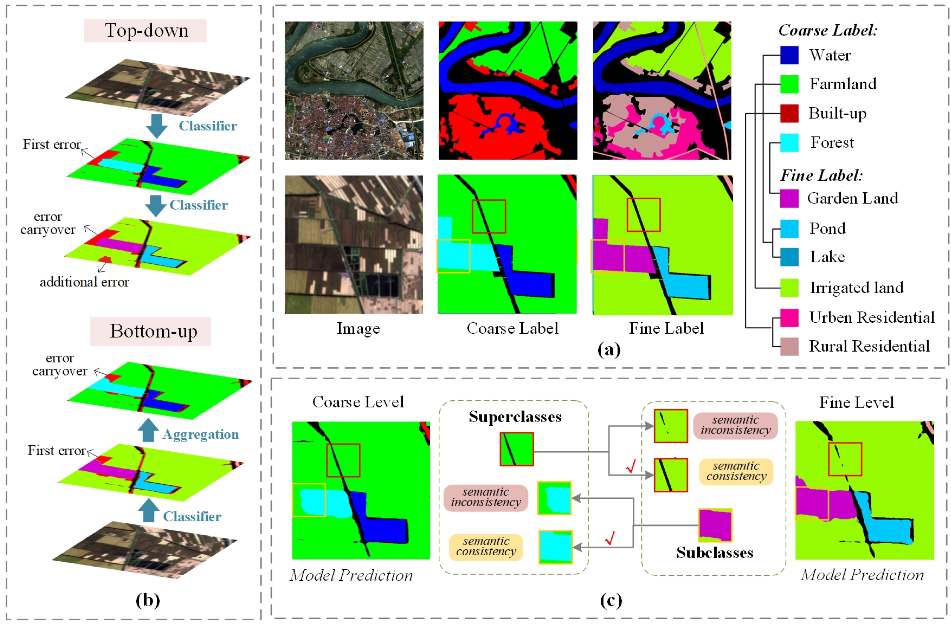
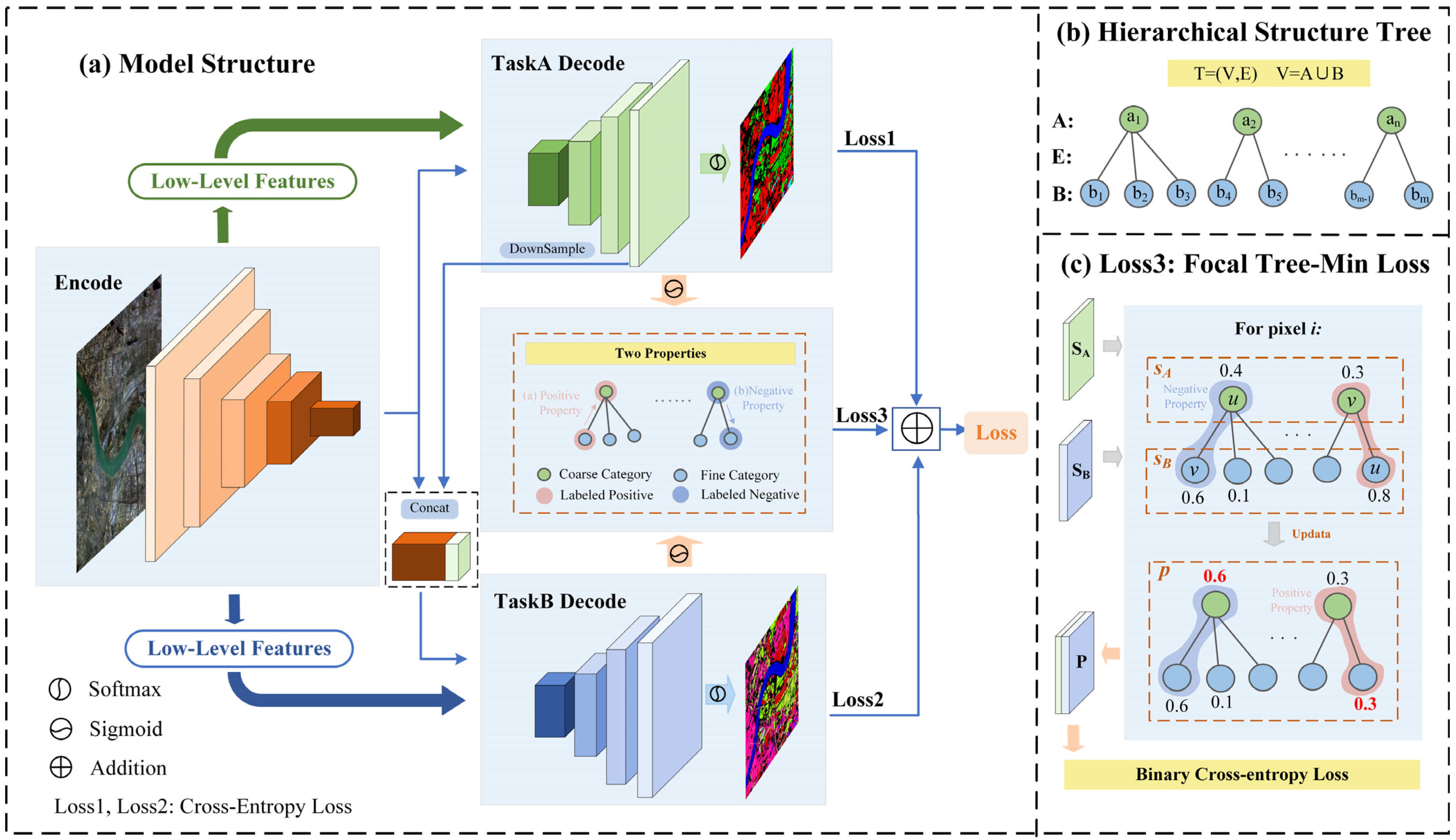
It achieves information sharing and mutual constraints between semantic layers through shared encoder and feature cascade, while independent decoders generate their respective classification maps, effectively preventing the accumulation and propagation of prediction errors across layers.

(2)

A hierarchical structure is incorporated into the loss function to explicitly model category dependencies, where a hierarchical regularization term, combined with task-specific losses, penalizes inconsistent predictions across semantic levels, thereby enhancing semantic coherence while maintaining high classification accuracy.

(3)

Two novel evaluation metrics, Semantic Alignment Deviation (SAD) and Enhancing Semantic Alignment Deviation (ESAD), are introduced to quantify semantic consistency across hierarchical levels by measuring the alignment of predictions with the taxonomic structure, offering a comprehensive assessment of both accuracy and coherence.

2. Related Work

2.1. Classification with Hierarchical Class Structures

In computer vision, many scholars have studied the hierarchical image classification problem across multiple semantic levels, modeling different types of semantic relationships to improve classification accuracy. Some studies directly use explicit hierarchical structures in networks, such as hierarchical graph structures [28] and semantic neuron graph networks [29], to model hierarchical relationships, but they need to explore potential semantic relationships further. Deng et al. [30] introduced the Hierarchy and Exclusive (HEX) graph to construct semantic relationships, proposing a CNN that uses the HEX graph for training and inference, outputting class probabilities at each level and producing hierarchically consistent results. Building on this, Chen et al. [31] combined the probabilistic classification loss of the HEX graph with a hybrid loss function involving cross-entropy to address the hierarchical multi-label ship recognition problem in remote sensing images. Zhang et al. [32] also used hierarchical knowledge graphs to describe label correlations between scenes and objects. Jo et al. [33] proposed a hierarchical extraction algorithm based on Directed Acyclic Graphs (DAGs), calculating conditional probabilities between classes to estimate the class correlation matrix and generate hierarchies based on a threshold. These methods acquire semantic hierarchical relationships through modeling or derivation. However, the suggested training and inference procedure is complex and time-consuming.

To reduce reliance on the model, some researchers have optimized the loss function to capture semantic hierarchical relationships and defined hierarchical constraints based on the hierarchy [34,35]. Hierarchical constraints refer to the requirement that when a data point belongs to a subclass, it must also belong to all superclasses of that subclass. The Coherent Hierarchical Multi-Label Classification Networks (C-HMCNN) [35] incorporated hierarchical constraints into prediction and learning, modifying the standard binary cross-entropy loss function to teach the network how to effectively influence the prediction of higher-level categories when utilizing lower-level category predictions. Jo et al. [33] proposed a new loss function that utilizes hierarchical constraints, providing additional class relationship information to the classifier using the hierarchical structure. Furthermore, Li et al. [36] introduced another hierarchical constraint; if a data point does not belong to a parent class, all the subclasses under that parent class should be labeled as negative. By strengthening label dependencies and constraints in the tree structure, these methods further improve classification consistency and semantic expression during prediction and learning.

2.2. Multi-Level Land Cover Classification

Multi-level land cover classification follows a predefined scheme to generate multi-level classification maps. While some studies produced results at various levels, they did not explicitly consider hierarchical structure constraints during classification [37,38]. Sulla-Menashe et al. [37] perform independent classification at each level, generating posterior probabilities using a model and adjusting them with external auxiliary information to obtain final results. HierU-Net [38] uses a dual U-shaped network to simultaneously classify land cover at coarse and fine levels, with coarse-level outputs acting as soft constraints for fine-level segmentation. Many studies have incorporated hierarchical structures into land cover classification and adopted a top-down strategy. Gavish et al. [11] introduced a Hierarchical Random Forest (HRF) method, training local classifiers at each internal node to select categories sequentially along the tree structure. Demirkan et al. [12] and Waśniewski et al. [14] first conducted a preliminary classification using various spectral indices (e.g., NDWI and NDVI), which were then subdivided into multiple subclasses. Additionally, some studies have employed bottom-up strategies, first generating low-level classification results and then progressively aggregating them to construct higher-level classification maps [15,16]. The accuracy of these methods heavily relies on the quality of initial predictions, usually generated through machine learning, which limits accuracy. Moreover, errors in the initial predictions tend to propagate and amplify in later stages, making it increasingly difficult to rectify.

Deep learning methods have been proposed for hierarchical land cover classification to overcome these limitations. Yang et al. [13] proposed a CNN-based model, LuNet-MT, employing two prediction strategies—coarse-to-fine (C2F) and fine-to-coarse (F2C)—to maintain consistency with the object hierarchy. However, this method requires multiple iterations, which reduces computational efficiency. LuNet-lite-MT [39] addressed this issue by introducing a Joint Optimization (JO) approach that predicts by selecting hierarchical tuples with the maximum joint category scores across all levels, obtaining predictions for all levels simultaneously and reducing the need for multiple iterations. Additionally, Recurrent Neural Network (RNN) architectures have been employed. For instance, Gbodjo et al. [40] used a hierarchical pre-training strategy, training the network from the top level and transferring weights to lower levels. However, this method cannot simultaneously predict all classes within the hierarchy and overlooks inter-level dependencies. HCS-ConvRNN [10] improved upon this by facilitating information transfer among levels, enabling simultaneous classification at multiple semantic levels. These studies suggest that inter-level information sharing can substantially improve the accuracy and consistency of hierarchical land cover classification.

2.3. Deep Multi-Task Learning

Multi-task learning (MTL) is a learning paradigm in machine learning, and its aim is to leverage useful information contained in multiple related tasks to help improve the generalization performance of all the tasks [41]. Deep multi-task learning is the application of MTL in deep learning, utilizing deep neural networks to handle multiple tasks and improving performance through shared low-level features and end-to-end training. The architecture of deep multi-task learning is generally classified into the following two categories: hard parameter sharing [42,43,44] and soft parameter sharing [45,46,47]. Soft parameter sharing allocates independent parameter sets for each task, facilitating information exchange through feature sharing mechanisms. However, its parameter size and computational complexity grow linearly with the number of tasks, limiting scalability. In contrast, hard parameter sharing models share low-level features and branch the task output layers at designated points, thus avoiding redundant computations. UPerNet [42] is a hard parameter sharing model that simultaneously processes low-level, mid-level, and high-level visual tasks, branching at each stage’s feature maps to handle different semantic parsing tasks. PAD-Net [43] and MTI-Net [44] branches after the encoder to produce intermediate predictions, which are further refined by related tasks through a multi-modal distillation module. With the remarkable advantages of Transformer in capturing long-range dependencies and multi-scale feature representations, Transformer-based hard parameter sharing models exhibit superior performance in multi-task learning, especially in handling complex semantic associations and cross-task information sharing [48,49]. Despite performance improvements from these architectural designs, they need to explicitly incorporate semantic relationships into the network, which limits their ability to model a clear hierarchy of visual concepts. Therefore, a hierarchical structure is explicitly incorporated into the loss function to model semantic relationships between tasks, enabling the synchronized optimization of classification results across multiple levels.

3. Methodology

The framework follows an encoder–decoder structure, as shown in Figure 2. First, VHR images are fed into a shared encoder, allowing the model to capture and leverage potential hierarchical relationships within the data naturally. Second, task-specific decoders handle individual semantic segmentation tasks, while sharing information through feature cascades, facilitating the targeted learning of task-specific features. Finally, introducing a hierarchical loss function enhances the model’s understanding of hierarchical relationships, guiding it to focus on the category structure during training. This approach enables the model to automatically discover and learn hierarchical relationships and optimizes them through the loss mechanism, delivering an improved land cover classification performance.

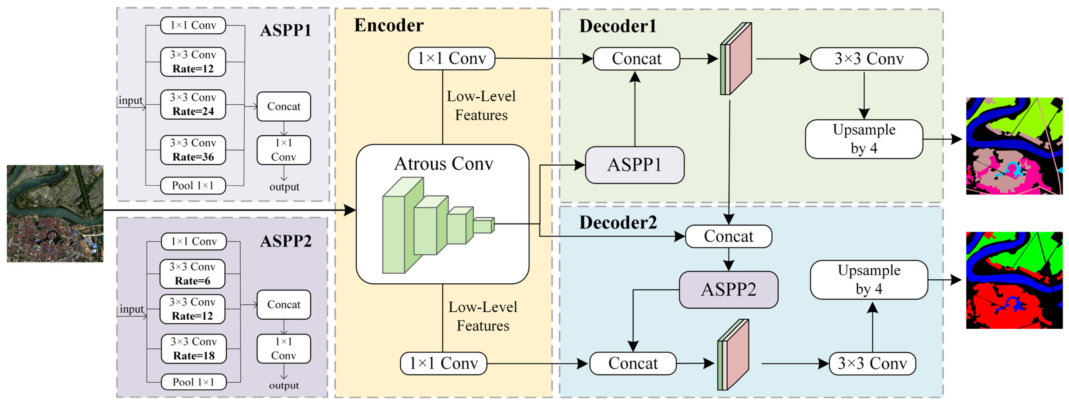
3.1. Encode–Decode Structure

The encoder serves as the network’s core module, extracting high-level feature representations from input data. Sharing irrelevant features between different tasks in the encoder lowers the efficiency of feature extraction. Premature branching may also result in insufficient sharing, diminishing the collaborative advantages between tasks. In this study, given the strong semantic correlation between coarse- and fine-level segmentation tasks, branching occurs after the entire encoder is shared, facilitating the more effective capture of low-level common features, promoting collaboration and facilitating information exchange between tasks. Compared to traditional single-task learning (STL), this shared mechanism reduces model complexity and enhances the potential for associative learning across tasks.

Each task maintains an independent decoder during the decoding phase to process features based on its specific classification requirements. To enhance interrelation and information sharing among tasks, we introduced a feature cascade strategy. The segmentation results from the first task are combined with the high-level features from the shared encoder to serve as the input for the next task, providing additional contextual information for subsequent tasks. Feature cascade ensures a smooth and consistent flow of information from initial coarse predictions to more refined outputs, facilitating complementarity and enhancement among different semantic layers. This design significantly improves the model’s overall performance in complex scenarios, ensuring semantic consistency across various tasks (coarse-level segmentation and fine-level segmentation tasks) and enhancing the prediction accuracy of multi-level segmentation tasks.

The DeepLabv3+ model adopts an encoder–decoder architecture, integrating depth-wise separable convolutions and atrous spatial pyramid pooling (ASPP), which enhances the capture of multi-scale contextual information while preserving spatial details. Using the DeepLabv3+ model as a foundation, we extend its architecture into a multi-task cascade framework (MTL-SCH) (Figure 3). The detailed steps are as follows:

(1)

Encoder component

The encoder employs a ResNet50 backbone with atrous convolutions to extract hierarchical features from the input VHR image. Specifically, low-level features, which contain rich spatial and structural information, are extracted from earlier layers and passed through 1 × 1 convolutions to reduce the channel dimension. These are later used in the decoding phase to aid spatial detail recovery. High-level features, which carry semantic context, are captured via atrous convolutions with increasing dilation rates. These features serve as shared inputs to multiple decoders, enabling joint learning across semantic levels.

(2)

Decoder1: Coarse-level segmentation

The shared high-level features are fed into the first Atrous Spatial Pyramid Pooling module (ASPP1) with dilation rates [12,24,36], which are designed to capture broad contextual information. The ASPP1 output is concatenated with the low-level features (after 1 × 1 conv) to combine semantic and spatial information. This fused feature map is then passed through a 3 × 3 convolutional layer and upsampled by a factor of 4 to generate the coarse-level segmentation result. Decoder1 is optimized to focus on coarse classification targets, such as broader land cover categories.

(3)

Decoder2: Fine-level segmentation

Parallel to Decoder1, Decoder2 also takes the shared high-level features as input. It uses another ASPP module (ASPP2) with dilation rates [6,12,18]. This allows the decoder to focus on more localized and detailed semantics. To enhance semantic consistency between hierarchical levels, Decoder2 also integrates the output features from Decoder1 via channel-wise concatenation. The concatenated features are passed through additional convolutional and upsampling layers to produce the fine-level segmentation result. Decoder2 thus benefits from both shared encoder features and semantic cues from Decoder1, achieving better spatial precision and hierarchical consistency.

(4)

Feature cascade

To promote semantic consistency across hierarchical levels, this study employs a direct concatenation strategy to merge features between decoders. Specifically, the feature map from Decoder1 is concatenated with the shared high-level features received by Decoder2 along the channel dimension, forming an enhanced composite representation. This combined feature map is then passed into ASPP2 for further processing, enabling Decoder2 to effectively integrate both coarse-level semantic priors and fine-grained contextual features. By leveraging the semantic hierarchy established by Decoder1, Decoder2 can achieve a more precise and semantically aligned prediction at the fine level. This approach facilitates stronger task synergy, enhances cross-level semantic consistency, and ultimately improves the overall segmentation performance of the network.

During training, each decoder is supervised by task-specific objectives. By simultaneously optimizing both decoders, the network learns to balance shared representations and task-specific refinements. The concatenation operation between Decoder1 and Decoder2 facilitates cross-task feature sharing, enabling the better integration of coarse-to-fine semantics.

3.2. Hierarchical Loss Functions

3.2.1. Focal Tree-Min Loss

To ensure the hierarchical consistency in land cover classification, a new loss function has been proposed to account for class hierarchy [39]. This loss function maximizes the joint class scores for correct tuples and minimizes them for incorrect tuples. While this approach ensures the consistency of classification results within the hierarchical structure, it may reduce the accuracy of the classification results. Therefore, we introduce the Focal Tree-Min Loss functions [36]. Focal Tree-Min Loss (${\mathrm{L}}_{\mathrm{F}\mathrm{T}\mathrm{M}}$) is a hierarchy-based loss function that treats the semantic segmentation task as a pixel-wise multi-label classification task. A hierarchically consistent score map $\mathrm{P}$, which strictly adheres to hierarchical constraints, is constructed. Due to its design, any violation of the hierarchical structure is explicitly penalized rather than merely penalizing individual misclassifications.

In this study, all semantic classes are formalized into a hierarchical tree structure $\mathrm{T}=(\mathrm{V},\mathrm{E})$, as shown in Figure 2b. Here, $\mathrm{A}=\{{\mathrm{a}}_1,{\mathrm{a}}_2,\dots ,{\mathrm{a}}_{\mathrm{n}}\}$ is the label set for the coarse-level task, $\mathrm{B}=\left\{{\mathrm{b}}_1,{\mathrm{b}}_2,\dots ,{\mathrm{b}}_{\mathrm{m}}\right\}$ is the label set for the fine-level task, $\mathrm{V}=\mathrm{A}\cup \mathrm{B}$ represents the set of all nodes, and the edge set $\mathrm{E}$ represents the relationships between superclasses and subclasses. For example, if ${\mathrm{b}}_1,{\mathrm{b}}_2,{\mathrm{b}}_3$ are subclasses of ${\mathrm{a}}_1$, then the edges ${(\mathrm{a}}_1,{\mathrm{b}}_1),{(\mathrm{a}}_1,{\mathrm{b}}_2),{(\mathrm{a}}_1,{\mathrm{b}}_3)\in \mathrm{E}$. This function needs to adhere to two fundamental properties to achieve hierarchical consistency.

(1)

Positive Property: For each pixel, if a class is labeled positive, all its ancestor nodes (i.e., superclasses) should be labeled positive.

(2)

Negative Property: For each pixel, if a class is labeled negative, all its child nodes (i.e., subclasses) should be labeled negative.

Based on these two properties, ${\mathrm{L}}_{\mathrm{F}\mathrm{T}\mathrm{M}}$ recalculates the prediction scores for each pixel by establishing positive $\mathrm{T}$-constraints and negative $\mathrm{T}$-constraints. It ensures that all predictions of category labels in pixel-level predictions satisfy hierarchical constraints. The two constraints are as follows:

(1)

Positive $\mathrm{T}$-Constraint: For each pixel $\mathrm{i}$, if class $\mathrm{v}\in \mathrm{V}$ is labeled as positive (belongs to this class), and $\mathrm{u}\in {\mathrm{V}}_{\mathrm{A}}$, then it should hold that ${\mathrm{S}}_{\mathrm{v}}\le {\mathrm{S}}_{\mathrm{u}}$.

(2)

Negative $\mathrm{T}$-Constraint: For each pixel $\mathrm{i}$, if class $\mathrm{v}\in \mathrm{V}$ is labeled as negative (does not belong to this class), and $\mathrm{u}\in {\mathrm{V}}_{\mathrm{B}}$, then it should hold that ${1-\mathrm{S}}_{\mathrm{v}}\le {1-\mathrm{S}}_{\mathrm{u}}$.

Where, V denotes all node sets, $\mathrm{v}\in$ V represents a node, ${\mathrm{S}}_{\mathrm{v}}$ represents the probability score of node v, and ${\mathrm{S}}_{\mathrm{u}}$ represents the probability score of node u, which is associated with v. Here, u is an index variable whose role depends on the category of v, as follows: when v ∈ ${\mathrm{V}}_{\mathrm{A}}$ (the coarse-level node set), u ∈ ${\mathrm{V}}_{\mathrm{B}}$ (the fine-level node set); when v ∈ ${\mathrm{V}}_{\mathrm{B}}$, u ∈ ${\mathrm{V}}_{\mathrm{A}}$; when v is a positive class, the probability score ${\mathrm{S}}_{\mathrm{u}}$ of the associated node u should exceed or be equal to the probability score ${\mathrm{S}}_{\mathrm{v}}$ of node v; and when v is a negative class, the probability score ${\mathrm{S}}_{\mathrm{u}}$ of the associated node u should not exceed the probability score ${\mathrm{S}}_{\mathrm{v}}$ of node v.

The segmentation network outputs two score maps, one is the coarse-level score map ${\mathrm{S}}_{\mathrm{A}}=\mathrm{s}\mathrm{i}\mathrm{g}\mathrm{m}\mathrm{i}\mathrm{o}\mathrm{d}\left({\mathrm{f}}_{\mathrm{S}\mathrm{E}\mathrm{G}1}\left(\mathrm{I}\right)\right)\in {[0,1]}^{\mathrm{H}\times \mathrm{W}\times \mathrm{n}}$, and the other is the fine-level score map ${\mathrm{S}}_{\mathrm{B}}=\mathrm{s}\mathrm{i}\mathrm{g}\mathrm{m}\mathrm{i}\mathrm{o}\mathrm{d}\left({\mathrm{f}}_{\mathrm{S}\mathrm{E}\mathrm{G}2}\left(\mathrm{I}\right)\right)\in {[0,1]}^{\mathrm{H}\times \mathrm{W}\times \mathrm{m}}$. To ensure the satisfaction of the two hierarchical constraints mentioned above, a hierarchically consistent score map $\mathrm{P}$ is calculated from ${\mathrm{S}}_{\mathrm{A}}$ and ${\mathrm{S}}_{\mathrm{B}}$. For each pixel $\mathrm{i}$, the updated score vector $p={\left[p_v\right]}_{\mathrm{v}\in \mathrm{V}}\in {\left[0,1\right]}^{\left|\mathrm{V}\right|}$ is computed as follows:

$$\left\{\begin{array}{cc}{p}_v=\underset{\mathrm{u}\in {\mathrm{V}}_{\mathrm{A}}}{\min }\left(s_{A\left(u\right)}\right)& \mathrm{if}{\widehat{\mathrm{l}}}_{\mathrm{v}}=1,\hfill \\ 1-p_v=\underset{\mathrm{u}\in {\mathrm{V}}_{\mathrm{B}}}{\min }\left(1-s_{B\left(u\right)}\right)=1-\underset{\mathrm{u}\in {\mathrm{V}}_{\mathrm{B}}}{\max }\left(s_{B\left(u\right)}\right)& \mathrm{i}\mathrm{f}{\widehat{\mathrm{l}}}_{\mathrm{v}}=0,\hfill \end{array}\right.$$

(1)

where $s_A={\left[s_{A\left(u\right)}\right]}_{\mathrm{u}\in {\mathrm{V}}_{\mathrm{A}}}\in {\mathrm{S}}_{\mathrm{A}},s_B={\left[s_{B\left(u\right)}\right]}_{\mathrm{u}\in {\mathrm{V}}_{\mathrm{B}}}\in {\mathrm{S}}_{\mathrm{B}}$ refers to the original score vector of pixel $\mathrm{i}$. With Equation (1), the pixel-wise prediction $\mathrm{P}$ is guaranteed to always satisfy the hierarchy constraints. Notably, each class is both a subclass and a superclass of itself. When ${\widehat{\mathrm{l}}}_{\mathrm{v}}=1$, it indicates that the node $\mathrm{v}\in \mathrm{V}$ is a positive class, and its scope ${\mathrm{p}}_{\mathrm{v}}$ is the minimum score of all ancestor nodes ${\mathrm{s}}_{\mathrm{A}\left(\mathrm{u}\right)}$, which ensures that the positive $\mathrm{T}$-constraint is satisfied. When ${\widehat{\mathrm{l}}}_{\mathrm{v}}=0$, it indicates that the node $\mathrm{v}\in \mathrm{V}$ is a negative class, and the opposite of its score $1-{\mathrm{p}}_{\mathrm{v}}$ is the minimum of the opposite scores of all child nodes (i.e., the maximum of the original scores), which ensures that the negative $\mathrm{T}$-constraint is satisfied. Treat the updated score map $\mathrm{P}$ as the probability result obtained from multi-label classification. Calculate the binary cross-entropy for each category $\mathrm{v}$ (i.e., ${\mathrm{p}}_{\mathrm{v}}$), sum over all categories, and substitute Equation (1) into it. The specific formula is as follows:

$$\begin{gathered} {\mathrm{L}}_{\mathrm{T}\mathrm{M}}=\sum _{\mathrm{v}\in \mathrm{V}}-{\widehat{\mathrm{l}}}_{\mathrm{v}}\log \left(p_v\right)-\left(1-{\widehat{\mathrm{l}}}_{\mathrm{v}}\right)\log \left(1-p_v\right) \\ {\displaystyle \hspace{1em}\hspace{1em}\hspace{1em}\hspace{1em}={\sum }_{\mathrm{v}\in \mathrm{V}}-{\widehat{\mathrm{l}}}_{\mathrm{v}}\log \left(\underset{\mathrm{u}\in {\mathrm{V}}_{\mathrm{A}}}{\min }\left(s_{A\left(u\right)}\right)\right)- \\ \hspace{1em}\hspace{1em}\hspace{1em}\hspace{1em}\left(1-{\widehat{\mathrm{l}}}_{\mathrm{v}}\right)\log \left(1-\underset{\mathrm{u}\in {\mathrm{V}}_{\mathrm{B}}}{\max }\left(s_{B\left(u\right)}\right)\right)} \end{gathered}$$

(2)

A modulation factor has been added to the Tree-Min Loss to reduce the relative loss on well-classified pixel samples and to focus attention on those difficult pixel samples. According to the above constraints, the ${\mathrm{L}}_{\mathrm{F}\mathrm{T}\mathrm{M}}$ is defined as follows:

$$\begin{gathered} {\mathrm{L}}_{\mathrm{F}\mathrm{T}\mathrm{M}}={\sum }_{\mathrm{v}\in \mathrm{V}}-{\widehat{\mathrm{l}}}_{\mathrm{v}}{\left(1-p_v\right)}^{\mathsf{\gamma }}\log \left(p_v\right)-\left(1-{\widehat{\mathrm{l}}}_{\mathrm{v}}\right)p_v^{\gamma }\log \left(1-p_v\right) \\ {\displaystyle \hspace{1em}\hspace{1em}\hspace{1em}={\sum }_{\mathrm{v}\in \mathrm{V}}-{\widehat{\mathrm{l}}}_{\mathrm{v}}{\left(1-\underset{\mathrm{u}\in {\mathrm{V}}_{\mathrm{A}}}{\min }\left(s_{A\left(u\right)}\right)\right)}^{\mathsf{\gamma }}\log \left(\underset{\mathrm{u}\in {\mathrm{V}}_{\mathrm{A}}}{\min }\left(s_{A\left(u\right)}\right)\right)- \\ \hspace{1em}\hspace{1em}\hspace{1em}\left(1-{\widehat{\mathrm{l}}}_{\mathrm{v}}\right){\left(\underset{\mathrm{u}\in {\mathrm{V}}_{\mathrm{B}}}{\max }\left(s_{B\left(u\right)}\right)\right)}^{\mathsf{\gamma }}\log \left(1-\underset{\mathrm{u}\in {\mathrm{V}}_{\mathrm{B}}}{\max }\left(s_{B\left(u\right)}\right)\right)} \end{gathered}$$

(3)

where $\mathsf{\gamma }\ge 0$ is a tunable focal parameter used to control the degree to which easy samples are downweighted. When $\mathsf{\gamma }=0$, ${\mathrm{L}}_{\mathrm{F}\mathrm{T}\mathrm{M}}$ is equivalent to ${\mathrm{L}}_{\mathrm{T}\mathrm{M}}$.

3.2.2. Joint Loss Function

In the multi-task learning framework, the total loss function is optimized by adding the losses of two tasks [42]. However, due to the consistency requirement in the hierarchical structure, relying solely on the cross-entropy loss may not ensure hierarchical consistency in classification. Therefore, we introduce ${\mathrm{L}}_{\mathrm{F}\mathrm{T}\mathrm{M}}$ on top of the losses of the two tasks, encouraging the network to achieve good classification performance on each task, while guiding the prediction results between tasks to maintain consistency in the hierarchical structure, thus improving the network’s overall generalization ability and the model’s interpretability. The modified joint loss function is as follows:

$$\mathrm{L}={\mathrm{L}}_{\mathrm{A}}+{\mathrm{L}}_{\mathrm{B}}+{\mathrm{L}}_{\mathrm{F}\mathrm{T}\mathrm{M}}$$

(4)

where ${\mathrm{L}}_{\mathrm{A}}$ and ${\mathrm{L}}_{\mathrm{B}}$ is the classification loss for a specific task, typically cross-entropy loss. ${\mathrm{L}}_{\mathrm{F}\mathrm{T}\mathrm{M}}$ is focal tree-min loss, used to ensure that the prediction results between coarse and fine-level segmentation tasks conform to the hierarchical structure.

4. Experiments and Results

In this section, we first conducted ablation experiments based on DeepLabV3+-SCH, systematically evaluating the contribution of each method to overall performance. We then compare Deeplabv3+-SCH with other related segmentation methods. Subsequently, we extended the MTL-SCH method to other network architectures, including SegFormer [50], UNetFormer [51], MANet [19], CMTFNet [52], SUNet [53], and SFFNet [54] to validate its generality and effectiveness. Furthermore, we analyzed the semantic segmentation consistency between coarse- and fine-level segmentation results across different networks to evaluate the performance of each model in capturing multi-level semantic information. Finally, the performance of MTL-SCH was further validated on the STB dataset.

4.1. Experimental Setup

4.1.1. Dataset

The GID dataset [22] is divided into the coarse-grained classification set (GID-5) and the fine-grained land cover set (GID-15), each suitable for different application scenarios and analytical purposes. The GID dataset is classified into a two-layer classification system based on semantic hierarchy, with detailed information on specific categories provided in

Table 1. Two levels of semantic classes for the GID dataset used in our experiments.

6-Class	16-Class
Background	Background (BB)
Built-Up	Industrial Land (IL), Urban Residential (UR), Rural Residential (RR), Traffic Land (TL)
Forest	Garden Land (GL), Arbor Forest (AF), Shrub Land (SL)
Farmland	Paddy Field (PF), Irrigated Land (IR), Dry Cropland (DC)
Meadow	Natural Meadow (NM), Artificial Meadow (AM)
Water	River (WR), Lake (WL), Pond (WP)

. This study utilized 10 remote sensing images with a size of 6800 × 7200 pixels, which were expanded into 8000 images with a resolution of 512 × 512 through sliding segmentation and data augmentation techniques, including rotation, flipping, Gaussian blur, color enhancement, and noise addition. These images were then randomly divided into a training set (80%) and a test set (20%).

The STB dataset is the remote sensing image segmentation dataset from the AI competition hosted by Huawei in 2020. The data includes high-resolution images from Gaofen-1, Gaofen-2, Gaofen-6, High-Resolution Satellite-2, Beijing-2, and some aerial sources, with resolutions ranging from 0.1 to 4 m, consisting of visible and multispectral payload images, all with a size of 256 × 256 pixels. The classification system for land cover features includes eight primary categories and 17 secondary subclasses, with specific classification details shown in

Table 2. Two levels of semantic classes for the STB dataset used in our experiments.

8-Class	17-Class
Water	Water (WW)
Transportation	Road (TR), Airport (TA), Railway Station (TS)
Impervious Surface (ISA)	Building (IB), Parking Lot (IL), Photovoltaic (IP), Playground (IG)
Agriculture	Cultivated Land (AC), Agriculture Greenhouse (AG)
Grass	Natural Grass (GN), Unnatural Grass (GU)
Forest	Natural Forest (FN), Unnatural Forest (FU)
Barren	Natural Bare Soil (BN), Unnatural Bare Soil (BU)
Other	Other (OO)

. The experiment selects 30,000 images from the dataset, and the training set will consist of 80% of the images, while the testing set will include the remaining 20%.

4.1.2. Parameter Settings

During the model training process, for CNN-based models, we used SGD as the optimizer with base learning rate 1 × 10⁻³, momentum 0.9, and weight decay 1 × 10⁻⁴. For Transformer-based models, we used Adam as the optimizer with the base learning rate as 1 × 10⁻⁴ and weight decay as 0.01. All backbones are initialized using the weights pre-trained on ImageNet-1K, while the remaining layers are randomly initialized. The MTL-SCH framework (e.g., DeepLabv3+-SCH) and the STL method (e.g., DeepLabv3+) adopt the same parameter settings to ensure a fair comparison of their effectiveness, and all models have converged. We set the batch size to 16 for both the GID and the STB datasets and trained for 50 epochs. Both the training and testing processes were implemented using the PyTorch framework (version 2.6.0), and the model was trained on an NVIDIA RTXA6000 with 48 GB GPU memory (NVIDIA Corporation, Santa Clara, CA, USA).

In the Focal Tree-Min Loss, the modulation factor γ plays a critical role in controlling the focus on hard versus easy samples. To investigate its influence on model performance, we conducted a sensitivity analysis by varying γ ∈ {0, 1, 2, 3} and evaluating the segmentation accuracy on the GID dataset using the DeepLabv3+-SCH backbone. The experimental results are summarized in

Table 3. Classification accuracy under different values of the modulation factor γ, where the bolded row indicates the experiment with the highest accuracy.

	Coarse Level			Fine Level
	OA	MIoU	FWIoU	OA	MIoU	FWIoU
γ = 0	90.24	82.37	82.35	88.46	75.80	79.49
γ = 1	90.12	82.33	82.21	88.44	76.52	79.52
γ = 2	90.09	82.27	82.12	88.34	75.92	79.37
γ = 3	89.88	82.00	81.75	88.17	75.93	79.02

.

It can be observed that the model achieves the highest performance when γ = 1, with the best mIoU and FWIoU scores at fine levels. This suggests that γ = 1 strikes a good balance between model stability and the selective emphasis on misclassified or low-confidence samples. When γ is set to 0, the loss degenerates into a standard Tree-Min Loss, leading to slightly lower fine-level accuracy. On the other hand, larger γ values (e.g., γ = 2 or 3) tend to overly penalize difficult samples, which may reduce overall performance by neglecting well-learned structures. Based on these results, we select γ = 1 as the default setting in our experiments.

4.2. Evaluation Metrics

4.2.1. Segmentation Accuracy Metrics

The model’s performance is evaluated by calculating the overall accuracy (OA), mean intersection over union (mIoU), and frequency-weighted intersection over union (FWIoU) between the model predictions and the ground truth. These metrics are used to evaluate the accuracy and performance of the model in segmentation tasks, focusing primarily on the overall performance of the model across all categories. IoU measures the overlap between predicted and ground truth regions. MIoU calculates the average IoU across all classes, providing insights into the model’s ability to accurately segment multiple classes simultaneously. FWIoU takes into account both per-class IoU and class frequency [55]. The specific definitions are as follows:

$$\mathrm{O}\mathrm{A}=\frac{{\sum }_{\mathrm{i}=1}^{\mathrm{k}}{\mathrm{P}}_{\mathrm{i}\mathrm{i}}}{{\sum }_{\mathrm{i}=1}^{\mathrm{k}}{\sum }_{\mathrm{j}=1}^{\mathrm{k}}{\mathrm{P}}_{\mathrm{i}\mathrm{j}}}$$

(5)

$$\mathrm{m}\mathrm{I}\mathrm{o}\mathrm{U}={\displaystyle \frac{1}{\mathrm{k}+1}}{\sum }_{\mathrm{i}=1}^{\mathrm{k}}{\displaystyle \frac{{\mathrm{P}}_{\mathrm{i}\mathrm{i}}}{{\sum }_{\mathrm{j}=1}^{\mathrm{k}}{\mathrm{P}}_{\mathrm{i}\mathrm{j}}+{\sum }_{\mathrm{j}=1}^{\mathrm{k}}{\mathrm{P}}_{\mathrm{j}\mathrm{i}}-{\mathrm{P}}_{\mathrm{i}\mathrm{i}}}}$$

(6)

$$\mathrm{F}\mathrm{W}\mathrm{I}\mathrm{o}\mathrm{U}={\displaystyle \frac{1}{{\sum }_{\mathrm{i}=1}^{\mathrm{k}}{\sum }_{\mathrm{j}=1}^{\mathrm{k}}{\mathrm{P}}_{\mathrm{i}\mathrm{j}}}}{\sum }_{\mathrm{i}=0}^{\mathrm{k}}{\displaystyle \frac{{\sum }_{\mathrm{j}=1}^{\mathrm{k}}{\mathrm{P}}_{\mathrm{i}\mathrm{j}}{\mathrm{P}}_{\mathrm{i}\mathrm{i}}}{{\sum }_{\mathrm{j}=1}^{\mathrm{k}}{\mathrm{P}}_{\mathrm{i}\mathrm{j}}+{\sum }_{\mathrm{j}=1}^{\mathrm{k}}{\mathrm{P}}_{\mathrm{j}\mathrm{i}}-{\mathrm{P}}_{\mathrm{i}\mathrm{i}}}}$$

(7)

where ${\mathrm{p}}_{\mathrm{i}\mathrm{i}}$, ${\mathrm{p}}_{\mathrm{i}\mathrm{j}}$, ${\mathrm{p}}_{\mathrm{j}\mathrm{i}}$ represent the number of true positives, false positives, and false negatives, respectively. $\mathrm{k}$ is the number of classes.

4.2.2. Semantic Consistency Metrics

To quantitatively evaluate the effectiveness of this method in eliminating semantic ambiguity, we propose two new evaluation metrics—Semantic Alignment Deviation (SAD) and Enhancing Semantic Alignment Deviation (ESAD)—which assess the degree of consistency between different semantic levels in the model. Specifically, the lower the SAD and ESAD values, the smaller the semantic deviation, indicating reduced ambiguity between semantics. This means the model performs better in capturing and maintaining semantic consistency across different levels.

The SAD metric quantifies the inconsistency between semantic levels by calculating the proportion of areas where coarse- and fine-level labels are inconsistent in the segmentation results. For example, in areas labeled as forest at the coarse level, a certain proportion of pixels may be labeled as water or farmland at the fine level, which are not subclasses of forest. Thus, these areas exhibit semantic ambiguity, and this metric reflects the degree of conflict in segmentation results across different semantic levels. The ESAD combines semantic consistency with classification accuracy, further capturing cases where coarse- and fine-level segmentation results may be consistent, yet the classification results still need to be corrected. The ESAD can provide a more comprehensive reflection of the model’s overall performance.

$$\mathrm{S}\mathrm{A}\mathrm{D}=\frac{\sum _{\mathrm{i}=1}^{\mathrm{N}}\sum _{\mathrm{j}=1}^{\mathrm{M}}\mathbb{I}\left({\mathrm{C}}_{\mathrm{H}}\left(\mathrm{i}\right)\ne {\mathrm{C}}_{\mathrm{L}}\left(\mathrm{j}\right)\right)\cdot \mathrm{A}\left(\mathrm{i},\mathrm{j}\right)}{\mathrm{P}}$$

(8)

$$\mathrm{E}\mathrm{S}\mathrm{A}\mathrm{D}={\displaystyle \frac{\sum _{\mathrm{i}=1}^{\mathrm{N}}\sum _{\mathrm{j}=1}^{\mathrm{M}}\mathbb{I}\left({\mathrm{C}}_{\mathrm{H}}\left(\mathrm{i}\right)\ne {\mathrm{C}}_{\mathrm{L}}\left(\mathrm{j}\right)\left|\mathrm{o}\mathrm{r}\right|\mathrm{C}\left(\mathrm{i},\mathrm{j}\right)\ne \mathrm{T}\left(\mathrm{i},\mathrm{j}\right)\right)\cdot \mathrm{A}\left(\mathrm{i},\mathrm{j}\right)}{\mathrm{P}}}$$

(9)

where ${\mathrm{C}}_{\mathrm{H}}\left(\mathrm{i}\right)$ represents the $\mathrm{i}$-th region label at a high semantic level, ${\mathrm{C}}_{\mathrm{L}}\left(\mathrm{j}\right)$ represents the $\mathrm{j}$-th region label at a low semantic level, and $\mathbb{I}\left(\cdot \right)$ is the indicator function, which takes the value of 1 when the semantic level labels are inconsistent. $\mathrm{A}\left(\mathrm{i},\mathrm{j}\right)$ represents the overlapping pixels between the $\mathrm{i}$-th region at the high semantic level and the $\mathrm{j}$-th region at the low semantic level. ${\mathrm{C}}_{\mathrm{H}}\left(\mathrm{i}\right)\ne {\mathrm{C}}_{\mathrm{L}}\left(\mathrm{j}\right)$ indicates that the high-level label ${\mathrm{C}}_{\mathrm{H}}\left(\mathrm{i}\right)$ and the low-level label ${\mathrm{C}}_{\mathrm{L}}\left(\mathrm{j}\right)$ are inconsistent. $\mathrm{C}\left(\mathrm{i},\mathrm{j}\right)\ne \mathrm{T}\left(\mathrm{i},\mathrm{j}\right)$ indicates that the predicted label set $\mathrm{C}\left(\mathrm{i},\mathrm{j}\right)$ is inconsistent with the ground truth label set $\mathrm{T}\left(\mathrm{i},\mathrm{j}\right)$, where P is the total number of pixels.

4.3. Ablation Experiment

An ablation experiment is conducted to investigate the effectiveness of components in the proposed DeepLabv3+-SCH, including Share Features, Cascade Features, and Hierarchical Loss. The baseline represents a model comprising DeepLabv3+ with ResNet-50 as the backbone. This baseline network obtains segmentation results for both semantic layers at the coarse and fine levels. The experimental results of the test dataset are presented in the

Table 4. GID datasets ablation experiment on DeepLabv3+-SCH. The row in bold represents the experiment achieving the best accuracy. √ indicates that the component is selected.

Baseline	Share Feature	Cascade	Hierarchical Loss	Coarse Level			Fine Level
				OA	MIoU	FWIoU	OA	MIoU	FWIoU
√				88.66	80.14	79.83	86.25	72.8	76.13
√	√			89.46	81.26	81.11	87.6	74.5	78.17
√	√	√		89.59	81.66	81.26	87.84	75.22	78.48
√	√	√	√	90.12	82.33	82.21	88.44	76.52	79.52

.

On the GID dataset, when the single-task learning (STL) framework transitioned to using shared encoder features, the mIoU for the coarse level reached 81.26%, an improvement of 1.12% over the baseline. Simultaneously, the fine-level segmentation results are also improved, with the mIoU rising from 72.80% to 74.5%. Thus, shared encoder features contribute to the segmentation performance of both levels. After adding features, cascading on the shared encoder increased the fine-level mIoU from 74.5% to 75.22%, with minimal impact on coarse-level accuracy. This is because cascaded features fuse coarse-level and backbone features, primarily benefiting fine-level segmentation.

Furthermore, adding ${\mathrm{L}}_{\mathrm{F}\mathrm{T}\mathrm{M}}$ to the network, the fine-level mIoU and OA increased by 1.3% and 1.04%, while the coarse-level mIoU and OA increased by 0.67% and 0.53%. This indicates that the addition of ${\mathrm{L}}_{\mathrm{F}\mathrm{T}\mathrm{M}}$ improved the model’s performance. The optimal results are achieved when all components are implemented. Compared to the baseline, the mIoU values for both coarse and fine levels increased by 2.19% and 3.72%.

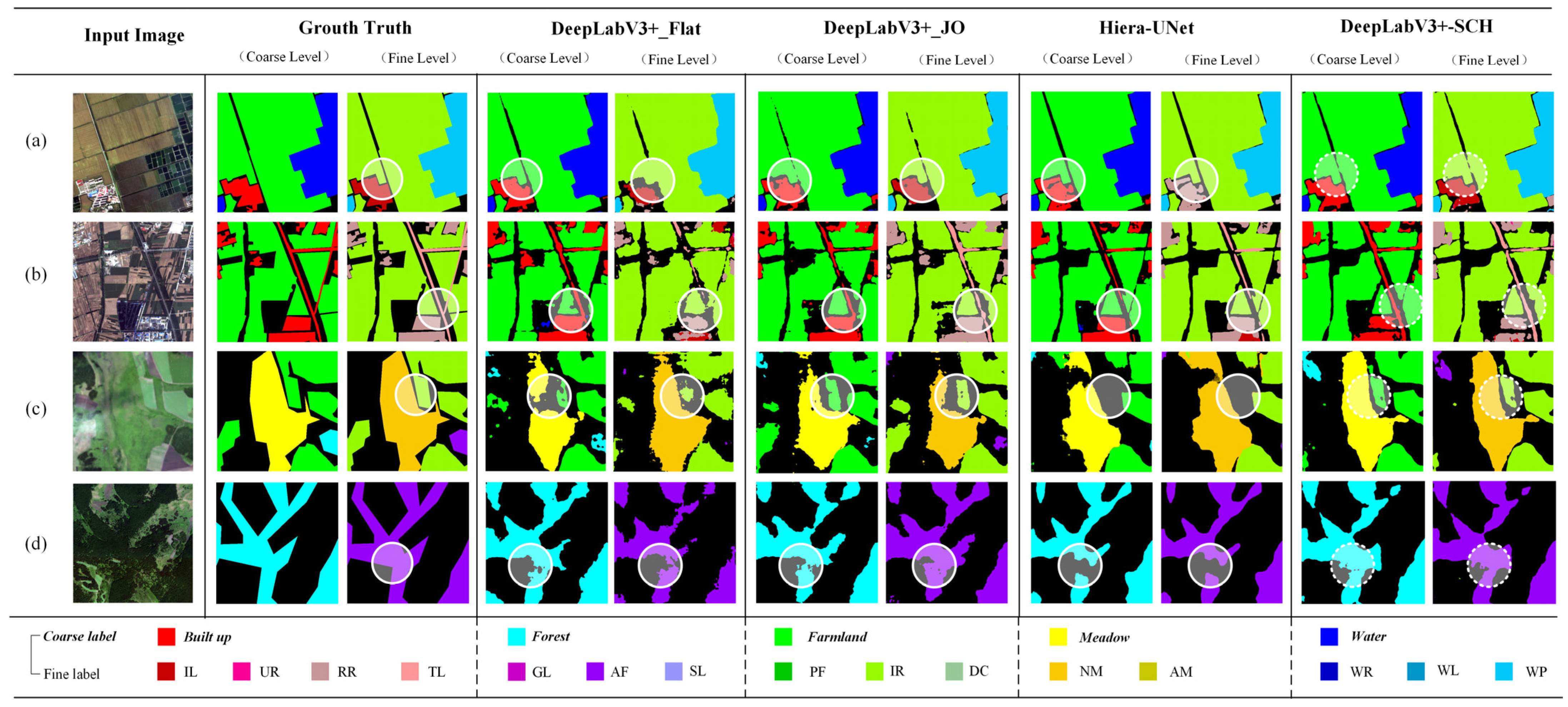
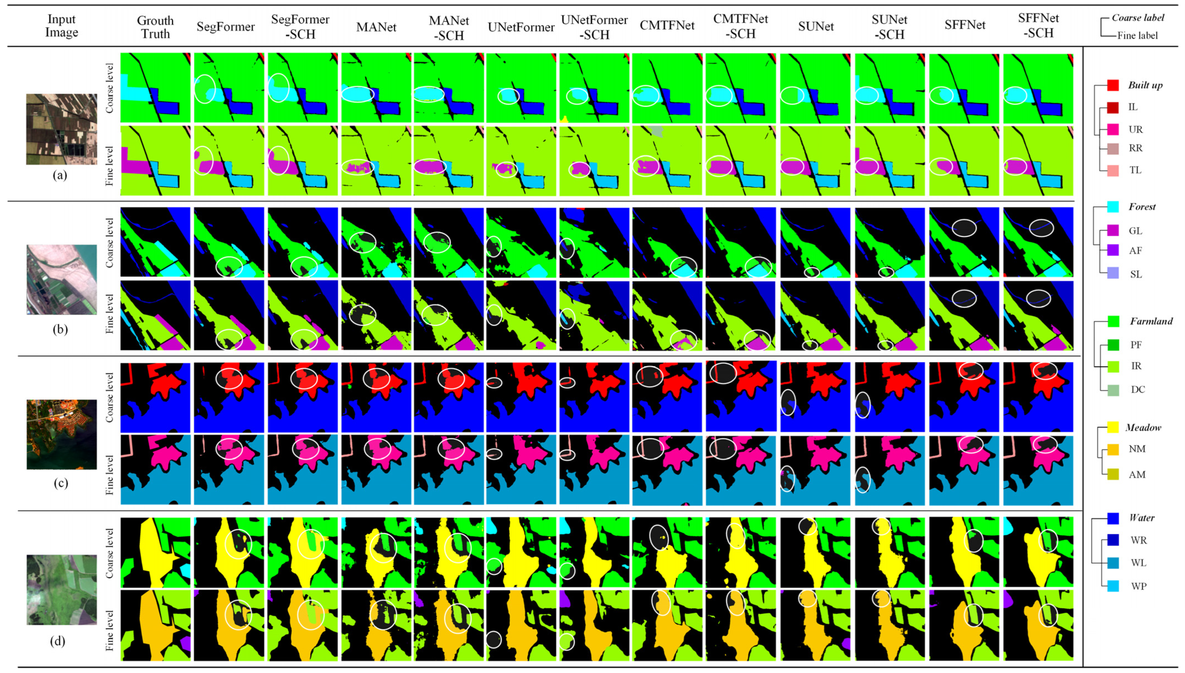
4.4. Experiments on the GID Dataset

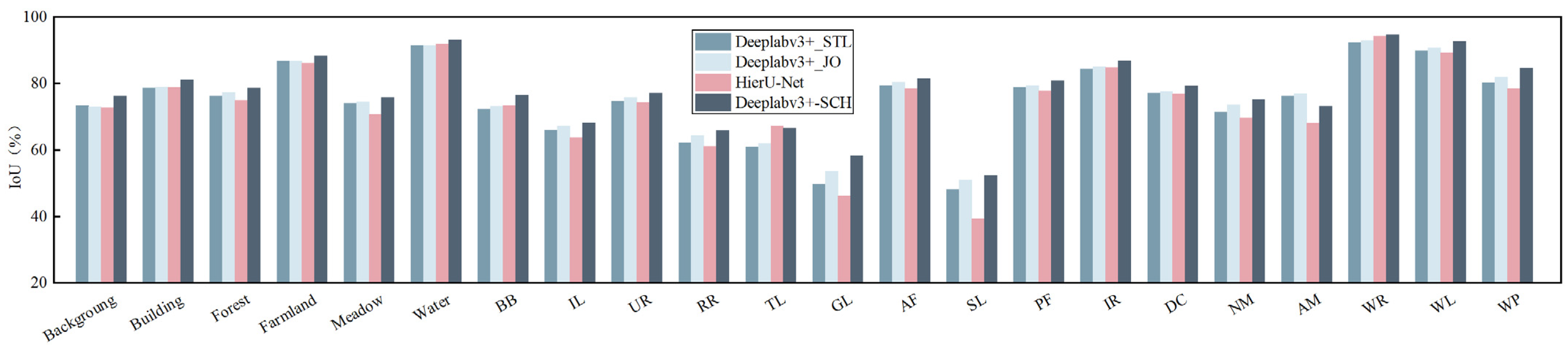
4.4.1. Comparative Experiments

To evaluate the effectiveness of the proposed MTL-SCH method, we compared it with other approaches for hierarchical land cover classification, including Single-Task Learning (STL), Joint Optimization (JO) [39], and HierU-Net [38]. STL performs land cover classification independently at a single semantic level without considering hierarchical relationships or multi-level semantic dependencies between classes. The Joint Optimization (JO) strategy introduces a novel loss function that incorporates the hierarchical structure of class labels during training. Classification is achieved by selecting hierarchical tuples with the highest joint class scores across all semantic levels. HierU-Net employs a dual U-shaped network architecture to classify coarse- and fine-level land cover. The coarse-level outputs are used as soft constraints, serving as input to the fine-level segmentation function to enhance performance.

In

Table 5. Performance comparison of different methods in terms of segmentation accuracies on GID datasets. The row in bold represents the experiment achieving the best accuracy.

FPS	Params (M)	Method	Backbone	Coarse Level			Fine Level			SAD	ESAD
				OA	MIoU	FWIoU	OA	MIoU	FWIoU
13.60	39.64	Deeplabv3+_STL	ResNet50	88.66	80.14	79.83	86.25	72.80	76.13	12.06	21.07
6.40	56.01	Deeplabv3+_JO	ResNet50	88.69	80.36	79.83	86.91	74.16	77.09	6.65	16.26
4.00	287.23	HierU-Net	ResNet50	88.37	79.27	79.34	86.45	71.51	76.45	1.96	14.55
7.38	56.06	Deeplabv3+-SCH	ResNet50	90.12	82.33	82.21	88.44	76.52	79.52	2.21	12.52

, we assess model complexity and inference efficiency using the number of parameters (Params) and frames per second (FPS). Higher Params indicate greater complexity and resource demands, while higher FPS reflects faster inference and better runtime efficiency. As shown, HierU-Net has the highest Params (287.23 M) and lowest FPS (4.00), indicating high complexity and slow speed. DeepLabv3+-STL achieves the highest FPS (13.60) with fewer Params (39.64 M) but requires a separate inference for coarse and fine tasks. DeepLabv3+-SCH strikes a balance with moderate Params (56.06 M) and FPS (7.38), benefiting from a shared encoder and unified decoding, enabling a single forward pass for both coarse and fine predictions, thus enhancing overall efficiency and deployment practicality.

The quantitative results on the test set are summarized in Table 5, providing a comprehensive comparison of segmentation accuracy at both coarse and fine levels. Compared to the STL baseline, the Deeplabv3+_JO strategy shows notable improvements in fine-level segmentation, increasing the mIoU from 72.80% to 74.16%. However, the proposed Deeplabv3+-SCH method consistently achieves the best performance across all metrics. Specifically, it obtains the highest mIoU scores at both the coarse level (82.33%) and fine level (76.52%), representing relative gains of 2.19% and 1.76% over the JO method and 3.06% and 5.01% over HierU-Net, respectively. Moreover, SCH also achieves the highest OA and FWIoU scores at both levels, demonstrating its ability to improve segmentation quality, while preserving semantic consistency across hierarchical categories. These results suggest that the proposed SCH framework can effectively leverage hierarchical supervision to enhance both coarse and fine-level predictions, promoting a better understanding of multi-level semantic structures in land cover classification.

Figure 4 illustrates the IoU values for all categories at both the coarse and fine levels. It can be observed that Deeplabv3+-SCH achieves the best IoU performance in the majority of categories, indicating its strong capability in modeling diverse semantic classes. Notably, significant improvements are observed in classes such as road, river, urban residential, and industrial land, which typically involve complex spatial boundaries and inter-class ambiguity. Although the performance on the artificial meadow (AM) class is slightly lower than that of other methods, the overall advantage of SCH remains evident. These results collectively demonstrate that the proposed MTL-SCH framework effectively leverages hierarchical supervision to enhance multi-level land cover classification.

To better illustrate segmentation performance across fine-grained categories, we present confusion matrices of Deeplabv3+_STL and Deeplabv3+-SCH in Figure 5. A logarithmic color scale is applied to account for pixel imbalance, where darker colors indicate more frequent classifications. In the Deeplabv3+_STL matrix, strong diagonal entries (e.g., IL–IL, DC–DC) suggest accurate predictions for several classes. However, the misclassifications are widely dispersed and frequently occur between fine-grained categories from different coarse-level groups. For example, IL (industrial land), a subclass under the built-up superclass, is often misclassified as GL (garden land) or SL (shrub land), which belong to the forest superclass. This indicates that the model suffers from semantic inconsistency and struggles to preserve hierarchical structure.

By contrast, the confusion matrix of Deeplabv3+-SCH shows a substantial improvement. Cross-superclass misclassifications (e.g., industrial land being confused with shrub land) are significantly reduced, and the model tends to assign pixels to fine-grained categories within the same coarse-level group. This demonstrates that the proposed SCH mechanism effectively enhances semantic consistency and encourages structurally coherent predictions across hierarchical levels.

To intuitively compare to performance of different methods, Figure 6 presents examples from the GID dataset, including corresponding VHR images and land cover labels for both coarse and fine categories. The Deeplabv3+_STL method, which does not consider the relationships between coarse and fine levels during classification, exhibits significant semantic inconsistency in its segmentation results. As shown in the circled area in Figure 6a, although the region is correctly classified as built-up at the coarse level with clear edges, it is largely misclassified as background at the fine level, failing to correctly identify it as a subclass under built-up. In contrast, the HierU-Net and JO methods demonstrate greater semantic consistency between the coarse and fine classifications. Furthermore, the proposed Deeplabv3+-SCH method not only shows a significant improvement in semantic consistency but also achieves better edge effects and higher classification accuracy, further confirming its superiority.

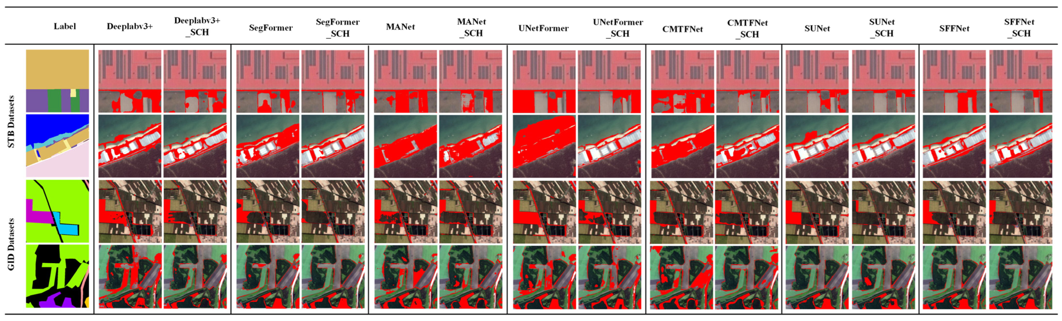
4.4.2. Generalization Analysis

In this part, we conduct an in-depth analysis of the proposed method’s performance across various network architectures by applying it to several deep learning networks, including SegFormer [50], UNetFormer [51], MANet [19], CMTFNet [52], SUNet [53], and SFFNet [54]. SegFormer employs an improved Transformer structure as the encoder to capture long-range dependencies and global contextual information in images. The decoder directly utilizes these features for segmentation without the need for complex post-processing modules. UNetFormer is based on the classic UNet architecture and uses ResNet-50 as the backbone for the encoder, introducing Transformer modules in the decoder to further enhance the integration of multi-scale features. MANet and CMTFNet use ResNet-50 as their backbone, but they employ different attention mechanisms in the decoder to effectively fuse multi-scale and multi-level features. SUNet has an overall structure similar to U-Net, with its encoder composed of Swin Transformer and its decoder utilizing reverse Patch Merging (symmetric to the encoding process) to gradually restore spatial resolution. SFFNet utilizes ConvNeXt as the encoder and integrates spatial and frequency domain features in the decoder to enhance segmentation accuracy in remote sensing. Testing the proposed method across these diverse network architectures allows us to more comprehensively validate its broad applicability.

The results in

Table 6. Segmentation accuracies of different models on GID datasets. Bold text indicates that the network achieved higher accuracy through the addition of MTL-SCH.

Encode	Decode	Params (M)	Method	Coarse Level			Fine Level
				OA	MIoU	FWIoU	OA	MIoU	FWIoU
MiT-B5	MLP	84.60	SegFormer	89.63	81.53	81.42	88.09	76.2	78.97
		87.76	SegFormer-SCH	90.37	82.67	82.63	88.57	77.06	79.74
ResNet50	Attention	35.86	MANet	87.82	78.8	78.52	85.92	71.51	75.64
		42.97	MANet-SCH	88.71	80.38	79.93	86.49	72.79	76.53
ResNet50	Transformer	24.24	UNetFormer	87.26	77.96	77.54	84.93	70.31	74.24
		4.98	UNetFormer-SCH	87.61	78.5	78.17	86.03	72.31	75.84
ResNet50	Attention	30.75	CMTFNet	87.37	76.66	77.78	86.20	71.90	76.03
		36.64	CMTFNet -SCH	89.00	80.77	80.36	87.07	74.45	77.43
Swin Transformer	Swin Transformer	31.82	SUNet	90.94	83.29	83.55	89.95	79.55	81.94
		36.12	SUNet-SCH	91.91	85.25	85.17	90.54	81.41	82.92
ConvNext	Spatial and Frequency Domain Fusion	34.18	SFFNet	92.49	86.26	86.16	91.79	82.57	84.95
		34.35	SFFNet-SCH	93.45	87.81	87.79	92.44	84.48	86.06

indicate that the MTL-SCH method outperforms the STL method in segmentation tasks on the GID dataset. Notably, CMTFNet-SCH shows the greatest improvement at both coarse and fine levels, with a significant increase of 2.55% in mIoU at the fine-level. OA increases from 87.37% to 89.00% at the coarse level, while mIoU increases from 76.66% to 80.77%. Other networks also show varying degrees of improvement in classification accuracy after incorporating MTL-SCH. As shown in Table 6, SegFormer achieves the highest accuracy among all models but shows the smallest improvement after incorporating the proposed method. This may be due to its simple decoder design, which uses an MLP structure, limiting its ability to independently optimize task performance. These results further highlight the advantages of the MTL-SCH method in enhancing land cover classification accuracy and cross-level semantic consistency.

Table 6 shows the parameter counts for each model. STL requires training a separate complete network for each task, whereas MTL-SCH avoids redundant computations by sharing the encoder. Although the total number of parameters in MTL-SCH is slightly higher compared to STL, its ability to generate predictions for both semantic segmentation tasks in a single forward pass significantly reduces computational overhead and improves inference efficiency.

To intuitively compare the effectiveness of the proposed method, examples of different models on GID dataset, along with corresponding VHR images and land cover labels at both coarse and fine levels, are illustrated in Figure 7. Overall, the MTL-SCH method correctly classifies the majority of pixels at both coarse and fine levels compared to the STL method. In Figure 7a, all STL methods exhibit significant semantic inconsistency. For instance, MANet classifies the circled area as forest at the coarse level but incorrectly assigns it to a subclass within the forest category at the fine level, producing a misclassification. In contrast, the MANet-SCH method accurately categorizes this area into the forest subclass at the fine-level, achieving correct classification at both semantic levels and providing better edge handling. Other networks also show improved visual effects at different levels after employing the MTL-SCH method. This indicates that our method effectively alleviates semantic ambiguity and significantly enhances classification accuracy.

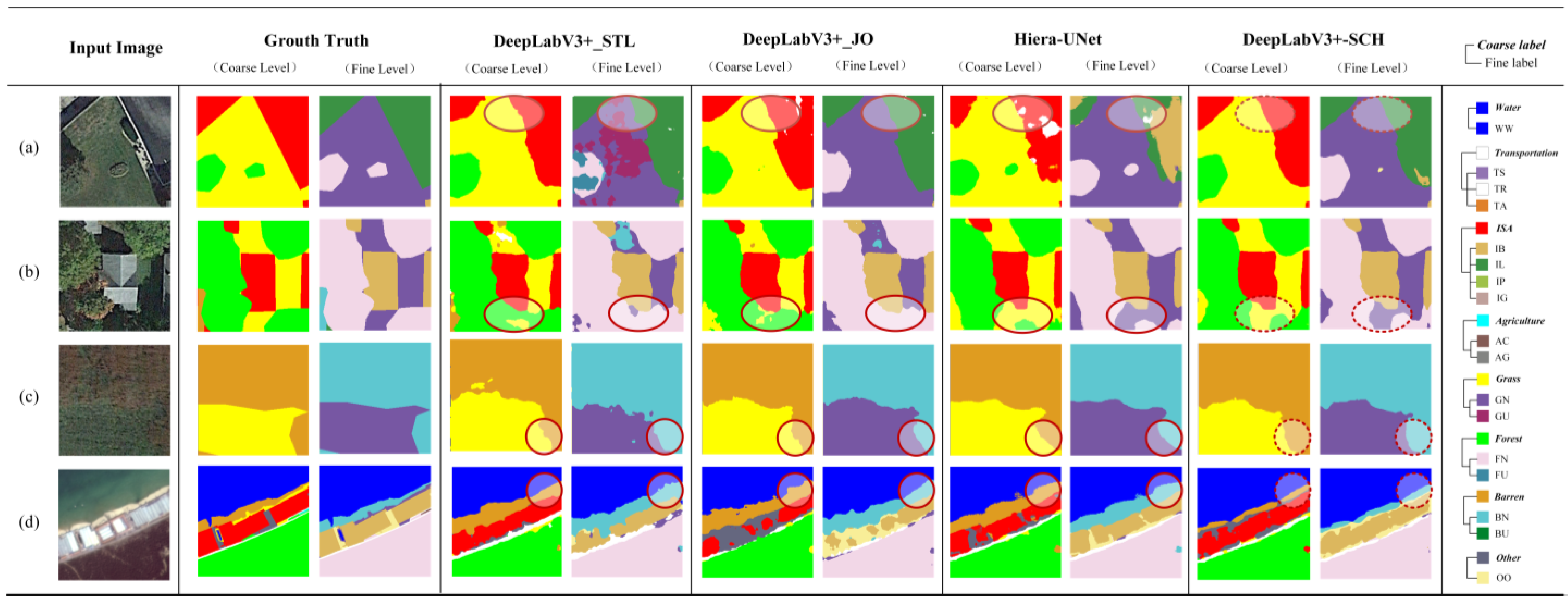
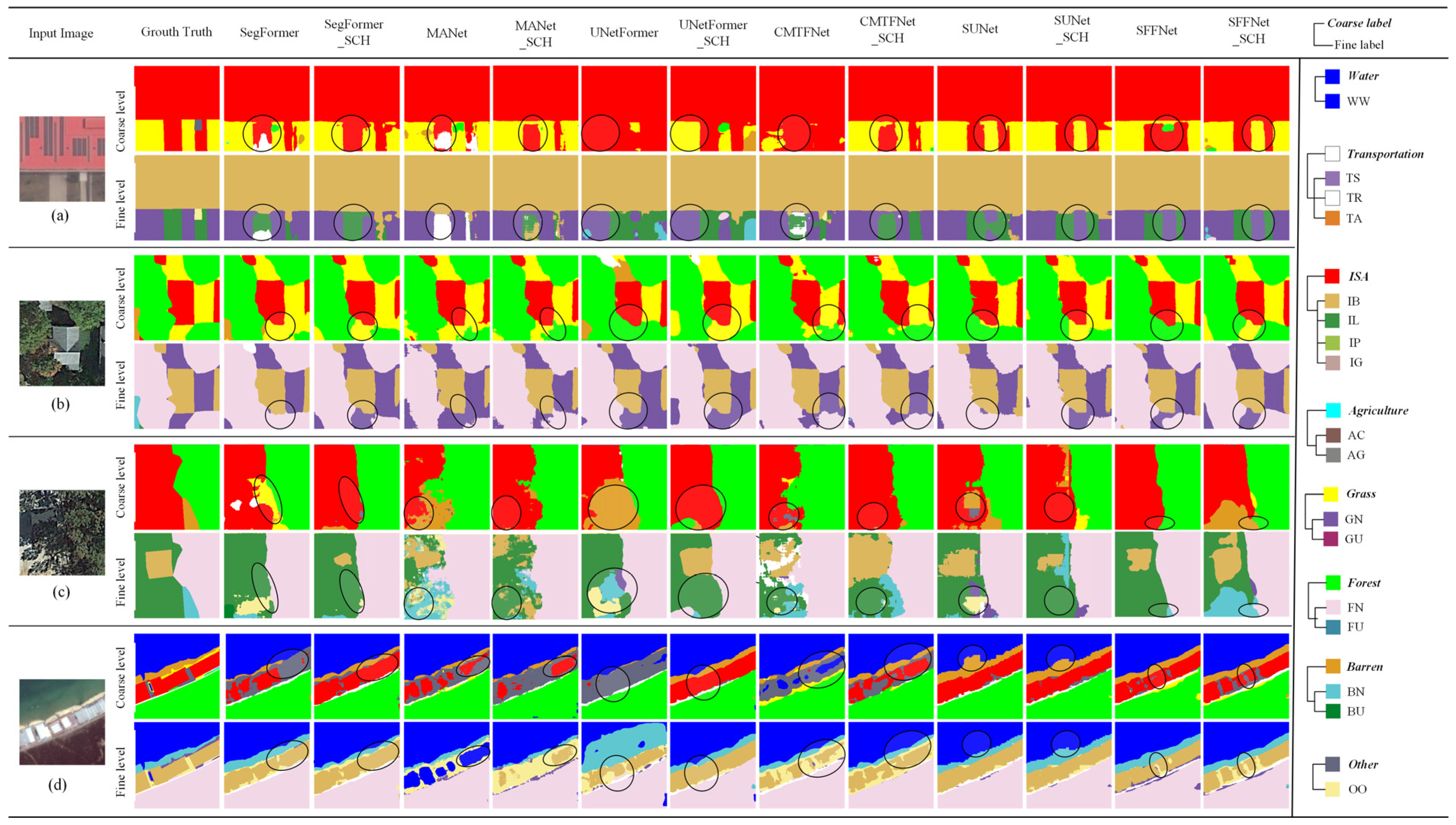
4.5. Experiments on the STB Dataset

To prove the feasibility of the proposed MTL-SCH, we conducted experiments on the STB dataset and compared it to other segmentation methods.

Table 7. Segmentation accuracies of different models on STB datasets. Bold text indicates that the network achieved higher accuracy through the addition of MTL-SCH.

Method	Coarse Level			Fine Level
	OA	MIoU	FWIoU	OA	MIoU	FWIoU
DeepLabv3+_STL	79.27	60.71	66.26	75.79	46.23	61.84
DeepLabv3+_JO	77.98	58.67	64.36	73.78	43.99	59.16
HierU-Net	77.85	59.07	64.60	74.15	43.57	60.01
DeepLabv3+-SCH	80.38	62.90	67.83	77.03	48.22	63.48
SegFormer	77.39	57.56	63.68	72.35	41.86	57.51
SegFormer-SCH	78.40	59.40	64.99	74.13	43.73	59.40
MANet	75.77	55.86	61.50	71.15	39.64	56.05
MANet-SCH	76.61	56.95	62.70	71.76	41.24	57.07
UNetFormer	76.11	55.70	62.29	71.81	41.72	57.42
UNetFormer-SCH	78.81	60.08	65.77	74.69	44.39	60.63
CMTFNet	76.93	57.45	63.28	73.21	43.19	58.73
CMTFNet -SCH	78.56	59.66	65.43	73.92	43.58	59.45
SUNet	79.93	61.55	67.23	77.54	48.72	64.17
SUNet-SCH	81.71	65.15	69.75	78.41	50.02	65.37
SFFNet	80.72	62.73	68.27	77.85	48.75	64.45
SFFNet-SCH	81.46	64.24	69.37	78.36	49.88	65.27

presents the accuracy evaluation results of different methods on the STB dataset. Compared to the DeepLabv3+ model, DeepLabv3+-SCH improves mIoU by 2.19% and 1.99% at the coarse and fine levels, respectively. At the fine level, it outperforms DeepLabv3+_JO and HierU-Net by 4.23% and 4.65% in mIoU, respectively. MTL-SCH is also applied to SegFormer, MANet, UNetFormer, CMTFNet, SUNet, and SFFNet models, achieving mIoU improvements of 1.84%, 0.8%, 4.38%, 2.21%, 3.6%, and 1% at the coarse level and 1.87%, 0.9%, 2.67%, 0.39%, 1.3%, and 1.18% at the fine level. Notably, SUNet-SCH achieves the highest mIoU at both the coarse and fine levels, reaching 65.15% and 50.02%, respectively.

The segmentation examples shown in Figure 8 highlight the advantages of DeepLabv3+-SCH over other methods, improving classification accuracy and enhancing semantic consistency. In contrast, the DeepLabv3+_STL and DeepLabv3+_JO methods produce internal holes and salt-and-pepper noise due to misclassification in the segmentation results. Although HierU-Net improves edge handling, its semantic consistency is still lower than that of other methods. Figure 9 presents the visual classification results of applying MTL-SCH to other models. Overall, the application of the proposed MTL-SCH to other STL models generates more precise segmentation maps, validating the effectiveness of the hierarchical-based land cover mapping method.

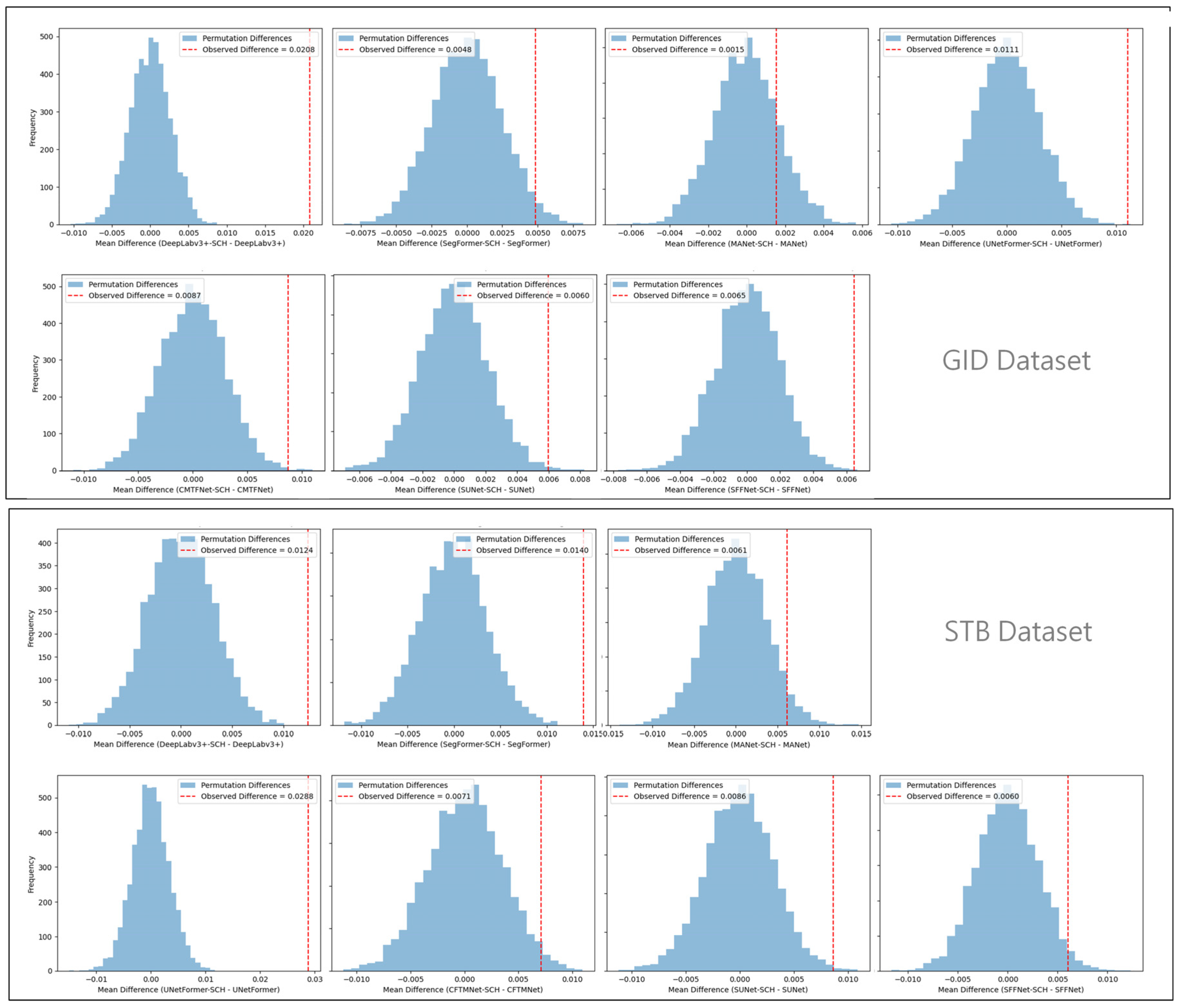
4.6. Statistical Significance Analysis

To assess the reliability of the improvements introduced by MTL-SCH, we conducted statistical significance tests using the permutation test [56], a non-parametric method well-suited for paired comparisons. The test was applied to per-class IoU values on the GID and STB datasets at fine levels, comparing each baseline model with its MTL-SCH-enhanced version. The null hypothesis assumes no performance difference, while the alternative hypothesis posits that MTL-SCH yields significant improvements.

Table 8. Statistical significance analysis of MTL-SCH vs. baseline models.

Backbone Model	GID Dataset			STB Dataset
	mIoU Difference	p-Value	Significant (p < 0.05)	mIoU Difference	p-Value	Significant (p < 0.05)
DeepLabv3+	3.72	<0.0001	✓	1.99	<0.0001	✓
SegFormer	0.86	0.0244	✓	1.87	<0.0001	✓
MANet	1.28	0.1712	✗	0.9	0.0438	✓
UNetFormer	2.00	0.0002	✓	2.67	<0.0001	✓
CMTFNet	2.55	0.0018	✓	0.39	0.0214	✓
SUNet	1.86	0.0040	✓	1.82	0.0030	✓
SFFNet	1.91	0.0002	✓	1.13	0.0222	✓

summarizes the p-values of the statistical tests for each model. As shown, the performance gains brought by MTL-SCH are statistically significant (p < 0.05) for most networks, including DeepLabv3+, SegFormer, UNetFormer, SUNet, and CMTFNet. However, for MANet, the observed improvement in mIoU was relatively small, and the p-value exceeds the 0.05 threshold, indicating that the improvement is not statistically significant. This may be due to the limited sensitivity of MANet’s decoder structure to hierarchical guidance. Figure 10 presents the permutation test distribution plots, where the blue histograms represent the permutation differences, and the red dashed lines indicate the observed difference. On the GID dataset, the observed difference for DeepLabv3+, SegFormer, UNetFormer, CMTFNet, SUNet, and SFFNet significantly deviate from the distribution center, with p-values less than 0.05, confirming that MTL-SCH significantly improves the performance of these models. On the STB dataset, the observed differences for all models demonstrate statistical significance. These results consistently support the effectiveness of MTL-SCH across most models.

4.7. Semantic Consistency Analysis

Semantic consistency ensures that labels at different levels remain aligned, thereby minimizing errors in classification. In this chapter, we comprehensively evaluate the performance of various models and methods regarding semantic consistency on the STB and GID datasets, combining quantitative and qualitative analyses. SAD measures the level of conflict between different semantic levels, whereas ESAD integrates both hierarchical and label conflicts, offering a more comprehensive assessment of the model’s overall performance.

Table 9. Two evaluation metrics for assessing semantic consistency. Bold values denote reduced semantic ambiguity after adding MTL-SCH to the network. The metrics that are highlighted in bold, and red represents the models with the most significant improvements among all models.

Method	STB Dataset		GID Dataset
	SAD (%)	ESAD (%)	SAD (%)	ESAD (%)
DeepLabv3+	14.22	29.71	12.06	21.07
DeepLabv3+-SCH	4.45	24.62	2.21	12.52
Difference	9.77	5.09	9.85	8.55
SegFormer	17.56	33.59	5.90	14.12
SegFormer-SCH	1.92	26.55	1.37	11.71
Difference	15.64	7.04	4.53	2.41
MANet	18.09	35.38	9.37	18.57
MANet-SCH	7.40	30.96	3.63	15.98
Difference	10.69	4.42	5.74	2.59
UNetFormer	18.45	35.24	11.6	20.47
UNetFormer-SCH	4.87	27.09	4.59	16.42
Difference	13.58	8.15	7.01	4.05
CMTFNet	20.23	37.2	9.99	18.99
CMTFNet-SCH	11.28	30.93	3.79	14.74
Difference	8.95	6.27	6.2	4.25
SUNet	14.52	28.8	6.92	13.56
SUNet-MTL	2.83	22.62	1.61	10.18
Difference	11.69	6.18	5.31	3.38
SFFNet	14.46	27.91	6.00	10.88
SFFNet-SCH	1.61	22.26	0.45	7.78
Difference	12.85	5.65	5.55	3.1

shows the SAD and ESAD values of different models on the two datasets.

On the STB dataset, all models showed a more than 8.95% reduction in the SAD metric, indicating significant progress in reducing semantic conflicts between different levels. The SegFormer had the most significant drop in SAD, reaching 15.64%, but did not perform the best in ESAD. This indicates that the model is capable of classifying pixels into semantically consistent levels, but there are still some errors in classification accuracy at different levels. The UNetFormer model performed outstandingly in the ESAD metric, reducing it by 8.15%, which indicates that the introduction of MTL-SCH effectively reduced semantic bias, while improving classification accuracy. On the GID dataset, the DeeplabV3+-SCH model shows the most significant reduction in SAD and ESAD values. It suggests that its structural design is particularly adept at handling the semantic relationships between different levels and facilitates a dual enhancement of semantic consistency and classification accuracy.

The visual results in Figure 11 show that, compared to the STL model, all MTL-SCH models show a significant reduction in pixels with label conflicts. Notably, combination complex decoding structures and hierarchical loss in the Deeplabv3+ and UNetFormer greatly enhances their ability to manage multi-level semantics, resulting in higher classification accuracy and consistency. In contrast, the attention mechanism of MANet may have yet to fully leverage the hierarchical loss optimization within the MTL-SCH framework, leading to a lack of significant improvement in classification consistency. The MTL-SCH framework proves highly effective in enhancing semantic consistency across different levels and improving overall classification performance, though the degree of adaptability varies across different models.

5. Discussion and Conclusions

5.1. Discussion

Experimental results highlight the primary advantage of the MTL-SCH framework, i.e., its ability to enhance both segmentation accuracy and semantic consistency, particularly in maintaining coherence between coarse- and fine-grained categories in multi-level land cover classification. Compared to single-task learning networks (STL), MTL-SCH can generate classification results for two semantic levels using a single model, significantly reducing the number of models and computational redundancy, while improving overall processing efficiency. This advantage stems from fundamental differences in optimization strategies between MTL-SCH and STL. In STL, classification tasks at different levels are optimized independently, often leading to spatially uneven accuracy improvements, with different regions benefiting at different levels. Consequently, even if segmentation accuracy improves, cross-level semantic consistency may remain suboptimal due to misaligned classification boundaries. In contrast, MTL-SCH employs a shared encoder and hierarchical cues to guide joint optimization, ensuring that accuracy gains are more uniformly distributed across levels. This demonstrates the effectiveness of MTL-SCH in hierarchical classification tasks and addresses limitations that conventional segmentation metrics often fail to capture.

However, despite its strengths, MTL-SCH exhibits several limitations that warrant further discussion. First, the model’s performance remains closely tied to the quality of the underlying backbone architecture. For instance, as shown in Figure 10, the SUNet model in the MTL-SCH output still exhibits jagged edges similar to those in the STL output. This is primarily due to the model’s use of Swin Transformer as the backbone network for feature extraction, which is prone to producing such artifacts. This suggests that the hierarchical learning strategy cannot fully overcome the inherent limitations of low-level feature extraction. Future work may explore integrating structure-aware modules (e.g., boundary refinement or edge-enhancement branches) into the backbone or decoder or designing MTL-SCH-compatible lightweight backbones that explicitly preserve spatial details.

Second, a notable trade-off arises between maintaining semantic consistency and achieving optimal classification accuracy at individual levels. The model’s objective to enforce hierarchical alignment may sometimes override pixel-level precision. In extreme cases, as shown in Figure 9c with SFFNet, the outputs maintain cross-level consistency, yet both the coarse and fine categories are misclassified, suggesting that consistency-aware optimization may occasionally bias the model toward structure over correctness. To address this, future research could consider developing adaptive loss weighting mechanisms that dynamically adjust the importance of consistency versus accuracy based on spatial context or prediction uncertainty, thereby achieving a better balance between semantic structure and per-level precision.

Third, although MTL-SCH demonstrates generalizability across different backbones, its integration into existing architectures requires structural modifications, such as the addition of dual decoders and hierarchical loss modules, which may reduce its ease of deployment in real-world systems. Additionally, a notable limitation is the increased parameter count, which could elevate memory and computational demands. To address these challenges, future studies could explore plug-and-play versions of MTL-SCH that leverage shared output heads or lightweight hierarchical regularization modules. These adaptations would minimize architectural intrusion and parameter overhead, while preserving the benefits of cross-level consistency.

In summary, MTL-SCH provides moderate improvements in classification accuracy while demonstrating significant advantages in enhancing cross-level semantic consistency. It offers a unified solution for generating multi-level classification results and addresses key limitations of traditional flat or isolated classification approaches. Although challenges remain, including backbone dependency, consistency–accuracy trade-offs, and architectural complexity, these open questions offer rich directions for further investigation.

5.2. Conclusions

This paper introduces a multi-level land cover mapping method based on a deep multi-task learning (MTL) framework. The MTL-SCH method treats coarse and fine-levels land cover classifications as interrelated yet independent tasks, addressing the semantic inconsistency caused by the isolated handling of different semantic levels in traditional methods. This approach effectively mitigates error propagation and achieves synchronized optimization of classification results at each level. MTL-SCH facilitates information exchange between tasks, while preserving the independence and specificity of each task through shared feature representations and a cascading mechanism. Additionally, the framework explicitly models the dependencies between coarse and fine-levels through the loss function, further enhancing the alignment between different semantic levels and ensuring cross-level semantic consistency.

This study validated the proposed MTL-SCH method on the STB and GID datasets, demonstrating its adaptability across various deep-learning network architectures. Whether applied to models such as CNN, Transformer, or CNN-Former, the framework consistently achieved performance improvements, indicating that MTL-SCH is suitable for a single network structure and possesses broad transferability. By overcoming the limitations of traditional planar segmentation models, the MTL-SCH provides an innovative solution for achieving the dual optimization of semantic alignment and fine classification, paving the way for new application prospects in remote sensing-based land use and land cover monitoring.

References

1. Wu, F.; Wang, C.; Zhang, H.; Li, J.; Li, L.; Chen, W.; Zhang, B. Built-up area mapping in China from GF-3 SAR imagery based on the framework of deep learning. Remote Sens. Environ. 2021, 262, 112515. [Google Scholar] [CrossRef]
2. Albarakati, H.M.; Khan, M.A.; Hamza, A.; Khan, F.; Kraiem, N.; Jamel, L.; Almuqren, L.; Alroobaea, R. A Novel Deep Learning Architecture for Agriculture Land Cover and Land Use Classification from Remote Sensing Images Based on Network-Level Fusion of Self-Attention Architecture. IEEE J. Sel. Top. Appl. Earth Obs. Remote Sens. 2024, 17, 6338–6353. [Google Scholar] [CrossRef]
3. Zhang, H.; Zheng, J.; Hunjra, A.I.; Zhao, S.; Bouri, E. How Does Urban Land Use Efficiency Improve Resource and Environment Carrying Capacity? Socio-Econ. Plan. Sci. 2024, 91, 101760. [Google Scholar] [CrossRef]
4. Anderson, J.R. A Land Use and Land Cover Classification System for Use with Remote Sensor Data; US Government Printing Office: Colorado, CO, USA, 1976.
5. Bossard, M.; Feranec, J.; Otahel, J. CORINE Land Cover Technical Guide: Addendum 2000; European Environment Agency Copenhagen: Denmark, Copenhagen, 2000. [Google Scholar]
6. Di Gregorio, A. Land Cover Classification System: Classification Concepts and User Manual: LCCS; Food & Agriculture Org: Rome, Italy, 2005. [Google Scholar]
7. Zafari, A.; Zurita-Milla, R.; Izquierdo-Verdiguier, E. Land Cover Classification Using Extremely Randomized Trees: A Kernel Perspective. IEEE Geosci. Remote Sens. Lett. 2019, 17, 1702–1706. [Google Scholar] [CrossRef]
8. Tatsumi, K.; Yamashiki, Y.; Torres, M.A.C.; Taipe, C.L.R. Crop Classification of Upland Fields Using Random Forest of Time-Series Landsat 7 ETM+ Data. Comput. Electron. Agric. 2015, 115, 171–179. [Google Scholar] [CrossRef]
9. Zhang, C.; Pan, X.; Li, H.; Gardiner, A.; Sargent, I.; Hare, J.; Atkinson, P.M. A Hybrid MLP-CNN Classifier for Very Fine Resolution Remotely Sensed Image Classification. ISPRS J. Photogramm. Remote Sens. 2018, 140, 133–144. [Google Scholar] [CrossRef]
10. Li, J.; Zhang, B.; Huang, X. A Hierarchical Category Structure Based Convolutional Recurrent Neural Network (HCS-ConvRNN) for Land-Cover Classification Using Dense MODIS Time-Series Data. Int. J. Appl. Earth Obs. Geoinf. 2022, 108, 102744. [Google Scholar] [CrossRef]
11. Gavish, Y.; O’Connell, J.; Marsh, C.J.; Tarantino, C.; Blonda, P.; Tomaselli, V.; Kunin, W.E. Comparing the Performance of Flat and Hierarchical Habitat/Land-Cover Classification Models in a NATURA 2000 Site. ISPRS J. Photogramm. Remote Sens. 2018, 136, 1–12. [Google Scholar] [CrossRef]
12. Demirkan, D.Ç.; Koz, A.; Düzgün, H.Ş. Hierarchical Classification of Sentinel 2-a Images for Land Use and Land Cover Mapping and Its Use for the CORINE System. J. Appl. Remote Sens. 2020, 14, 026524. [Google Scholar] [CrossRef]
13. Yang, C.; Rottensteiner, F.; Heipke, C. Exploring Semantic Relationships for Hierarchical Land Use Classification Based on Convolutional Neural Networks. ISPRS Ann. Photogramm. Remote Sens. Spat. Inf. Sci. 2020, 2, 599–607. [Google Scholar] [CrossRef]
14. Waśniewski, A.; Hościło, A.; Chmielewska, M. Can a Hierarchical Classification of Sentinel-2 Data Improve Land Cover Mapping? Remote Sens. 2022, 14, 989. [Google Scholar] [CrossRef]
15. Sulla-Menashe, D.; Friedl, M.A.; Krankina, O.N.; Baccini, A.; Woodcock, C.E.; Sibley, A.; Sun, G.; Kharuk, V.; Elsakov, V. Hierarchical Mapping of Northern Eurasian Land Cover Using MODIS Data. Remote Sens. Environ. 2011, 115, 392–403. [Google Scholar] [CrossRef]
16. Gong, P.; Wang, J.; Yu, L.; Zhao, Y.; Zhao, Y.; Liang, L.; Niu, Z.; Huang, X.; Fu, H.; Liu, S.; et al. Finer Resolution Observation and Monitoring of Global Land Cover: First Mapping Results with Landsat TM and ETM+ Data. Int. J. Remote Sens. 2013, 34, 2607–2654. [Google Scholar] [CrossRef]
17. Zhang, X.; Liu, L.; Chen, X.; Gao, Y.; Xie, S.; Mi, J. GLC_FCS30: Global Land-Cover Product with Fine Classification System at 30 m Using Time-Series Landsat Imagery. Earth Syst. Sci. Data Discuss. 2020, 2020, 2753–2776. [Google Scholar] [CrossRef]
18. Xie, S.; Liu, L.; Zhang, X.; Yang, J.; Chen, X.; Gao, Y. Automatic Land-Cover Mapping Using Landsat Time-Series Data Based on Google Earth Engine. Remote Sens. 2019, 11, 3023. [Google Scholar] [CrossRef]
19. Li, R.; Zheng, S.; Zhang, C.; Duan, C.; Su, J.; Wang, L.; Atkinson, P.M. Multiattention Network for Semantic Segmentation of Fine-Resolution Remote Sensing Images. IEEE Trans. Geosci. Remote Sens. 2022, 60, 5607713. [Google Scholar] [CrossRef]
20. TANG, B.; PALIDAN, T.; BAI, J.; QI, R. Land Cover Classification Method for Remote Sensing Images Using CNN and Transformer. Microelectron. Comput. 2024, 41, 64–73. [Google Scholar]
21. Xia, J.; Yokoya, N.; Adriano, B.; Broni-Bediako, C. Openearthmap: A Benchmark Dataset for Global High-Resolution Land Cover Mapping. In Proceedings of the IEEE/CVF Winter Conference on Applications of Computer Vision, Tucson, AZ, USA, 2–7 January 2023; pp. 6254–6264. [Google Scholar] [CrossRef]
22. Tong, X.-Y.; Xia, G.-S.; Lu, Q.; Shen, H.; Li, S.; You, S.; Zhang, L. Land-Cover Classification with High-Resolution Remote Sensing Images Using Transferable Deep Models. Remote Sens. Environ. 2020, 237, 111322. [Google Scholar] [CrossRef]
23. ISPRS Potsdam 2D Semantic Labeling Dataset. Available online: https://www.isprs.org/resources/datasets/benchmarks/UrbanSemLab/2d-sem-label-potsdam.aspx (accessed on 22 December 2021).
24. ISPRS Vaihingen 2D Semantic Labeling Dataset. Available online: https://www.isprs.org/resources/datasets/benchmarks/UrbanSemLab/2d-sem-label-vaihingen.aspx (accessed on 22 December 2021).
25. Fu, Y.; Zhang, X.; Wang, M. DSHNet: A Semantic Segmentation Model of Remote Sensing Images Based on Dual Stream Hybrid Network. IEEE J. Sel. Top. Appl. Earth Obs. Remote Sens. 2024, 17, 4164–4175. [Google Scholar] [CrossRef]
26. Cao, Y.; Huo, C.; Xiang, S.; Pan, C. GFFNet: Global Feature Fusion Network for Semantic Segmentation of Large-Scale Remote Sensing Images. IEEE J. Sel. Top. Appl. Earth Obs. Remote Sens. 2024, 17, 4222–4234. [Google Scholar] [CrossRef]
27. Yang, K.; Tong, X.-Y.; Xia, G.-S.; Shen, W.; Zhang, L. Hidden Path Selection Network for Semantic Segmentation of Remote Sensing Images. IEEE Trans. Geosci. Remote Sens. 2022, 60, 5628115. [Google Scholar] [CrossRef]
28. Li, Z.; Bao, W.; Zheng, J.; Xu, C. Deep Grouping Model for Unified Perceptual Parsing. In Proceedings of the IEEE/CVF Conference on Computer Vision and Pattern Recognition, Los Alamitos, CA, USA, 14–19 June 2020; pp. 4053–4063. [Google Scholar] [CrossRef]
29. Liang, X.; Xing, E.; Zhou, H. Dynamic-Structured Semantic Propagation Network. In Proceedings of the 2018 IEEE/CVF Conference on Computer Vision and Pattern Recognition, Salt Lake City, UT, USA, 18–23 June 2018; pp. 752–761. [Google Scholar]
30. Deng, J.; Ding, N.; Jia, Y.; Frome, A.; Murphy, K.; Bengio, S.; Li, Y.; Neven, H.; Adam, H. Large-Scale Object Classification Using Label Relation Graphs. In Proceedings of the Computer Vision–ECCV 2014: 13th European Conference, Zurich, Switzerland, 6–12 September 2014; pp. 48–64. [Google Scholar] [CrossRef]
31. Chen, J.; Qian, Y. Hierarchical Multi-Label Ship Recognition in Remote Sensing Images Using Label Relation Graphs. In Proceedings of the 2021 IEEE International Geoscience and Remote Sensing Symposium IGARSS, Brussels, Belgium, 11–16 July 2021; pp. 4968–4971. [Google Scholar] [CrossRef]
32. Zhang, X.; Hong, W.; Li, Z.; Cheng, X.; Tang, X.; Zhou, H.; Jiao, L. Hierarchical Knowledge Graph for Multilabel Classification of Remote Sensing Images. IEEE Trans. Geosci. Remote Sens. 2024, 62, 5645714. [Google Scholar] [CrossRef]
33. Jo, S.; Shin, D.; Na, B.; Jang, J.; Moon, I.-C. Hierarchical Multi-Label Classification with Partial Labels and Unknown Hierarchy. In Proceedings of the 32nd ACM International Conference on Information and Knowledge Management, Birmingham UK, 21–25 October 2023; pp. 1025–1034. [Google Scholar] [CrossRef]
34. Patel, D.; Dangati, P.; Lee, J.-Y.; Boratko, M.; McCallum, A. Modeling Label Space Interactions in Multi-Label Classification Using Box Embeddings. ICLR 2022 Poster 2022. [Google Scholar]
35. Giunchiglia, E.; Lukasiewicz, T. Coherent Hierarchical Multi-Label Classification Networks. Adv. Neural Inf. Process. Syst. 2020, 33, 9662–9673. [Google Scholar]
36. Li, L.; Zhou, T.; Wang, W.; Li, J.; Yang, Y. Deep Hierarchical Semantic Segmentation. In Proceedings of the 2022 IEEE/CVF Conference on Computer Vision and Pattern Recognition (CVPR), New Orleans, LA, USA, 18–24 June 2022; pp. 1236–1247. [Google Scholar] [CrossRef]
37. Sulla-Menashe, D.; Gray, J.M.; Abercrombie, S.P.; Friedl, M.A. Hierarchical Mapping of Annual Global Land Cover 2001 to Present: The MODIS Collection 6 Land Cover Product. Remote Sens. Environ. 2019, 222, 183–194. [Google Scholar] [CrossRef]
38. Liu, L.; Tong, Z.; Cai, Z.; Wu, H.; Zhang, R.; Le Bris, A.; Olteanu-Raimond, A.-M. HierU-Net: A Hierarchical Semantic Segmentation Method for Land Cover Mapping. IEEE Trans. Geosci. Remote Sens. 2024, 62, 4404614. [Google Scholar] [CrossRef]
39. Yang, C.; Rottensteiner, F.; Heipke, C. A Hierarchical Deep Learning Framework for the Consistent Classification of Land Use Objects in Geospatial Databases. ISPRS J. Photogramm. Remote Sens. 2021, 177, 38–56. [Google Scholar] [CrossRef]
40. Gbodjo, Y.J.E.; Ienco, D.; Leroux, L.; Interdonato, R.; Gaetano, R.; Ndao, B. Object-Based Multi-Temporal and Multi-Source Land Cover Mapping Leveraging Hierarchical Class Relationships. Remote Sens. 2020, 12, 2814. [Google Scholar] [CrossRef]
41. Zhang, Y.; Yang, Q. A Survey on Multi-Task Learning. IEEE Trans. Knowl. Data Eng. 2021, 34, 5586–5609. [Google Scholar] [CrossRef]
42. Kokkinos, I. Ubernet: Training a Universal Convolutional Neural Network for Low-, Mid-, and High-Level Vision Using Diverse Datasets and Limited Memory. In Proceedings of the IEEE conference on computer vision and pattern recognition, Honolulu, HI, USA, 21–26 July 2017; pp. 6129–6138. [Google Scholar]
43. Xu, D.; Ouyang, W.; Wang, X.; Sebe, N. Pad-Net: Multi-Tasks Guided Prediction-and-Distillation Network for Simultaneous Depth Estimation and Scene Parsing. In Proceedings of the IEEE Conference on Computer Vision and Pattern Recognition, Salt Lake City, UT, USA, 18–23 June 2018; pp. 675–684. [Google Scholar]
44. Vandenhende, S.; Georgoulis, S.; Van Gool, L. MTI-Net: Multi-Scale Task Interaction Networks for Multi-Task Learning. In Computer Vision—ECCV 2020; Vedaldi, A., Bischof, H., Brox, T., Frahm, J.-M., Eds.; Lecture Notes in Computer Science; Springer International Publishing: Cham, Switzerland, 2020; Volume 12349, pp. 527–543. [Google Scholar] [CrossRef]
45. Misra, I.; Shrivastava, A.; Gupta, A.; Hebert, M. Cross-Stitch Networks for Multi-Task Learning. In Proceedings of the IEEE Conference on Computer Vision and Pattern Recognition, Las Vegas, NV, USA, 27–30 June 2016; pp. 3994–4003. [Google Scholar] [CrossRef]
46. Ruder, S.; Bingel, J.; Augenstein, I.; Søgaard, A. Latent Multi-Task Architecture Learning. Proc. AAAI Conf. Artif. Intell. 2019, 33, 4822–4829. [Google Scholar] [CrossRef]
47. Liu, S.; Johns, E.; Davison, A.J. End-to-End Multi-Task Learning with Attention. In Proceedings of the IEEE/CVF Conference on Computer Vision and Pattern Recognition, Long Beach, CA, USA, 15–20 June 2019; pp. 1871–1880. [Google Scholar] [CrossRef]
48. Lopes, I.; Vu, T.-H.; de Charette, R. Cross-Task Attention Mechanism for Dense Multi-Task Learning. In Proceedings of the IEEE/CVF Winter Conference on Applications of Computer Vision, Waikoloa, HI, USA, 2–7 January 2023; pp. 2329–2338. [Google Scholar] [CrossRef]
49. Goncalves, D.N.; Marcato, J.; Zamboni, P.; Pistori, H.; Li, J.; Nogueira, K.; Goncalves, W.N. MTLSegFormer: Multi-Task Learning with Transformers for Semantic Segmentation in Precision Agriculture. In Proceedings of the 2023 IEEE/CVF Conference on Computer Vision and Pattern Recognition Workshops (CVPRW), Vancouver, BC, Canada, 17–24 June 2023; pp. 6290–6298. [Google Scholar] [CrossRef]
50. Xie, E.; Wang, W.; Yu, Z.; Anandkumar, A.; Alvarez, J.M.; Luo, P. SegFormer: Simple and Efficient Design for Semantic Segmentation with Transformers. Adv. Neural Inf. Process. Syst. 2021, 34, 12077–12090. [Google Scholar]
51. Wang, L.; Li, R.; Zhang, C.; Fang, S.; Duan, C.; Meng, X.; Atkinson, P.M. UNetFormer: A UNet-like Transformer for Efficient Semantic Segmentation of Remote Sensing Urban Scene Imagery. ISPRS J. Photogramm. Remote Sens. 2022, 190, 196–214. [Google Scholar] [CrossRef]
52. Wu, H.; Huang, P.; Zhang, M.; Tang, W.; Yu, X. CMTFNet: CNN and Multiscale Transformer Fusion Network for Remote-Sensing Image Semantic Segmentation. IEEE Trans. Geosci. Remote Sens. 2023, 61, 2004612. [Google Scholar] [CrossRef]
53. Cao, H.; Wang, Y.; Chen, J.; Jiang, D.; Zhang, X.; Tian, Q.; Wang, M. Swin-Unet: Unet-Like Pure Transformer for Medical Image Segmentation. In Computer Vision—ECCV 2022 Workshops; Karlinsky, L., Michaeli, T., Nishino, K., Eds.; Lecture Notes in Computer Science; Springer Nature: Cham, Switzerland, 2023; Volume 13803, pp. 205–218. [Google Scholar] [CrossRef]
54. Yang, Y.; Yuan, G.; Li, J. Sffnet: A Wavelet-Based Spatial and Frequency Domain Fusion Network for Remote Sensing Segmentation. IEEE Trans. Geosci. Remote Sens. 2024, 62, 3000617. [Google Scholar] [CrossRef]
55. Garcia-Garcia, A.; Orts-Escolano, S.; Oprea, S.; Villena-Martinez, V.; Garcia-Rodriguez, J.A. Review on Deep Learning Techniques Applied to Semantic Segmentation. arXiv 2017, arXiv:1704.06857. [Google Scholar] [CrossRef]
56. Ernst, M.D. Permutation Methods: A Basis for Exact Inference. Stat. Sci. 2004, 19, 676–685. [Google Scholar] [CrossRef]
Figure 1. (a) Hierarchical classification structure for VHR imagery. (b) Top-down and bottom-up methods. Both methods will lead to error propagation issues. (c) Semantic inconsistency. When independent segmentation models are employed for coarse-level and fine-level tasks, it may result in correct coarse-level classifications but erroneous fine-level classifications, thereby leading to issues of semantic inconsistency.
Remotesensing 17 02442 g001
Figure 2. The overall framework of MTL-SCH. (a) Model structure. (b) Hierarchical structure tree. (c) Hierarchical loss calculation process. When v is a positive class, the probability score of the associated node u should exceed or be equal to the probability score of node v (0.8→0.3). When v is a negative class, the probability score of the associated node u should not exceed the probability score of node v (0.4→0.6).
Remotesensing 17 02442 g002
Figure 3. The architecture of the proposed multi-task learning framework (MTL-SCH) based on DeepLabv3+. The encoder extracts low-level and high-level features (yellow boxes in the figure). Two decoders perform coarse and fine-level segmentation tasks, respectively (coarse-level segmentation task is indicated by green boxes, fine-level segmentation task is indicated by blue boxes). Feature concatenation between decoders strengthens hierarchical consistency. The structure of the ASPP module is indicated by purple boxes.
Remotesensing 17 02442 g003
Figure 4. Performance comparison of different method for each class in the coarse and fine category.
Remotesensing 17 02442 g004
Figure 5. Deeplabv3+_STL and Deeplabv3+-SCH confusion matrix heatmap. The red dashed boxes represent the coarse-level categories.
Remotesensing 17 02442 g005
Figure 6. Examples of semantic segmentation results. From left to right are the VHR image, ground truth, and results from Deeplabv3+_STL, Deeplabv3+_JO, HierU-Net, and Deeplabv3+-SCH. (a) DeepLabv3+-SCH achieves more accurate segmentation on the Built-up (superclass) and Industrial Land (subclass) regions. (b) DeepLabv3+-SCH achieves more accurate segmentation on the Built-up (superclass) and Rural Residential (subclass) regions. (c) DeepLabv3+-SCH achieves more accurate segmentation on the Farmland (superclass) and Irrigated Land (subclass) regions. (d) DeepLabv3+-SCH achieves more accurate segmentation on the Forest (superclass) and Arbor Forest (subclass) regions.
Remotesensing 17 02442 g006
Figure 7. Visualized results of different networks on the GID dataset. (a) After applying MTL-SCH, the model achieves more accurate segmentation for the Forest (superclass) and Garden Land (subclass). (b) After applying MTL-SCH, the model achieves more accurate segmentation for the Water (superclass) and River (subclass). (c) After applying MTL-SCH, the model achieves more accurate segmentation for the Built-up (superclass) and Traffic Land (subclass). (d) After applying MTL-SCH, the model achieves more accurate segmentation for the Farmland (superclass) and Irrigated Land (subclass).
Remotesensing 17 02442 g007
Figure 8. Examples of semantic segmentation results on the STB dataset. From left to right are the VHR image, ground truth, and results from Deeplabv3+_STL, Deeplabv3+_JO, HierU-Net, and Deeplabv3+-SCH. (a) DeepLabv3+-SCH achieves more accurate segmentation on the Impervious Surface (superclass) and Parking Lot (subclass) regions. (b) DeepLabv3+-SCH achieves more accurate segmentation on the Grass (superclass) and Natural Grass (subclass) regions. (c) DeepLabv3+-SCH achieves more accurate segmentation on the Barren (superclass) and Natural Bare Soil (subclass) regions. (d) DeepLabv3+-SCH achieves more accurate segmentation on the Water (superclass) and Water (subclass) regions.
Remotesensing 17 02442 g008
Figure 9. Visualized results of different networks on the STB dataset. (a) After applying MTL-SCH, the model achieves more accurate segmentation for the Grass (superclass) and Natural Grass (subclass). (b) After applying MTL-SCH, the model achieves more accurate segmentation for the Grass (superclass) and Natural Grass (subclass). (c) After applying MTL-SCH, the model achieves more accurate segmentation for the Barren (superclass) and Natural Bare Soil (subclass). (d) After applying MTL-SCH, the model achieves more accurate segmentation for the Other (superclass) and Other (subclass).
Remotesensing 17 02442 g009
Figure 10. Statistical significance analysis.
Remotesensing 17 02442 g010
Figure 11. Pixels where label conflicts or hierarchical conflicts occur in the classification results. The transparent areas represent pixels that have consistent semantics and correct classification at both levels, while the red areas indicate pixels with inconsistent semantics (hierarchical conflicts) or incorrect classification (label conflicts).
Remotesensing 17 02442 g011