Multi-Channel Coupled Variational Bayesian Framework with Structured Sparse Priors for High-Resolution Imaging of Complex Maneuvering Targets

Abstract

High-resolution ISAR (Inverse Synthetic Aperture Radar) imaging plays a crucial role in dynamic target monitoring for aerospace, maritime, and ground surveillance. Among various remote sensing techniques, ISAR is distinguished by its ability to produce high-resolution images of non-cooperative maneuvering targets. To meet the increasing demands for resolution and robustness, modern ISAR systems are evolving toward wideband and multi-channel architectures. In particular, multi-channel configurations based on large-scale receiving arrays have gained significant attention. In such systems, each receiving element functions as an independent spatial channel, acquiring observations from distinct perspectives. These multi-angle measurements enrich the available echo information and enhance the robustness of target imaging. However, this setup also brings significant challenges, including inter-channel coupling, high-dimensional joint signal modeling, and non-Gaussian, mixed-mode interference, which often degrade image quality and hinder reconstruction performance. To address these issues, this paper proposes a Hybrid Variational Bayesian Multi-Interference (HVB-MI) imaging algorithm based on a hierarchical Bayesian framework. The method jointly models temporal correlations and inter-channel structure, introducing a coupled processing strategy to reduce dimensionality and computational complexity. To handle complex noise environments, a Gaussian mixture model (GMM) is used to represent nonstationary mixed noise. A variational Bayesian inference (VBI) approach is developed for efficient parameter estimation and robust image recovery. Experimental results on both simulated and real-measured data demonstrate that the proposed method achieves significantly improved image resolution and noise robustness compared with existing approaches, particularly under conditions of sparse sampling or strong interference. Quantitative evaluation further shows that under the continuous sparse mode with a 75% sampling rate, the proposed method achieves a significantly higher Laplacian Variance (LV), outperforming PCSBL and CPESBL by 61.7% and 28.9%, respectively and thereby demonstrating its superior ability to preserve fine image details.

1. Introduction

Inverse Synthetic Aperture Radar (ISAR) technology enables the high-resolution imaging of moving targets under complex environmental conditions, playing a crucial role in long-range detection and precise identification [1,2]. Compared with traditional single-channel imaging modes, modern ISAR systems are increasingly adopting multi-channel configurations to enhance imaging resolution and robustness. In this work, the term multi-channel specifically refers to a large-scale receiving array, where each receiving element functions as an independent spatial channel. This setup enables the collection of echo signals from multiple perspectives, thereby enhancing the system’s ability to resolve fine-scale target features. However, such array-based multi-channel configurations also introduce significant technical challenges, including high-dimensional data coupling, inter-channel correlation, nonstationary noise, and increased computational burden. Conventional ISAR imaging algorithms, which are typically designed for single-channel or simplified systems, often rely on assumptions such as independent noise, uncorrelated observations, or uniform resolution across channels. These methods struggle to cope with the structured and high-dimensional nature of multi-channel data, resulting in substantial performance degradation in practical ISAR scenarios. These issues necessitate the development of sparse modeling frameworks capable of capturing spatiotemporal structures and suppressing complex non-Gaussian interference in real-world environments [3,4].

The core of multi-channel sparse echo signal processing lies in fully exploiting the joint sparsity of echo data to effectively integrate complementary spatiotemporal information, thereby improving motion parameter estimation accuracy and target imaging resolution. For instance, the method proposed in [5] employs multi-channel fusion-based sparse imaging to achieve high-precision reconstruction of stationary targets. However, for targets exhibiting complex motion characteristics, the echo signals often present strong spatiotemporal coupling and are affected by various noise and interference sources, making the imaging process significantly more challenging. Existing algorithms in multi-channel signal processing often fail to fully utilize these characteristics, leading to degraded imaging quality, reduced resolution, and consequently, severe limitations in subsequent target recognition and feature extraction.

Despite various solutions proposed in the literature, current methods still face significant limitations when handling multi-channel signals. First, conventional algorithms such as orthogonal matching pursuit (OMP)and sparse Bayesian learning (SBL) perform well in single-channel scenarios but extend multi-channel data dimensions simply by stacking, increasing the dimensionality by a factor of N (where N is the number of channels). This results in a surge in computational complexity from O(N³) to O(N⁶) [6] while failing to exploit the structured sparsity of maneuvering targets in both fast and slow time dimensions, leading to excessive data redundancy. Second, existing multi-channel extensions, such as M-SBL [7], rely on a fixed covariance matrix to describe channel correlations. However, when a target undergoes complex roll–pitch maneuvers, the time-varying polarization scattering characteristics introduce nonstationary channel correlations. Single-channel approaches oversimplify such maneuvers, and experiments have shown that this simplification leads to a reduction in azimuth resolution. Furthermore, current frameworks assume that noise across channels follows an independent and identically distributed (i.i.d.) Gaussian model, whereas in practical systems, channel-specific multiplicative noise and cross-channel coherent interference coexist [7,8,9]. The spectral density differences of such mixed noise components are significant, which reduces the signal-to-noise ratio (SNR) of weak scatterer reconstruction. These deficiencies stem from an insufficient understanding of multi-channel coupling mechanisms in existing methods [10].

The rapid maneuvers of complex moving targets produce time-varying cross-channel coupling effects in both the fast and slow time dimensions, which make it difficult to process complex multi-channel information and significantly affect imaging resolution. However, current methods only process multi-channel information by superimposing high-dimensional data, without considering the nonstationary correlations in multi-channels under complex motion scenes, nor establishing a robust imaging model for mixed noise characteristics. Therefore, achieving collaborative optimization of efficient high-dimensional signal processing, accurate modeling of nonstationary correlations, and joint suppression of mixed noise interference has become a key challenge in improving the accuracy of sparse imaging.

Thus, existing sparse sensing-based imaging methods can be broadly classified into three categories: greedy algorithms, convex optimization methods, and Bayesian approaches [10]. Greedy algorithms iteratively select the atom with the highest residual by constructing a complete dictionary, progressively reconstructing the target image. While computationally efficient, they often fail to effectively exploit inter-channel correlations and sparsity in multi-channel data processing, leading to lower imaging accuracy and robustness. This limitation is particularly evident in the imaging of complex moving targets, where their performance tends to be unstable [11,12]. Convex optimization methods achieve efficient target image reconstruction by imposing regularization constraints. However, the selection of the regularization parameter typically relies on empirical tuning. Moreover, in multi-channel signal processing, these methods struggle to fully exploit inter-channel joint sparsity, limiting their adaptability to dynamic target imaging [13].

Early work by Li and Stoical played a foundational role in the development of SBL and expectation maximization (EM)-based inference techniques, which have been applied in radar imaging [14,15]. This method introduced inference mechanisms that significantly advanced the field of sparse signal processing and continue to serve as the basis for many modern extensions.

Bayesian approaches, on the other hand, integrate prior distributions with the observation model, demonstrating greater flexibility, particularly in multi-channel echo data processing. Multi-channel echo data provide richer information, and Bayesian methods leverage both sparsity and inter-channel correlations to enhance imaging accuracy and robustness [16,17,18,19]. Compared to other approaches, Bayesian methods are better suited to accommodate the complex motion characteristics of dynamic targets, offering superior imaging precision and reconstruction performance.

As the complexity of target motion increases, the limitations of traditional Bayesian methods become more pronounced. SBL [5] effectively utilizes the inherent uncertainty of echo signals to generate high-precision ISAR images. However, since each iteration requires solving an N × N matrix, its computational complexity is O(N³) [20], which becomes even more critical in multi-channel data processing. To address this, a high-resolution ISAR imaging technique based on hierarchical SBL was proposed in [21], incorporating sparse priors to reconstruct missing data. However, its reconstruction accuracy for complex moving targets remains limited. To further refine the model, researchers have introduced gamma-Gaussian distributions [22] and gamma-complex Gaussian distributions [23] to improve modeling accuracy. Additionally, Bayesian inference was applied in [24] for precise parameter estimation, but its reconstruction accuracy deteriorates when applied to complex moving targets, leading to localized imaging blurring.

Most existing Bayesian parameter estimation methods still rely on single-channel echo data modeling and often suffer from high computational complexity. Recent studies have sought to address this challenge. For instance, ref. [25] proposed one-dimensional and two-dimensional non-invertible fast Bayesian inference methods, while [26] developed the ADMM-SBL method specifically designed for gamma-complex Gaussian distributions to alleviate computational burdens. However, these methods remain constrained to single-channel signal processing, limiting their flexibility in dynamic target scenarios. Due to the intricate motion patterns of dynamic targets, traditional methods struggle to effectively capture the temporal coupling and time-varying characteristics of echo data, ultimately affecting imaging accuracy and robustness. Consequently, to better capture the motion characteristics of dynamic targets, sensing imaging systems are evolving toward wider bandwidths and multi-channel configurations, leveraging additional echo data and observational information to enhance image reconstruction accuracy and robustness.

Unlike traditional single-channel sensing imaging methods, multi-channel configurations provide richer observational information. However, most existing ISAR imaging methods still process single-channel echo data using the single measurement vector (SMV) model, overlooking the potential advantages of multi-channel data [27,28]. As a result, these methods suffer from insufficient imaging accuracy in dynamic target imaging, particularly in reconstructing complex maneuvering targets [29]. To address this bottleneck, the multi-task sparse Bayesian learning (M-SBL) algorithm was proposed in [30], utilizing the multiple measurement vector (MMV) model to effectively recover sparse information and improve imaging performance. Building upon this approach, the pattern coupled sparse Bayesian learning (PCSBL) algorithm was introduced in [29,31], further optimizing multi-channel data utilization and achieving clearer image reconstruction. By effectively exploiting the joint sparsity of multi-channel data, these methods demonstrate significant advantages in dynamic target imaging.

Despite the notable benefits of multi-channel echo data in ISAR imaging, existing algorithms still face high computational complexity, particularly in low signal-to-noise ratio (SNR) environments, where imaging performance is often constrained. To address this challenge, ref. [32] proposed a low-complexity algorithm that integrates the generalized approximate message passing (GAMP) method into the SBL framework, effectively accounting for the temporal correlation of echo data to enhance computational efficiency. While this method reduces computational burden to some extent, it is primarily suited for signals generated by a first-order autoregressive (AR) process, limiting its adaptability to other types of dynamic targets. Moreover, many existing algorithms simplify multi-channel data processing into a single high-dimensional measurement model, introducing complex iterative computations involving high-dimensional matrix inversion and further impacting computational efficiency. This approach restricts the applicability of these algorithms in more complex dynamic target imaging scenarios, particularly when dealing with targets exhibiting highly nonlinear or intricate motion patterns, where imaging performance often falls short of practical requirements [33].

Although multi-channel sensing-based imaging has made significant progress, substantial challenges remain in handling complex interference and noise in multi-channel systems. Many existing methods simplify noise as a white noise model; however, in multi-channel systems, echo signals are often affected by various interferences, including background clutter, nonstationary noise, and broadband interference. These interferences not only impact each channel differently but also exhibit certain correlations across channels. The higher-order statistical properties of such noise and interference are often unknown and significantly differ from the conventional zero-mean Gaussian white noise model, making simple white noise modeling inadequate. Ignoring the correlations of such complex interferences in multi-channel sensing-based imaging systems, especially when interference across different channels is interdependent, can result in a substantial decline in imaging quality when dealing with complex dynamic targets. While multi-channel echo signals inherently have the potential to enhance imaging accuracy by exploiting signal correlations and sparsity, this potential remains underutilized due to insufficient handling of noise and interference [34]. Structured priors have proven effective in compressive sensing-based imaging. In such complex environments, failure to account for these non-ideal interference characteristics inevitably degrades imaging and target inversion performance, severely impacting imaging precision and reliability [35,36,37].

This paper presents a Bayesian framework-based sparse ISAR imaging algorithm for complex moving targets. Due to the intricate motion characteristics of such targets, the coupling between fast time and slow time in the imaging process necessitates the establishment of a hierarchical model by analyzing these characteristics. To further reduce computational complexity, we exploit the temporal correlation of multi-channel echo data for coupling processing, thereby alleviating the computational burden introduced by dimensionality. Additionally, we develop a sparse imaging framework under multiple interference scenarios, anchored on a Gaussian mixture model, to address the substantial mismatch between the sparse priors and the actual interference distributions in real-world scenarios. Variational methods are then employed to solve the model, enabling the high-resolution imaging of complex moving targets. Finally, the proposed method is validated through both simulated and experimentally measured data. The structure of this paper is as follows: Section 2 introduces the motion target model, Section 3 presents the results of the proposed method using simulations, Section 4 presents the results of real measurement data, and Section 5 concludes the paper.

2. Imaging Geometry and Signal Model

2.1. Multi-Channel Signal Model

This work investigates a large-scale array system for ISAR imaging. The system consists of spatially distributed receiving elements, each functioning as an independent spatial channel. All channels simultaneously acquire echo data under a unified timing structure and are jointly processed. This configuration supports multi-angle observation, which improves the robustness and resolution of ISAR imaging. At the same time, it introduces multi-channel dependencies that should be explicitly modeled during signal processing and inference.

The model of the complex moving target is depicted in Figure 1, where the target is positioned in the OUV coordinate system, with the origin O representing the center of rotation. The target consists of n scattering points, with $k_n(u,v)$ denoting the scattering point located at coordinates $(u,v)$ on the target [19]. The transmitted radar signal is expressed as

$$s\left(\widehat{t}\right)=rect\left({\displaystyle \frac{\widehat{t}}{T_p}}\right)\exp \left(j2\pi \left(f_c\widehat{t}+{\displaystyle \frac{1}{2}}\mu {\widehat{t}}^2\right)\right)$$

(1)

Here, $\widehat{t}$ represents the fast time, $f_c$ denotes the carrier frequency, $\mu$ refers to the frequency modulation rate, and $T_p$ indicates the pulse duration, while $rect\left(\cdot \right)$ represents the unit rectangular window. The echo signal from any scattering point $k_n\left(u,v\right)$ on the target [20], based on the physical propagation model, can be expressed as

$$s_t\left(\widehat{t},t\right)=\sigma \cdot rect\left({\displaystyle \frac{t}{T_a}}\right)\sin c\left(T_p\mu \left[\widehat{t}-2{\displaystyle \frac{R\left(t\right)}{c}}\right]\right)\cdot \exp \left({\displaystyle \frac{-j4\pi R\left(t\right)}{\lambda }}\right)$$

(2)

Here, $T_a$ represents the coherent processing time, $\sigma$ is the scattering coefficient, $c$ denotes the speed of light, $\lambda$ is the wavelength, $t$ corresponds to the slow-time variable, and $R(t)$ denotes the instantaneous slant range of the target. To accurately characterize the rotational motion of complex maneuvering targets, we model the angular velocity as a time-varying function with respect to slow time:

$$\omega (t)={\omega }_0+{\omega }_{1}t+{\omega }_2{t}^2+{\omega }_3{t}^3$$

(3)

Here, ${\omega }_0$ denotes the initial angular velocity, while ${\omega }_1$, ${\omega }_2$, and ${\omega }_3$ represent the first-, second-, and third-order variation rates, respectively, which are used to describe the nonlinear maneuvering behavior of the target within the coherent imaging interval [21]. Based on this model, the instantaneous slant range of an arbitrary scattering point on the target can be generally expressed as

$$R(t)=R_0+u\sin ({\displaystyle {\int }_0^t\omega (\tau )d\tau })+v\cos ({\displaystyle {\int }_0^t\omega (\tau )d\tau })$$

(3a)

To solve the integral in the above expression, we expand it as follows:

$${\displaystyle {\int }_0^t\omega (\tau )d\tau }={\displaystyle {\int }_0^t({\omega }_0+{\omega }_1\tau +{\omega }_2{\tau }^2+{\omega }_3{\tau }^3)d\tau }$$

(3b)

By substituting the polynomial form of $\omega (\tau )$ into the integral and performing term-by-term integration, we obtain

$${\displaystyle {\int }_0^t\omega (\tau )d\tau }={\omega }_{0}t+{\displaystyle \frac{1}{2}}{\omega }_1{t}^2+{\displaystyle \frac{1}{3}}{\omega }_2{t}^3+{\displaystyle \frac{1}{4}}{\omega }_3{t}^4$$

(3c)

This expansion is valid under the observation window of ISAR. Substituting the result into (3a), the slant range can be approximately expressed:

$$R(t)=R_0+v+u({\omega }_{0}t+{\displaystyle \frac{1}{2}}{\omega }_1{t}^2+{\displaystyle \frac{1}{3}}{\omega }_2{t}^3+{\displaystyle \frac{1}{4}}{\omega }_3{t}^4)$$

(3d)

It is important to note that in (3d), the high-order polynomial expansion is applied only to the $u$-term, but not to the $v$-term. This is because the lateral motion of the target (in the $u$-direction) directly induces significant radial displacement and nonlinear phase variation, which must be accurately modeled for ISAR imaging. In contrast, the motion in the $v$-direction corresponds to the radial translation of the target, which changes slowly within the short observation interval and can generally be approximated as a constant.

By substituting the above approximate expression of slant range into the echo signal model, the received signal for a single scattering point at slow time $t_m$ and fast time $t$ can be expressed as

$$\begin{array}{ll}{s}_r\left(t,t_m\right)=& \sigma ·rect\left({\displaystyle \frac{t-\frac{2(R_0+v)}{c}}{T_a}}\right)\exp \left\{-j{\displaystyle \frac{4\pi }{\lambda }}\left[R_0+v+u\left({\omega }_0{t}_m+{\displaystyle \frac{1}{2}}{\omega }_1{t}_m^2+{\displaystyle \frac{1}{3}}{\omega }_2{t}_m^2+{\displaystyle \frac{1}{4}}{\omega }_3{t_m}^4\right)\right]\right\}\\ & ·\exp \left(-j2\pi f_{m}t\right)\end{array}$$

(4)

The received echo signals have been preprocessed through standard pulse compression and motion compensation procedures. Pulse compression enhances range resolution by correlating the transmitted and received signals, while motion compensation eliminates the range migration and phase errors caused by target motion. After these preprocessing steps, the residual signal primarily contains aligned scattering information in both the range and azimuth dimensions. On this basis, the echo data can be effectively modeled under a sparse representation framework to achieve high-resolution ISAR imaging.

In the case of multiple scattering points, the received echo signal of the target is formed by the superposition of the echoes from all individual scatterers. The entire target scene is discretized into M scattering points. By summing the echoes from all scatterers at fast time $t$, the total received signal at the $n$th receiving channel can be expressed as

$$y_n\left(t\right)={\displaystyle \sum _{m=1}^M{\sigma }_m\exp \left(-j2\pi f_m{t}_m\right)}+{\phi }_n\left(t_m\right)$$

(5)

Here, ${\sigma }_m$ denotes the complex scattering coefficient, $f_m$ represents the discretized azimuth Doppler frequency bins, and ${\phi }_n\left(t_m\right)$ denotes the additive noise. After matrix representation, the echo signals from different range cells are accumulated and can be expressed as

$$Y=\left[\begin{array}{c}{y}_1\\ ⋮\\ y_c\end{array}\right]=F\left[\begin{array}{c}{s}_1\\ ⋮\\ s_c\end{array}\right]+\left[\begin{array}{c}{z}_1\\ ⋮\\ z_c\end{array}\right]\Rightarrow Y=FS+Z$$

(6)

Here, $y_c\in {ℂ}^{L\times N}$ represents the echo signal matrix, $F\in {ℂ}^{L\times N}$ denotes the Fourier matrix, $s_c\in {ℂ}^{M\times N}$ denotes the latent echo component associated with the $c$-th receiving channel, $z_c\in {ℂ}^{L\times N}$ represents the additive noise, and $L\left(\le M\right)$ indicates the number of echo pulses. By solving for $S$, the radar image of the target can be reconstructed, where C is the number of receiving channels (array elements). Each $y_c\in {ℂ}^{L\times N}$ corresponds to the echo signal from the c-th channel, with its own image component $s_c$ and additive noise $z_c$. The channels are spatially distinct but temporally synchronized.

It is important to note that the matrix $F$ in (6) is not a standard discrete Fourier transform matrix, but rather a physically derived Doppler basis matrix. Its structure originates from the time-varying slant range $R(t)$ and the resulting phase modulation due to the rotational motion of the target, as shown in (2)–(5). After pulse compression and motion compensation, the received echo signal in slow time exhibits sinusoidal behavior corresponding to Doppler shifts induced by different scattering centers. The matrix F captures this frequency response over slow-time pulses and serves as the sensing matrix that maps the target’s spatial structure into the observed echo domain.

Since L is less than M, the problem of inverting S from Y can be abstracted to solve an underdetermined equation, and the ill condition of the equation becomes the biggest difficulty in this imaging problem, so it is necessary to assign a structured sparse prior for the object of inversion.

2.2. Hierarchical Bayesian Sparse Modeling

From a data processing perspective, the sparse radar imaging problem can be viewed as recovering the complete echo data from sparse echo measurements. To achieve this, it is crucial to fully leverage the relevant information involved in the imaging process, as without it, effective reconstruction of the echo signal would not be possible. Therefore, many researchers opt to use the surface scattering points and background distribution of the target as the primary basis for super-resolution reconstruction imaging. In this section, the ISAR imaging problem is analyzed within a Bayesian statistical framework, where both measurement noise and image prior information are jointly considered.

Taking into account the sparsity characteristics of ISAR images, the imaging reconstruction problem for the target to be measured can be formulated as a reconstruction problem under a multi-measurement model, expressed as

$$Y=FS+Z$$

(7)

Equation (7) represents the MMV model for multi-channel ISAR data. Each measurement vector corresponds to a separate channel in the radar array. Building upon this model, we construct a hierarchical Bayesian prior to jointly exploit temporal and inter-channel correlations. Considering the temporal correlation in the echo signals, and in order to fully leverage the temporal structure of the echoes [10], the S can be modeled as

$$p\left(s_n|{\gamma }_n,B\right)=\mathbb{N}\left(s_n|0,{\gamma }_n^{-1}B\right)$$

(8)

Here, $s_n$ represents the n-th echo of S, where $s_n$ is controlled by ${\gamma }_n$, and $B\in {ℝ}^{T\times T}$ is a positive definite matrix characterizing the temporal correlation structure. When $B$ is set to the identity matrix, (8) can be equivalently expressed as

$$p\left(S\right)={\displaystyle \prod _{n=1}^N\mathbb{N}}\left(s_n|0,{\gamma }_n^{-1}{I}_T\right)$$

(9)

Here, $I_T$ denotes the identity matrix of size $T\times T$, and $s_n$ represents the n column of $S$, with $\gamma ={\left[{\gamma }_1,{\gamma }_2,\dots ,{\gamma }_n\right]}^T$. The traditional SBL method is directly applicable to (9), as it assumes that all column vectors $s_n$ are i.i.d. Gaussian. However, for echo data exhibiting temporal correlation, the matrix B cannot be the identity matrix, nor should it be a diagonal matrix. This implies that (9) is not suitable for processing time-correlated MMV echo data [33]. To effectively handle time-correlated data within the SBL framework [33], we transform the multi-measurement model into a single-measurement model, expressed as follows:

$$y=Fs+z$$

(10)

2.3. Variational Inference and Updates

In the equation, $y=vec\left(Y^T\right)\in ℝ$, $F=A\otimes I_T$, $s=vec\left(S^T\right)\in ℝ$, and $z=vec\left(Z^T\right)$, where $\otimes$ denotes the Kronecker product. From (8) and (9), the prior distribution of s can be expressed as

$$p\left(s|\gamma ,B\right)=\mathbb{N}\left(s|0,{\gamma }^{-1}\otimes B\right)$$

(11)

Based on the above equation, (12) can be derived:

$$p\left(y|s,\beta \right)=\mathbb{N}\left(y|Fs,{\beta }^{-1}I\right)$$

(12)

Although EM-based models provide a principled framework for probabilistic inference and have achieved notable success in sparse signal recovery, their classical formulations often assume independent observations or relatively simple motion models in single-channel settings. Such assumptions may limit their effectiveness in complex ISAR scenarios involving multiple correlated channels, time-varying Doppler shifts, and strong motion-induced phase modulations [14,15]. In addition, standard EM algorithms typically involve full posterior updates, which require repeated matrix inversions and can become computationally intensive, especially when transitioning from single-measurement to multi-measurement formulations where the model dimension significantly increases [38]. To alleviate the computational burden, various approximation strategies have been proposed to operate in reduced-dimensional subspaces, but these often come at the expense of inference accuracy or flexibility [33]. These limitations motivate the development of a more efficient and physically consistent approach that explicitly models temporal correlation and supports scalable Bayesian inference across multi-measurement ISAR data.

In this section, we propose a novel Bayesian model to exploit the temporal correlation of the data and employ an improved variational Bayesian method to recover the ISAR echo data using this model. Considering the temporal correlation of the echo data, based on (7), the matrix can be decomposed, and the model can be re-expressed as

$$Y=FX{O}^T+Z,\hspace{0.33em}s=X{O}^T$$

(13)

Here, $X=\left\{x_1,x_2,\dots ,x_n\right\}$, where each row vector is modeled as an i.i.d. Gaussian distribution:

$$p\left(X|\gamma \right)={\displaystyle \prod _{i=1}^k\mathbb{N}\left(X_i|0,{\gamma }^{-1}\right)}$$

(14)

To improve the sparsity of the prior, the hyperparameter $\gamma$ is assumed to follow a Gamma distribution:

$$p\left(\gamma |\alpha ,\lambda \right)=\Gamma \left(\gamma |{\alpha }_i,{\lambda }_i\right)$$

(15)

To enhance the objectivity of the algorithm’s iterative process, the hyperparameters α and λ are automatically inferred during the learning process, with the assumption that both α and λ follow Gamma distributions:

$$p\left(\alpha |a^{\prime },b^{\prime }\right)={\displaystyle \prod _{i=1}^K\Gamma }\left({\alpha }_i|a^{\prime },b^{\prime }\right)$$

(16)

$$p\left(\lambda |a,b\right)={\displaystyle \prod _{i=1}^K\Gamma }\left({\lambda }_i|a,b\right)$$

(17)

The parameters $a$, $a^{\prime }$ and $b$, $b^{\prime }$ are chosen to be sufficiently small in order to define a broad hyperprior. It is noteworthy that Equations (15)–(17) together constitute a widely adopted hierarchical prior, commonly utilized for the modeling of sparse signals.

In this paper, we conduct a precise modeling of the additive noise Z in the system. Given the presence of various interference sources in complex real-world environments, we adopt a Gaussian mixture model (GMM) to describe the distribution characteristics of the additive noise. Compared to the traditional Gaussian distribution, the probability density function of the GMM exhibits more pronounced tail behavior and a slower decay rate [28]. Generally, the greater the tail extension, the higher the degree of non-Gaussianity in the system. The probability density function of the GMM is expressed as

$$p\left(z;\psi ,\nu ,\mu \right)={\displaystyle \sum _{i=1}^I\frac{{\psi }_i}{\pi \left|{\nu }_i\right|}}\exp \left(-{\displaystyle \frac{|z-{\mu }_i{|}^2}{{\nu }_i}}\right)+{\displaystyle \frac{{\psi }_{i+1}}{\pi \left|{\nu }_2\right|}}\exp \left(-{\displaystyle \frac{|z{|}^2}{{\nu }_2}}\right)$$

(18)

where $0<{\psi }_i<1$, with ${\psi }_i$ representing the weights in the Gaussian mixture distribution, subject to the condition that ${\displaystyle \sum _{i=1}^I{\psi }_i=1}$. For $1<i<I$, $v_i$ denotes the variance of the i-th Gaussian distribution.

Unlike conventional models that assume additive white Gaussian noise (AWGN), which may oversimplify the interference structure in realistic ISAR imaging, we adopt a GMM to characterize the observation noise. This formulation captures not only the dominant Gaussian components but also accommodates heavy-tailed, multi-modal, or clustered noise distributions—such as those induced by sidelobes, clutter, or multipath interference. In practical scenarios, especially under low SNR or complex environments, such structured noise is non-negligible and can lead to significant artifacts if modeled inadequately.

By introducing a GMM-based likelihood within the variational Bayesian framework, the proposed method enables soft assignment of observations to different noise classes, effectively absorbing modeling mismatch and improving posterior consistency. This contrasts sharply with traditional AWGN-based methods, which treat all noise as homogeneous and often fail to isolate interference-dominant components. Empirically, our GMM-enhanced inference demonstrates improved robustness and clarity in reconstructed images, particularly in background-suppressed regions where traditional models struggle.

Besides the aforementioned cases, when $\psi =1$, the model simplifies to a Gaussian distribution, as derived in (18), indicating that Gaussian noise can be viewed as a special case of the GMM. For $0<\psi <1$, (18) represents a non-Gaussian noise model. Therefore, the non-zero expectation of the additive interference can be expressed as

$$G_i={\psi }_i{v}_1^i+\left(1-{\psi }_i\right)v_2^i+{\displaystyle \frac{\left(1-{\psi }_i\right)}{i}}{v}_3^{i+1}+{\displaystyle \frac{{\psi }_i}{i}}\beta \hspace{1em}\hspace{1em}(1<i<K)$$

(19)

where $G={\left[G_1,G_2,\cdots ,G_K\right]}^T$, and thus, $G$ follows a Gaussian distribution. The $v_n^k$ ($n=1,2,3$) denotes the variance of the k-th component in the GMM. By employing the GMM for modeling, the non-zero mean additive interference Z is capable of effectively capturing the nonstationary characteristics present in practical scenarios. Consequently, the echo signal model for a target exhibiting complex motion can be expressed as

$$p\left(Y|X,\gamma ,v,o,\psi ,\beta \right)=C\mathbb{N}\left(Y|AX{O}^T+E\left(Z\right),G\right)$$

(20)

Here, $\beta$ denotes the noise precision. $E(Z)$ denotes the expected value of Z. In this context, the additive noise distribution of the system in (20) is characterized by a non-zero mean, resulting in a likelihood function that is overly complex and precludes further analytical treatment. To facilitate hierarchical modeling of the non-zero mean likelihood distribution, $\psi$ and $v$ are individually modeled as follows:

$$p\left(\psi \right)={\displaystyle \prod _{i=1}^{K}C\mathbb{N}}\left(0|G\left({\psi }_i\right)\right)$$

(21)

$$p\left(v\right)={\displaystyle \prod _{i=1}^{K}C\mathbb{N}}\left(0|G\left(v_i\right)\right)$$

(22)

To model the noise precision, we proceed as follows:

$$p\left(\beta |c,d\right)=\Gamma \left(\beta |c,d\right)$$

(23)

Based on the modeling analysis outlined above, the non-zero mean additive noise interference $G$ can be effectively integrated into the iterative analysis framework. Incorporating the various stages of the hierarchical model outlined above, the joint distribution is expressed as

$$p\left(X,\alpha ,\lambda ,v,\psi ,\beta |Y\right)={\displaystyle \frac{p\left(Y|X,v,o,\psi ,\beta \right)p\left(X|\alpha \right)p\left(\alpha |\lambda \right)p\left(\lambda \right)p\left(v\right)p\left(\psi \right)p\left(\beta \right)p\left(o\right)}{p\left(Y\right)}}$$

(24)

The $p(Y)$ is a high-dimensional integral, which presents significant challenges for direct evaluation. Since the posterior distribution in (24) involves multiple latent variables with complex dependencies, direct evaluation is intractable. To enable efficient inference, we adopt the framework of variational Bayesian inference, which approximates the true posterior $p(·|Y)$ with a simpler distribution $q(·)$ by minimizing the Kullback–Leibler (KL) divergence [33]. This leads to the maximization of the evidence lower bound (ELBO), a standard objective in variational inference.

However, to make this optimization feasible, it is necessary to restrict the family of variational distributions. We therefore employ the mean-field approximation [34], which assumes that the latent variables are mutually conditionally independent given the data. Under this assumption, the joint variational posterior factorizes as

$$q\left(X,\alpha ,\lambda ,v,\psi ,\beta |Y\right)=q\left(X\right)q\left(\alpha \right)q\left(\lambda \right)q\left(v\right)q\left(\psi \right)q\left(\beta \right)q\left(o\right)$$

(25)

This factorization greatly simplifies the inference procedure, as it allows the ELBO to be optimized by alternating coordinate updates of each variational factor. Moreover, when the prior and likelihood functions are conjugate, many of these updates can be derived in closed form. Such a mean-field approach is widely used and theoretically justified in probabilistic graphical models, topic models, matrix factorization, and deep variational models [34].

This approximation provides a favorable trade-off between computational tractability and modeling flexibility, particularly in high-dimensional settings.

In the above derivation, $X$ and $O$ are coupled in (13). When updating $X$ and calculating the expectations, the term $(Ax{O}^T){(Ax{O}^T)}^T$ arises, necessitating the transformation of the multi-measurement model into a single-measurement model to extract $X$. It is noteworthy that the following form holds:

$$AX{O}^T={\displaystyle \sum _{k=1}^{K}A{x}_k{o}_k^T}$$

(26)

and the following exists:

$$tr\left\{A{x}_k{o}_k^T{\left(A{x}_k{o}_k^T\right)}^T\right\}=tr\left\{A{x}_k{x}_k^T{A}^T\right\}\cdot \left\{o_k^T{o}_k\right\}$$

(27)

where $o_k$ represents the k-th vector of o. We can decouple x using (26) and (27), such that $x_k$ can be decoupled from X as follows:

$$q\left(\Omega \right)={\displaystyle \prod _k^{K}q(x_k)q\left(\alpha \right)q\left(\lambda \right)q\left(\nu \right)q\left(\psi \right)q\left(\beta \right)}q\left(o\right)$$

(28)

It is worth noting that in this paper, ${\displaystyle \prod _k^{K}q(x_k)}=q(X)$ makes x exhibit a coupling relationship, where $\Omega =\left\{x_1,x_2,\cdots ,x_k,\alpha ,\lambda ,v,\psi ,\beta ,o\right\}$. The KL divergence between the true posterior function and the approximate posterior function is minimized as follows:

$$q\left(\Omega \right)=\underset{q\left(\Omega \right)}{arg\min }{D}_{KL}\left(q\left(\Omega \right)\left|\right|p\left(\Omega |Y\right)\right)\triangleq \underset{q\left(\Omega \right)}{arg\min }{\displaystyle \int q\left(\Omega \right)}\ln {\displaystyle \frac{q\left(\Omega \right)}{p\left(\Omega |Y\right)}}d\Omega$$

(29)

Through (29), the related stable solution can be found using an update method. By updating $q\left(x_k\right)$, the following can be obtained:

$$\ln q\left(x_k\right)\propto 〈\beta \Vert Y-{\displaystyle \sum _{k=1}^{K}A{x}_k{o}_k^T}{\Vert }_2^2〉+{〈x_k^T\gamma x_k〉}_{q\left(\gamma \right)}$$

(30a)

$$\ln q\left(x_k\right)\propto 〈\beta \Vert Y-{\displaystyle \sum _{z=1}^{K}A{x}_z{o}_z^T}-A{x}_k{o}_k^T{\Vert }_2^2〉+{〈x_k^T\gamma x_k〉}_{q\left(\gamma \right)}$$

(30b)

Let $Y_{-k}=Y-{\displaystyle \sum _{z=1}^{K}A{x}_z{o}_z^T}$

$<\cdot {>}_{q\left(\cdot \right)}$ represents the expected value with respect to $q(\cdot )$. From (30), it follows that $x_k$ follows a Gaussian distribution:

$${\mu }_k=〈\beta 〉{\Sigma }_k{A}^T{Y}_{-k}$$

(31)

$${\Sigma }_k={\left(〈\beta 〉A^{T}A+\mathrm{diag}\left({\displaystyle \frac{1}{\gamma }}\right)\right)}^{-1}$$

(32)

The update of $\gamma$: The approximate posterior of $\gamma$ is given by

$$q^{*}\left(\gamma \right)={\displaystyle \prod _{i=1}^K\left[p\left(X_i\mid {\gamma }_i\right)p\left({\gamma }_i\mid \lambda ,\alpha \right)\right]}$$

(33)

By substituting (14) and (15) into (33), it can be shown that each ${\gamma }_{ij}$ follows a Gamma distribution, as given by

$$q^{*}\left({\gamma }_{ij}\right)=\Gamma ({\gamma }_{ij}\mid {\alpha }_{ij}^{-1}+{\displaystyle \frac{1}{2}},{\displaystyle \frac{|x_{ij}{|}^2}{2}}+〈\lambda 〉)$$

(34)

Therefore, the update of ${\gamma }_{ij}$ with the approximate prior can be obtained as follows:

$${\gamma }_{ij}^{new}={\displaystyle \frac{2{\alpha }_{ij}^{-1}+1}{|x_{ij}{|}^2+2〈\lambda 〉}}$$

(35)

The update of ${\alpha }_{ij}$: Since ${\alpha }_{ij}$ follows a Gamma distribution, it can be expressed as

$$q^{*}\left(\alpha \right)={\displaystyle \prod _{i=1}^K\left[p\left({\gamma }_i|\alpha \right)p\left(\alpha |a^{\prime },b^{\prime }\right)\right]}$$

(36)

$$q^{\mathrm{new}}\left(\alpha \right)=\Gamma \left(\alpha |a^{\prime }+{\displaystyle \frac{K}{2}},b^{\prime }+{\displaystyle \frac{1}{2}}{\displaystyle \sum _{i=1}^K{x}_i^2}\right)$$

(37)

$$〈\alpha 〉={\displaystyle \frac{a^{\prime }+\frac{K}{2}}{b^{\prime }+\frac{1}{2}{\displaystyle \sum _{i=1}^K{x}_i^2}}}$$

(38)

The update of $\lambda$: Its approximate posterior distribution can be expressed as

$$q^{*}\left(\lambda \right)={\displaystyle \prod _{i=1}^K\left[p\left({\gamma }_i|\lambda \right)p\left(\lambda |a,b\right)\right]}$$

(39)

$$q^{\mathrm{new}}\left(\lambda \right)=\Gamma \left(\lambda |a+K,b+{\displaystyle \sum _{i=1}^K\gamma }\right)$$

(40)

$$〈\lambda 〉={\displaystyle \frac{a+K}{b+{\displaystyle \sum _{i=1}^K\gamma }}}$$

(41)

We now examine how to update $o_k$. The optimal $o_k$ should minimize the objective function (29). The derivative of the objective function is expressed as follows:

$${\displaystyle \frac{\partial D_{KL}\left(q\left(\Omega \right)\left|\right|p\left( \Omega |Y\right)\right)}{\partial o_k}}=-\beta \left(o_k{\mu }_k^T{A}^T-Y_{-k}^T\right)A{\mu }_k-\gamma tr\left(A{o}_k^T{\Sigma }_k{A}^T{o}_k\right)$$

(42)

By setting it to zero, we obtain

$$o_k^{new}={\displaystyle \frac{Y_{-k}^{T}A{\mu }_k}{{\mu }_k^T{A}^{T}A{\mu }_k+tr(A{\Sigma }_k{A}^T)}}$$

(43)

The update of $\psi$: The approximate posterior distribution of the Gaussian distribution $\psi$ can be expressed as

$$q^{*}\left(\psi \right)={\displaystyle \prod _{i=1}^{K}p\left(Y|X,v,\psi ,\beta ,o\right)p\left(\psi |G\left(\psi \right)\right)}$$

(44)

The approximate posterior of $\psi$ is shown to follow a Gaussian distribution, as given by

$$q^{*}\left({\psi }_i\right)=[-{\left({\psi }_i-〈{\psi }_i〉\right)}^T{\Sigma }^{-1}\left({\psi }_i\right)\left({\psi }_i-〈{\psi }_i〉\right)]$$

(45)

The expectation and variance of $\psi$ can be obtained as follows:

$$〈{\psi }_i〉=\Sigma \left(\psi \right)\beta {〈v_i〉}^T〈\psi 〉\left[Y-F\mu o^T\right]$$

(46)

$$\sum 〈{\psi }_i〉={\left(\delta {〈v_i〉}^T〈v_i〉\right)}^{-1}$$

(47)

The update of $v$: The approximate posterior distribution of the Gaussian distribution $v$ can be expressed as

$$q^{*}\left(v\right)={\displaystyle \prod _{i=1}^{K}p\left(Y|X,v,\psi ,\beta ,o\right)p\left(v|G\left(v\right)\right)}$$

(48)

The expectation and variance of $v$ can be obtained as follows:

$$〈v_i〉=\sum \left(v_i\right)\left[1-\left(1-\psi \right)〈{\psi }_i〉\right]〈\beta 〉\left[Y-F\mu o^T\right]$$

(49)

$$\Sigma \left(v_i\right)={\left({\left[1-〈\beta 〉\right]}^2〈\beta 〉\right)}^{-1}$$

(50)

In the iterative update, the initial values for the expectation of $〈v_i〉$ and the covariance of $\Sigma (v_i)$ are set to the zero vector and the identity matrix, respectively.

Then, the noise precision $\delta$ is updated. Substituting (20) and (23) into (51), the approximate posterior of $\delta$ follows the gamma distribution:

$$q^{*}\left(\beta \right)={\displaystyle \prod _{i=1}^{K}p\left(Y|X,v,\psi ,\beta ,o\right)p\left(\beta |c,d\right)}$$

(51)

The update iteration is given by

$$〈\beta 〉={\displaystyle \frac{c+MK}{d+〈\Vert Y-A\mu o^T{\Vert }_2^2〉+{\displaystyle \sum _{k=1}^K\left\{tr\left(A{o}^T{\Sigma }_k{A}^{T}o\right)\right\}}}}$$

(52)

This modeling strategy is particularly suited for ISAR scenarios characterized by low target contrast or dominant clutter. The Gaussian mixture likelihood allows the framework to flexibly adapt to heavy-tailed or structured noise distributions. In combination with the hierarchical sparsity prior, this enables the algorithm to detect and preserve weak but structurally consistent scatterers, enhancing robustness under challenging observation conditions.

While a traditional algorithm has been widely adopted for exploiting local spatial dependencies through coupled gamma hyperpriors, it is primarily designed for single-channel scenarios and operates under the assumption that structural correlations exist only between adjacent coefficients within a single signal. As a result, the traditional algorithm lacks the capacity to capture more complex structural patterns, particularly those that span multiple channels or exhibit global dependencies.

In contrast, our proposed model introduces a multi-channel coupled hierarchical prior, wherein sets of reflectivity coefficients across different channels are governed by shared hyperparameters. This design enables the model to jointly consider both intra-channel and inter-channel structural relationships. By coupling the sparse representations across channels, the model effectively captures underlying structures and improves robustness in high-dimensional and noise-prone scenarios.

2.4. Complexity Analysis

The computational complexity of the proposed method is primarily governed by the variational Bayesian inference process. Let $N$ be the number of pulses, $K$ the number of frequency samples per pulse, $M$ the number of image grid points, and $T$ the number of iterations until convergence. In each iteration, the dominant operations include matrix–vector multiplications between the sensing matrix and the reflectivity estimates, which incurs a cost of $O\left(NKM\right)$, as well as structured approximations of the posterior covariance, typically with complexity $O(M^2)$. Updates of hyperparameters and convergence evaluation contribute an additional cost of $O\left(M\right)$, which is comparatively negligible. As a result, the total computational complexity over all iterations is approximately $O\left(T\cdot \left(NKM+M^2\right)\right)$.

3. Experiments and Analyses

In this section, the effectiveness of the proposed algorithm is validated through experimental comparisons, based on the two-dimensional joint super-resolution ISAR images and the corresponding numerical results obtained. All experiments were performed using MATLAB software (MATLAB2020), with the computational setup featuring an Intel i7-3.00GHz processor and 16 GB RAM. Under consistent conditions, the displayed ISAR images exhibit identical dynamic ranges.

In this section, to more accurately reflect real-world scenarios, a three-dimensional generated overall target model is adopted, as shown in Figure 2. The parameters of the radar system are as follows: carrier frequency of 9 GHz, bandwidth of 300 MHz, and pulse repetition interval (PRI) of 3.2 ms as

Table 1. Radar system parameters.

Parameter	Value
Carrier Frequency	9 GHz
Bandwidth	300 MHz
Pulse Repetition Interval (PRI)	3.2 ms

. To further validate the effectiveness of the proposed algorithm, we introduce the STSBL method from [39] and the CPESBL method from [40] for comparison.

For fair algorithm comparison, we assume that motion parameters are either known or accurately estimated via preprocessing. A standard motion compensation procedure is applied before reconstruction, including range alignment and phase correction based on the known trajectory model. This preprocessing step eliminates the majority of motion-induced phase errors, ensuring that all reconstruction methods are applied to the same motion-compensated echo data. Among them, the motion parameter values used in our experiments are ${\omega }_0=0.574$, ${\omega }_1=5.283$, ${\omega }_2=8.756$, and ${\omega }_3=3.659$.

In this section, we present a comprehensive set of experiments designed to rigorously evaluate the proposed method under a variety of practically relevant conditions. These scenarios include not only idealized cases but also low SNR environments, non-Gaussian and nonstationary interference, and significant data sparsity under both random and continuous sampling patterns. The experimental settings are intended to reflect the complex, multi-interference conditions commonly encountered in real-world ISAR applications, such as those affected by clutter, electronic jamming, and system-induced noise.

To comprehensively assess the reconstruction accuracy of the proposed algorithm, the normalized mean square error (NMSE) is employed as the evaluation metric, defined as follows:

$$NMSE={\displaystyle \frac{‖\widehat{x}-x‖}{‖\widehat{x}‖}}$$

(53)

Here, $\widehat{x}$ and $x$ represent the reconstructed signal and the true signal, respectively.

In addition, for the performance of the algorithm, the relative error (RE) is used as the evaluation index. The specific expression is

$$RE={\displaystyle \frac{‖x^{(n+1)}-x^{(n)}‖}{‖x^{(n)}‖}}$$

(54)

$x^{(n)}$ indicates the value of the n-th iteration.

In this paper, SNR is defined as the ratio of the signal power after range compression to the noise power and is expressed in decibels (dB). Specifically, the signal power is computed as the squared peak value of the matched-filtered return, and the noise power is estimated from the variance of additive Gaussian noise. This corresponds to the signal condition after pulse compression and before ISAR image formation. The corresponding expression is

$$SNR=10\log 10({\displaystyle \frac{P_s}{P_n}}).$$

(55)

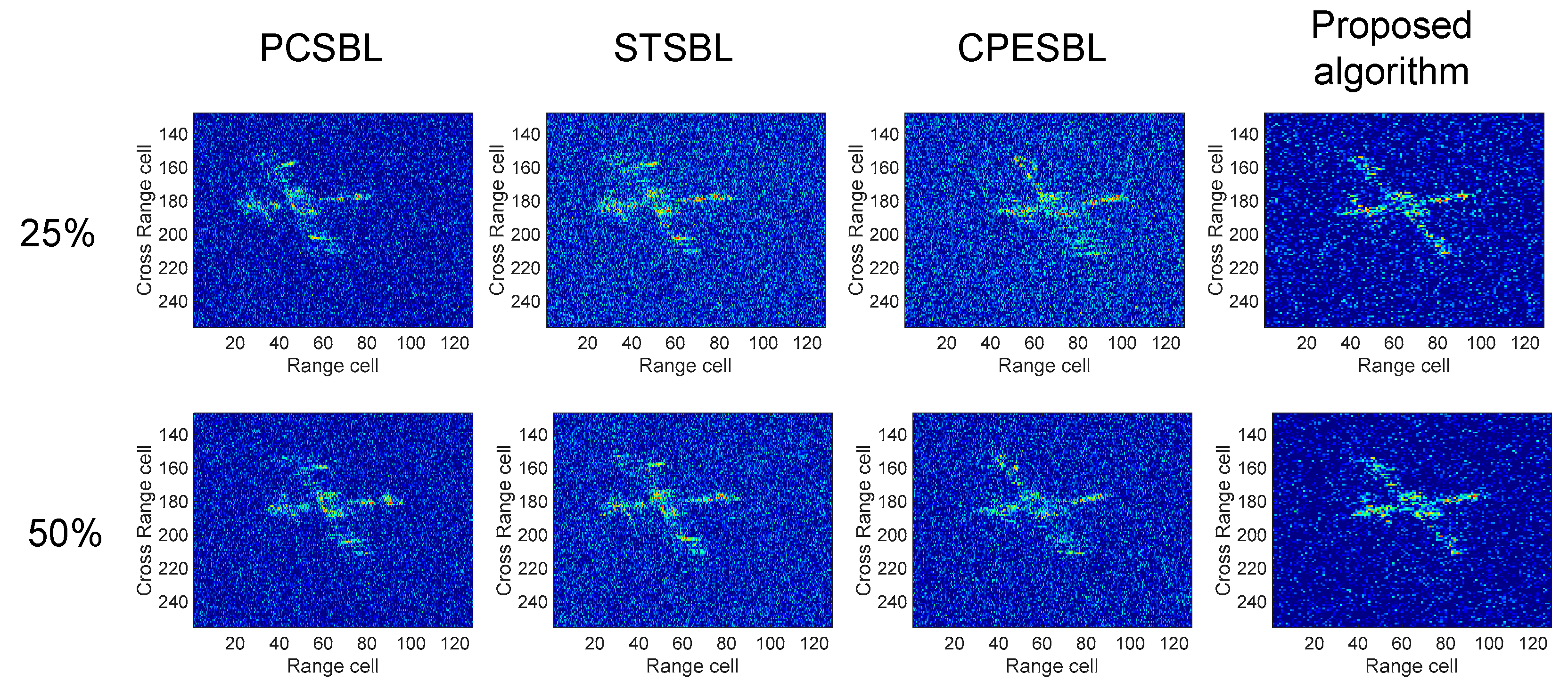
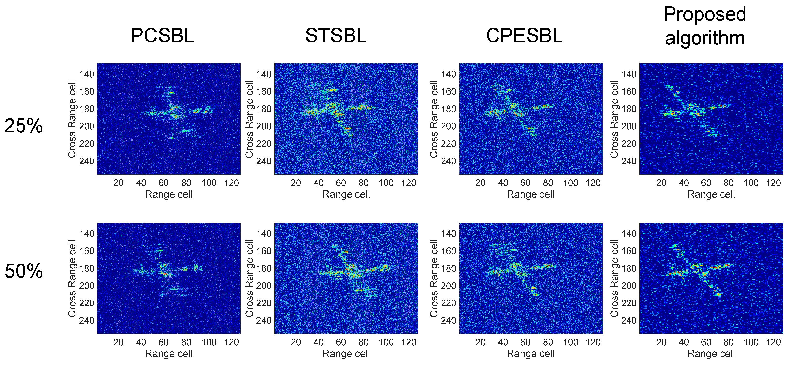
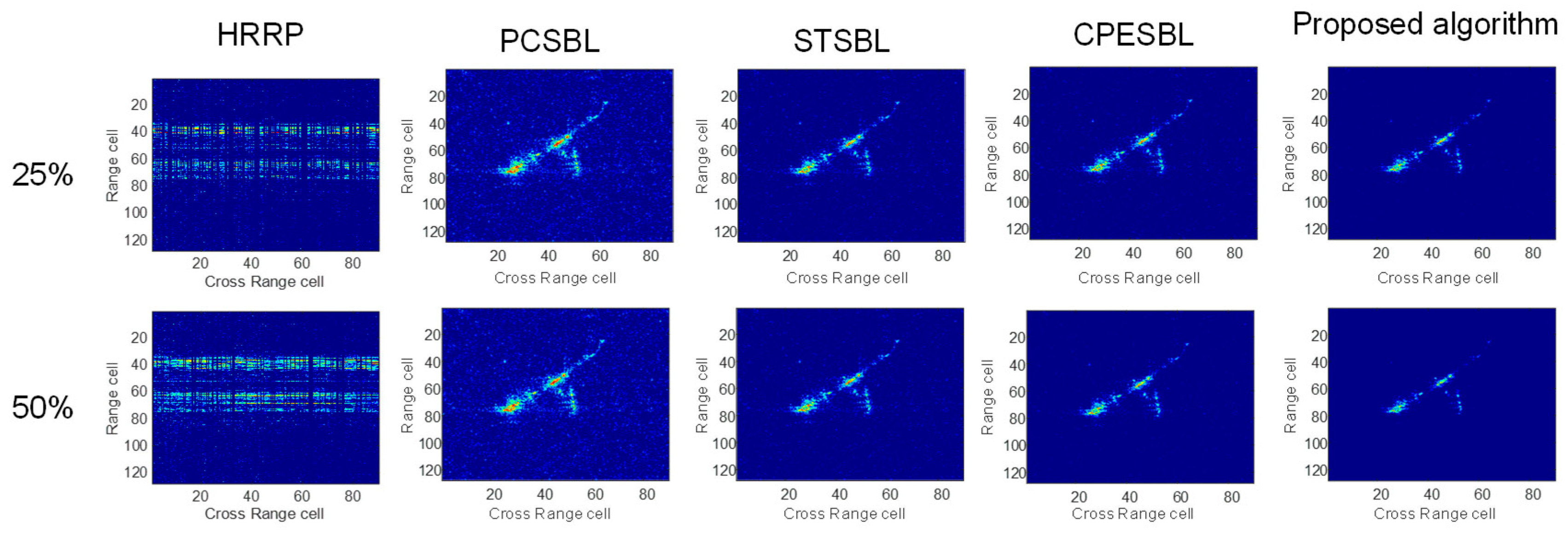
As illustrated in Figure 3, the imaging results of the target under varying sparsity levels are presented for the random sparse pattern. The first vertical column displays the HRRP imaging of the target following sparse processing. In this scenario, the loss of certain pulse data significantly compromises the imaging quality. At a sparsity level of 75%, the conventional PCSBL algorithm exhibits considerable reconstruction errors, resulting in a markedly blurred image. The STSBL algorithm, incorporating tensor structures, improves reconstruction accuracy; however, its treatment of phase information remains inadequate, leading to the omission of key scattered points, which results in localized blurring within the ISAR image. The CPESBL algorithm, which integrates phase reconstruction, yields a more refined imaging focus. The proposed HVB-MI algorithm, by introducing time-correlated coupling mechanisms, significantly enhances reconstruction precision, thereby achieving the highest imaging resolution and optimal focus. This enables an exceptionally high-resolution representation of the target’s structural features. As the sparsity level decreases, the resolution of the images generated by all three algorithms deteriorates. At a sparsity rate of 25%, the increased loss of pulse data leads to a reduction in resolution across all three algorithms. Nevertheless, the proposed HVB-MI algorithm consistently produces high-resolution imaging of the target, maintaining superior performance even under these challenging conditions.

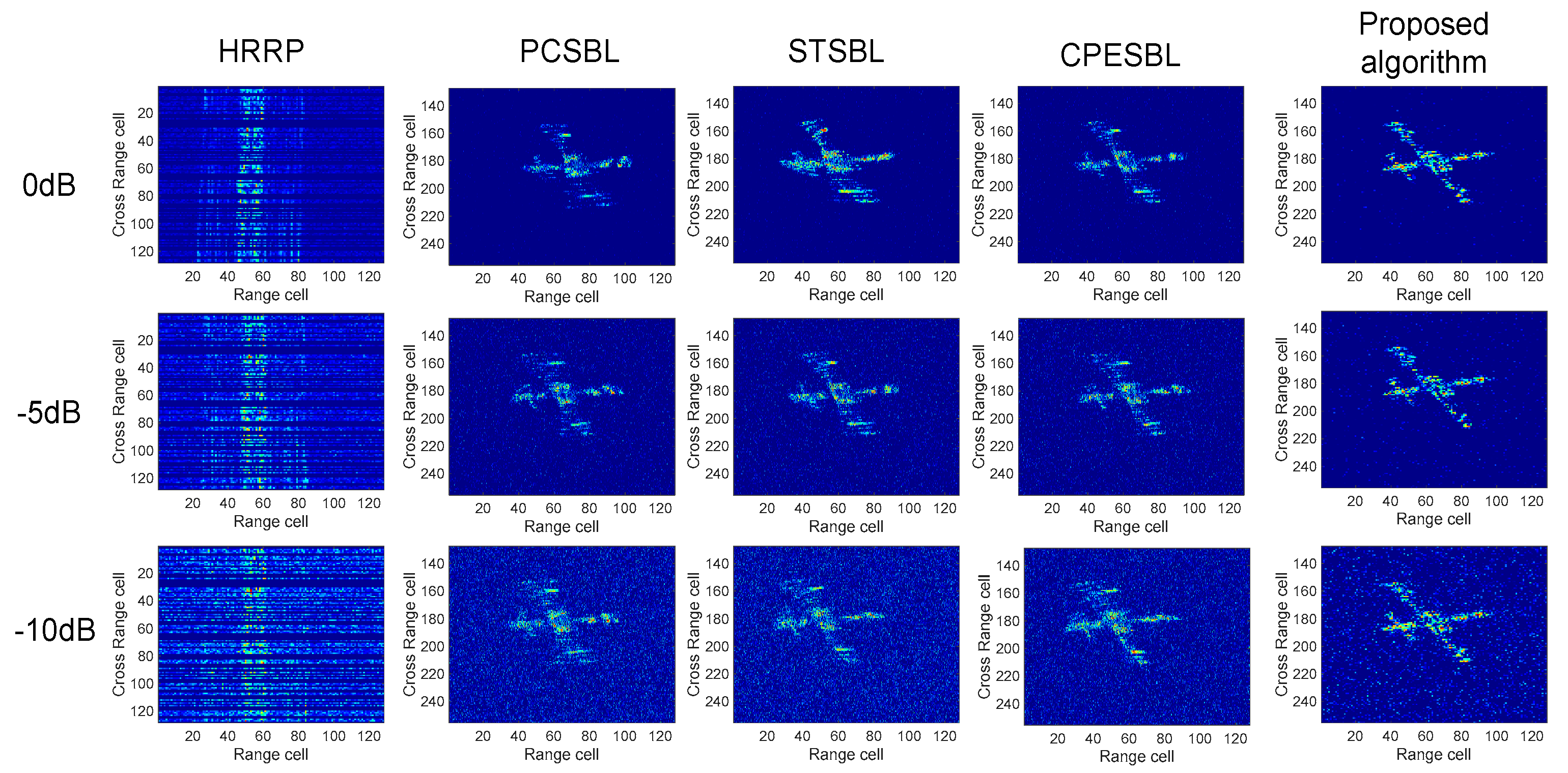
As shown in Figure 4, the ISAR imaging of the target under different sparsity levels in continuous mode is presented. It is evident that the traditional PCSBL algorithm is significantly affected, resulting in blurred regions and the loss of scattered points. The STSBL algorithm improves the resolution of target imaging but introduces some trailing effects and also suffers from scattered point omissions. The CPESBL algorithm performs better in reconstructing the main target imaging; however, some trailing artifacts remain. As the sparsity level decreases, the imaging resolution of all algorithms declines. Nevertheless, the proposed HVB-MI algorithm consistently achieves relatively clear imaging in the continuous sparse data mode.

To quantitatively analyze the imaging performance of the algorithms, Figure 5 presents the convergence curves for each algorithm under two different sparsity modes. It is evident that the proposed HVB-MI algorithm consistently achieves the fastest convergence, owing to its incorporation of time-correlated high-dimensional matrix coupling. The conventional PCSBL algorithm, due to its need to directly estimate the full-size spatial covariance matrix, experiences a rapid increase in computational complexity as the dimensionality grows, particularly when dealing with high-dimensional data. The STSBL algorithm, by leveraging tensor decomposition to reduce matrix dimensions, improves efficiency; however, it still faces limitations when processing time-correlated data matrices. The CPESBL algorithm can directly process data in the complex domain. In comparison, the proposed HVB-MI algorithm maintains superior convergence speed across different sparsity modes, outperforming the other algorithms in terms of both efficiency and robustness.

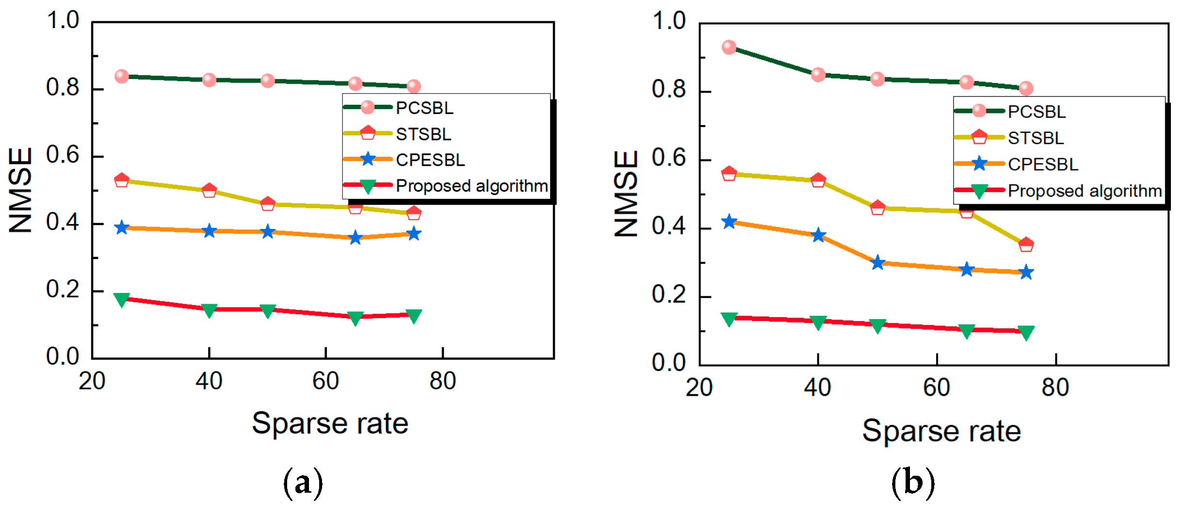
Figure 6 illustrates the variation of NMSE with respect to different sparsity rates under various sparsity modes. Each data point represents the result of 30 Monte Carlo simulations, with a maximum iteration limit set to 1000 for each algorithm. The results demonstrate that, under all sparsity modes, as the sparsity rate decreases, the NMSE increases for all algorithms. However, the proposed algorithm consistently maintains a lower NMSE, outperforming the other methods across all sparsity rates.

For comparison, we briefly summarize the per-iteration complexity of baseline methods. PCSBL requires full posterior updates with structured coupling, leading to a typical cost of $O(M^3)$. STSBL jointly models spatial and temporal correlations, involving Kronecker-structured updates with cost $O(M^2+M{N}^2)$. CPESBL incorporates enhanced coupling priors and often uses EM-based hyperparameter optimization, generally maintaining a similar complexity around $O(M^3)$. In contrast, the proposed algorithm maintains a significantly lower per-iteration cost of $O(NKM+M^2)$, while also supporting parallel updates across spatial locations, making it more scalable for large-scale high-resolution imaging.

Table 2. IC and IE of imaging results with different algorithms.

	Sparse Rate	Indicate	PCSBL [32]	STSBL [39]	CPESBL [40]	Proposed Algorithm
Random sparse mode	25%	IC	13.141	15.337	17.576	20.882
		IE	14.092	13.227	12.162	10.227
	50%	IC	14.257	15.225	18.374	20.698
		IE	13.876	12.005	11.284	10.647
	75%	IC	14.498	15.976	18.041	21.033
		IE	12.361	11.882	10.597	9.681
Continuous sparse mode	25%	IC	13.878	15.982	17.884	21.027
		IE	14.868	14.057	13.085	10.862
	50%	IC	14.387	17.259	18.959	21.224
		IE	13.661	12.784	11.939	10.072
	75%	IC	14.986	16.054	18.176	21.684
		IE	13.021	11.976	10.961	9.216

presents a quantitative comparison of the performance of various algorithms based on the imaging results. In this study, image entropy (IE) is calculated based on the method proposed in [41], and image contrast (IC) is computed according to [42]. It is evident that as the sparsity rate decreases, the IC value decreases, while the IE value increases. Nevertheless, the proposed algorithm consistently achieves higher IS values and lower IE values, demonstrating its superior performance across different sparsity conditions.

To further evaluate the clarity and structural focus of the reconstructed images under varying sampling conditions, we computed the Laplacian Variance (LV) for all competing methods. As summarized in

Table 3. LV of imaging results with different algorithms.

	Sparse Rate	Indicate	PCSBL [32]	STSBL [39]	CPESBL [40]	Proposed Algorithm
Random sparse mode	25%	LV	121.9	135.4	153.7	214.5
	50%	LV	137.8	150.1	168.9	231.2
	75%	LV	153.3	161.7	190.5	249.6
Continuous sparse mode	25%	LV	117.2	131.6	148.4	204.8
	50%	LV	131.8	146.3	159.2	221.6
	75%	LV	145.7	163.5	182.9	235.7

, the proposed algorithm consistently achieves the highest LV values across different sampling rates and in both random and continuous sampling modes, indicating superior edge sharpness and overall image focus.

At a 75% sampling rate in the continuous sparse mode, the proposed method achieves an LV of 235.7, which is substantially higher than that of PCSBL (145.7) and CPESBL (182.9), with improvements of 61.7% and 28.9% over them, respectively. These results demonstrate the effectiveness of the proposed approach in preserving fine structural details and maintaining sharp target contours.

This performance gain is primarily attributed to the method’s ability to jointly model inter-channel correlations and structured sparsity through a hierarchical variational Bayesian framework. In contrast, conventional methods typically treat receiving channels independently or lack sufficient structural regularization, making them more susceptible to noise interference and edge blurring. The proposed algorithm effectively enhances consistent target features and suppresses incoherent artifacts, resulting in sharper edges and improved focus in the final ISAR images.

Despite operating on motion-compensated data, conventional reconstruction methods such as PCSBL, STSBL, and CPESBL still suffer from residual defocusing. This is primarily due to their limited modeling capacity—e.g., ignoring inter-channel structure, oversimplified noise assumptions, or static regularization strategies. In contrast, the proposed method leverages a coupled sparse prior and a GMM-based noise model, enabling it to preserve coherent target structures and suppress background artifacts even under imperfect motion correction. These modeling advantages are particularly important in under-sampled or noisy conditions, where accurate structure recovery is challenging.

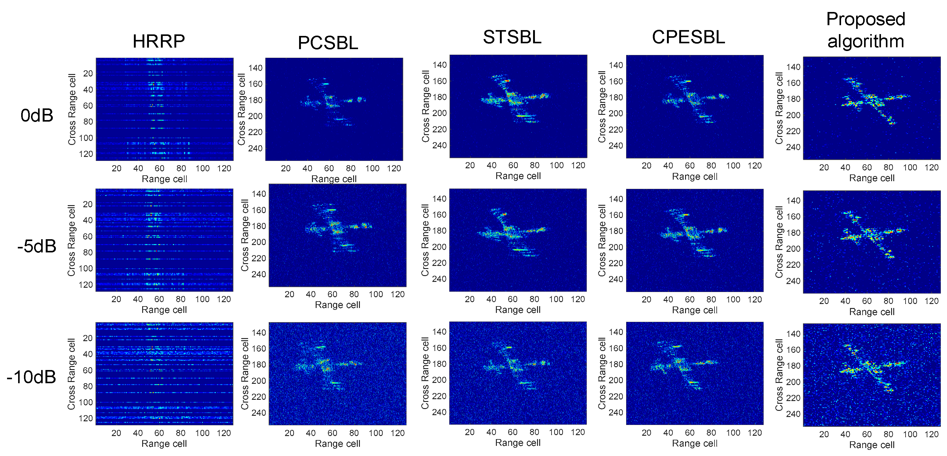
To rigorously evaluate the performance of the proposed algorithm, a comparative analysis is conducted with alternative methods under mixed noise conditions, considering a range of SNR and sparsity levels. In contrast with traditional experimental setups, the noise in this study is modeled as a mixture of Gaussian and Laplace distributions, which more closely approximates real-world noise environments and their impact on algorithm performance. The SNR values employed in the experiments are [0, −5, −10] dB. As illustrated in Figure 7, Figure 8, Figure 9 and Figure 10, the influence of mixed noise becomes increasingly significant as the SNR decreases, resulting in a gradual degradation of image clarity across all algorithms. The conventional PCSBL algorithm exhibits progressive defocusing, with a marked decline in image quality as the noise level intensifies. The STSBL algorithm, by incorporating tensor decomposition, offers partial noise suppression, yet it does not fully address the distortion of phase information, leading to minor inaccuracies in the reconstruction of scattered points, particularly under low SNR conditions, which results in the omission of critical imaging details. The CPESBL algorithm, which integrates both amplitude and phase information, effectively reduces noise; however, its performance is still somewhat constrained in highly noisy environments. The proposed HVB-MI algorithm, by incorporating an iterative optimization process tailored for mixed noise, effectively mitigates correlated noise interference. Moreover, through the coupling of time-correlated data, it preserves the structural integrity of weak scatterers and enhances the reconstruction of continuous structural features, thereby providing a more precise and reliable representation of the target’s structural characteristics.

Table 4. IC and IE of imaging results with different SNRs.

	Sparse Rate	Indicate	Algorithm	SNR
				0 dB	−5 dB	−10 dB
Random sparse mode	25%	IC	PCSBL	12.886	11.623	9.557
			STSBL	13.252	12.763	10.982
			CPESBL	15.057	14.358	13.979
			Proposed algorithm	18.743	16.228	15.820
		IE	PCSBL	15.447	16.352	18.107
			STSBL	14.572	15.212	16.033
			CPESBL	12.667	13.079	14.131
			Proposed algorithm	10.857	11.596	12.354
	50%	IC	PCSBL	14.637	13.884	12.782
			STSBL	15.271	14.081	13.572
			CPESBL	17.356	16.925	14.694
			Proposed algorithm	19.563	17.998	16.388
		IE	PCSBL	14.302	15.098.	16.872
			STSBL	13.017	14.232	15.386
			CPESBL	11.998	13.071	14.562
			Proposed algorithm	10.003	10.879	11.378
Continuous sparse mode	25%	IC	PCSBL	13.726	12.864	11.957
			STSBL	14.857	13.876	14.028
			CPESBL	15.659	15.232	14.183
			Proposed algorithm	18.995	16.857	16.029
		IE	PCSBL	15.021	16.652	17.984
			STSBL	14.257	15.621	16.865
			CPESBL	12.569	13.887	14.626
			Proposed algorithm	10.323	11.326	12.943
	50%	IC	PCSBL	14.885	13.698	12.036
			STSBL	15.527	14.953	13.687
			CPESBL	17.853	16.584	15.377
			Proposed algorithm	19.697	17.692	16.233
		IE	PCSBL	14.968	15.023	15.854
			STSBL	13.854	14.074	14.684
			CPESBL	12.663	13.282	13.481
			Proposed algorithm	10.035	10.206	10.654

provides a quantitative assessment of the imaging results for each algorithm under varying conditions. As the SNR decreases, there is a noticeable increase in the IE value, accompanied by a gradual reduction in the IS value. Across all conditions, the algorithm proposed in this work consistently outperforms the others, achieving the highest IS values and the lowest IE values. These results underscore the robustness of the algorithm, delivering superior performance at different SNRs and producing ISAR images of exceptional quality.

To further evaluate the robustness of the proposed algorithm under different noise levels, we computed the LV of reconstructed images at SNR levels of 0 dB, −5 dB, and −10 dB. As shown in

Table 5. LV of imaging results with different SNRs.

	Sparse Rate	Indicate	Algorithm	SNR
				0 dB	−5 dB	−10 dB
Random sparse mode	25%	LV	PCSBL [32]	108.9	86.7	75.4
			STSBL [39]	121.4	98.2	84.5
			CPESBL [40]	138.7	113.6	98.3
			Proposed algorithm	196.5	162.3	137.8
	50%	LV	PCSBL [32]	133.4	110.5	85.1
			STSBL [39]	145.1	121.8	94.2
			CPESBL [40]	159.3	134.2	105.3
			Proposed algorithm	213.2	188.1	153.6
Continuous sparse mode	25%	LV	PCSBL [32]	103.5	83.9	62.8
			STSBL [39]	116.7	94.1	70.2
			CPESBL [40]	133.4	108.3	82.7
			Proposed algorithm	195.8	180.5	145.2
	50%	LV	PCSBL [32]	126.8	104.9	80.5
			STSBL [39]	140.3	116.5	89.8
			CPESBL [40]	154.2	129.6	101.1
			Proposed algorithm	208.6	195.7	161.4

, the proposed method consistently achieves the highest LV values across all sampling modes and rates, even under severe noise degradation. Under the random sampling mode with a 25% sampling rate, the proposed method achieves an LV of 137.8 at −10 dB, significantly outperforming CPESBL (98.3) and STSBL (84.5), with relative improvements of 40.2% and 63.1%, respectively, demonstrating outstanding noise robustness. Similar trends are observed at higher sampling rates and under the continuous sampling mode, where the proposed approach maintains superior performance in terms of image sharpness and structural clarity.

This superior performance is primarily attributed to the algorithm’s ability to jointly model inter-channel correlations and structured sparsity through a hierarchical variational Bayesian framework. Moreover, unlike PCSBL, STSBL, and CPESBL, the proposed method adopts a GMM prior, allowing it to better capture the complex statistical distributions of ISAR targets and contributing to its superior reconstruction performance. By leveraging multi-angle coherence and a flexible prior structure, the proposed method effectively suppresses incoherent noise and enhances consistent structural features.

In contrast, traditional methods either neglect inter-channel dependencies or impose rigid, unimodal sparsity priors, limiting their adaptability to complex signal distributions and reducing their noise robustness. As a result, they tend to produce blurred contours, lower focus, and incomplete structural recovery, particularly under low-SNR or under-sampled conditions.

Figure 11 presents a visual comparison between the proposed full model and its simplified version without structural priors. As shown in Figure 11a, the absence of structural priors leads to highly fragmented features in the reconstructed image, where most scatterers are distributed as isolated points. The spatial coherence of the target is significantly degraded, with critical structures such as wings and fuselage becoming indistinct. In contrast, the full model successfully restores the overall shape of the target, exhibiting sharper contours and fewer background artifacts. This comparative analysis validates the pivotal role of structural priors in enhancing spatial consistency, suppressing non-structural noise, and improving reconstruction fidelity. The proposed multi-channel joint prior not only models inter-channel joint sparsity but also ensures simultaneous imaging of spatially correlated scatterer groups, thereby accurately reflecting the geometric structure of real-world targets.

Figure 12 and Figure 13 compare the imaging performance of PCSBL, STSBL, CPESBL, and the proposed algorithm under low signal-to-noise ratio (SNR = −15 dB) for both the random sparse mode and the continuous sparse mode. It can be observed that under such low SNR conditions, all benchmark methods exhibit varying degrees of image degradation, with increased background noise and loss of structural clarity. In the random sparse mode, PCSBL and STSBL struggle to suppress background clutter, resulting in noisy reconstructions with limited scatterer visibility. CPESBL achieves slightly better noise suppression but still fails to recover fine structures. In contrast, the proposed algorithm yields noticeably cleaner images, with enhanced target outlines and stronger suppression of incoherent noise, particularly at higher sampling ratios.

A similar trend is seen in the continuous sparse mode. While the baseline methods produce blurred or fragmented reconstructions, the proposed method retains a clearer contour and more coherent structure, even under severe noise. These results demonstrate the robustness of the proposed multi-channel Bayesian framework against noise and its advantage in preserving structural sparsity under challenging imaging scenarios.

To assess the structural fidelity across varying sampling rates,

Table 6. (a) Comparison of CORR of different algorithms (random sparse mode under SNR = −15 dB). (b) Comparison of PSNR of different algorithms (random sparse mode under SNR = −15 dB). (c) Comparison of PSNR of different algorithms (continuous sparse mode under SNR = −15 dB). (d) Comparison of CORR of different algorithms (continuous sparse mode under SNR = −15 dB).

Sampling Rate	PCSBL [32]	STSBL [39]	CPESBL [40]	Proposed
(a)
25%	0.661	0.772	0.805	0.891
50%	0.681	0.792	0.826	0.902
(b)
25%	19.4	19.8	22.3	27.1
50%	21.2	21.6	24.0	28.6
(c)
25%	18.6	19.2	21.7	26.4
50%	20.5	21.1	23.6	28.2
(d)
25%	0.652	0.766	0.783	0.882
50%	0.669	0.782	0.802	0.894

a reports the correlation coefficients (CORRs) for all five algorithms in accordance with the visual results shown in Figure 12. The proposed method achieves the highest CORR values at each sampling level—0.891 at 25% and 0.902 at 50%, demonstrating its superior capacity to preserve spatial structure under sparse observations. Compared to CPESBL, PCSBL, and STSBL, our method consistently exhibits improved structural agreement with the reference image.

The performance gap becomes more evident under lower sampling ratios, where competing methods suffer from loss of continuity and scattering ambiguity, while the proposed algorithm maintains coherent contours and fine structures. This validates the effectiveness of the multi-channel coupled inference and hierarchical modeling design.

To objectively evaluate the pixel-level fidelity of the reconstructed images, Peak Signal-to-Noise Ratio (PSNR) values under different sampling rates are reported in Table 6b. The proposed algorithm consistently achieves the highest PSNR across all settings—27.1 dB at 25% and 28.6 dB at 50%, indicating its strong capability in recovering fine spatial structures while suppressing noise and distortion.

The proposed method preserves sharper edges and more coherent target shapes than other baselines. This performance advantage arises from the hierarchical sparsity modeling, the use of multi-channel prior structures, and the application of variational Bayesian inference under a Gaussian mixture noise model. This integrated framework improves robustness under under-sampling and enhances the recovery of high-frequency details in complex imaging scenarios.

To evaluate the reconstruction quality under random sparse sampling, Table 6c,d reports the PSNR and CORR metrics for all competing methods. The proposed algorithm consistently achieves the highest performance across all sampling rates. Specifically, it yields 26.4 dB and 28.2 dB in PSNR at 25% and 50% sampling, respectively, indicating superior noise suppression and structure preservation.

In terms of structural similarity, the CORR values achieved by the proposed method are 0.882 and 0.894, outperforming all traditional algorithms. These results demonstrate the robustness of the proposed approach in preserving global target structure and fine spatial textures under highly incomplete measurements. The improvements are attributed to the integration of hierarchical priors, multi-channel modeling, and variational inference with a Gaussian mixture likelihood.

To evaluate the robustness of the proposed algorithm under realistic low-visibility conditions, additional experiments were conducted at SNRs of −10 dB and −15 dB. These settings simulate challenging environments where target returns are weak or heavily embedded in background clutter.

As shown in Figure 12 and Figure 13, even under an extremely low SNR of −15 dB, where the target signal is nearly indistinguishable from the noise floor, the proposed method successfully reconstructs a coherent and focused ISAR image. In contrast, baseline methods such as PCSBL, STSBL, and CPESBL exhibit severe degradation and defocusing effects.

This evidence highlights the strength of the proposed GMM hierarchical and coupled modeling approach, particularly in its ability to preserve structural consistency despite the presence of strong noise or interference.

While HVB-MI demonstrates robust reconstruction performance under moderate bandwidth reduction and in the presence of complex background interference, its effectiveness is fundamentally constrained by the information content available in the observations. As bandwidth decreases, both range resolution and the number of frequency-domain samples shrink, resulting in reduced observability and increased underdetermination of the imaging problem.

In particular, when multiple scatterers fall within a single resolution cell and exhibit similar Doppler signatures over time,

$${\varphi }_1(t)\approx {\varphi }_2(t)\approx \cdots \approx {\varphi }_K(t)$$

(56)

The system is unable to distinguish them spatially or temporally. In such cases, the posterior inference—regardless of algorithmic complexity—becomes limited by the Shannon capacity bound, and precise structural recovery is no longer possible. Therefore, HVB-MI is more effective in scenarios where resolution degradation is moderate and structural aliasing remains distinguishable through temporal or spectral differences. Under extreme bandwidth limitations, the goal of reconstruction should shift from resolving fine-scale structures to preserving the global consistency and interpretability of the image.

4. Real-Data Imaging Results and Analysis

In this section, we conduct a real-data experiment to verify the practical effectiveness of the proposed method. The dataset was collected using a ground-based X-band ISAR system and involves a maneuvering target under non-ideal conditions. Compared with simulations, this scenario contains more realistic phenomena, such as irregular motion-induced Doppler, clutter, and system noise.

To evaluate the effectiveness of the proposed algorithm, experiments were conducted using measured data. The measured data were collected from a B727. The corresponding radar parameters are listed in

Table 7. Radar parameters.

Parameter	Value
Carrier frequency	9 GHz
Pulse repetition interval	3.2 ms
Band width	150 MHz

. To validate the effectiveness of the proposed algorithm, four algorithms were compared and imaged, with sparsity rates of 50% and 25%, respectively.

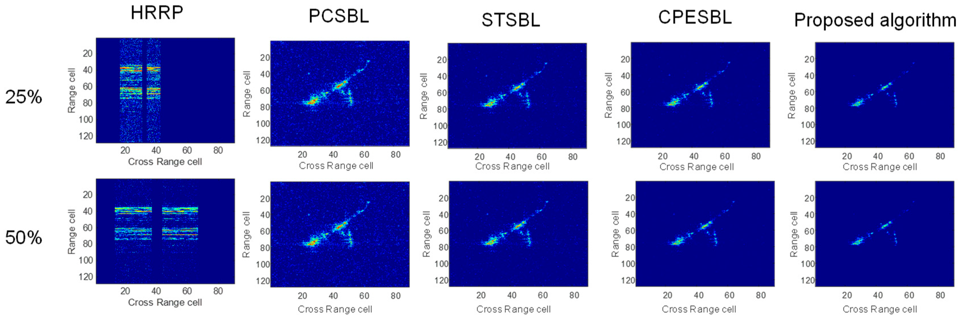
As illustrated in Figure 14 and Figure 15, the comparative visual results further validate the superior imaging performance of the proposed algorithm. While PCSBL is able to retain most of the target’s prominent features, its sensitivity to noise leads to the suppression of weak scatterers, ultimately limiting overall resolution. Although the SMSBL algorithm introduces region-based processing to enhance local reconstruction, it lacks effective noise control, which results in fragmented target representation and poor global continuity. CPESBL performs slightly better by leveraging phase information to suppress noise to some extent; however, it still fails to resolve fine structural details, with edges remaining indistinct and blurred.

In contrast, the proposed algorithm achieves both strong noise suppression and accurate detail reconstruction. This performance stems from two factors: first, it adopts a hierarchical Bayesian model that jointly exploits structured sparsity and inter-channel correlation, allowing it to distinguish signal from noise more effectively. Second, it integrates a GMM prior, which provides a flexible and data-adaptive way to model the complex statistical properties of ISAR echoes. This enables the algorithm to preserve both dominant features and weak scatterers, resulting in clearer contours, more complete shapes, and significantly improved resolution under various sparsity levels.

It is important to note that the real-measured radar data inherently includes background clutter, irregular Doppler signatures, and system-induced noise, all of which are difficult to replicate precisely in simulations. The ability of the proposed method to maintain image clarity and preserve structural details in such non-ideal conditions further confirms its effectiveness in authentic, interference-rich operational scenarios.

To evaluate imaging performance under realistic conditions, we compare IC and IE derived from real-measured ISAR data, as summarized in

Table 8. Comparison of imaging values of different algorithms.

	Sparse Rate	Indicate	PCSBL [32]	STSBL [39]	CPESBL [40]	Proposed Algorithm
Random sparse mode	25%	IC	12.814	14.953	16.325	23.663
		IE	15.135	13.867	11.207	9.575
	50%	IC	13.594	14.368	18.374	25.698
		IE	14.272	13.375	12.582	11.026
Continuous sparse mode	25%	IC	12.995	14.873	16.284	26.828
		IE	14.997	13.672	12.887	11.005
	50%	IC	13.259	15.385	17.667	25.557
		IE	14.023	13.582	12.755	10.956

. The proposed algorithm consistently achieves the highest IC values and lowest IE values, demonstrating significant improvements over existing methods. Under the random-sparse mode with a 25% sampling rate, the proposed method achieves an IC of 23.663, which is 45.0% higher than CPESBL (16.325) and 58.3% higher than STSBL (14.953).

These improvements primarily stem from the algorithm’s ability to jointly capture structured sparsity and inter-channel correlations through a hierarchical Bayesian inference model. In contrast to STSBL and CPESBL, which often assume fixed or unimodal prior distributions, the proposed method employs a Gaussian mixture model prior, enabling better adaptation to complex real-world signal structures. As a result, it produces images with sharper contrast, clearer target edges, and reduced reconstruction artifacts, even under low sampling conditions.

As illustrated in Figure 16, the computational complexity increases with the sparsity rate, resulting in a slower convergence rate for all algorithms. In contrast, the proposed algorithm demonstrates a markedly faster convergence and delivers superior imaging performance. The experimental results underscore that, when compared to the other three algorithms, the proposed method consistently generates high-resolution ISAR images with optimal focus across various conditions, effectively mitigating the issue of degraded resolution in target imaging under complex noise environments. Thus, the aforementioned experiments provide robust evidence supporting the effectiveness and exceptional performance of the proposed algorithm.

Although the proposed algorithm does not estimate motion parameters within the inference process, its performance advantages are consistently observed in both simulated and real-data experiments. This is because the method addresses critical challenges that are often overlooked by existing ISAR imaging algorithms, such as inter-channel coupling, temporal correlation, and non-Gaussian interference. Through a coupled sparse prior, robust GMM-based noise modeling, and hierarchical variational inference, the proposed framework is able to preserve fine structural details and suppress incoherent artifacts, even under sparse and noisy conditions. As a result, the method complements motion compensation by enhancing the fidelity and robustness of image reconstruction.

5. Conclusions

This paper presents a novel hybrid sparse Bayesian prior model that combines a Gaussian mixture distribution with a temporally coupled inference structure to address the challenges of strong noise interference and low computational efficiency in ISAR imaging of complex maneuvering targets under low SNR conditions. The proposed model is formulated within a variational Bayesian framework and validated using both simulation and real-world experimental data.

Experimental results, obtained from both simulated and real datasets, validate the algorithm’s effectiveness. Specifically, the method demonstrates superior robustness in preserving target structural integrity and suppressing mixed noise, even under low SNR conditions. Compared with existing algorithms, the proposed approach achieves faster convergence and higher-resolution imaging performance.

Further evaluations show that the algorithm effectively suppresses low-dimensional artifacts arising from sparse echo data while maintaining the spatial continuity of the reconstructed ISAR images. These findings confirm that the proposed approach not only enhances reconstruction quality but also improves computational efficiency.

Taken together, the results highlight the method’s strong potential for practical application, particularly in high-resolution ISAR imaging and aerospace target identification. Future research will focus on integrating multidimensional variational optimization techniques to further improve computational scalability and extend the algorithm’s applicability in real-world engineering scenarios.