Sensor-Based Yield Prediction in Durum Wheat Under Semi-Arid Conditions Using Machine Learning Across Zadoks Growth Stages

Abstract

Yield prediction in wheat cultivated under semi-arid climatic conditions is gaining increasing importance for sustainable production strategies and decision support systems. In this study, a time-series-based modeling approach was implemented using sensor-based data (SPAD, NSPAD, NDVI, INSEY, and plant height measurements collected at four different Zadoks growth stages (ZD24, ZD30, ZD31, and ZD32). Five different machine learning algorithms (Random Forest, Gradient Boosting, AdaBoost, LightGBM, and XGBoost) were tested individually for each stage, and the model performances were evaluated using statistical metrics such as R²%, RMSE t/ha, and MAE t/ha. Modeling results revealed that the ZD31 stage (first node detectable) was identified as the most successful phase for prediction accuracy, with the XGBoost model achieving the highest R²% score (81.0). In the same model, RMSE and MAE values were calculated as 0.49 and 0.37, respectively. The LightGBM model also showed remarkable performance during the ZD30 stage, achieving an R²% of 78.0, an RMSE of 0.52, and an MAE of 0.40. The SHAP (SHapley Additive exPlanations) method used to interpret feature importance revealed that the NDVI and INSEY indices contributed the most significant values to prediction accuracy for yield. This study demonstrates that phenology-sensitive yield prediction approaches offer high potential for sensor-based digital applications. Furthermore, the integration of timing, model selection, and explainability provided valuable insights for the development of advanced decision support systems.

1. Introduction

Wheat (Triticum durum Desf.) is a strategic agricultural crop for both Türkiye and the world. With global challenges such as increasing population, diminishing resources, and climate change, studies on yield prediction in wheat have become more critical than ever [1]. The Southeastern Anatolia Region of Türkiye plays a pivotal role in durum wheat production, contributing approximately 40% of the national output [2]. However, this region suffers from high fluctuations in agricultural productivity due to its arid and semi-arid climatic conditions. Therefore, the accurate and timely yield estimation of wheat is of paramount importance for both food security and sustainable agricultural policies [3].

Traditional yield prediction approaches, including statistical regression models and process-based simulations, face significant limitations such as low spatial generalizability and high data input requirements. In response, the integration of remote sensing technologies and machine learning (ML)-based approaches has gained increasing traction in recent years [4,5]. Specifically, the use of multi-source data in conjunction with ML algorithms has enhanced prediction accuracy and added a new dimension to agricultural decision support systems.

Optical-sensor-derived indicators reflecting plant growth dynamics (e.g., SPAD, NSPAD, NDVI, and INSEY) can be easily collected under field conditions and provide real-time insights into the physiological status of crops [6,7]. Spectral indices such as NDVI have been shown to correlate strongly with yield, particularly during specific Zadoks growth stages (e.g., ZD24: early tillering; ZD30: onset of stem elongation; ZD31: critical nitrogen uptake; and ZD32: late spike emergence) [8,9]. Measurements conducted at these stages can improve nitrogen use efficiency by up to 5% while achieving yield levels comparable to traditional farmer practices [10].

In recent years, the field of yield forecasting has undergone a methodological shift with the emergence of advanced ML and deep learning (DL) architectures. In addition to conventional methods such as Random Forest and SVR, models based on LSTM and CNN have demonstrated high accuracy in studies involving time-series data [11,12]. Hybrid approaches (e.g., ANN–SVR, CNN–LSTM) have shown strong performance in modeling the complex and nonlinear relationships observed across different phenological stages. Furthermore, transfer learning and domain adaptation techniques have been increasingly applied to enhance model transferability across diverse agro-ecological zones [13]. These methodological advancements are further supported by explainable artificial intelligence (XAI) tools such as SHAP, which improve the interpretability of model decisions and their integration into decision support frameworks. The growing availability of high-frequency sensor data and improved access to computational resources have made these advanced models more applicable, even for medium-scale agricultural operations.

The success of yield prediction models depends not only on the precision of sensor data but also on the selection of appropriate ML algorithms. In the literature, a wide range of models, including Decision Trees (DT), Random Forest (RF), Gradient Boosting (GB), Support Vector Regression (SVR), and Artificial Neural Networks (ANNs), have been applied under varying environmental conditions [14,15]. Additionally, explainable AI techniques such as SHAP (SHapley Additive exPlanations) offer valuable insights into the internal decision mechanisms of these models [16].

This study aims to predict wheat yield under semi-arid climatic conditions by integrating time-sensitive optical sensor data (SPAD, NSPAD, NDVI, INSEY) and plant height measurements collected at four key Zadoks growth stages (ZD24, ZD30, ZD31, ZD32). Five distinct machine learning algorithms (Random Forest, Gradient Boosting, AdaBoost, LightGBM, and XGBoost) were applied independently to each growth stage to evaluate the temporal dynamics of model performance. In addition to traditional performance metrics (R²%, RMSE, MAE), SHAP (SHapley Additive exPlanations) analysis was employed to enhance model interpretability by quantifying the relative importance of each feature in yield prediction. A key novelty of this study lies in its comprehensive, stage-wise comparison across multiple phenological windows, whereas previous research often focused on a single growth stage (e.g., ZD31 or ZD65). By incorporating multiple time points, this research provides a deeper understanding of how phenological timing affects the accuracy and reliability of yield estimation. Furthermore, the integration of SHAP analysis offers an interpretable AI approach that goes beyond performance assessment to provide actionable insights for variable contribution. This integrated and explainable machine learning framework has the potential to inform decision-making in precision agriculture, particularly in arid and semi-arid agroecosystems, by optimizing the selection of critical growth periods and predictive algorithms for yield forecasting.

2. Materials and Methods

2.1. Materials

In this study, wheat varieties (Burgos, Perre, Sarıcanak-98, and Zühre), known for their high adaptability to the Southeastern Anatolia Region, were used along with different nitrogen doses (0, 50, 100, 150, 200, and 250 t N ha⁻¹). The selection aimed to create variability in yield and quality traits.

2.1.1. Experimental Design and Meteorological Data

The field trials were carried out for two consecutive years (2022–2024) under supplementary irrigated conditions at Talat DEMİRÖREN Research Station, situated at 36°42′ N latitude and 38°58′ E longitude, at an elevation of 410 m. The station is located at the 31st km of the Sanliurfa–Akcakale road within the GAP Agricultural Research Institute Directorate in the Harran Plain, Sanliurfa province (Figure 1c). The experiment was designed as a split plot in RCBD with three replications. Varieties were assigned to the main plots, while nitrogen doses (0, 50, 100, 150, 200, and 250 t N ha⁻¹) were allocated to the sub-plots. Each plot consisted of six rows with 20 cm row spacing, covering an area of 7.2 m² (1.2 m × 6 m). Seeds were sown between November 20 and December 20 using a sowing harvester, and preventive spraying was applied against plowing and stripe rust. Nitrogen fertilizers were supplied entirely as urea (46%), along with 0.06 t P₂O₅ ha⁻¹ phosphorus fertilizer (DAP). Since nitrogen uptake and its impact on chlorophyll levels reflected in optical sensor readings typically require 4–5 weeks, all nitrogen was applied at sowing to ensure proper calibration. This fertilization approach was implemented solely for research purposes to develop a calibration equation and is not intended as a recommendation for farmers. Irrigation was performed three times during the growing season using a sprinkler system. The field was monitored regularly, and spraying was conducted to protect against wheat rust disease. Harvesting took place between June 1 and 15 using a harvester, with a 6 m² (1.2 m × 5 m) area harvested from each plot. Although Sanliurfa is part of the Southeastern Anatolia Climate Zone, it is influenced by the Mediterranean climate, characterized by hot, dry summers and mild winters. Precipitation levels and altitude gradually increase from south to north. During the experiment, meteorological data, including temperature, humidity, and rainfall, were collected from the Research Institute’s meteorological station. The recorded data covered the period from December 2022 to July 2024.

During the period from December 2022 to July 2023, the total rainfall exhibited noticeable monthly fluctuations, with the highest precipitation recorded in March. Relative humidity remained generally stable throughout the period. Maximum temperatures showed a gradual increase, reaching their peak in June. Minimum temperatures, on the other hand, fluctuated in accordance with seasonal transitions (Figure 1a, Supplementary Table S1). From December 2023 to July 2024, rainfall amounts continued to vary by month, with March again registering the highest precipitation. Relative humidity levels remained relatively constant, while maximum temperatures steadily increased, peaking in June 2024. Minimum temperatures demonstrated distinct seasonal variations during this period (Figure 1b).

2.1.2. Soil Properties of Experimental Area

To determine the initial soil properties of the experimental field, soil samples were collected each year before sowing during the 2023 and 2024 growing seasons, at a depth of 0–30 cm. Prior to the start of the study, three randomly selected soil samples were taken from various points across the field, combined into a composite sample, and analyzed in the laboratory to determine the initial soil characteristics. Before laboratory analysis, the soil samples were air-dried and sieved through a 2 mm mesh. For the determination of the physical and chemical properties of the soil, particle size distribution (clay, silt, and sand fractions) was analyzed using the Bouyoucos hydrometer method [17]. Soil pH and electrical conductivity (EC) were measured in a saturated paste extract using pH and EC meters [18]. Organic matter content was determined via the modified Walkley–Black method [19], while calcium carbonate (lime) content was quantified using the Scheibler calcimeter method [20]. Available phosphorus (P₂O₅) was analyzed using the Olsen method [21], and available potassium (K₂O) was extracted with ammonium acetate solution. Total nitrogen (N) content was determined using the Kjeldahl method, a widely accepted and reliable technique for assessing nitrogen content in agricultural soils [22]. The results of these analyses are presented in

Table 1. Soil properties of the study area.

Soil Properties	Units	2023	2024
pH		6.95	7.52
EC	dS/cm	0.89	0.92
Saturation	%	70	72
Organic Matter	%	1.29	0.8
Lime	%	26.6	32.1
Available Phosphorus	kg/da	3.04	2.95
Available Potassium	kg/da	205	213
Total Nitrogen	%	0.086	0.091

.

2.2. Methods

2.2.1. Obtaining Plant Indices (NDVI and INSEY) Using an Optical Sensor (GreenSeeker)

Optical sensors, including the handheld Green Seeker (Trimble Inc., Sunnyvale, CA, USA), and SPAD (Konica Minolta SPAD-502, Tokyo, Japan), were used to measure NDVI and chlorophyll values at four distinct plant growth stages: Zadoks 2.4 (tillering), Zadoks 3.0 (stem emergence), Zadoks 3.1 (first internode of stem emergence), and Zadoks 3.2 (second internode of stem emergence) [23]. The GreenSeeker device, used to capture NDVI values, was positioned 60 cm above the vegetation. This instrument employs light-emitting diodes (LEDs) to emit radiation and simultaneously detect reflections in the visible (VIS—650 ± 10 nm) and near-infrared (NIR—770 ± 15 nm) spectral ranges. The NDVI values obtained during these periods were divided by the number of days since planting, above a base temperature of +4.4 °C, which is the threshold for wheat growth, to calculate the INSEY (In-Season Yield Estimation) values [24,25]. The Growing Degree Days (GDD) formula is (Tmin + Tmax)/2) − 4.4 °C, where Tmin and Tmax represent the daily minimum and maximum ambient temperatures, respectively, as outlined by [24] The system operates on the principle of spectral reflectance, using measurements at various wavelengths to calculate these values [26]. INSEY was calculated by dividing the NDVI data by the number of Growing Degree Days (GDD) greater than zero, as shown in Equations (1) and (2).

NDVI = (NIR − RED)/(NIR + RED)

(1)

INSEY = NDVI/GDD(Tmin + Tmax)/2) × 4.4

(2)

where NIR: Near Infrared; RED: Red Band; GDD: Growing Degree Days; Tmax: the highest temperature of the day; Tmin: the lowest temperature of the day.

2.2.2. Chlorophyll (SPAD) Measurements

SPAD measurements were taken using a Minolta SPAD-502 (Konica Minolta., SPAD-502, Tokyo, Japan 1989), device at four different plant growth stages: Zadoks 2.4 (tillering), Zadoks 3.0 (beginning of stem emergence), Zadoks 3.1 (first internode of stem emergence), and Zadoks 3.2 (second internode of stem emergence). The readings were averaged from the last fully developed leaves on the main stems of five randomly selected plants from each plot, as well as from three separate cuttings (bottom, middle, and tip), as described by [27]. The SPAD values from the plots were normalized by dividing them by the values obtained from the same genotype plots fertilized with the highest dose, and the resulting values are expressed in relative terms. This normalization process, referred to as NSPAD, involved converting the SPAD values taken at different times into NSPAD values, calculated as a percentage of the highest SPAD value for that variety in the trial, according to the formula (Equation (3)) [28]. The NSPAD value was used for this purpose.

NSPAD (Normalized SPAD) = SPAD (parcel)/SPAD (maximum)

(3)

2.2.3. Principal Component Analysis (PCA)

To reduce the problem of multicollinearity among variables and to transform high-dimensional data into a more interpretable structure, Principal Component Analysis (PCA) was applied. PCA groups highly correlated variables together and generates components that explain the majority of the variance, thereby enabling analysis with a reduced number of newly derived variables [29]. In the PCA implementation, the number of components was determined based on eigenvalues and the proportion of explained variance, and the loading values of these components were visualized.

2.2.4. SHAP (SHapley Additive exPlanations)

To enhance model interpretability and determine the relative impact of each variable on prediction, SHAP (SHapley Additive exPlanations) analysis was conducted. SHAP explains the contribution of each feature to the model based on game theory, making the internal decision-making mechanisms of machine learning models more transparent [30]. This method allows the identification of which features the model places greater emphasis on and enables a detailed evaluation of feature contributions across different times and models. SHAP analysis is particularly well-suited for tree-based models (e.g., XGBoost, Random Forest, LightGBM) and contributes to improving the reliability of predictions. To optimize computation time, a background dataset consisting of 100 samples was used. For each model, the mean absolute SHAP values were calculated to determine the relative importance of each feature within the model. These values were then combined to form a matrix structured as features × models, which was visualized using a horizontal bar chart. The aim of this chart is to provide a comparative illustration of which features are more dominant across models and to highlight the relative importance each algorithm assigns to the sensor data.

2.3. Architecture of Algorithms

2.3.1. Algorithms

Gradient Boosting: A robust prediction model was built using a set of weak predictors (usually decision trees) with the GBDT model, which offers high accuracy and generalizability for complex datasets [31] (Equation (4)). Hyperparameter optimization was carried out using the GridSearchCV method in conjunction with 5-fold cross-validation. The parameter range tested included the following: n_estimators = 200, learning_rate = 0.1, max_depth = 6, min_samples_split = 2, and min_samples_leaf ∈ [1, 2]. The optimal parameter combination was selected based on the highest R² score achieved on the validation set. The trained model was then applied to the independent test set and evaluated using three core regression metrics: R² (coefficient of determination), RMSE (root mean square error), and MAE (mean absolute error). To visualize the model’s predictive performance, a regression plot was generated comparing actual and predicted yield values, including a linear trend line accompanied by a 95% confidence interval.

$$\widehat{y}={\sum }_{t=1}^T\eta f_t\left(x\right)$$

(4)

T: number of iterations (trees).

η: learning rate that controls the contribution of each tree.

$f_t\left(x\right)$: prediction from the $t$-th tree.

Random Forest: By combining the predictions of multiple decision trees, the Random Forest algorithm is used to train each tree independently using randomly selected data and feature subsets (Equation (5)). The results were combined by taking the average and selecting the value with the most votes [32]. Hyperparameter optimization of the models was conducted using 5-fold cross-validation via the GridSearchCV approach. The parameter ranges explored were as follows: number of trees (n_estimators) ∈ [100, 300, 500, 700], maximum tree depth (max_depth) ∈ [3, 5, 7], minimum number of samples required to split an internal node (min_samples_split) ∈ [2, 4, 6], minimum number of samples required at a leaf node (min_samples_leaf) ∈ [1, 2, 3], and number of features to consider when looking for the best split (max_features) ∈ [‘auto’, ‘sqrt’]. The optimal model was selected based on the parameter combination that achieved the highest R² value on the validation set. Once optimized, the model was trained on the training dataset and subsequently used to make yield predictions on the independent test data. The model’s performance was evaluated using three commonly employed regression metrics: coefficient of determination (R²), root mean square error (RMSE), and mean absolute error (MAE). In addition to numerical evaluation, a regression plot comparing observed and predicted yield values was generated. This plot included a linear trend line and 95% confidence interval to assess model fit visually. Furthermore, the model-derived feature importances were extracted, and the relative contribution of each sensor-based variable to yield prediction was visualized using a horizontal bar chart.

$$\widehat{y}={\displaystyle \frac{1}{T}}{\sum }_{t=1}^T{f}_t\left(x\right)$$

(5)

T: total number of trees in the forest.

$f_t\left(x\right)$: prediction from the $t$-th tree.

XG Boost: An ensemble model of decision trees is used by the potent machine learning algorithm XGBoost, which is based on the gradient boosting methodology (Equation (6)) [33]. Hyperparameter tuning of the XGBoost model was performed using the GridSearchCV method in combination with 5-fold cross-validation. The parameter ranges explored were as follows: n_estimators ∈ [100, 200], max_depth = 8, learning_rate = 0.1, subsample = 0.9, and colsample_bytree = 1. The optimal combination of hyperparameters was determined based on the model that achieved the highest R² value on the validation dataset. The XGBoost model trained with the optimal parameters was then evaluated on the independent test set. Model performance was assessed using three widely accepted regression metrics: R² (coefficient of determination), RMSE (root mean square error), and MAE (mean absolute error). In addition to the numerical evaluation, a regression plot was generated to visualize the model’s prediction accuracy, comparing observed and predicted yield values. The plot included a linear trend line along with a 95% confidence interval. Furthermore, the internal feature importance scores of the model were extracted, and the contribution of each sensor-based variable to yield prediction was illustrated using a horizontal bar chart.

$$\widehat{y}={\sum }_{m=1}^M{f}_m\left(x\right)$$

(6)

$\widehat{y}$ = Estimation value.

M = Total number of trees.

$f_m\left(x\right)$ = m: the value predicted by the decision tree.

LightGBM: is a gradient-boosting method designed for speed and accuracy. It builds trees using a histogram-based technique and grows them leaf-wise to minimize losses. To increase performance, parameters such as the learning rate, number of leaves, maximum depth, and feature percentage were adjusted accordingly (Equation (7)). The model was implemented using the LGBMRegressor class and trained with the following parameters: n_estimators = 200, learning_rate = 0.1, max_depth = 5, num_leaves = 31, and boosting_type = ‘gbdt’. Following training, the model was applied to the independent test set, and its performance was evaluated using three core regression metrics: R² (coefficient of determination), RMSE (root mean square error), and MAE (mean absolute error). To assess predictive performance, a regression plot was generated comparing the actual and predicted yield values, which included a regression line and a 95% confidence interval. Additionally, feature importance scores provided by the model were analyzed to determine the relative contribution of each variable to yield prediction.

$${\widehat{y}}_t={\widehat{y}}_{t-1}+f_t\left(x\right)$$

(7)

${\widehat{y}}_t$: The predicted value after the t-th iteration.

${\widehat{y}}_{t-1}$: The accumulated prediction from previous iterations.

$f_t\left(x\right)$: The new decision tree fitted to the negative gradient of the loss function at iteration t.

Adaboost: is used to build a robust regression model using weak predictors such as decision trees, where each new predictor is trained to correct the errors of the previous predictor (Equation (8)). Therefore, lowering the error rate enhances the model’s overall performance [34]. Hyperparameter tuning of the AdaBoost model was performed using the GridSearchCV method combined with 5-fold cross-validation (CV = 5). The parameters tested included n_estimators = 100, learning_rate = 0.1, and loss ∈ [‘linear’, ‘square’, ‘exponential’]. The optimal model was selected based on the parameter combination that yielded the highest R² score on the validation set. The AdaBoost model trained with these optimal hyperparameters was then applied to the independent test set and evaluated using three different regression metrics: R² (coefficient of determination), RMSE (root mean square error), and MAE (mean absolute error). To visualize the model’s predictive performance, a regression plot was created comparing the actual and predicted yield values. This plot included a linear trend line and a 95% confidence interval to better illustrate the accuracy and reliability of the model.

$$F_m\left(x\right)=F_{m-1}\left(x\right)+{\alpha }_m{h}_m\left(x\right)$$

(8)

$F_m\left(x\right)$: current model.

${\alpha }_m$: weight assigned to the m-th weak learner.

$h_m\left(x\right):$ Prediction of the $m$-th weak learner.

2.3.2. Data Preprocessing and Exploratory Data Analysis (EDA)

The dataset used in this study consisted of five independent variables derived from optical sensor measurements (SPAD, NSPAD, NDVI, INSEY) and plant height (cm), with grain yield (yield) as the target variable. These measurements were collected across four Zadoks growth stages: ZD24 (early stage), ZD30 (early mid stage), ZD31 (critical period for nitrogen uptake), and ZD32 (late stage). Since all features in the dataset were numerical, no categorical encoding was required. During the data preprocessing stage, missing values (NaNs) were detected, but their proportion was relatively low. Therefore, a simple imputation strategy was applied by replacing missing entries with the mean of each respective variable. Additionally, potential outliers in the dataset were examined using the interquartile range (IQR) method to assess data distribution and minimize distortion in model training. This preparation ensured that the dataset was both clean and consistent, enabling the reliable training of machine learning models in the subsequent analysis. In order to prevent variables with different scales from biasing the models, all independent variables were standardized using StandardScaler (with a mean of 0 and a standard deviation of 1). Before proceeding to the modeling process, the data was divided into three subsets: training (70%), validation (15%), and testing (15%). A correlation heatmap was generated to examine the relationships between the target variable (e.g., Yield) and the independent variables and to guide the selection of variables to be included in the model. This visual analysis revealed the strength and direction of the associations between variables and also provided insights into potential multicollinearity among predictors. Following the data preprocessing stage, the performance of various machine learning models was evaluated using regression plots that illustrate the relationship between actual and predicted yield values. Model performance was assessed using statistical metrics such as R², RMSE, and MAE, and these metrics were analyzed separately for each Zadoks growth stage (ZD24, ZD30, ZD31, ZD32). In addition, SHAP (SHapley Additive exPlanations) analysis was conducted for each model to determine the relative importance of features in yield prediction and to provide interpretability into the internal decision-making processes of the models. To enhance model robustness and generalizability, 5-fold cross-validation was implemented, and hyperparameters were fine-tuned using GridSearchCV optimization. ‘random_state = 42’ was used to ensure consistency in the data splitting, model training, and resampling steps. A wide range of hyperparameter values was defined for each model, and different combinations were evaluated through cross-validation. Moreover, 95% confidence intervals were estimated using the bootstrapping method, thereby improving the reliability and accuracy of the models (

Table 2. Summary of Hyperparameter tuning.

Dataset	Model	Hyperparameter	Optimal Value	Optimization	Performance Metrics
%70 Training %15 Testing %15 Validation	Random Forest	Number of Estimators	100, 300, 500, 700	5-fold cross validation GridSearchCV 95% CI	R2 RMSE MAE
		Max Depth	3, 5, 7
		Min Samples per Leaf	1, 2, 3
		min_samples_split	2, 4, 6
		max_features	‘auto’, ‘sqrt’
	Gradient Boosting	Number of Estimators	200
		Max Depth	6
		Learning Rate	0.1
		min_samples_split	2
		min_samples_leaf	1,2
	AdaBoost	Number of Estimators	100
		Learning Rate	0.1
		Loss Function	‘linear’, ‘square’, ‘exponential
	LightGBM	Boosting Type	gbdt
		Number of Estimators	200
		Learning Rate	0.1
		Max Depth	5
		num_leaves	31
	XGBoost	Number of Estimators	100, 200
		Learning Rate	0.1
		Max Depth	8
		subsample	0.9
		colsample_bytree	1

).

2.3.3. Data Analysis

The machine learning algorithms were coded in Python using Google Colab Notebook. The coding was performed using a computer (HP Victus, HP Inc., Palo Alto, CA, USA) equipped with a 13th-generation Intel Core i7 processor, 32 GB RAM, and an NVIDIA GeForce RTX 4060 graphics chip (NVIDIA Corporation, Santa Clara, CA, USA).The dataset was uploaded as a csv file to Google Colab Notebook, and the coding process started. The regression algorithms and SHAP analyses for the dataset were implemented using the Python 3 Google Compute Engine programming language. In Python, Numpy was used for numerical calculations, Pandas for data analysis, Scikit-Learn [35] for machine algorithms, and Matplotlib and Seaborn libraries for data visualization. The methodology of the machine learning approaches, including both regression modeling and SHAP-based interpretability, is detailed in the following sections. The detailed flowchart related to the research is provided below (Figure 2).

2.3.4. Performance Evaluation Metrics

Regression performance was determined by R², Mean Absolute Error (MAE), and Root Mean Squared Error (RMSE) metrics. The methodology of model evaluation metrics was detailed below (

Table 3. Performance evaluation metrics.

Metrics	Explanations	Formulations
R2	Ranges from 0 to 1, with values closer to 1 indicating that the model explains a larger proportion of the variance in the data [36,37].	${\mathrm{R}}^2=1-{\displaystyle \frac{{\sum }_{\mathrm{i}=1}^{\mathrm{n}}{\left({\mathrm{Y}}_{\mathrm{i}}-{\widehat{\mathrm{Y}}}_{\mathrm{i}}\right)}^2}{{\sum }_{\mathrm{i}=1}^{\mathrm{n}}{\left({\mathrm{Y}}_{\mathrm{i}}-\overline{{\mathrm{Y}}_{\mathrm{i}}}\right)}^2}}$
RMSE	A sensitive indicator for measuring the magnitude of forecast errors, was calculated as the square root of the mean square of the squares of the forecast errors [38].	$\mathrm{R}\mathrm{M}\mathrm{S}\mathrm{E}=\sqrt{{\displaystyle \frac{1}{\mathrm{n}}}{\displaystyle \sum _{\mathrm{i}=1}^{\mathrm{n}}}{\left({\mathrm{y}}_{\mathrm{i}}-{\widehat{\mathrm{y}}}_{\mathrm{i}}\right)}^2}$
MAE	A commonly used metric for evaluating the accuracy of regression models [39].	$\mathrm{M}\mathrm{A}\mathrm{E}={\displaystyle \frac{1}{n}}{\displaystyle \sum _{i=1}^n}\left|y_i-\widehat{y}i\right|$

).

3. Results

The yield prediction performances of various machine learning algorithms (Random Forest, AdaBoost, Gradient Boosting, LightGBM, and XGBoost), developed using sensor data (SPAD, NSPAD, INSEY, NDVI, and PH) collected at different Zadoks growth stages (ZD24, ZD30, ZD31, and ZD32), are presented in detail. The performance of the models was evaluated using specific error metrics (R², RMSE, and MAE), and the predictive power for each growth stage was compared both graphically and numerically. Furthermore, through SHAP analyses, the relative importance levels of features on yield prediction were revealed, allowing for the interpretation of the internal decision structures of the models.

According to the Pearson correlation analysis conducted in this study, statistically significant and strong positive relationships were mostly observed between yield and the indices SPAD, NSPAD, NDVI, and INSEY. Particularly during the ZD30 and ZD31 stages, high correlation coefficients were identified for SPAD (r > 0.80), NSPAD (r > 0.75), and INSEY (r > 0.85), indicating that these growth stages are physiologically critical for yield prediction. NDVI values also showed significant positive correlations with yield across all stages, with especially notable associations during ZD30 and ZD31 (r > 0.70). In contrast, plant height (PH) exhibited relatively weaker correlations with yield compared to other sensor-based indicators and even showed negative correlations in some stages. This suggests that plant height is a limited predictor for yield estimation, while spectroscopic indices, particularly INSEY and NDVI, offer more reliable insights. Overall, the ZD30 and ZD31 stages were identified as having the highest correlation values with yield prediction (Figure 3).

In the PCA analysis conducted according to Zadoks growth stages, the first two principal components (PC1 and PC2) explained 45.22% and 22.20% of the total variance, respectively, accounting for a strong cumulative variance explanation of 67.42%. The resulting biplot clearly demonstrated a distinct separation of observations across different phenological stages (ZD24, ZD30, ZD31, and ZD32) based on their spectral and physiological characteristics. Observations from ZD31 and ZD32 were more densely clustered, indicating that these stages represent critical phases of increased physiological stability in wheat plants. The analysis of vector orientations and lengths revealed that the yield, SPAD, and INSEY variables made strong positive contributions along the PC1 axis. This highlights these three variables as dominant factors influencing yield throughout the growth stages. Conversely, plant height (PH) exhibited a more pronounced effect along the PC2 axis (Figure 4a).

The PCA loading heatmap provided further insight into the dimensionality reduction process by visualizing the contributions of each variable to the first six principal components. Yield (0.49), SPAD (0.43), and PH (0.60) contributed most positively to PC1, while PH also showed the highest loading on PC2 (0.75). The NDVI and INSEY indices loaded significantly on PC3 and PC4, respectively, helping to balance the distribution of variance across other dimensions. Notably, SPAD had a negative loading on PC2 (−0.63), indicating an inverse influence in certain components, while PH showed positive loadings on both PC1 and PC2, suggesting a multifaceted influence. These findings indicate that the variance is not confined to a single axis but is distributed across a multi-dimensional structure, thereby providing a robust foundation for multivariate regression and machine learning applications (Figure 4b).

3.1. Yield Prediction by ZD Stages Using Machine Learning Algorithms

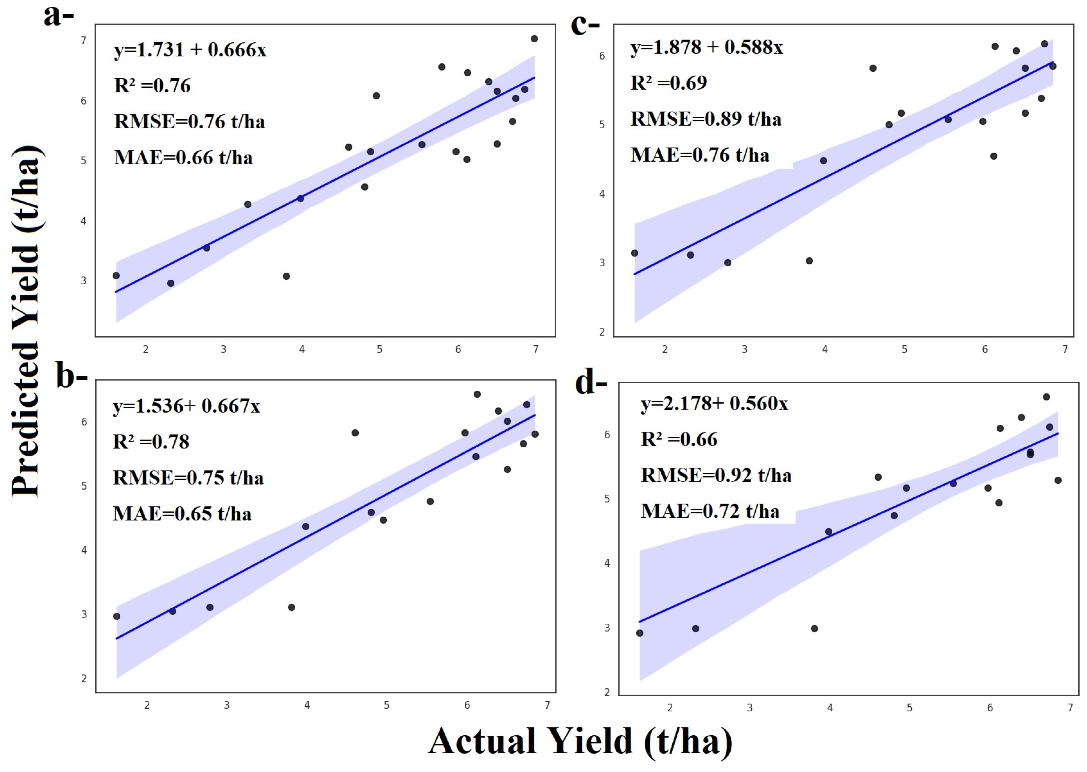
3.1.1. Random Forest and ZD Stages

According to the yield prediction results obtained using the Random Forest algorithm, the values recorded during the ZD24 stage (R² = 0.70, RMSE = 0.85 t/ha, MAE = 0.73 t/ha) indicate that spectral and physiological data collected in this early phase provide meaningful and consistent predictive power for yield (Figure 5a). A positive linear relationship was observed between the actual and predicted yield values, demonstrating that the model can perform well even during early phenological stages. Similarly, the modeling results for the ZD30 stage showed strong predictive performance with R² = 0.70, RMSE = 0.88 t/ha, and MAE = 0.68 t/ha (Figure 5b). This period represents a critical phase where nitrogen response in plants becomes more pronounced. Notably, the low MAE value suggests model stability and resilience to error, emphasizing the importance of ZD30 in yield prediction.

Among all stages, ZD31 demonstrated the highest prediction accuracy, with R² = 0.76, RMSE = 0.78 t/ha, and MAE = 0.68 t/ha (Figure 5c). These values indicate that ZD31 is the optimal time window for yield estimation, and the Random Forest algorithm effectively captured the underlying data patterns at this stage. In contrast, model performance declined markedly during ZD32, with a lower explanatory power (R² = 0.56, RMSE = 1.03 t/ha, MAE = 0.83 t/ha) (Figure 5d). This reduction likely reflects increased environmental and genetic variability in the later stages of plant development, which introduces more complex and dispersed influences on yield. The model’s lower accuracy during ZD32 confirms that earlier stages yield more reliable predictions. Overall, the findings clearly indicate that ZD31 is the most suitable phenological stage for yield prediction using the Random Forest algorithm. Moreover, spectral and physiological data collected during ZD30 and ZD31 contributed significantly to optimizing model performance.

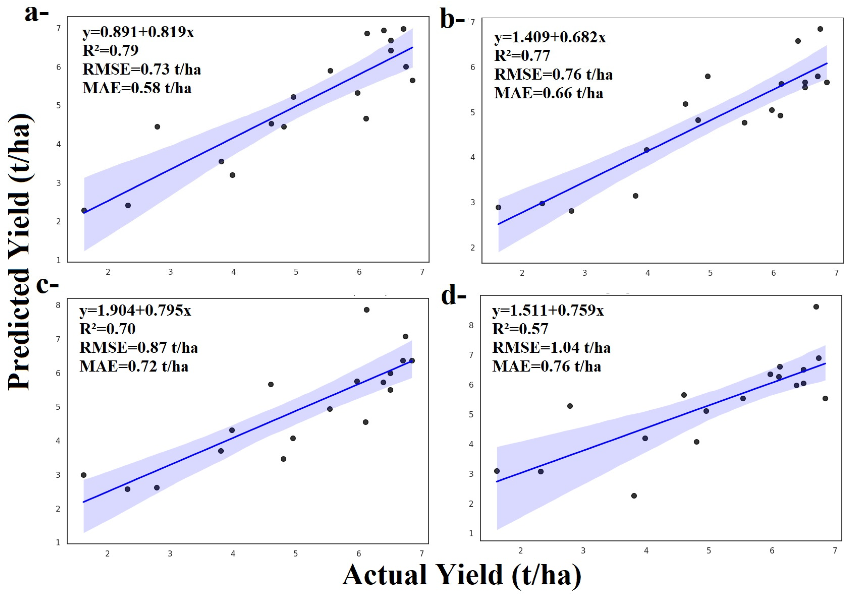
3.1.2. Adaboost and ZD Stages

The AdaBoost algorithm demonstrated a notably successful prediction performance during the ZD24 growth stage. The results R² = 0.76, RMSE = 0.76 t/ha, and MAE = 0.66 t/ha indicate that strong yield forecasts can be made even in the early developmental stages (Figure 6a). A clear linear relationship was observed between actual and predicted yield values, reflecting the model’s low-bias performance. The low error metrics confirm the high potential of sensor data for early-stage yield estimation. In the ZD30 stage, the predictive performance slightly declined. The model yielded R² = 0.69, RMSE = 0.89 t/ha, and MAE = 0.76 t/ha, suggesting that although the model continued to predict yield meaningfully, the error rates increased (Figure 6b). This may indicate that plant responses became more heterogeneous or that environmental variability influenced the model during this stage. The ZD31 stage exhibited the highest prediction performance using the AdaBoost algorithm. With values of R² = 0.78, RMSE = 0.75 t/ha, and MAE = 0.65 t/ha, the predicted yields closely matched the actual measurements (Figure 6c). As this stage represents a period of maximum nitrogen uptake and photosynthetic activity in the plant, measurements taken during this phase appear to be highly informative for the model’s learning process.

In the later stage of ZD32, the model’s explanatory power diminished, and error metrics increased. Results of R² = 0.66, RMSE = 0.92 t/ha, and MAE = 0.72 t/ha suggest that as influencing factors on yield become more complex, model performance is relatively reduced (Figure 6d). This outcome points to the potential for increased external variability and measurement errors in the late phenological stages. Overall, the AdaBoost algorithm showed satisfactory performance across all Zadoks stages, with the most successful results observed during ZD31 and ZD24. These findings emphasize the importance of intensifying sensor-based monitoring applications during these critical periods.

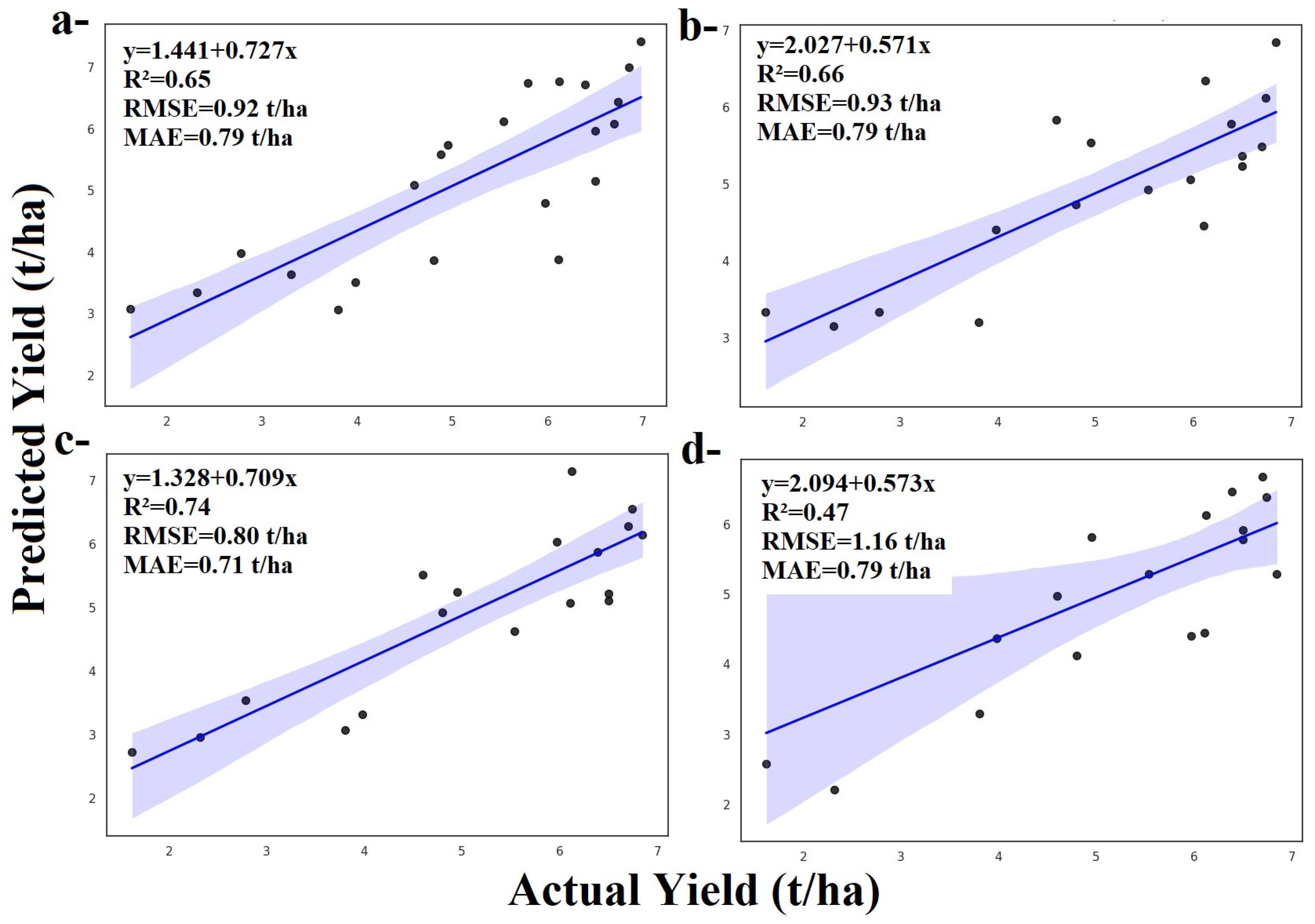
3.1.3. Gradient Boosting and ZD Stages

The Gradient Boosting model demonstrated strong performance in yield prediction during the early phenological stage ZD24. The results R² = 0.79, RMSE = 0.73 t/ha, and MAE = 0.58 t/ha indicate that the spectral and physiological data collected at this stage hold high predictive power for yield estimation (Figure 7a). The particularly low error values suggest that this growth phase provided a highly informative dataset for model training. During the ZD30 stage, the model also maintained a high level of performance, with R² = 0.77, RMSE = 0.76 t/ha, and MAE = 0.66 t/ha (Figure 7b). This stage corresponds to a phase in which the nitrogen response becomes more evident in the plant, and the high predictive accuracy reflects the model’s ability to effectively capture relevant biophysical signals.

In ZD31, a relative decrease in model performance was observed. Although the prediction strength remained acceptable (R² = 0.70, RMSE = 0.87 t/ha, MAE = 0.72 t/ha), the increase in error metrics suggests that the complexity of yield-related traits during this period may have posed limitations on the model’s learning capacity (Figure 7c). In the late developmental stage ZD32, prediction performance significantly declined. The results R² = 0.57, RMSE = 1.04 t/ha, and MAE = 0.76 t/ha suggest that data from this phenological phase are less determinative for yield prediction (Figure 7d). The drop in explanatory power during this period points to increasing environmental variability and the growing influence of non-yield factors. Overall, Gradient Boosting stood out for its high prediction accuracy and low error values, particularly during the early stages (ZD24 and ZD30). Owing to its ability to capture complex and nonlinear patterns within the data, this algorithm offers reliable predictions during specific developmental stages. However, the decline in performance in later stages underscores the importance of carefully selecting the optimal timing for model application.

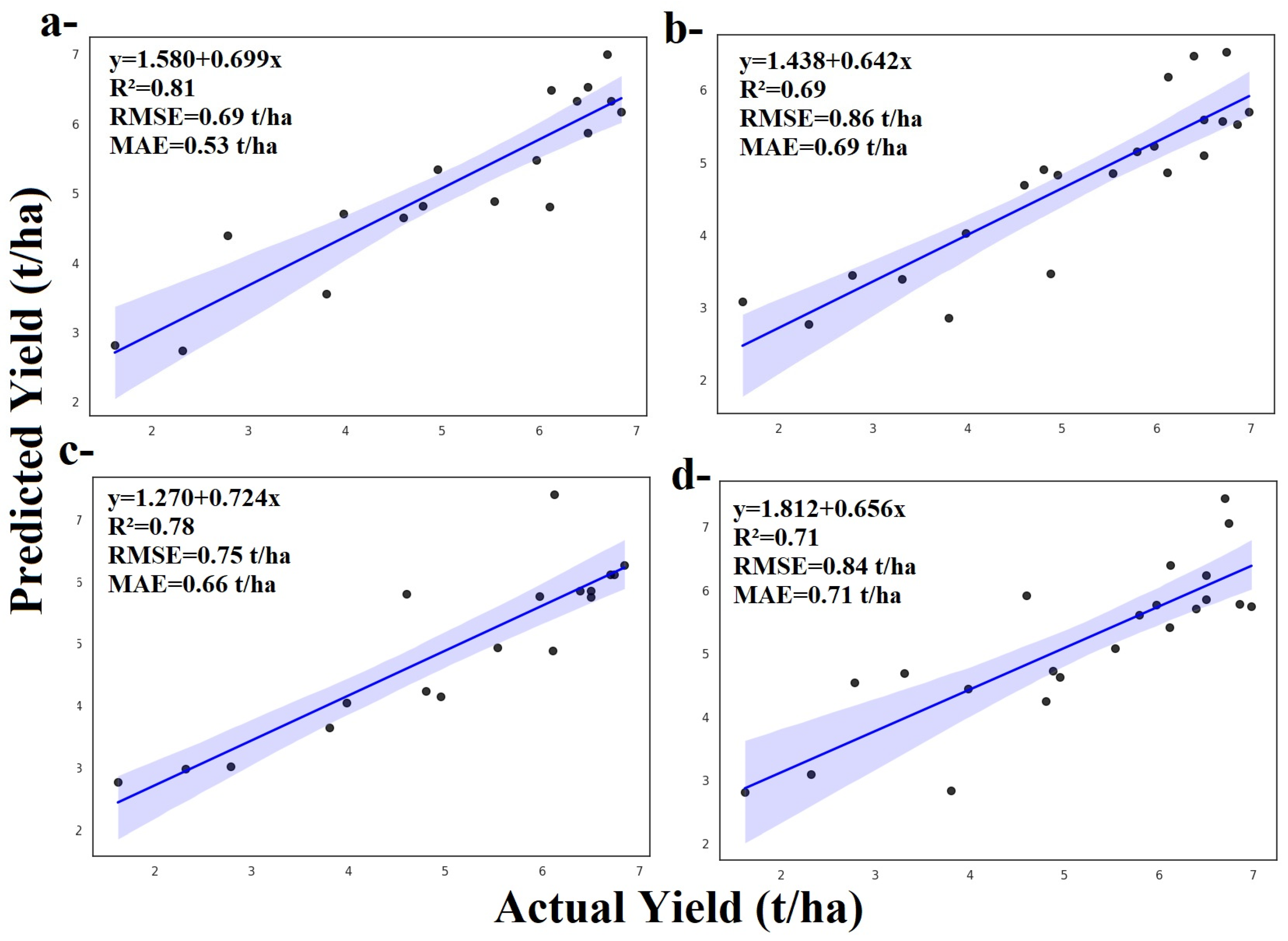
3.1.4. LightGBM and ZD Stages

In the ZD24 stage, the LightGBM algorithm exhibited a moderate level of prediction accuracy. The values obtained R² = 0.65, RMSE = 0.92 t/ha, and MAE = 0.79 t/ha indicate that while the model was able to provide a certain degree of yield prediction during the early growth phase, the error rates were relatively high (Figure 8a). This suggests that the variance in the data during this stage may be limited or that LightGBM struggled to learn the complex patterns present at this early development phase. During the ZD30 stage, the model’s performance remained at a similar level, with R² = 0.66, RMSE = 0.93 t/ha, and MAE = 0.79 t/ha (Figure 8b). Although LightGBM maintained its predictive capability during this mid-development stage, the prediction errors were not significantly reduced. This may imply that the model could not efficiently process the variance associated with spectral and physiological data during this stage.

ZD31 emerged as the most successful stage for the LightGBM algorithm. The model achieved R² = 0.74, RMSE = 0.80 t/ha, and MAE = 0.71 t/ha, demonstrating a strong alignment between predicted and actual yield values (Figure 8c). This success can be attributed to the more predictable nature of the data during ZD31 and the model’s ability to effectively learn from those structural characteristics. In contrast, the ZD32 stage showed a marked decline in model performance, with explanatory power dropping and error rates increasing (R² = 0.47, RMSE = 1.16 t/ha, MAE = 0.79 t/ha) (Figure 8d). These values suggest that LightGBM had difficulty capturing the complex data patterns of the late phenological phase, and that the physiological variability during this period negatively affected prediction accuracy. Overall, while the LightGBM algorithm demonstrated satisfactory yield prediction accuracy during ZD31, it experienced noticeable performance losses in both early (ZD24) and late (ZD32) growth stages.

3.1.5. XGBoost and ZD Stages

The XGBoost algorithm demonstrated remarkably high performance during the ZD24 stage, achieving an R² of 0.81, an RMSE of 0.69 t/ha, and an MAE of 0.53 t/ha. These results indicate that even in the early phenological stage, the model was capable of generating strong yield predictions (Figure 9a). This finding emphasizes that early-stage sensor data can provide high predictive power when processed with advanced ensemble algorithms like XGBoost. During the ZD30 stage, the model’s performance slightly declined but remained acceptable, with R² = 0.69, RMSE = 0.86 t/ha, and MAE = 0.69 t/ha (Figure 9b). These metrics suggest that although the model could capture the variability in this middle stage of development, prediction accuracy was somewhat reduced due to increasing physiological complexity.

In the ZD31 stage, the model performance improved again, yielding R² = 0.78, RMSE = 0.75 t/ha, and MAE = 0.66 t/ha (Figure 9c). This phase represents a point at which plant growth becomes more defined, and both nitrogen uptake and photosynthetic activity reach peak levels, allowing the model to perform robustly. XGBoost effectively captured the variance in this stage, indicating strong learning capacity. In the ZD32 stage, the model continued to perform satisfactorily, with R² = 0.71, RMSE = 0.84, and MAE = 0.71 (Figure 9d). These values show that while late-stage measurements still contribute to yield prediction, their effect is less prominent than during ZD31. Nevertheless, the model successfully handled the increased biophysical complexity of this phenological stage. Overall, XGBoost emerged as one of the most successful algorithms across all Zadoks stages, consistently delivering high accuracy and low error metrics. The strong statistical outcomes, observed particularly in ZD24 and ZD31, affirm the model’s effectiveness in both the early and optimal developmental phases. These findings highlight XGBoost’s capacity to learn complex inter-variable relationships and minimize errors, positioning it as a robust candidate for integration into agricultural decision support systems.

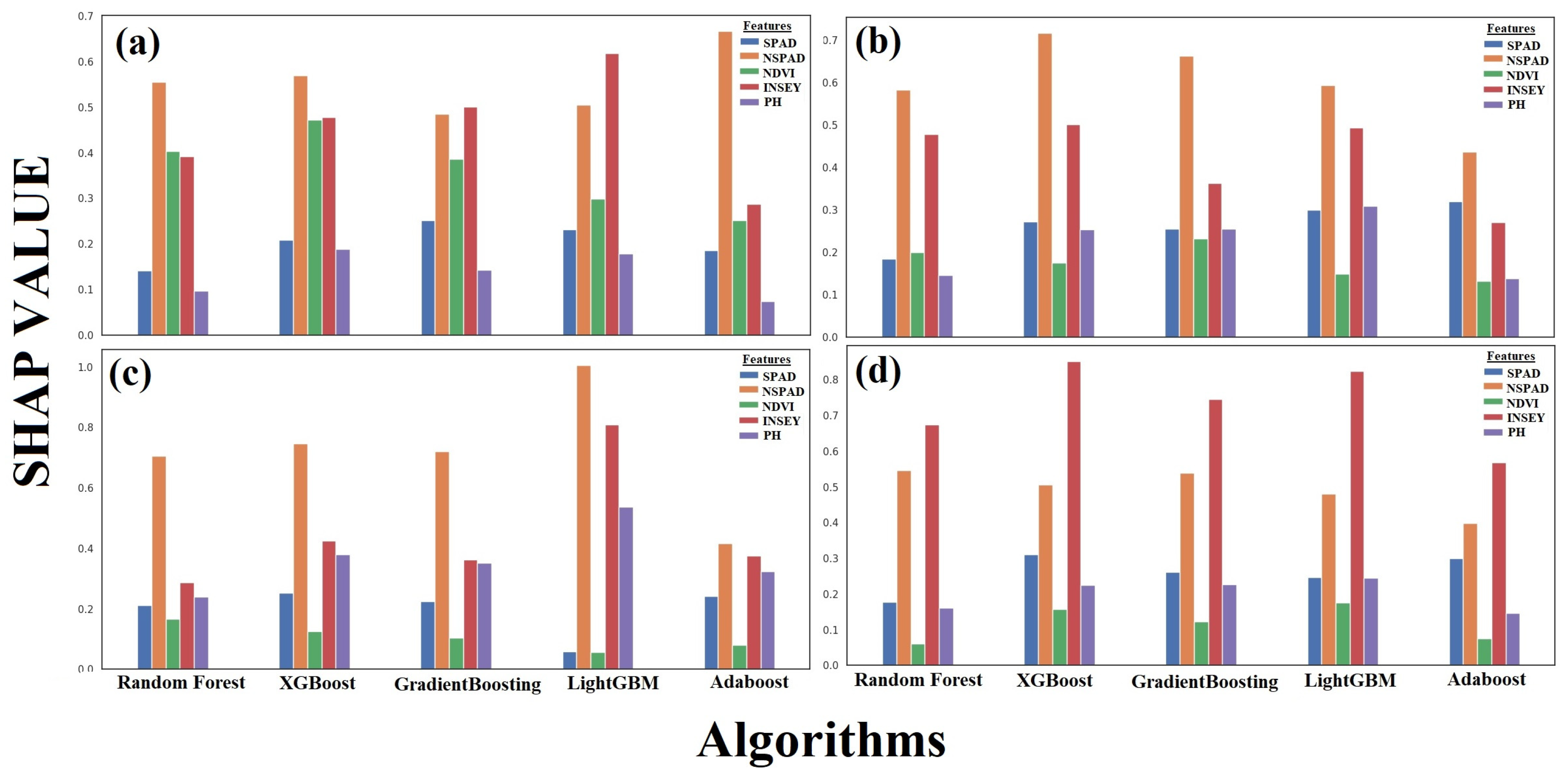
3.1.6. SHAP Analysis Interpretation Across ZD Stages

In the SHAP analyses for the ZD24 stage, NSPAD emerged as the most influential variable for yield prediction (Figure 9a). In all models, the SHAP value of NSPAD exceeded 0.5, indicating its dominant role in feature contribution. INSEY and NDVI also showed high impact, particularly in the Gradient Boosting and AdaBoost models, revealing that spectral indices exert a strong influence on yield during the early growth stage. On the other hand, plant height (PH) had the lowest SHAP values across all algorithms, suggesting its limited role in yield determination at this stage. These findings highlight the importance of variables that reflect photosynthetic activity and nitrogen status during the ZD24 phase (Figure 10a). In the ZD30 stage, NSPAD once again stood out as the most dominant feature; in the XGBoost model, its SHAP value reached as high as 0.9 (Figure 10b). This indicates that nitrogen distribution in leaves and photosynthetic efficiency have a direct impact on yield at this stage. The PH variable showed relatively higher contributions in the Random Forest and LightGBM algorithms, suggesting that structural plant parameters become more meaningful during the intermediate stage. NDVI, however, lost its importance, with very low SHAP values observed.

In ZD31, SHAP analyses revealed a joint dominance of NSPAD and INSEY across models (Figure 10c). In the XGBoost and Gradient Boosting models, the SHAP value for NSPAD reached 0.7, while INSEY showed strong contributions, particularly in AdaBoost. NDVI and PH had lower impacts during this phase, indicating that nitrogen-related parameters had a more pronounced role compared to spectral reflectance indices. These results support why ZD31 yielded the best model performances; it represents the stage where nitrogen status and spectral radiation responses align most effectively for yield prediction. During the ZD32 stage, INSEY became the most decisive variable across all models, with SHAP values exceeding 0.8 in AdaBoost and LightGBM (Figure 10d). This suggests that in the late growth stage, photosynthetic indices and light use efficiency become the dominant predictors of yield. The influence of NSPAD weakened considerably, while NDVI and SPAD contributed moderately. PH again provided limited predictive power. Overall, as nitrogen-related signals decline in later stages, spectral reflectance indices, particularly INSEY, become the primary predictive inputs (Figure 8d). These SHAP analyses demonstrate that feature importance shifts with phenological development, underscoring the critical role of time-sensitive variable weighting in yield prediction. While NSPAD was the key predictor during early and mid-growth stages, INSEY dominated the later stages. NDVI, in general, offered lower predictive strength compared to other spectral indices.

3.2. Comparision of Algorithms and ZD Periods

3.2.1. Model Performances

Overall, XGBoost emerged as the most successful model, consistently delivering the highest R² values (notably 0.81 in ZD24) and the lowest MAE and RMSE values across all Zadoks stages. Gradient Boosting and AdaBoost also demonstrated strong predictive performance, especially in ZD24 and ZD31, closely following XGBoost. Random Forest produced satisfactory results up to ZD31 but experienced a notable decline in accuracy in the ZD32 stage. LightGBM, on the other hand, showed the weakest performance, particularly during the late growth stage (ZD32), with low R² and high error metrics.

3.2.2. Zadoks Stage-Specific Observations

The ZD31 stage proved to be the most optimal for yield prediction across several models. This can be attributed to the peak of photosynthetic activity and nitrogen uptake occurring at this phase. ZD24, despite being an early developmental stage, demonstrated high predictive accuracy in some models (e.g., XGBoost and Gradient Boosting), revealing the potential of early physiological indicators. In contrast, ZD32 showed a marked decrease in prediction accuracy across all models. This is likely due to increased environmental and physiological variability during the late stages of development. This study provides a detailed assessment of machine learning algorithm performance for yield prediction across Zadoks growth stages. The results highlight that XGBoost offered the most robust predictions across all stages and that ZD24 and ZD31 are critical time windows for maximizing model success. A common trend was the deterioration of model accuracy in ZD32, indicating the potential interference of external factors such as senescence, environmental fluctuations, and genetic heterogeneity. Consequently, the ZD30–ZD31 stages are recommended as the most reliable periods for integrating prediction outputs into decision support systems.

3.2.3. Feature Contribution and SHAP Values

In addition to model performance evaluation, SHAP (SHapley Additive exPlanations) analysis was conducted to assess the contribution of each variable to yield prediction. SHAP results showed that feature importance varies with Zadoks stage. During the early phase (ZD24), NSPAD consistently emerged as the most influential feature across all models, underlining the role of leaf nitrogen content in yield formation. In ZD30, NSPAD remained dominant, while plant height (PH) provided relatively more contribution in some models. In ZD31, both NSPAD and INSEY were the top contributors to prediction accuracy, supporting the idea that photosynthetic capacity and nitrogen use efficiency are key yield determinants during this period. Although model performance decreased in ZD32, INSEY stood out as the primary predictive feature with high SHAP values. This implies that even in later growth stages, indices reflecting photosynthetic activity maintain their predictive power, while the influence of other features diminishes.

4. Discussion

In this study, wheat yield prediction was performed under semi-arid climatic conditions using optical sensor data (SPAD, NSPAD, NDVI, INSEY) and plant height collected at four different Zadoks growth stages (ZD24, ZD30, ZD31, ZD32). Multiple machine learning algorithms, including Random Forest, Gradient Boosting, AdaBoost, LightGBM, and XGBoost, were employed. The findings revealed that model performance varied significantly depending on both the developmental stage and the algorithm used. In this study, wheat yield prediction under semi-arid climatic conditions was conducted using optical sensor data SPAD, NSPAD, NDVI, INSEY, and plant height measurements collected at four distinct Zadoks growth stages (ZD24, ZD30, ZD31, ZD32). A set of machine learning algorithms, including Random Forest, Gradient Boosting, AdaBoost, LightGBM, and XGBoost, were employed. The results revealed that model performance varied significantly depending on both the growth stage and the algorithm applied. Notably, the models achieved higher accuracy at the ZD30 and ZD31 stages, which correspond to periods of intense vegetative growth in terms of nitrogen uptake and photosynthetic activity [6,7,8,9,10,11,12,13,14,15,16,17,18,19,20,21,22,23,24,25,26,27,28,29,30,31,32,33,34,35,36,37,38,39,40]. For example, ref. [41] demonstrated that the INSEY index could accurately predict yield even in vegetable crops like cauliflower, highlighting the cross-species generalizability of such indices. Similarly, studies by refs. [14,42] found that the correlation between optical indices (INSEY, NDVI) and yield becomes significantly stronger during the early stem elongation stages (ZD30–31).

Among the Zadoks stages, ZD31 stood out as the most accurate in terms of prediction performance. This stage is described in the literature as the peak period of nitrogen uptake, and sensor-based indices such as NDVI have been shown to reflect the physiological status of the plant with high sensitivity at this phase [9,10,11,12,13,14,15,16,17,18,19,20,21,22,23,24,25,26,27,28,29,30,31,32,33,34,35,36,37,38,39,40,41,42,43]. In the present study, SHAP (SHapley Additive exPlanations) analysis confirmed that INSEY and NSPAD made the highest relative contributions to yield prediction, especially at ZD31. This is consistent with the findings of [44], who emphasized the stability of INSEY as a robust indicator under drought-prone conditions. Additionally, SPAD values were observed to be more effective at earlier growth stages (especially at ZD24), possibly because chlorophyll content and nitrogen status are more informative at that stage, when yield potential has not yet diverged sharply [45].

Model comparisons indicated that XGBoost consistently delivered the most accurate and robust performance across all stages. Even at ZD24, where the data patterns were complex and yield was less predictable, the model achieved low RMSE and high R² values. This may be attributed to XGBoost’s L1/L2 regularization mechanisms, which minimize overfitting while maintaining resilience to missing values and irregular data distributions [41,42,43,44,45,46]. In contrast, LightGBM showed high performance exclusively at ZD31 but experienced a notable drop in predictive accuracy at other stages. This may be explained by the leaf-wise tree growth structure of LightGBM, which is well-suited to specific data structures but prone to overfitting in small sample subgroups. This limitation has similarly been noted by [3], who reported that LightGBM can generate excessive variance when class imbalance is present.

On the other hand, AdaBoost and Gradient Boosting exhibited relatively strong results at the ZD30 stage, possibly due to their ability to capture sparse but meaningful patterns. AdaBoost’s tolerance to non-linear relationships may enhance its effectiveness during phenological periods dominated by dynamic variables such as NDVI [47]. Overall, the contribution of sensor-derived features varied by growth stage, and these differences were interpreted differently across algorithms depending on their structural properties. This highlights the importance of stage-specific modeling and phase-oriented sensor data optimization for agricultural decision-support systems [48,49].

The findings of this study demonstrate that the performance of yield prediction models varied considerably across different Zadoks growth stages and machine learning algorithms. In particular, the highest accuracy was observed in the ZD30 and ZD31 stages, which coincide with peak periods of nitrogen uptake and photosynthetic activity in wheat development. SHAP analysis revealed that the INSEY and NSPAD indices contributed most significantly to model predictions during these critical stages, aligning with prior studies highlighting their physiological relevance [43,44]. Conversely, SPAD measurements were more influential in early growth stages such as ZD24, possibly due to their ability to capture early differences in chlorophyll content and nitrogen status before biomass differentiation becomes pronounced [45]. Among the models, XGBoost demonstrated consistently high performance across all stages, including under complex data patterns such as ZD24, which can be attributed to its regularization mechanism and robustness against overfitting and noisy data [41,42,43,44,45,46,47,48,49,50].

Beyond the quantitative contribution of sensor-based indices, it is also critical to evaluate their physiological relevance and practical justification, particularly in response to reviewer comments regarding their selection and interpretation. In this study, the selection of vegetation indices (NDVI, INSEY, SPAD, NSPAD) was guided by both their physiological significance and their validated performance in yield estimation, as supported by earlier research. NDVI and INSEY, in particular, are well-established proxies for biomass, chlorophyll content, and nitrogen status, showing strong correlations with final grain yield [42,43]. SHAP results confirmed their dominant role in model decision-making, especially during critical growth stages such as stem elongation. Although the use of SPAD data without pigment extraction may initially appear to be a limitation, prior studies have validated SPAD as a reliable and non-destructive indicator of chlorophyll content under field conditions [6,7,8,9,10,11,12,13,14,15,16,17,18,19,20,21,22,23,24,25,26,27,28,29,30,31,32,33,34,35,36,37,38,39,40,41,42,43,44,45]. This practicality makes it particularly suitable for rapid in situ physiological assessments in large-scale field trials. Additionally, NSPAD, a normalized derivative of SPAD, has been shown to improve sensitivity to phenological variation and biomass distribution [8]. Therefore, the inclusion of these indices reflects a multidimensional evaluation, integrating physiological relevance, agronomic applicability, and statistical robustness.

4.1. Limitations and Contributions of the Study

4.1.1. Limitations

Despite presenting valuable findings, this study has certain limitations. Firstly, the analyses were based solely on a two-year dataset derived from experiments conducted at a single location. This may constrain the generalizability of the models under diverse environmental conditions [46]. Moreover, the relatively lower prediction accuracy observed during late phenological stages, particularly at ZD32, could be attributed to the increased variability in crop status during this period. Although basic hyperparameter tuning was conducted during the modeling process, a comprehensive parameter optimization strategy was not applied for each algorithm individually [41]. This may have led to suboptimal performance for some models. Finally, while cross-validation was employed to enhance model reliability, external validation using independent datasets from different years or environments was not performed. Future research could address these aspects to improve model robustness and transferability across spatiotemporal scales.

4.1.2. Contributions

Despite these limitations, the study offers several notable contributions to the literature. Firstly, the use of a growth stage-specific modeling framework enabled a temporally sensitive assessment of yield prediction, wherein the relationship between crop development phases and sensor-derived data was individually evaluated. This approach surpasses many existing models that rely on a single growth stage or seasonal averages, thus enhancing the potential for stage-based decision support in precision agriculture [3]. Secondly, the application of SHAP (SHapley Additive exPlanations) analysis provided interpretability to the model outputs, identifying the relative importance of predictors (particularly NSPAD and INSEY) and their stage-specific impacts on yield estimation. This explainable AI approach helps illuminate the “black box” nature of machine learning models and fosters stronger alignment between agronomic physiology and model predictions [30]. Thirdly, the comparative analysis of algorithms highlighted how model architecture interacts with stage-dependent data characteristics. For instance, XGBoost demonstrated superior generalization ability even at later stages like ZD32, likely due to its regularization capabilities that mitigate overfitting in noisy datasets [44]. In contrast, LightGBM exhibited strong performance only at ZD31 but underperformed at other stages, reflecting its leaf-wise tree growth structure’s sensitivity to specific data distributions. AdaBoost, on the other hand, delivered relatively better results during early phenological stages, potentially owing to its robustness in capturing sparse but meaningful patterns in sensor data.

Furthermore, the high prediction accuracy observed at ZD24 and ZD31 underscores the strategic value of these stages for early warning systems and fertilizer timing in sensor-based monitoring platforms. In particular, the strong model performance at ZD24 highlights the potential for data-driven interventions early in the growing season [48,49]. Finally, beyond contributing to agricultural yield prediction, this study provides a comprehensive framework that simultaneously evaluates the applicability, temporal-spatial sensitivity, and variable interpretability of machine learning models in agriculture. In doing so, it aligns with and advances the vision of Agriculture 4.0 by integrating AI-driven analytics into real-time, development-sensitive agronomic decision-making [51].

4.2. Rationale for Algorithm Selection and Structural Superiority

The machine learning algorithms employed in this study, Random Forest, XGBoost, Gradient Boosting Regressor, LightGBM, and AdaBoost, represent diverse paradigms of artificial learning and offer distinct advantages in terms of both predictive accuracy and model interpretability for agricultural yield estimation. The selection of these algorithms was based on their proven success in the literature, compatibility with phenological agricultural data, and their capacity for integration into sensor-based modeling frameworks. XGBoost (Extreme Gradient Boosting), which delivered the highest performance among the tested algorithms, incorporates both L1 and L2 regularization techniques to prevent overfitting and is particularly adept at handling missing values and out-of-distribution variances [33]. It is robust performance even during noisy stages like ZD32 highlights the effectiveness of its regularization mechanisms [11]. Furthermore, SHAP analysis revealed that XGBoost provided more balanced variable importance, consistently capturing the influence of combinational sensor metrics such as NSPAD and INSEY.

LightGBM (Light Gradient Boosting Machine) employs histogram-based discretization and a leaf-wise tree growth strategy, which contributes to faster training times and better scalability in high-dimensional datasets [52]. However, this structural advantage may also lead to increased sensitivity to data imbalances or small sample sizes in stages such as ZD30, where premature splits may occur [46]. Nevertheless, its strong performance during ZD31 suggests that data patterns in this stage are well aligned with the model’s leaf-wise architecture.

Random Forest, built on bootstrap aggregation and multiple decision trees, is a robust ensemble approach that reduces overfitting and can effectively learn variable interactions [32]. Its consistent performance in ZD24 and ZD31 implies that it can efficiently process both early- and mid-stage developmental data. Additionally, the relatively uniform importance scores across variables indicate the model’s capability to capture homogeneous interaction structures within the dataset [53].

Gradient Boosting Regressor (GBR) utilizes an additive learning structure where each successive learner corrects the errors of the previous one, enabling it to capture complex patterns [31]. Its effective performance in low-variance stages such as ZD24 and ZD30 underscores its capability to model subtle yield determinants through incremental learning [54]. However, it should be noted that GBR is computationally intensive and highly sensitive to hyperparameter settings.

AdaBoost Regressor constructs its model by sequentially combining weak learners, focusing on minimizing errors in a stage-wise fashion. The algorithm’s notable accuracy during ZD24 suggests that it performs well in stages characterized by data homogeneity. Nonetheless, its lower performance in more complex stages like ZD32 reveals its vulnerability to data noise and irregularity [44].

In conclusion, the selected algorithms were intentionally diversified to align with the evolving dynamics of phenological stages. Each model’s structural strengths were found to be stage-specific: for instance, XGBoost demonstrated superior generalizability in later stages, LightGBM excelled in ZD31 due to its speed and precision, and Random Forest offered stable predictions in earlier growth phases. These findings underscore the importance of model selection tailored to phenological stage characteristics in agricultural prediction modeling.

4.3. The Influence of Zadoks Growth Stages

In crop production, sensor-based prediction models often display varying levels of accuracy depending on the plant’s phenological stage. A similar pattern was observed in this study, where the five machine learning algorithms exhibited differential performance across Zadoks stages ZD24, ZD30, ZD31, and ZD32. These differences can be attributed to both the inherent variation in sensor data content across stages and the structural sensitivities of the algorithms employed.

In early phenological stages such as ZD24 (the beginning of tillering), sensor data typically exhibits lower variance and more uniform biomass distribution. This environment favors incremental learning models like AdaBoost and Gradient Boosting, enabling better generalization. However, in later stages such as ZD31 (stem elongation) and ZD32 (flag leaf emergence), morphological differences among plants become more pronounced, leading to increased variability in spectral indices such as NDVI and INSEY. These more complex data patterns were better captured by gradient-based and regularization-supported algorithms like XGBoost and LightGBM [33,34,35,36,37,38,39,40,41,42,43,44,45,46,47,48,49,50,51,52]. In particular, LightGBM performed well during ZD31, likely due to the compatibility between leaf-oriented spectral structures and its leaf-wise tree splitting strategy. Conversely, the algorithm performed relatively poorly during ZD24 and ZD30, which may be due to limited sample sizes and the more horizontal data structures typical of these stages [46]. The robustness of XGBoost in later stages, especially under noisy conditions such as ZD32, may stem from its structured learning mechanism and the stabilizing effect of L1–L2 regularization [11].

A core indicator of a machine learning model’s generalizability is its ability to generate valid predictions not only under trained conditions but also across potentially heterogeneous environmental contexts [55]. In this study, most models achieved R² values above 0.75 on the independent test set, demonstrating strong overall generalization capacity. However, stage-specific variance emerged as a key limiting factor for generalizability. For instance, while the Random Forest model delivered strong correlations during ZD24 and ZD31, its performance declined significantly in ZD30. This suggests that the model’s learning capacity was influenced by the sample distribution and data density unique to each phenological stage. Previous studies have similarly indicated that lower variance in indices such as NDVI during early stages can lead to reduced prediction accuracy [11,12,13,14,15,16,17,18,19,20,21,22,23,24,25,26,27,28,29,30,31,32,33,34,35,36,37,38,39,40,41,42,43,44,45,46,47,48,49,50].

4.4. The Effect of Regional Variability and Model Robustness

In this study, the data were collected from a geographically limited area with uniform environmental conditions, and thus, the model’s performance under different climatic and soil conditions has not yet been tested. Regional variability can significantly influence the reference values and variance structure of sensor data, meaning that the same model may exhibit different sensitivities when applied in other regions [41]. Therefore, testing these models across different agro-ecological zones and enhancing their transferability through methods such as transfer learning or domain adaptation is a critical direction for future research. Moreover, region-specific growth stage calendars or microclimatic effects may necessitate a re-evaluation of model performance at the stage level [56].

5. Conclusions

This study aimed to predict yield in durum wheat grown under semi-arid climatic conditions by utilizing optical sensor data (SPAD, NSPAD, NDVI, INSEY) and plant height measurements collected at four distinct Zadoks growth stages (ZD24, ZD30, ZD31, ZD32). Five machine learning algorithms, Random Forest, Gradient Boosting, AdaBoost, LightGBM, and XGBoost, were comparatively evaluated, and model performances were tested across both growth stages and algorithmic frameworks. Additionally, SHAP (SHapley Additive exPlanations) analysis was conducted to quantitatively interpret the contribution of each feature to model predictions, thereby enhancing model explainability.

One of the most significant contributions of this study is the implementation of time-sensitive yield prediction based on Zadoks growth stages. While previous studies typically focused on a single growth stage (e.g., ZD31 or ZD65), this research carried out a comparative analysis across four different stages, allowing for a stage-specific evaluation of predictive accuracy. This approach provides valuable insights for optimizing the timing of sensor-based agricultural interventions. The modeling results indicated that ZD31 was the most predictive stage for yield estimation. This phase corresponds to a critical window for nitrogen uptake and biomass accumulation, during which spectral indices such as NDVI and INSEY exhibited strong correlations with yield. Moreover, ensemble-based algorithms such as LightGBM and XGBoost consistently outperformed others by yielding the lowest error rates and highest R² values, demonstrating robust performance even under semi-arid conditions.

SHAP analysis not only highlighted model performance but also provided a detailed understanding of feature importance in the decision-making process. This enhances the study’s relevance from an explainable artificial intelligence (XAI) perspective. Consequently, the study contributes to the development of decision support systems in digital agriculture and offers a methodological foundation for temporally sensitive yield prediction modeling.

For future research, it is recommended to model multi-year and multi-location datasets, integrate environmental factors such as weather and soil data, perform hyperparameter optimization, and apply similar approaches to other crop species. These steps will further enhance the generalizability and operational applicability of sensor-based digital agriculture systems.

References

1. Jabed, M.A.; Murad, M.A.A. Crop yield prediction in agriculture: A comprehensive review of machine learning and deep learning approaches, with insights for future research and sustainability. Heliyon 2024, 10, e40836. [Google Scholar] [CrossRef] [PubMed]
2. TUIK. Türkiye İstatistik Kurumu Bitkisel Üretim İstatistikleri Turkish Statistical Institute. Turkish Statistical Institute—Agricultural Production Statistics. 2023. Available online: https://data.tuik.gov.tr (accessed on 5 June 2025).
3. Wang, X.; Zhang, J.; Xun, L.; Wang, J.; Wu, Z.; Henchiri, M.; Zhang, S.; Zhang, S.; Bai, Y.; Yang, S.; et al. Evaluating the effectiveness of machine learning and deep learning models combined time-series satellite data for multiple crop types classification over a large-scale region. Remote Sens. 2022, 14, 2341. [Google Scholar] [CrossRef]
4. Raza, A.; Shahid, M.A.; Zaman, M.; Miao, Y.; Huang, Y.; Safdar, M.; Maqbool, S.; Muhammad, N.E. Improving Wheat Yield Prediction with Multi-Source Remote Sensing Data and Machine Learning in Arid Regions. Remote Sens. 2025, 17, 774. [Google Scholar] [CrossRef]
5. Wang, Y.; Zhang, Z.; Feng, L.; Du, Q.; Runge, T. Combining multi-source data and machine learning approaches to predict winter wheat yield in the conterminous United States. Remote Sens. 2020, 12, 1232. [Google Scholar] [CrossRef]
6. Silvestri, N.; Ercolini, L.; Grossi, N.; Ruggeri, M. Integrating NDVI and agronomic data to optimize the variable-rate nitrogen fertilization. Precis. Agric. 2024, 25, 2554–2572. [Google Scholar] [CrossRef]
7. Fava, F.; Colombo, R.; Bocchi, S.; Meroni, M.; Sitzia, M.; Fois, N.; Zucca, C. Identification of hyperspectral vegetation indices for Mediterranean pasture characterization. Int. J. Appl. Earth Obs. Geoinf. 2009, 11, 233–243. [Google Scholar] [CrossRef]
8. Üstündağ, B.B.; Aktaş, H. Evaluation of NSPAD and NDVI as indicators of nitrogen status in wheat under Mediterranean conditions. Agric. Water Manag. 2017, 189, 54–62. [Google Scholar] [CrossRef]
9. Savasli, E.; Onder, O.; Cekic, C.; Kalayci, H.M.; Dayioglu, R.; Karaduman, Y.; Gezgin, S. Calibration optimization for sensor-based in-season nitrogen management of rainfed winter wheat in central Anatolian conditions. KSU J. Agric. Nat. 2021, 24, 130–140. [Google Scholar] [CrossRef]
10. Savaşlı, E.; Karaduman, Y.; Önder, O.; Özen, D.; Dayıoğlu, R.; Ateş, Ö.; Özdemir, S. Estimating technological quality parameters of bread wheat using sensor-based normalized difference vegetation index. J. Cereal. Sci. 2022, 107, 103535. [Google Scholar] [CrossRef]
11. Lu, J.; Li, J.; Fu, H.; Tang, X.; Liu, Z.; Chen, H.; Sun, Y.; Ning, X. Deep learning for multi-source data-driven crop yield prediction in northeast China. Agriculture 2023, 14, 794. [Google Scholar] [CrossRef]
12. Joshi, A.; Pradhan, B.; Gite, S.; Chakraborty, S. Remote-sensing data and deep-learning techniques in crop mapping and yield prediction: A systematic review. Remote Sens. 2023, 15, 2014. [Google Scholar] [CrossRef]
13. Zhao, Y.; Han, S.; Meng, Y.; Feng, H.; Li, Z.; Chen, J.; Song, X.; Zhu, Y.; Yang, G. Transfer-learning-based approach for yield prediction of winter wheat from planet data and SAFY Model. Remote Sens. 2022, 14, 5474. [Google Scholar] [CrossRef]
14. Wang, W.; Cheng, Y.; Ren, Y.; Zhang, Z.; Geng, H. Prediction of chlorophyll content in multi-temporal winter wheat based on multispectral and machine learning. Front. Plant Sci. 2022, 13, 896408. [Google Scholar] [CrossRef] [PubMed]
15. Chen, P.; Yang, F.; Du, J. Yield forecasting for winter wheat using time series NDVI from HJ satellite. Trans. Chin. Soc. Agric. Eng. 2013, 29, 124–131. [Google Scholar]
16. Hussein, E.E.; Zerouali, B.; Bailek, N.; Derdour, A.; Ghoneim, S.S.; Santos, C.A.G.; Hashim, M.A. Harnessing Explainable AI for Sustainable Agriculture: SHAP-Based Feature Selection in Multi-Model Evaluation of Irrigation Water Quality Indices. Water 2024, 17, 59. [Google Scholar] [CrossRef]
17. Bouyoucos, G.J. A recalibration of the hydrometer method for making mechanical analysis of soils. Agron. J. 1951, 43, 434–438. [Google Scholar] [CrossRef]
18. Mclean, E.O. Soil pH and lime requirement. In Methods of Soil Analysis, Part 2, 2nd ed.; Page, A.L., Ed.; ASA and SSSA: Salt Lake City, UT, USA, 1982; pp. 199–224. [Google Scholar]
19. Nelson, D.W.; Sommers, L.E. Total carbon, organic carbon, and organic matter. Methods Soil Anal. Part 3 Chem. Methods 1996, 5, 961–1010. [Google Scholar]
20. Tüzüner, A. Toprak ve su Analiz Laboratuvarları el Kitabı; Tarım Orman ve Köyişleri Bakanlığı, Köy Hizmetleri Genel Müdürlüğü: Ankara, Turky, 1990. [Google Scholar]
21. Olsen, S.R. Estimation of available phosphorus in soils by extraction with sodium bicarbonate. U.S. Dep. Agric. Circ. 1954, 939, 1–19. [Google Scholar]
22. Bremner, J.M. Total nitrogen. In Methods of Soil Analysis; Black, C.A., Ed.; ASA and SSSA: Salt Lake City, UT, USA, 1965; pp. 1149–1178. [Google Scholar]
23. Zadoks, J.C.; Chang, T.T.; Konzak, C.F. A decimal code for the growth stages of cereals. Weed Res. 1974, 14, 415–421. [Google Scholar] [CrossRef]
24. Raun, W.R.; Solie, J.B.; Johnson, G.V.; Stone, M.L.; Mullen, R.W.; Freeman, K.W.; Lukina, E.V. Improving nitrogen use efficiency in cereal grain production with optical sensing and variable rate application. Agron. J. 2002, 94, 815–820. [Google Scholar] [CrossRef]
25. Mullen, R.W.; Freeman, K.W.; Raun, W.R.; Johnson, G.V.; Stone, M.L.; Solie, J.B. Identifying an in-season response index and the potential to increase wheat yield with nitrogen. Agron. J. 2003, 95, 347–351. [Google Scholar] [CrossRef]
26. Peñuelas, J.; Gamon, J.A.; Griffin, K.L.; Field, C.B. Assessing community type, plant biomass, pigment composition, and photosynthetic efficiency of aquatic vegetation from spectral reflectance. Remote Sens. Environ. 1993, 46, 110–118. [Google Scholar] [CrossRef]
27. Garrido-Lestache, E.; López-Bellido, R.J.; López-Bellido, L. Effect of N rate, timing and splitting and N type on bread-making quality in hard red spring wheat under rainfed Mediterranean conditions. Field Crops Res. 2004, 85, 213–236. [Google Scholar] [CrossRef]
28. Varvel, G.E.; Schepers, J.S.; Francis, D.D. Ability for in-season correction of nitrogen deficiency in corn using chlorophyll meters. Soil Sci. Soc. Am. J. 1997, 61, 1233–1239. [Google Scholar] [CrossRef]
29. Jolliffe, I.T.; Cadima, J. Principal component analysis: A review and recent developments. Philos. Trans. R. Soc. A Math. Phys. Eng. Sci. 2016, 374, 20150202. [Google Scholar] [CrossRef] [PubMed]
30. Lundberg, S.M.; Lee, S.I. A unified approach to interpreting model predictions. Adv. Neural Inf. Process Syst. 2017, 30, 4765–4774. [Google Scholar]
31. Friedman, J.H. Greedy Function Approximation: A Gradient Boosting Machine. Ann. Stat. 2001, 29, 1189–1232. [Google Scholar] [CrossRef]
32. Breiman, L. Random forests. Mach. Learn. 2001, 45, 5–32. [Google Scholar] [CrossRef]
33. Chen, T.; Guestrin, C. Xgboost: A scalable tree boosting system. In Proceedings of the 22nd Acm Sigkdd International Conference on Knowledge Discovery and Data Mining, San Francisco, CA, USA, 13–17 August 2016; pp. 785–794. [Google Scholar]
34. Hastie, T.; Tibshirani, R.; Friedman, J. The Elements of Statistical Learning: Data Mining, Inference, and Prediction, 2nd ed.; Springer: New York, NY, USA, 2009; pp. 154–196. [Google Scholar]
35. Pedregosa, F.; Varoquaux, G.; Gramfort, A.; Michel, V.; Thirion, B.; Grisel, O.; Duchesnay, É. Scikit-learn: Machine learning in Python. J. Mach. Learn. Res. 2011, 12, 2825–2830. [Google Scholar]
36. Frost, J. Regression Analysis: An Intuitive Guide for Using and Interpreting Linear Models; Life Course Research and Social Policies; Springer: London, UK, 2019. [Google Scholar]
37. Freedman, D.A. Statistical Models: Theory and Practice; Cambridge University Press: Cambridge, UK, 2009. [Google Scholar]
38. Chai, T.; Draxler, R.R. Root mean square error (RMSE) or mean absolute error (MAE)?—Arguments against avoiding RMSE in the literature. Geosci. Model Dev. 2014, 7, 1247–1250. [Google Scholar] [CrossRef]
39. Willmott, C.J.; Matsuura, K. Advantages of the mean absolute error (MAE) over the root mean square error (RMSE) in assessing average model performance. Clim. Res. 2005, 30, 79–82. [Google Scholar] [CrossRef]
40. Kyratzis, A.C.; Skarlatos, D.P.; Menexes, G.C.; Vamvakousis, V.F.; Katsiotis, A. Assessment of vegetation indices derived by UAV imagery for durum wheat phenotyping under a water limited and heat stressed Mediterranean environment. Front. Plant Sci. 2017, 8, 1114. [Google Scholar] [CrossRef]
41. Ji, R.; Min, J.; Wang, Y.; Cheng, H.; Zhang, H.; Shi, W. In-season yield prediction of cabbage with a hand-held active canopy sensor. Sensors 2017, 17, 2287. [Google Scholar] [CrossRef] [PubMed]
42. Sarkar, T.K.; Roy, D.K.; Kang, Y.S.; Jun, S.R.; Park, J.W.; Ryu, C.S. Ensemble of machine learning algorithms for rice grain yield prediction using UAV-based remote sensing. J. Biosyst. Eng. 2024, 49, 1–19. [Google Scholar] [CrossRef]
43. Ruan, R.; Lin, L.; Li, Q.; He, T. Integration of remote sensing and machine learning to improve crop yield prediction in heterogeneous environments. Precis. Agric. 2024, 25, 389–408. [Google Scholar]
44. Cao, J.; Zhang, Z.; Tao, F.; Zhang, L.; Luo, Y.; Zhang, J.; Han, J.; Xie, J. Integrating multi-source data for rice yield prediction across China using machine learning and deep learning approaches. Agric. For. Meteorol. 2021, 297, 108275. [Google Scholar] [CrossRef]
45. Liu, X.; Wu, L.; Zhang, F.; Huang, G.; Yan, F.; Bai, W. Splitting and length of years for improving tree-based models to predict reference crop evapotranspiration in the humid regions of China. Water 2021, 13, 3478. [Google Scholar] [CrossRef]
46. Yang, S.; Li, L.; Fei, S.; Yang, M.; Tao, Z.; Meng, Y.; Xiao, Y. Wheat yield prediction using machine learning method based on UAV remote sensing data. Drones 2024, 8, 284. [Google Scholar] [CrossRef]
47. Kılıç, M. Modeling of Land Use/Land Cover Change and Its Effects on Soil Properties: The Case of Besni District, Adiyaman. Ph.D. Thesis, Harran University, Şanlıurfa, Turkey, 2023. [Google Scholar]
48. Meng, L.; Liu, H.; Ustin, S.L.; Zhang, X. Predicting maize yield at the plot scale of different fertilizer systems by multi-source data and machine learning methods. Remote Sens. 2021, 13, 3760. [Google Scholar] [CrossRef]
49. Hu, T.; Zhang, X.; Bohrer, G.; Liu, Y.; Zhou, Y.; Martin, J.; Yang, L.; Zhao, K. Crop yield prediction via explainable AI and interpretable machine learning: Dangers of black box models for evaluating climate change impacts on crop yield. Agric. For. Meteorol. 2023, 336, 109458. [Google Scholar] [CrossRef]
50. Zhou, X.; Kono, Y.; Win, A.; Matsui, T.; Tanaka, T.S. Predicting within-field variability in grain yield and protein content of winter wheat using UAV-based multispectral imagery and machine learning approaches. Plant Prod. Sci. 2021, 24, 137–151. [Google Scholar] [CrossRef]
51. Minolta, K. Chlorophyll Meter SPAD-502; Instruction Manual. Minolta: Osaka, Japan, 1989. [Google Scholar]
52. Ke, G.; Meng, Q.; Finley, T.; Wang, T.; Chen, W.; Ma, W.; Liu, T.Y. Lightgbm: A highly efficient gradient boosting decision tree. Adv. Neural Inf. Process Syst. 2017, 30, 3149–3157. [Google Scholar]
53. Kumar, C.; Dhillon, J.; Huang, Y.; Reddy, K. Explainable machine learning models for corn yield prediction using UAV multispectral data. Comput. Electron. Agric. 2025, 231, 109990. [Google Scholar] [CrossRef]
54. Piekutowska, M.; Niedbała, G. Review of Methods and Models for Potato Yield Prediction. Agriculture 2025, 15, 367. [Google Scholar] [CrossRef]
55. Van Klompenburg, T.; Kassahun, A.; Catal, C. Crop yield prediction using machine learning: A systematic literature review. Comput. Electron. Agric. 2020, 177, 105709. [Google Scholar] [CrossRef]
56. Abbasi, M.; Váz, P.; Silva, J.; Martins, P. Machine learning approaches for predicting maize biomass yield: Leveraging feature engineering and comprehensive data integration. Sustainability 2025, 17, 256. [Google Scholar] [CrossRef]
Figure 1. (a) Climatic indicators recorded during the 2022–2023 growing season, including monthly total precipitation (mm), relative humidity (%), mean air temperature (°C), and maximum air temperature (°C). (b) Similar weather parameters for the 2023–2024 season. (c) Spatial location of the experimental sites. The inset satellite imagery depicts the coordinates of the plots used during the first and second growing seasons.
Remotesensing 17 02416 g001
Figure 2. Detailed flowchart of research.
Remotesensing 17 02416 g002
Figure 3. Pearson correlation matrix among agronomic and sensor parameters collected across different growth stages in durum wheat. The strength and direction of correlations are represented by color gradients, where red indicates positive and blue indicates negative associations. Significance levels are denoted by asterisks: * p < 0.05, ** p < 0.01, *** p < 0.001.
Remotesensing 17 02416 g003
Figure 4. (a) Principal Component Analysis (PCA) biplot based on agronomic and sensor variables across nitrogen fertilizer treatments. Each point represents an observation, colored by N application rate, and ellipses indicate 95% confidence intervals for each N group. (b) Heatmap of PCA loadings showing the contribution of individual variables to the first five principal components. Red and blue represent positive and negative loadings, respectively. The percentage of explained variance by PC1 and PC2 is indicated on the axes.
Remotesensing 17 02416 g004
Figure 5. Regression plots showing the relationship between actual and predicted yield values obtained using the Random Forest algorithm across four Zadoks growth stages: (a) ZD24, (b) ZD31, (c) ZD30, and (d) ZD32. The model comparison metrics shown are Root Mean Squared Error (RMSE) (t/ha), Mean Absolute Error (MAE) (t/ha), Pearson’s correlation coefficient (R2) (%), and 95% confidence intervals for the regression estimates.
Remotesensing 17 02416 g005
Figure 6. Regression plots showing the relationship between actual and predicted yield values obtained using the AdaBoost algorithm across four Zadoks growth stages: (a) ZD24, (b) ZD31, (c) ZD30, and (d) ZD32. The model comparison metrics shown are Root Mean Squared Error (RMSE) (t/ha), Mean Absolute Error (MAE) (t/ha), Pearson’s correlation coefficient (R2) (%), and 95% confidence intervals for the regression estimates.
Remotesensing 17 02416 g006
Figure 7. Regression plots showing the relationship between actual and predicted yield values obtained using the Gradient Boosting algorithm across four Zadoks growth stages: (a) ZD24, (b) ZD31, (c) ZD30, and (d) ZD32. The model comparison metrics shown are Root Mean Squared Error (RMSE) (t/ha), Mean Absolute Error (MAE) (t/ha), Pearson’s correlation coefficient (R2) (%), and 95% confidence intervals for the regression estimates.
Remotesensing 17 02416 g007
Figure 8. Regression plots showing the relationship between actual and predicted yield values obtained using the LightGBM algorithm across four Zadoks growth stages: (a) ZD24, (b) ZD31, (c) ZD30, and (d) ZD32. The model comparison metrics shown are Root Mean Squared Error (RMSE) (t/ha), Mean Absolute Error (MAE) (t/ha), Pearson’s correlation coefficient (R2) (%), and 95% confidence intervals for the regression estimates.
Remotesensing 17 02416 g008
Figure 9. Regression plots showing the relationship between actual and predicted yield values obtained using the XGBoost algorithm across four Zadoks growth stages: (a) ZD24, (b) ZD31, (c) ZD30, and (d) ZD32. The model comparison metrics shown are Root Mean Squared Error (RMSE) (t/ha), Mean Absolute Error (MAE) (t/ha), Pearson’s correlation coefficient (R2) (%), and 95% confidence intervals for the regression estimates.
Remotesensing 17 02416 g009
Figure 10. SHAP (SHapley Additive exPlanations) values illustrating the relative importance of agronomic and spectral variables used for yield prediction across different Zadoks growth stages and machine learning algorithms (Random Forest, XGBoost, Gradient Boosting, LightGBM, and AdaBoost), (a) ZD24, (b) ZD30, (c) ZD31, and (d) ZD32.
Remotesensing 17 02416 g010