Article

Debris-Flow Erosion Volume Estimation Using a Single High-Resolution Optical Satellite Image

1
Aerospace Information Research Institute, Chinese Academy of Sciences, Beijing 100094, China
2
Key Laboratory of Target Cognition and Application Technology (TCAT), Chinese Academy of Sciences, Beijing 100190, China
3
School of Electronic, Electrical and Communication Engineering, University of Chinese Academy of Sciences, Beijing 100049, China
4
Beijing Institute of Surveying and Mapping, Beijing 100038, China
*
Author to whom correspondence should be addressed.
Remote Sens. 2025, 17(14), 2413; https://doi.org/10.3390/rs17142413
Submission received: 13 May 2025 / Revised: 2 July 2025 / Accepted: 10 July 2025 / Published: 12 July 2025
(This article belongs to the Section Remote Sensing in Geology, Geomorphology and Hydrology)

Abstract

Debris flows pose significant risks to mountainous regions, and quick, accurate volume estimation is crucial for hazard assessment and post-disaster response. Traditional volume estimation methods, such as ground surveys and aerial photogrammetry, are often limited by cost, accessibility, and timeliness. While remote sensing offers wide coverage, existing optical and Synthetic Aperture Radar (SAR)-based techniques face challenges in direct volume estimation due to resolution constraints and rapid terrain changes. This study proposes a Super-Resolution Shape from Shading (SRSFS) approach enhanced by a Non-local Piecewise-smooth albedo Constraint (NPC), hereafter referred to as NPC SRSFS, to estimate debris-flow erosion volume using single high-resolution optical satellite imagery. By integrating publicly available global Digital Elevation Model (DEM) data as prior terrain reference, the method enables accurate post-disaster topography reconstruction from a single optical image, thereby reducing reliance on stereo imagery. The NPC constraint improves the robustness of albedo estimation under heterogeneous surface conditions, enhancing depth recovery accuracy. The methodology is evaluated using Gaofen-6 satellite imagery, with quantitative comparisons to aerial Light Detection and Ranging (LiDAR) data. Results show that the proposed method achieves reliable terrain reconstruction and erosion volume estimates, with accuracy comparable to airborne LiDAR. This study demonstrates the potential of NPC SRSFS as a rapid, cost-effective alternative for post-disaster debris-flow assessment.

1. Introduction

Debris flows are rapid and highly destructive geological hazards, consisting of a mixture of solid debris of varying sizes and moisture content. Within catchment areas, solid accumulations or unstable and fragile surface layers, upon infiltrating or scouring by substantial volumes of water, exhibit decreased stability and consequently mobilize under the influence of gravity, leading to the formation of debris flows. Debris flows often occur suddenly and have short durations, with their destructive impact primarily confined to the areas they traverse. Based on topographic changes observed after debris-flow events, the affected areas can be divided into erosion and deposition zones. The erosion volume exhibits a strong correlation with the magnitude of the debris flow. Debris-flow monitoring [1] involves pre-disaster susceptible area delineation, movement process observation, and post-disaster assessment. Based on monitoring methods, it can be categorized into ground-based techniques such as fixed station monitoring and field survey, as well as remote sensing-based monitoring techniques.
For ground-based techniques, field instruments can be deployed to detect and warn of debris flows in progress or conditions that might initiate debris flows. Typically, monitoring factors include precipitation, subsurface hydrological conditions, and ground deformation [2]. Ground topographic surveys can be carried out to estimate the debris-flow volume [3]. To calculate debris-flow dynamics, seismic data can be used with stations along the channel [4]. With video images, it is possible to estimate the 3D motion of debris flows [5]. However, project budget and site access may limit the implementation of ground-based monitoring schemes.
Satellite and airborne observation data have been widely applied in the quantification of debris flow and risk. Satellite precipitation data have been used to identify the conditions relevant for post-fire debris-flow initiation processes [6]. Automatic extraction of a potential debris-flow area can be accomplished based on optical satellite data [7,8]. High-resolution optical satellite images have been used to delineate the catchment boundary of the watershed and interpret the distribution of the shallow landslides and debris flows [9]. Debris-flow volume is one of the most important parameters. The material source volume refers to the potential volume of loose sediments or unstable slope materials available for mobilization prior to the event. This volume is typically assessed through field surveys and plays a critical role in pre-disaster hazard forecasting and early warning. The erosion volume, by contrast, refers to the actual volume of material eroded and mobilized during the debris-flow event. This is typically estimated from post-disaster terrain changes and serves as a key metric in evaluating disaster magnitude and impact. Before the design of any protection measures, material source volume prediction of debris flow has to be performed. The erosion volume is also an important issue for post-disaster responses such as rescue activities and the disposal of deposited materials. Machine learning models can give the estimate of potential debris-flow source volumes [10]. For earthquake-induced landslides, connectivity with debris-flow channels is used to analyze the landslide sediment volume that is transported into debris flows [11].
Despite advances in remote sensing, direct debris-flow volume estimation using optical satellite image and Synthetic Aperture Radar (SAR) data remains limited. One of the reasons is that debris flows are characterized by narrower widths compared with landslides [12,13], which challenge the resolution capabilities of non-commercial optical satellites. The other reason is that debris flows move rapidly with short durations and erosion zones are typically located in mountainous valleys with steep slopes. While interferometric SAR is effective for slow-moving landslides [14], rapid movements like debris flows often cause decorrelation, limiting phase-based displacement monitoring. As a result, debris-flow erosion volume estimation commonly relies on aerial photogrammetry [15] or aerial Light Detection and Ranging (LiDAR) data. By comparing the Digital Surface Model (DSM) derived from surveys before and after disaster, the erosion volume of a debris flow can be identified by morphological changes [16]. However, satellite imagery remains one of the fastest and easiest-to-use data sources shortly after a debris-flow event. In particular, the Gaofen (GF) satellite series provides high-resolution and frequent revisit data, making it valuable for disaster monitoring [12,17,18]. GF-2 and GF-7 offer higher spatial resolution but have narrower swath widths, while GF-1 and GF-6 feature wider swath widths with lower spatial resolution [19]. Early post-disaster imagery is valuable for timely assessment, particularly under clear atmospheric conditions with minimal cloud obstruction.
Based on a single optical image, it is possible not only to determine the extent of a debris-flow event but also to obtain terrain change information. Compared with stereo-pair approaches that require multiple post-disaster images for terrain reconstruction [20], single-image-based methods offer a data-efficient alternative [21,22], making them more suitable for rapid assessment of debris-flow hazards. Monocular depth estimation has emerged as a key research topic in computer vision due to its ability to infer depth from a single RGB image. However, accurate monocular metric depth estimation in unconstrained outdoor environments remains a significant challenge that demands further investigation. Many deep learning-based monocular depth estimation methods rely on video sequences [23] or multi-view pose-supervised datasets for training [24], which are often unavailable in remote sensing applications. To improve generalizability across scenes, normalization-based strategies are commonly employed in monocular depth estimation [25]. Nevertheless, the ability to accurately predict absolute depth from a single image is crucial for downstream tasks in 3D perception and terrain modeling [26]. Monocular satellite and aerial images have been successfully applied in specific domains such as Martian terrain reconstruction [27]. Recent studies have explored the generation of elevation surfaces from single RGB remotely sensed images using deep learning approaches [28]. However, most of these works primarily provide qualitative results and lack rigorous quantitative evaluation. Publicly available Digital Elevation Models (DEMs), such as the Shuttle Radar Topography Mission (SRTM) elevation data and the Advanced Spaceborne Thermal Emission and Reflection radiometer (ASTER) elevation data [29], now provide near-global coverage with resolutions reaching 30 m or higher. DEMs from different data sources vary in accuracy [30] but can all serve as a good fundamental representation of the pre-disaster terrain in geologically stable areas. DEM fusion techniques have been proposed to leverage complementary information from multiple DEM sources [31], although such approaches typically require access to multi-source datasets, which may not be available in rapid response scenarios. In fact, public global DEM data can be used as a baseline reference, while terrain changes can be derived by comparing with DSM reconstructed from post-disaster imagery. To extract terrain or depth information from a single image, Shape from Shading (SFS) is also widely applied in computer vision [32]. SFS itself is an ill-posed problem [33], requiring the application of prior constraints for its solution. In SFS, the imaging model typically represents the combined effects of illumination, surface albedo, and depth, which corresponds to terrain. The extraction of surface albedo information [34,35] focuses on surface classification, while depth information is mainly derived from shading variations. The primary challenge in SFS lies in the decoupling of surface albedo and depth. With low-frequency geometric information, depth Super-Resolution Shape from Shading (SRSFS) [36] can even simultaneously recover illumination, surface albedo, and terrain features. It is worth noting that in remote sensing applications, SFS tends to perform well when the albedo is relatively uniform [37,38], as demonstrated in planetary terrain recovery applications [39,40,41]. However, SFS has rarely been applied to terrain change monitoring in debris-flow studies.
In this paper, we propose an improved SRSFS method with Non-local Piecewise-smooth albedo Constraint (NPC), which adapts to the variation of albedo across the entire image. The debris-flow-affected areas and other mountainous regions often exhibit significant differences in surface albedo. The proposed method enables the use of SFS for terrain reconstruction in images with heterogeneous albedo. By differencing the reconstructed terrain with the one of pre-disaster, the erosion volume is estimated to quantify the debris-flow scale. The major contributions of this paper are listed as follows:
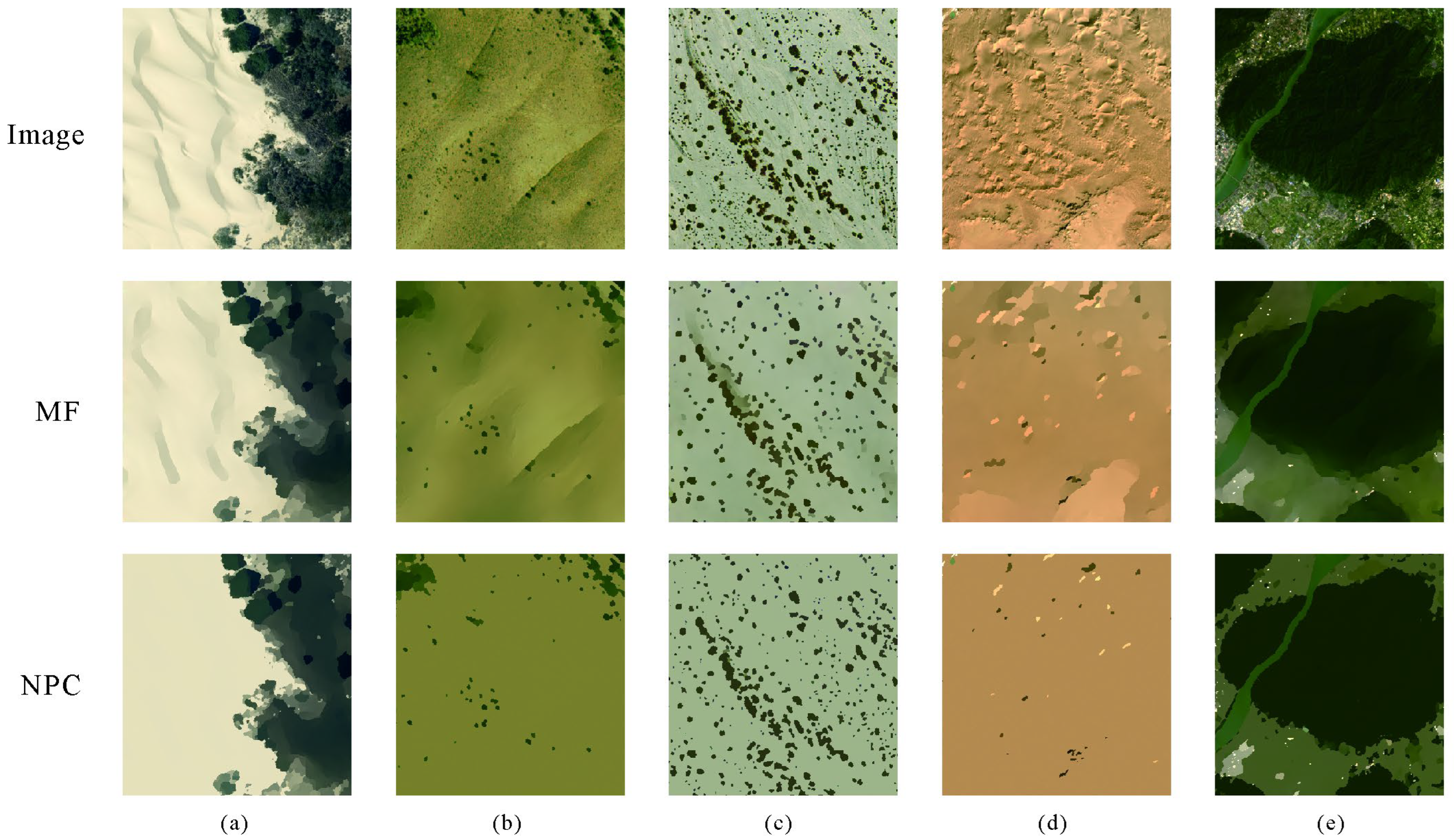
  • An NPC constraint is introduced using a random permutation operator to handle heterogeneous albedo distributions.
  • The adaptability of the SFS-based depth super-resolution is extended, using publicly available global DEM as the initial reference, enabling terrain estimation under more complex surface conditions.
  • High-resolution GF-6 optical satellite data are used for debris-flow erosion volume estimation, and results are quantitatively compared with airborne LiDAR-derived erosion volumes.
The rest of this article is organized as follows. Section 2 presents a comprehensive exposition of the proposed Non-local Piecewise-smooth albedo Constrained SRSFS (NPC SRSFS) algorithm. Section 3 follows with a detailed experimental study and analysis of a debris-flow case in the rural area of Beijing. Finally, Section 4 concludes this article.

2. Methodology

2.1. Background of SRSFS

In this subsection, we provide a brief review of the SRSFS method [33,36] for the general imaging conditions.

2.1.1. Imaging Model

Take the observation data as a multi-band image I c , c = 1 , , C , where C is the number of bands. Suppose the local surface is Lambertian with albedo ρ c , then for an image pixel p , the imaging model is
I c ( p ) = S 2 ρ c ( p ) l c ( ω ) m a x ω n ( p ) , 0 d ω ,
where S 2 d ω is the integration along all incoming light directions ω , S 2 is the unit sphere in R 3 , ρ c ( p ) is the albedo at pixel p of band c , l c is the incoming light radiance, n is the surface normal pointing toward the camera.
To simplify (1), spherical harmonics are introduced. By defining k as
k ( ω , n ) : = m a x ω n ( p ) , 0 ,
(1) can be rewritten in a convolutional form,
I c ( p ) = ρ c ( p ) S 2 k ( ω , n ( p ) ) l c ( ω ) d ω .
With the Funk–Hecke theorem, the spherical harmonic expansion of the integral part in (3) is
S 2 k ( ω , n ( p ) ) l c ( ω ) d ω = n = 0 m = n n k n l n , m c h n , m n ( p ) ,
where h n , m is the orthogonal spherical harmonic basis on the unit sphere, and k n , l n , m c is the expansion coefficients of k , l c , respectively. Under distant lighting conditions, first- or second-order spherical harmonics can make good approximation of incoming radiance.
Substituting (4) into (3), the imaging model can be expressed as
I c ( p ) = ρ c ( p ) l c h n ( p ) ,
where, for second-order spherical harmonic approximation h n ( p ) = 1 , n 1 , n 2 , n 3 , n 1 n 2 , n 1 n 3 , n 2 n 3 , n 1 2 n 2 2 , 3 n 3 2 1 T , l c is the spherical harmonic illumination vector incorporating k n , l n , m c and the constant factor in h n , m . The advantage of using (5) is that the illumination vector l c no longer changes across the spatial domain. The disadvantage is that the relationship with surface normal vector n ( p ) becomes non-linear, which will be addressed later in the numerical optimization procedure. Since each channel of the image can be processed independently, we omit the superscript c for simplicity in the following derivations.

2.1.2. Piecewise Constant Albedo

A piecewise constant constraint is a natural representation of the spatial distribution of ground objects. In the SRSFS framework, albedo is assumed to be piecewise constant with the regularization item ρ 0 . However, directly optimizing the L0-norm constraint item is challenging. To address this, the Mumford–Shah Functional (MF) [42] is employed as an approximation of ρ 0 .Then, taking l h as the shading variable s , the problem of albedo estimation in SRSFS becomes
a rgmin ρ ρ s I 2 2 + R ρ .
The R ρ item represents m i n α 1 ρ 2 , λ 1 , where α 1 , λ 1 are the constants that balance smoothness and the number of significant discontinuities. The problem of (6) can be solved with the primal–dual algorithm. In practice, the accurate estimation of albedo is critical to the success of SRSFS, and the piecewise constant constraint plays a key role in reducing the inherent ambiguity in the SFS problem. The SRSFS algorithm has demonstrated promising results when applied to RGB imagery in computer vision tasks.
However, the piecewise smooth constraint is typically implemented via gradient operators, which only capture local differences between adjacent pixels. The MF constraint, as a local smoothness prior, may inadvertently suppress elongated and isolated structures by misinterpreting them as noise. Moreover, spatially disjoint regions of the same land cover class cannot be constrained as belonging to the same category under such local constraints. This poses a significant challenge for debris-flow studies, as erosion zones often follow elongated patterns along flow paths and are typically situated in local topographic depressions. Due to the limited spatial resolution of commonly used satellite imagery, the narrow upstream areas of erosion zones are only captured by sparse pixels. To overcome these limitations, a novel NPC SRSFS algorithm is proposed in the next subsection to better capture elongated and spatially discontinuous features while preserving meaningful structural patterns.

2.2. NPC SRSFS

Since the gradient-based constraint of SRSFS operates locally, it fails to capture similarities between spatially disconnected regions that may belong to the same class. The non-local prior assumes that regions with similar albedo values are likely to be related, regardless of their spatial proximity. This assumption enables the albedo sparsity prior to enforce global consistency by linking non-adjacent but spectrally similar regions. The non-local means [43] searches across the entire image for similar patches and performs a similarity-weighted average. Random sampling [44] can also associate a given pixel with distant pixels of the same category. This non-local cue becomes particularly effective when combined with the albedo sparsity prior. However, traditional non-local similarity operators (e.g., non-local means, random sampling, and clustering) are inherently non-linear, which complicates the inversion of the albedo estimation problem. To address this, we propose using a random permutation operator as a linear alternative.
A permutation operator is a linear transformation that reorders the elements of a vector or sequence without changing their individual values. Specifically, it preserves vector addition and scalar multiplication, thereby satisfying the properties of linearity. Moreover, the inverse of a permutation operator is straightforward to compute. This simplicity stems from the fact that the inverse operation merely reverses the permutation, restoring the original order of elements. To leverage the benefits of both random sampling and linear transformations, we propose permuting the image array using a random sequence, namely, a random permutation operator, denoted as P . Then, we define ( E P ) as the operator M , where E is the identity operator. Here, M serves as the non-local differential operator that captures differences across randomly sampled, non-local pixel pairs. The corresponding albedo estimation problem with NPC can be formulated as
a r g m i n ρ ρ s I 2 2 + R ρ + G M ρ ,
where R ( ρ ) represents m i n [ α 1 ρ 2 , λ 1 ] , G ( M ρ ) represents m i n [ α 2 M ρ 2 , λ 2 ] , α 1 , α 2 and λ 1 , λ 2 are the constants balancing non-local smoothness and the number of sharp albedo discontinuities. Donate the entire objective function in (7) as J ( ρ ) . Using the Legendre–Fenchel convex conjugate, J ( ρ ) can be expressed as
J ( ρ ) = s u p ρ s I 2 + p , ρ R * ( p ) + q , M ρ G * ( q ) ,
where * is the convex conjugate operator, p , q are the dual variables of ρ , M ρ , respectively. Take the derivative of J ( ρ ) respect to p , q , ρ and set the derivatives to be zeros; the solution can be found using the primal–dual algorithm. With the detailed derivations provided in Appendix A, the complete update procedure for the albedo estimation with NPC is summarized in Algorithm 1.
Algorithm 1 Update of the non-local piecewise smooth constrained albedo.
Input: Image I , parameters α 1 , α 2 , λ 1 , λ 2 , ε , d , where ε is the iteration tolerance, d is the dimensionality of the image, step factors σ , τ
1. Initialize:  ρ = ρ 0 = I , s = 1 , p 0 = q 0 = 0 , τ = 1 2 d , σ = 1 2
%%main loops
2. while  ρ k + 1 ρ k > ε do
         %Dual ascent in   p , q
3.         p ~ = p k + σ ρ
4.         p k + 1 = 2 α 1 σ + 2 α 1 p ~ , p ~ < λ 1 α 1 σ ( σ + 2 α 1 ) 0 , e l s e
5.         q ~ = q k + σ M ρ
6.         q k + 1 = 2 α 2 σ + 2 α 2 q ~ , q ~ < λ 2 α 2 σ ( σ + 2 α 2 ) 0 , e l s e
         %Primal descent in ρ
7.         ρ ~ = ρ k τ T p k + 1 τ M T q k + 1
8.         ρ k + 1 = ρ ~ + 2 τ s I 1 + 2 τ s 2
         %Auxiliary variables update step
9.         θ = 1 1 + 4 τ , τ = θ τ , σ = σ θ , s = I ρ
10.         ρ = ρ k + 1 + θ ρ k + 1 ρ k
end while
Output: albedo ρ
To briefly evaluate the performance of the albedo update algorithm with NPC, we applied it to a series of remote sensing images covering landform types with diverse topographic characteristics. The albedo results obtained through the NPC filtering were compared with those generated by the MF filtering based on local constraints. The comparative results are illustrated in Figure 1. All datasets were sourced from the U.S. Geological Survey Earth Explorer platform (https://earthexplorer.usgs.gov/, accessed on 3 July 2025). Columns (a)–(c) in Figure 1 display 0.3 m high-resolution airborne data, while columns (d)–(e) show Landsat 9 OLI L2 data with a spatial resolution of 30 m. In each subfigure, the first row displays the RGB imagery in the visible spectrum, the second row presents the albedo results obtained using MF filtering, and the third row shows the albedo results from NPC filtering. Figure 1a depicts the sand dunes and surrounding vegetation in Oceano, California, a region with moderate topographic undulations. The hillside scene near Carson City, Nevada, is shown in Figure 1b, characterized by sparse vegetation and moderate terrain relief. Figure 1c illustrates the dry riverbed of Lytle Creek in San Bernardino, California. Sediment deposits shaped by historical water flow introduce subtle terrain variations. Mingsha Mountain near Dunhuang, China, is presented in Figure 1d, where large-scale sand dunes create significant topographic variations. Finally, Figure 1e displays a mountainous region near Zhaoqing, China, where the Xijiang River cuts through complex landscape. The mountains, covered with evergreen broadleaf forests, exhibit significant elevation changes, while agricultural fields and urban areas add to the surface heterogeneity. Overall, across a range of natural landscapes, NPC filtering consistently proves effective in mitigating topographically induced brightness variations, resulting in more uniform albedo distributions than those achieved with MF filtering. Furthermore, it enhances discontinuous but similar surface patches, which benefits the albedo estimation step within the SFS framework.
Due to the ill-posed nature of the SFS problem, additional prior information beyond albedo is required. Specifically, the surface area formed by the depth map is assumed to satisfy a minimal surface constraint [45], supported by a coarse-resolution initial depth. The resulting constrained optimization problem of NPC SRSFS is
min ρ , l , z , θ ρ l h I 2 2 + μ K z z 0 2 2 + ν d A θ 1 + R ρ + G M ρ , s . t . θ = z , z T ,
of which z 0 is the initial low-resolution depth, K is the downsampling matrix for depth values, d A θ is the area of unit surface element, θ is the auxiliary variable. In (9), the first item ρ l h I 2 2 is the data misfit, μ , ν are the weights of depth prior constraint K z z 0 2 2 and minimal surface area constraint d A θ 1 , respectively. Similar to SFSRS, the numerical solution of NPC SRSFS is obtained using the multi-block ADMM algorithm [36]. The whole optimization process terminates either when the estimated depth converges or a predefined maximum number of iterations is reached. The complete procedure of the NPC SRSFS algorithm is summarized in Algorithm 2.
The proposed NPC SRSFS algorithm is compatible with both perspective and orthographic imaging models. However, in the context of remote sensing, available imagery products are typically preprocessed through radiometric calibration, geometric corrections, and orthorectification. Furthermore, the intrinsic parameters of satellite-mounted optical cameras are often inaccessible or undisclosed, with most datasets providing only Rational Polynomial Coefficients (RPCs). As a result, when intrinsic parameters are unavailable, practical implementations of NPC SRSFS generally adopt the orthographic imaging model. The derivation of the orthographic imaging model, along with its associated surface normal and unit surface element formulations, is presented in Appendix A. The following subsection explores the application of the NPC SRSFS algorithm in debris-flow erosion volume estimation.
Algorithm 2 NPC SRSFS.
Input: Image I , low-resolution z 0 , parameters μ , ν , weight of the augmented Lagrangian κ
1. Initialize:  ρ 0 , l 0 , z 0 , θ 0 , u 0
 %%main steps of ADMM
2. while z k + 1 z k z 0 > t o l do
        %Albedo update
3.       Update ρ k + 1 using the primal-dual method as
                     ρ k + 1 = a r g m i n ρ ρ k l k h k I 2 2 + R ρ + G M ρ ,
        %Lighting update
4.       Estimate l k + 1 using pseudo-inverse as
                 l k + 1 = a r g m i n l ρ k + 1 l k h k I 2 2 ,
        %Auxiliary variable update
5.       Update θ k + 1 using L-BFGS as
             θ k + 1 = a r g m i n θ ρ k + 1 l k + 1 h k ( θ ) I 2 2 + ν d A θ 1 + κ 2 z , z k θ k + u k 2 2 ,
        %Depth update
6.       Refine z k + 1 by the conjugate gradient method as
               z k + 1 = a r g m i n z μ K z k z 0 2 2 + κ 2 z , z k θ k + 1 + u k 2 2 ,
        %Extrapolation step
7.       Perform u k + 1 extrapolation as
                 u k + 1 = u k + z , z k + 1 θ k + 1 .
end while
Output: estimated ρ , l , z

2.3. Debris-Flow Erosion Volume Estimation

Debris flows primarily exert their destructive impact within localized regions, which can be categorized into erosion and deposition zones based on topographic differences before and after the event. The magnitude of a debris flow is closely related to the volume of the eroded zone. The affected regions often exhibit distinct surface albedo characteristics compared to the surrounding terrain. The proposed NPC SRSFS algorithm enables terrain reconstruction in debris-flow regions by accounting for albedo variations across the entire image. Using high-resolution post-disaster optical satellite imagery and incorporating Global DEM (GDEM) as an initial depth prior, the post-event DSM can be estimated. With the GDEM products offering resolutions of 30 m or finer, reliable baseline elevation data are readily accessible. If pre-disaster satellite imagery is available, it can also be processed using the same method to estimate a pre-event DSM. In its absence, the GDEM can be interpolated to approximate the terrain prior to the disaster. By comparing the DSMs before and after the event, changes in terrain elevation can be directly extracted, enabling quantitative estimation of erosion volume.
In addition to the primary debris-flow body, adjacent regions may also experience landslides or collapses of varying scales. Moreover, vegetation cover on mountainous slopes may introduce minor elevation changes between observation periods. To isolate debris-flow-affected areas, a basic land cover classification is first performed using the k-means clustering algorithm, distinguishing disturbed surfaces from undisturbed terrain. To further refine this classification, a manually defined Region of Interest (ROI) is applied to delineate the erosion mask more precisely. The complete procedure for estimating debris-flow erosion volume is outlined in Algorithm 3.
Algorithm 3 Debris-flow erosion volume estimation.
Input: Post-disaster image, Pre-disaster image (optional), GDEM
Main steps:
        %Post-disaster image processing
1.        Generate the debris-flow area mask
2.        Estimate the post-disaster DSM using NPC SRSFS
        %Pre-disaster image processing (optional)
3.        Estimate the pre-disaster DSM using NPC SRSFS (or simply interpolate from GDEM)
        %DSM differencing
4.        Compute the difference between post-disaster and pre-disaster DSMs
        %Volume calculation
5.        Calculate debris-flow erosion volume within the left area
Output: estimated debris-flow erosion volume

3. Experiments and Discussion

Climate change has significantly increased the risk of debris-flow events, with extreme precipitation and post-wildfire rainfall emerging as major triggers. Unlike remote regions, urban-adjacent areas benefit from more frequent satellite observations, offering a practical advantage for geohazard monitoring. High-resolution satellite imagery facilitates the precise identification of fine-scale debris-flow features, accurate delineation of affected zones, and reliable estimation of erosion volume. Accordingly, this study focuses on the mountainous regions surrounding Beijing, leveraging high-resolution satellite imagery for accurate debris-flow erosion volume estimation.

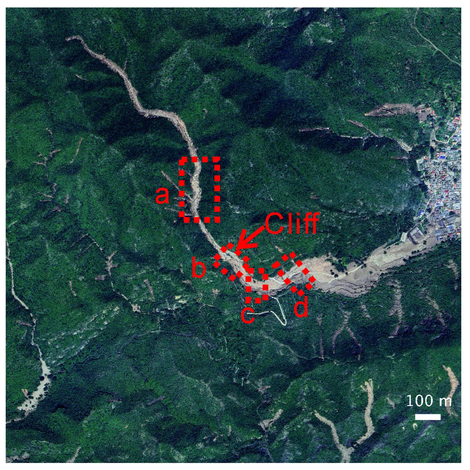
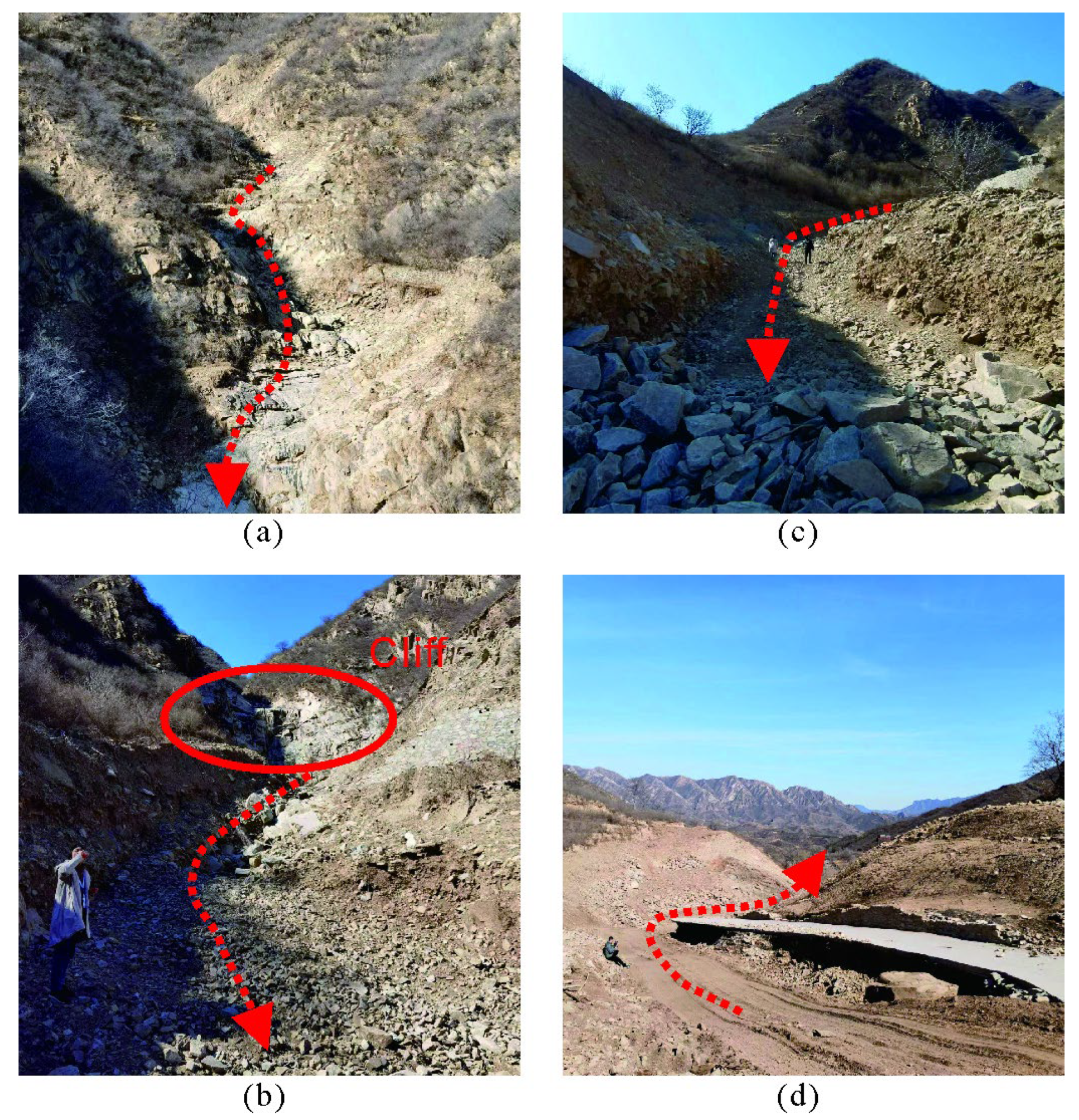
3.1. Research Area and Datasets

Beijing is situated at the intersection of the Yan Mountains and the Taihang Mountains, featuring a terrain that slopes from high elevations in the northwest to lower elevations in the southeast. The mountainous regions of Beijing, dominated by low to mid-elevation hills, are highly susceptible to geological hazards. In recent years, the frequency of extreme rainfall events has increased. Notably, between 20:00 on 29 July and 07:00 on 2 August 2023, Beijing experienced an extreme rainstorm caused by Typhoon Doksuri [46]. Within just 83 h, the citywide average rainfall reached 331 mm, equivalent to 60% of the annual average precipitation. The hardest-hit areas included Mentougou District, with an average of 538.1 mm of rainfall, and Fangshan District, with 598.7 mm. The disaster caused 33 fatalities and left 18 people missing. The extreme rainstorm also triggered debris-flow events.
The study area is located in Mentougou District of western Beijing, a region renowned for its rich natural landscapes and cultural heritage. Mentougou features mountainous terrain with significant elevation variations. These topographical conditions make the area highly susceptible to debris flows during heavy rainfall. Using the China land cover dataset [47], Figure 2a illustrates Beijing’s administrative map, highlighting the dense vegetation coverage in the western and northern mountainous regions, while impervious surfaces are concentrated in the urban core. The administrative boundaries of Mentougou are outlined in black. The selected study area, outlined by the black box in Figure 2b, lies within Mentougou. The figure also shows that impervious surfaces are more concentrated in the eastern areas adjacent to the urban center, while the majority of the district comprises mountainous terrain covered by vegetation.
Considering that debris-flow events in Beijing are generally of small to medium scale, the width of the upstream erosion zones is typically only a few meters. To effectively monitor the fine-scale erosion features, high-spatial resolution optical satellite imagery is essential. Among the available data sources, China’s GF series satellites, primarily GF-1, GF-2, and GF-6, offer suitable imagery. GF-6 has enhanced imaging capabilities compared to GF-1 and GF-2, including a 2 m panchromatic/8 m multispectral camera with a 90 km swath [19]. It primarily supports precision agriculture and ecological monitoring. For this study, high-resolution multispectral data from the PMS camera onboard the GF-6 satellite were chosen (https://data.cresda.cn/#/home, accessed on 3 July 2025). Images acquired on 5 July (pre-event) and 19 August 2023 (post-event) were selected based on a cloud cover threshold of less than 5% during the July–August 2023 period to ensure minimal obstruction of ground features.
The Level-1A satellite data were geometrically corrected using RPCs and orthorectified. Additionally, pan-sharpening merged the panchromatic and multispectral bands, generating high-resolution RGB and near-infrared images with 2 m resolution. These images served as the input for subsequent analysis. On-site observations and satellite imagery confirmed that a notable debris-flow event occurred near Lingshui Village, Mentougou District. Figure 2c presents pre-disaster imagery of the mountainous terrain near Lingshui village, while Figure 2d displays the corresponding post-disaster scene. Lingshui Village is located in the upper-right section of both images. A comparison of the pre- and post-disaster imagery clearly reveals the debris-flow-affected areas and minor flow traces on adjacent slopes. The debris flow was caused by sustained heavy rainfall at the end of July 2023. Prior to the event, a strong rainfall warning prompted the village to implement evacuation measures. The affected area suffered significant damage, with erosion concentrated in the upstream mountainous regions. As the terrain gradually flattened toward the downstream village area, the debris flow lost momentum, leading to sediment deposition and the spread of debris-laden slurry. This transition caused considerable damage to buildings and blocked most of the roads. After the disaster, the village underwent prolonged cleanup efforts to reduce impacts and prevent secondary hazards.
For comparison, a 0.3 m post-disaster image from Google Earth (GE) is presented in Figure 3 (https://earth.google.com/, accessed on 3 July 2025), clearly showing severe upstream erosion. In March 2024, we conducted an on-site survey, capturing photographs along the debris-flow path at locations marked as points (a-d) in Figure 3. Corresponding ground-level photographs in Figure 4 document the progressive geomorphic changes caused by the debris flow. In Figure 4a, near the source, the debris-flow channel appears relatively narrow, indicating initial erosion. Moving forward, Figure 4b shows a sudden drop in terrain, which significantly increased flow energy and erosive force. Figure 4c depicts intense erosion along the valley floor and adjacent slopes, reflecting the high-energy impact of the flow. Finally, Figure 4d captures the site where a mountain road was destroyed. Beyond this point, the terrain widens and flattens, leading to a gradual reduction in erosive force as the debris flow approached the village.
Pre- and post-disaster airborne LiDAR data within the study area are collected to establish ground truth DSMs. The raw point cloud data from the airborne LiDAR were processed through automatic filtering, classification, and manual refinement to remove moving objects and overhead power lines, resulting in 2 m DSM products. The pre-disaster LiDAR data were acquired in May 2023 as part of an urban mapping project, while the post-disaster LiDAR data were collected in October 2023 during a disaster assessment project.

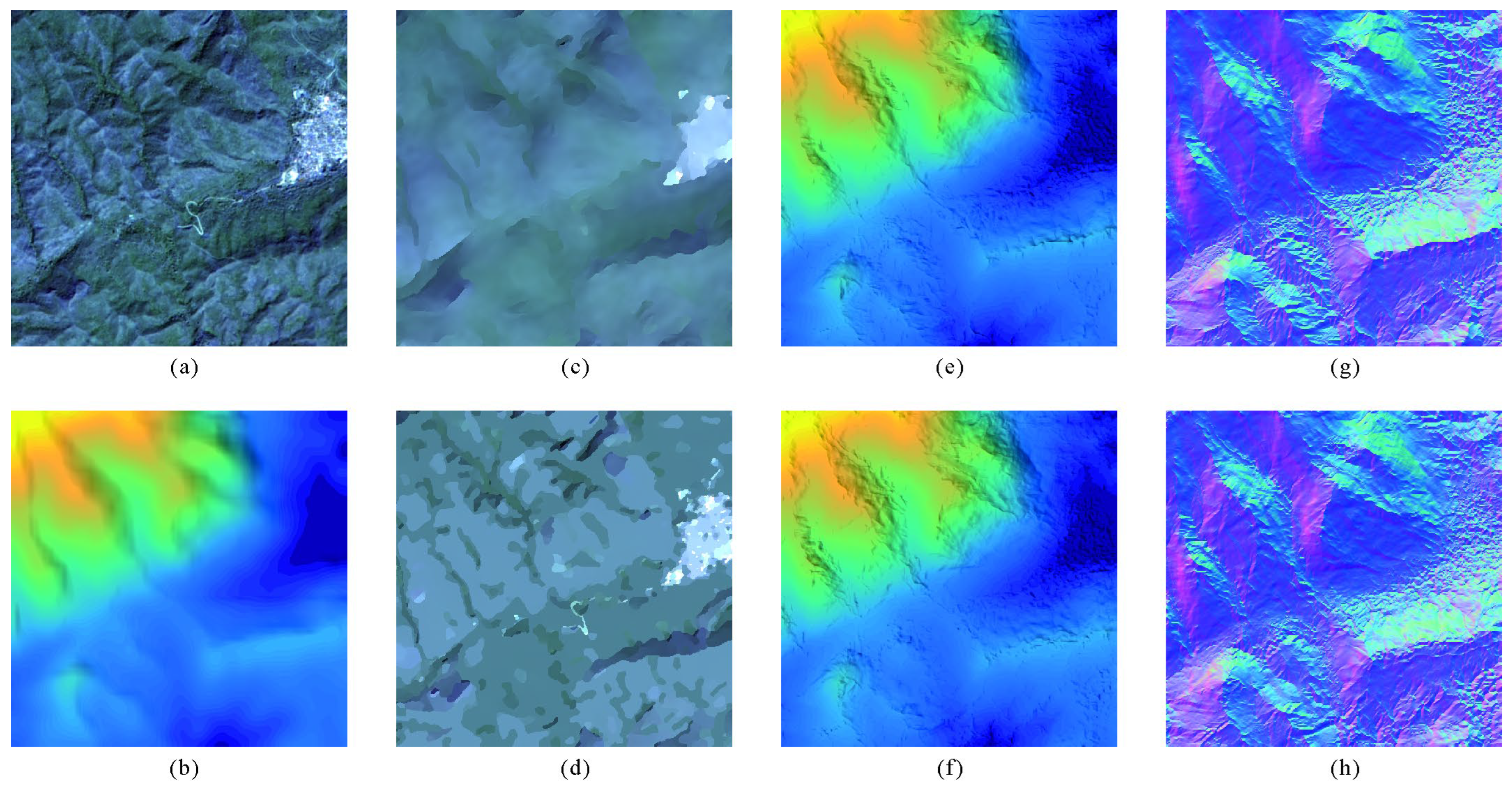
3.2. Experimental Results

In optical remote sensing imagery, vegetation-covered slopes affected by collapse are generally identifiable, making erosion zones of debris flows relatively easier to detect with relatively uniform apparent reflectance. However, deposition zones are more challenging to distinguish, as widespread sediment deposits often resemble other surface features such as buildings, bare ground, and infrastructure. Quantifying the volume of deposited material is also difficult, particularly when debris infiltrates buildings. This challenge is further compounded by the fact that cleanup operations usually begin soon after the disaster in residential areas, obscuring the original deposition patterns, whereas upstream eroded surfaces tend to remain more stable over time, allowing for more reliable volume estimation. The scale of a debris-flow event is directly correlated with the volume of eroded material. Therefore, we focus on the estimation of the erosion volume of the debris-flow. Using the proposed NPC SRSFS algorithm, we reconstruct high-resolution DSMs from single high-resolution satellite images, with the publicly available SRTM DEM (https://earthexplorer.usgs.gov/, accessed on 3 July 2025) used as the initial terrain reference.
Refined DSMs were reconstructed using both the SRSFS algorithm and the proposed NPC SRSFS algorithm based on pre- and post-disaster GF-6 images. To ensure a fair comparison, both methods were tuned to their respective optimal parameter settings. Figure 5 and Figure 6 present the estimated albedo and DSM results derived from the pre- and post-disaster GF-6 images, respectively. The SRTM DEM was used as initial elevation. Given the large elevation range in the DSMs, terrain normals were computed to better visualize subtle topographic variations. The x, y, and z components of the surface normals were mapped to RGB channels to enhance terrain features.
The pre-disaster GF-6 image is shown in Figure 5a, while the corresponding SRTM DEM is displayed in Figure 5b. Comparing the albedo map derived from the SRSFS method and the proposed NPC SRSFS method (see Figure 5c,d), the latter exhibits improved adaptability to spatially varying surface characteristics. It preserves sharper object boundaries and avoids the over-smoothing observed in the SRSFS result. The DSMs reconstructed by both methods (see Figure 5e,f) reveal similar terrain features. Meanwhile, the surface normals (see Figure 5g,h) indicate that, in the absence of significant pre-disaster terrain changes, both approaches produce comparable elevation models.
Figure 6a highlights the post-disaster scene, where the debris-flow area is clearly distinguishable due to its altered reflectance properties. Using the same initial DEM (see Figure 6b), the albedo produced by NPC SRSFS (Figure 6d) again outperforms that of SRSFS (Figure 6c) by preserving more structural details and better capturing land cover heterogeneity. Although the DSMs in Figure 6e,f appear visually similar, more subtle differences emerge in the surface normals displayed in Figure 6g,h. In the upstream sections of the debris flow, both methods yield comparable DSM results. However, a notable terrain difference is observed after zone (b) in Figure 3, corresponding to the primary impact zone of the debris flow. In these regions marked by red dashed ellipses, NPC SRSFS is more effective at capturing fine-scale morphological variations, whereas SRSFS tends to smooth out or miss these details.
To further compare the performance of SRSFS and NPC SRSFS, debris-flow erosion was estimated by subtracting the pre-disaster DSM from the post-disaster DSM. The debris-flow mask was generated by combining k-means clustering, which separates vegetated and non-vegetated areas in the post-disaster GF-6 image, with a manually delineated ROI representing the approximate extent of debris-flow activity. To focus on the primary erosion zone and exclude minor peripheral flows and downstream deposition near the village, the analysis was constrained to the area enclosed by the red dashed rectangle in Figure 6a. Figure 7 presents the erosion estimates derived from satellite imagery. In Figure 7a, the debris-flow mask is overlaid in semi-transparent red on the post-disaster GF-6 image. Figure 7b,c show the erosion patterns estimated by SRSFS and NPC SRSFS, respectively, within the masked region outlined in white. The main differences between the two methods appear after the cliff marked in Figure 3, where a sharp elevation drop generates significant gravitational potential energy, leading to intense erosion. This observation is supported by a field survey.
Although the proposed NPC SRSFS method generally provides improved terrain reconstruction accuracy, some localized discrepancies are observed. Specifically, the method tends to underestimate erosion in the upstream sections. This is primarily due to the narrow width of the erosion channel in the upper reaches, which poses a significant challenge for accurate reconstruction when using satellite imagery with limited spatial resolution. Fine-scale geomorphic changes in such confined areas are difficult to resolve reliably without ultra-high-resolution data. Conversely, in the right bank of the downstream region, the method tends to overestimate erosion. This area lies on the shaded side of the slope, where topographic shadows occur in the optical image. Due to the limitations of SFS-based models under low-illumination or shadow conditions, reliable reflectance-based terrain estimation becomes challenging. In such cases, the optimization is strongly influenced by the smoothness constraints and information propagated from better-illuminated regions, particularly the left bank, which may result in an overestimation artifact.
Nevertheless, in the main debris-flow erosion zone, where surface reflectance remains relatively homogeneous, the NPC SRSFS approach demonstrates superior performance. Its use of non-local constraints allows it to better capture subtle terrain changes within areas of consistent albedo, a capability less pronounced in the baseline SRSFS model. As a result, the NPC SRSFS method provides more accurate erosion estimation in the core impact area of the debris-flow event.
To validate the estimated erosion volumes of the debris flow, we used airborne LiDAR data to establish a ground truth reference. Figure 8a,b display the DSMs generated from the pre- and post-disaster airborne LiDAR point clouds, respectively, with rich details. A debris-flow impact area mask was created using the previously described mask generation method on the GE image and resampled to 2 m. By subtracting the pre-disaster DSM from the post-disaster one, the erosion pattern within the masked area was derived, as shown in Figure 8c. The white boundary indicates the primary debris-flow-affected region. The erosion data derived from airborne LiDAR clearly reflect the erosion from the source area down to the village. However, since the post-disaster LiDAR data were collected several months after the event, parts of the affected area near the village had undergone manual leveling and cleanup, potentially causing disturbance to the ground truth.
For a quantitative comparison of estimated erosion, we computed the debris-flow erosion volumes within the impacted area. Table 1 summarizes the results obtained using the SRSFS method, the proposed NPC SRSFS method, and airborne LiDAR data, which serves as the ground truth. The percentage relative error is calculated as
R e l a t i v e   E r r o r % = V E s t i m a t e d V L i D A R V L i D A R × 100 % ,
where V E s t i m a t e d is the erosion volume estimated from the SRSFS or NPC SRSFS method, and V L i D A R is the reference erosion volume derived from airborne LiDAR data. The SRSFS method substantially underestimates the erosion volume, with relative errors of −47.78% and −40.45% when using the post-event DSM (generated from post-disaster optical imagery) combined with the GDEM and the pre-disaster DSM (generated from pre-disaster optical imagery) as references, respectively. Conversely, the proposed NPC SRSFS method achieves considerably improved accuracy, with relative errors of +6.72% and +9.57% under the same conditions, producing estimates that closely align with the LiDAR-derived reference volume of 99.71 × 10³ m3.
It is worth noting that, whether SRSFS or NPC SRSFS is used to estimate debris-flow erosion volumes, employing the GDEM as pre-disaster DSM consistently results in a lower erosion volume estimate than using the DSM derived from pre-disaster imagery. This is expected, as the GDEM excludes surface vegetation and thus generally provides lower elevation values than image-derived DSMs. As a result, the estimated erosion volume using GDEM as the pre-disaster DSM is smaller. For NPC SRSFS, the estimated erosion volume is slightly higher than that derived from the LiDAR data. This discrepancy may be attributed to the timing of data acquisition. The post-disaster satellite imagery was captured in August, whereas the airborne LiDAR survey was conducted in October. By the time of the LiDAR acquisition, the debris-flow area near the village may have already been partially cleared or leveled, leading to a slight underestimation of erosion volume in the LiDAR-derived results. This also emphasizes the importance of conducting post-disaster assessments as early as possible. Moreover, the proposed method enables debris-flow erosion estimation using a monocular post-disaster optical image, which requires minimal satellite data and facilitates rapid assessment.
Furthermore, the deviation of erosion volume between the NPC SRSFS and LiDAR-derived estimates remains within 10%, demonstrating the method’s reliability in debris-flow volume estimation. NPC SRSFS delivers accurate and robust results, regardless of whether the pre-event DSM is GDEM or derived from pre-disaster imagery. These results demonstrate the effectiveness of the proposed method for terrain reconstruction and debris-flow erosion volume estimation. The estimated erosion volume, close to 100,000 m3, confirms this event as a medium to large-scale debris flow with considerable destructive capacity. An event of this magnitude is rarely documented in the mountainous regions near Beijing. This further highlights the critical need for robust debris-flow monitoring and accurate terrain reconstruction, especially in high-risk suburban and mountainous areas surrounding large urban centers.

3.3. Parameter Analysis

Like most variational optimization models, the NPC SRSFS algorithm requires proper parameter tuning to achieve optimal performance. The optimal value of the parameters μ , ν , λ 1 , λ 2 can theoretically be selected based on the noise characteristics of each term in (11). However, such parameter tuning can be challenging when applied to real-world data. Based on experiments conducted on synthetic data, the parameter set μ , ν , λ 1 , λ 2 = ( 0.1,0.7,0.5,0.25 ) yields satisfactory albedo estimation results. These values are adopted across all experimental cases. To assess the robustness of the algorithm with respect to these parameters, we performed a grid search using the Mentougou case study. The sensitivity analysis primarily focuses on the influence of λ 1 , λ 2 on the final erosion volume estimation. Specifically, we varied λ 1 from 0.1 to 1.0 and λ 2 from 0.05 to 0.5. For each parameter combination, we computed the erosion volume by differencing the post- and pre-disaster DSMs.
The results in Figure 9a show that the estimated erosion volume fluctuates within the range of approximately 90 to 115 × 103 m3. Parameter combinations near the center of the heatmap result in more stable and consistent volume estimates. Based on empirical experience, the default setting of λ 1 , λ 2 = ( 0.5,0.25 ) generally produces robust results. This analysis confirms that the proposed method exhibits strong robustness to moderate variations in λ 1 , λ 2 , and supports the reliability of the erosion volume estimation.
The final DSM reconstruction in our framework is jointly determined by both albedo estimation and depth inference, with the initial depth information playing a crucial role in guiding the optimization toward a physically plausible solution and avoiding convergence to poor local minima. The SRTM DEM is selected as the initial reference primarily due to its global availability and accessibility, which aligns with our goal of proposing a rapid post-disaster assessment method that minimizes dependence on auxiliary data.
To further assess how the resolution of the initial DEM affects the accuracy of erosion volume estimation, we conducted a sensitivity experiment using the Mentougou case. Specifically, we used resampled versions of LiDAR DSMs at 30 m, 20 m, 10 m, 5 m, and 2 m resolution, in addition to the original SRTM DEM, as initial inputs for the NPC SRSFS algorithm. We then computed pre- and post-disaster DSMs and their differences to estimate erosion volume. The results are presented in Figure 9b. The comparison indicates that higher-resolution initial DEMs lead to slightly more accurate erosion volume estimates. Nevertheless, the method still delivers acceptable accuracy even with a coarse 30 m initial DEM. This confirms that the SRTM DEM, despite its lower resolution, is a viable and practical choice for initial elevation input in scenarios where only single pre- and post-event images are available.
To evaluate computational efficiency, the proposed NPC SRSFS algorithm was implemented in MATLAB R2016b without GPU acceleration. All experiments were conducted on a laptop equipped with a 12th Gen Intel(R) Core(TM) i7-1280P CPU (1.80 GHz) (Intel Corporation, Santa Clara, CA, USA). The complete processing time for the DSM reconstruction was approximately 316 s. Given the high-resolution outputs and minimal data requirements, this runtime is considered acceptable for post-disaster rapid assessment scenarios.

4. Conclusions

This study investigates the feasibility of estimating debris-flow erosion volume using a single post-disaster high-resolution optical image and proposes a Shape from Shading approach with NPC SRSFS. By leveraging high-resolution optical satellite imagery and publicly available global DEM data, this method enables accurate post-disaster terrain reconstruction without the need for stereo imagery, significantly reducing data requirements and supporting rapid disaster assessment. The results demonstrate that the DSM reconstructed from a monocular image can effectively capture topographic changes, supporting the quantitative estimation of debris-flow erosion volume. While the current application focuses on post-event debris-flow evaluation and geomorphic change detection, the approach also shows potential for other applications such as landslide monitoring and ice crevasse analysis. Compared to conventional ground surveys and aerial photogrammetry, the proposed method offers a novel way for disaster assessment. Due to the limited availability of ground truth data, the experiment focused on a single debris-flow event in Beijing. Despite challenges related to complex surface reflectance variability and initial DSM accuracy, the method performed well in a medium-scale debris-flow case, providing reliable, quantitative information for post-disaster assessment.
The accuracy of the estimated erosion volume may be influenced by surface cover conditions. In particular, dense vegetation or man-made structures present in the debris-flow source area prior to the event may reduce the accuracy of pre-disaster DSM estimation. After the event, the relative homogeneity of the eroded surface may also affect the quality of post-disaster DSM reconstruction. These factors can lead to potential errors in the final erosion volume estimates. It is also important to note that the proposed method assumes adequate illumination over the debris-flow-affected area. Most of the eroded zones should be directly exposed to sunlight for reliable albedo and depth estimation. The method is not suitable for areas entirely in shadow or submerged under water, where reliable estimation cannot be ensured.
In addition, this study focuses on a medium-scale debris-flow case. For small-scale debris flows, monitoring remains challenging due to the limited spatial resolution of satellite imagery. Conversely, large-scale debris flows often involve more complex processes, including a combination of collapse, landsliding, erosion, and deposition across different zones. Moreover, field investigation and collection of accurate ground truth data for such events require significantly more resources, which were beyond the scope of this study.
Future work may further improve the accuracy and applicability of the proposed method by incorporating multi-source remote sensing data and advanced deep learning techniques.

Author Contributions

Conceptualization, P.Z. and G.Z.; methodology, P.Z., S.W. and G.Z.; software, P.Z.; validation, P.Z., Y.Z. and L.J.; formal analysis, P.Z.; investigation, P.Z., Y.Z., K.L. and L.J.; resources, Y.Z. and L.J.; data curation, S.W. and K.L.; writing—original draft preparation, P.Z.; writing—review and editing, P.Z., S.W. and G.Z.; visualization, P.Z. and S.W.; supervision, G.Z.; funding acquisition, G.Z. All authors have read and agreed to the published version of the manuscript.

Funding

This research was funded by the National Key Research and Development Program of China, grant number 2023YFF1303802.

Data Availability Statement

Data are contained within the article.

Conflicts of Interest

The authors declare no conflicts of interest.

Appendix A

Appendix A.1. Orthographic Camera Model

Take the camera’s pupil center O as the origin of the world coordinates system. The center of the image plane is denoted as O , as in Figure A1. The horizontal and vertical directions on the image plane are marked as u , v , respectively. The x , y axes of the world coordinate system are parallel to u , v , and the z axis is perpendicular to the x y plane, pointing towards the ground. For the orthographic camera model, the relationship between a point on the ground surface and its corresponding projection on the image plane is
X ( u , v ) = u v z ( u , v ) .
The surface normal at point X is parallel to u X × v X . Then, we obtain
u X × v X = i j k 1 0 z u 0 1 z v = z u z v 1 .
Since the surface normal points towards the camera, it can be expressed as
n ~ = z u ( u , v ) z v ( u , v ) 1 .
The area of a surface element is just the magnitude of u X × v X , which is
d A = z u 2 ( u , v ) + z v 2 ( u , v ) + 1 .
The normalized surface normal is
n = 1 d A z u ( u , v ) z v ( u , v ) 1 .
Figure A1. Orthographic camera model.
Remotesensing 17 02413 g0a1

Appendix A.2. Update of Albedo with NPC

Take the derivative of J ( ρ ) in (8) with respect to p , q , ρ and set the derivatives to be zeros. For p , we have
J ( ρ ) p = ρ R * = 0 p + σ ρ = p + σ R * p = p r o x σ , R * p + σ ρ = p r o x σ , R * p ~ ,
where p r o x is the proximal operator. Using Moreau’s identity, we can get
p r o x σ , R * p ~ = p ~ σ p r o x 1 σ , R p ~ σ .
Consider the general case
p r o x τ , R g ~ = a r g m i n g g g ~ 2 2 2 τ + m i n α 1 g 2 2 , λ 1 ,
with the objective function in (A8) denoted as J 1 . Take the derivative of J 1 with respect to g , then,
J 1 g = g g ~ τ + 2 α 1 g , g < λ 1 α 1 0 , e l s e = 0 g = 1 1 + 2 τ α 1 g ~ , g ~ < λ 1 α 1 1 + 2 τ α 1 g ~ , e l s e .
Substituting (A9) into (A7), we obtain
p r o x σ , R * p ~ = p ~ σ 1 1 + 2 α 1 σ p ~ σ , p ~ < λ 1 α 1 σ σ + 2 α 1 σ p ~ σ , e l s e p = 2 α 1 σ + 2 α 1 p ~ , p ~ < λ 1 α 1 σ σ + 2 α 1 0 , e l s e = p ~ , p ~ < 2 λ 1 σ , f o r   l a r g e   α 1 0 , e l s e .
Similarly, defining q ~ = q + σ M ρ , the solution of q follows the same process by replacing variable p with q ,
q = 2 α 2 σ + 2 α 2 q ~ , q ~ < λ 2 α 2 σ ( σ + 2 α 2 ) 0 , e l s e = q ~ , q ~ < 2 λ 2 σ , f o r   l a r g e   α 2 0 , e l s e .
For the solution of ρ , we have
J ( ρ ) ρ = 2 s ρ s I + T p + M T q = 0 .
Marking 2 s ρ s I as D , it is straightforward to show that
τ T p τ M T q = τ D ρ τ T p τ M T q = ρ + τ D ρ = p r o x τ , D ρ τ T p τ M T q ρ = a r g m i n ρ ρ ρ ~ 2 2 2 τ + D ρ ,
where ρ ~ = ρ τ T p τ M T q . Again, taking the derivative of the objective function above, we get
ρ ρ ~ τ + 2 s ρ s I = 0 ρ ρ ~ + 2 τ s ρ s I = 0 ρ 1 + 2 τ s 2 = ρ ~ + 2 τ s I ρ = ρ ~ + 2 τ s I 1 + 2 τ s 2 .

References

  1. Metternicht, G.; Hurni, L.; Gogu, R. Remote sensing of landslides: An analysis of the potential contribution to geo-spatial systems for hazard assessment in mountainous environments. Remote Sens. Environ. 2005, 98, 284–303. [Google Scholar] [CrossRef]
  2. Jakob, M.; Hungr, O. Debris-Flow Hazards and Related Phenomena; Springer: Berlin/Heidelberg, Germany, 2005; Volume 739. [Google Scholar]
  3. Arattano, M.; Bertoldi, G.; Cavalli, M.; Comiti, F.; D’Agostino, V.; Theule, J. Comparison of Methods and Procedures for Debris-Flow Volume Estimation. In Engineering Geology for Society and Territory, Vol 3: River Basins, Reservoir Sedimentation and Water Resources; Springer International Publishing: Geneva, Switzerland, 2015; pp. 115–119. [Google Scholar] [CrossRef]
  4. Schimmel, A.; Coviello, V.; Comiti, F. Debris flow velocity and volume estimations based on seismic data. Nat. Hazards Earth Syst. Sci. 2022, 22, 1955–1968. [Google Scholar] [CrossRef]
  5. Zhu, L.; Jia, Y.; Huang, S.; Meyer, N.; Wieser, A.; Schindler, K.; Aaron, J. DeFlow: Self-supervised 3D Motion Estimation of Debris Flow. In Proceedings of the IEEE/CVF Conference on Computer Vision and Pattern Recognition, Vancouver, BC, Canada, 17–24 June 2023; pp. 6508–6517. [Google Scholar]
  6. Orland, E.; Kirschbaum, D.; Stanley, T. A Scalable Framework for Post Fire Debris Flow Hazard Assessment Using Satellite Precipitation Data. Geophys. Res. Lett. 2022, 49, 1–9. [Google Scholar] [CrossRef]
  7. He, C.; Ye, B. Automatic Extraction of Potential Debris Flow Based on Gf-2 Satellite Data. In Proceedings of the 2019 IEEE International Geoscience and Remote Sensing Symposium (Igarss 2019), Yokohama, Japan, 28 July–10 August 2019; pp. 9705–9708. [Google Scholar] [CrossRef]
  8. Miura, H. Fusion Analysis of Optical Satellite Images and Digital Elevation Model for Quantifying Volume in Debris Flow Disaster. Remote Sens. 2019, 11, 1096. [Google Scholar] [CrossRef]
  9. Li, Y.; Ma, C.; Wang, Y. Landslides and debris flows caused by an extreme rainstorm on 21 July 2012 in mountains near Beijing, China. Bull. Eng. Geol. Environ. 2017, 78, 1265–1280. [Google Scholar] [CrossRef]
  10. Huang, J.; Hales, T.C.; Huang, R.; Ju, N.; Li, Q.; Huang, Y. A hybrid machine-learning model to estimate potential debris-flow volumes. Geomorphology 2020, 367, 107333. [Google Scholar] [CrossRef]
  11. Hu, X.; Yang, F.; Hu, K.; Ding, M.; Liu, S.; Wei, L. Estimating the debris-flow magnitude using landslide sediment connectivity, Qipan catchment, Wenchuan County, China. Catena 2023, 220, 106689. [Google Scholar] [CrossRef]
  12. Ding, C.; Feng, G.; Liao, M.; Tao, P.; Zhang, L.; Xu, Q. Displacement history and potential triggering factors of Baige landslides, China revealed by optical imagery time series. Remote Sens. Environ. 2021, 254, 112253. [Google Scholar] [CrossRef]
  13. Chen, J.; Zhang, J.; Wu, T.; Hao, J.; Wu, X.; Ma, X.; Zhu, X.; Lou, P.; Zhang, L. Activity and Kinematics of Two Adjacent Freeze–Thaw-Related Landslides Revealed by Multisource Remote Sensing of Qilian Mountain. Remote Sens. 2022, 14, 5059. [Google Scholar] [CrossRef]
  14. Jia, H.; Wang, Y.; Ge, D.; Deng, Y.; Wang, R. Improved offset tracking for predisaster deformation monitoring of the 2018 Jinsha River landslide (Tibet, China). Remote Sens. Environ. 2020, 247, 111899. [Google Scholar] [CrossRef]
  15. Cucchiaro, S.; Maset, E.; Fusiello, A.; Cazorzi, F. 4d-Sfm Photogrammetry for Monitoring Sediment Dynamics in a Debris-Flow Catchment: Software Testing and Results Comparison. Int. Arch. Photogramm. Remote Sens. Spat. Inf. Sci. 2018, XLII-2, 281–288. [Google Scholar] [CrossRef]
  16. Miura, H.; Tanizaki, T. UAV Observations for Soil Volume Estimation of Debris Flows. In Proceedings of the IGARSS 2022––2022 IEEE International Geoscience and Remote Sensing Symposium, Kuala Lumpur, Malaysia, 17–22 July 2022; pp. 7771–7774. [Google Scholar]
  17. Liang, R.; Dai, K.; Xu, Q.; Pirasteh, S.; Li, Z.; Li, T.; Wen, N.; Deng, J.; Fan, X. Utilizing a single-temporal full polarimetric Gaofen-3 SAR image to map coseismic landslide inventory following the 2017 Mw 7.0 Jiuzhaigou earthquake (China). Int. J. Appl. Earth Obs. Geoinf. 2024, 127, 103657. [Google Scholar] [CrossRef]
  18. Wang, S.; Yang, B.; Zhou, Y.; Wang, F.; Zhang, R.; Zhao, Q. Three-dimensional information extraction from GaoFen-1 satellite images for landslide monitoring. Geomorphology 2018, 309, 77–85. [Google Scholar] [CrossRef]
  19. Chen, L.; Letu, H.; Fan, M.; Shang, H.; Tao, J.; Wu, L.; Zhang, Y.; Yu, C.; Gu, J.; Zhang, N.; et al. An Introduction to the Chinese High-Resolution Earth Observation System: Gaofen-1~7 Civilian Satellites. J. Remote Sens. 2022, 2022, 9769536. [Google Scholar] [CrossRef]
  20. Wang, P.; Shi, L.; Chen, B.; Hu, Z.; Qiao, J.; Dong, Q. Pursuing 3-D scene structures with optical satellite images from affine reconstruction to Euclidean reconstruction. IEEE Trans. Geosci. Remote Sens. 2022, 60, 1–14. [Google Scholar] [CrossRef]
  21. Hu, Z.; Tao, P.; Long, X.; Wang, H. Shading aware DSM generation from high resolution multi-view satellite images. Geo-spatial Inf. Sci. 2022, 27, 398–407. [Google Scholar] [CrossRef]
  22. Mertan, A.; Duff, D.J.; Unal, G. Single image depth estimation: An overview. Digit. Signal Process. 2022, 123, 103441. [Google Scholar] [CrossRef]
  23. Shao, J.; Yang, Y.; Zhou, H.; Zhang, Y.; Shen, Y.; Guizilini, V.; Wang, Y.; Poggi, M.; Liao, Y. Learning temporally consistent video depth from video diffusion priors. In Proceedings of the Computer Vision and Pattern Recognition Conference, Nashville, TN, USA, 11–15 June 2025; pp. 22841–22852. [Google Scholar]
  24. Xu, H.; Peng, S.; Wang, F.; Blum, H.; Barath, D.; Geiger, A.; Pollefeys, M. Depthsplat: Connecting gaussian splatting and depth. In Proceedings of the Computer Vision and Pattern Recognition Conference, Nashville, TN, USA, 11–15 June 2025; pp. 16453–16463. [Google Scholar]
  25. Ke, B.; Obukhov, A.; Huang, S.; Metzger, N.; Daudt, R.C.; Schindler, K. Repurposing diffusion-based image generators for monocular depth estimation. In Proceedings of the IEEE/CVF Conference on Computer Vision and Pattern Recognition, Seattle, WA, USA, 16–22 June 2024; pp. 9492–9502. [Google Scholar]
  26. Piccinelli, L.; Yang, Y.-H.; Sakaridis, C.; Segu, M.; Li, S.; Van Gool, L.; Yu, F. UniDepth: Universal monocular metric depth estimation. In Proceedings of the IEEE/CVF Conference on Computer Vision and Pattern Recognition, Seattle, WA, USA, 16–22 June 2024; pp. 10106–10116. [Google Scholar]
  27. Tian, P.; Yao, M.; Xiao, X.; Zheng, B.; Cao, T.; Xi, Y.; Liu, H.; Cui, H. 3D semantic terrain reconstruction of monocular close-up images of Martian terrains. IEEE Trans. Geosci. Remote Sens. 2024, 62, 1–16. [Google Scholar]
  28. Panagiotou, E.; Chochlakis, G.; Grammatikopoulos, L.; Charou, E. Generating Elevation Surface from a Single RGB Remotely Sensed Image Using Deep Learning. Remote Sens. 2020, 12, 2002. [Google Scholar] [CrossRef]
  29. Li, H.; Zhao, J.; Yan, B.; Yue, L.; Wang, L. Global DEMs vary from one to another: An evaluation of newly released Copernicus, NASA and AW3D30 DEM on selected terrains of China using ICESat-2 altimetry data. Int. J. Digit. Earth 2022, 15, 1149–1168. [Google Scholar] [CrossRef]
  30. Guan, L.; Hu, J.; Pan, H.; Wu, W.; Sun, Q.; Chen, S.; Fan, H. Fusion of public DEMs based on sparse representation and adaptive regularization variation model. ISPRS J. Photogramm. Remote Sens. 2020, 169, 125–134. [Google Scholar] [CrossRef]
  31. Okolie, C.J.; Smit, J.L. A systematic review and meta-analysis of Digital elevation model (DEM) fusion: Pre-processing, methods and applications. ISPRS J. Photogramm. Remote Sens. 2022, 188, 1–29. [Google Scholar] [CrossRef]
  32. Basri, R.; Jacobs, D.W. Lambertian reflectance and linear subspaces. IEEE Trans. Pattern Anal. Mach. Intell. 2003, 25, 218–233. [Google Scholar] [CrossRef]
  33. Haefner, B.; Queau, Y.; Mollenhoff, T.; Cremers, D. Fight Ill-Posedness with Ill-Posedness: Single-shot Variational Depth Super-Resolution from Shading. In Proceedings of the IEEE conference on computer vision and pattern recognition, Salt Lake City, UT, USA, 18–23 June 2018; pp. 164–174. [Google Scholar]
  34. Bonneel, N.; Kovacs, B.; Paris, S.; Bala, K. Intrinsic Decompositions for Image Editing. Comput Graph. Forum 2017, 36, 593–609. [Google Scholar] [CrossRef]
  35. Jin, X.; Gu, Y.; Liu, T. Intrinsic Image Recovery From Remote Sensing Hyperspectral Images. IEEE Trans. Geosci. Remote Sens. 2019, 57, 224–238. [Google Scholar] [CrossRef]
  36. Haefner, B.; Peng, S.; Verma, A.; Queau, Y.; Cremers, D. Photometric Depth Super-Resolution. IEEE Trans. Pattern Anal. Mach. Intell. 2020, 42, 2453–2464. [Google Scholar] [CrossRef]
  37. Chen, Z.; Qin, Q.; Lin, L.; Liu, Q.; Zhan, W. DEM densification using perspective shape from shading through multispectral imagery. IEEE Geosci. Remote Sens. Lett. 2012, 10, 145–149. [Google Scholar] [CrossRef]
  38. Peng, J.; Zhang, Y.; Shan, J. Shading-based DEM refinement under a comprehensive imaging model. ISPRS J. Photogramm. Remote Sens. 2015, 110, 24–33. [Google Scholar] [CrossRef]
  39. Wu, B.; Liu, W.C.; Grumpe, A.; Wöhler, C. Construction of pixel-level resolution DEMs from monocular images by shape and albedo from shading constrained with low-resolution DEM. ISPRS J. Photogramm. Remote Sens. 2018, 140, 3–19. [Google Scholar] [CrossRef]
  40. Douté, S.; Jiang, C. Small-scale topographical characterization of the Martian surface with in-orbit imagery. IEEE Trans. Geosci. Remote Sens. 2019, 58, 447–460. [Google Scholar] [CrossRef]
  41. Tao, Y.; Douté, S.; Muller, J.-P.; Conway, S.J.; Thomas, N.; Cremonese, G. Ultra-high-resolution 1 m/pixel CaSSIS DTM using super-resolution restoration and shape-from-shading: Demonstration over oxia planum on Mars. Remote Sens. 2021, 13, 2185. [Google Scholar] [CrossRef]
  42. Strekalovskiy, E.; Cremers, D. Real-time minimization of the piecewise smooth Mumford-Shah functional. In Proceedings of the Computer Vision–ECCV 2014: 13th European Conference, Zurich, Switzerland, 6–12 September 2014; Proceedings, Part II 13. pp. 127–141. [Google Scholar]
  43. Buades, A.; Coll, B.; Morel, J.-M. A non-local algorithm for image denoising. In Proceedings of the 2005 Ieee Computer Society Conference on Computer Vision and Pattern Recognition (CVPR’05), San Diego, CA, USA, 20–25 June 2005; pp. 60–65. [Google Scholar]
  44. Meka, A.; Zollhöfer, M.; Richardt, C.; Theobalt, C. Live intrinsic video. ACM Trans. Graph. 2016, 35, 1–14. [Google Scholar] [CrossRef]
  45. Graber, G.; Balzer, J.; Soatto, S.; Pock, T. Efficient minimal-surface regularization of perspective depth maps in variational stereo. In Proceedings of the IEEE Conference on Computer Vision and Pattern Recognition, Boston, MA, USA, 7–12 June 2015; pp. 511–520. [Google Scholar]
  46. Wang, Z.; Li, Z.; Wang, Y.; Zheng, X.; Deng, X. Building green infrastructure for mitigating urban flood risk in Beijing, China. Urban For. Urban Green. 2024, 93, 128218. [Google Scholar] [CrossRef]
  47. Yang, J.; Huang, X. The 30 m annual land cover dataset and its dynamics in China from 1990 to 2019. Earth Syst. Sci. Data 2021, 13, 3907–3925. [Google Scholar] [CrossRef]
Figure 1. Comparison of albedo results based on different priors: (a) beach; (b) hillside; (c) riverbed; (d) sand dune; (e) mountain. In each column, the first row shows the input image, the second row presents the MF-filtered albedo, and the third row displays the NPC-filtered albedo.
Remotesensing 17 02413 g001
Figure 2. Location of the study area: (a) land use map of Beijing; (b) zoomed-in land use map of Mentougou District, with the study area marked in a black box; (c) pre-disaster GF-6 image of the study area; (d) post-disaster GF-6 image of the study area.
Remotesensing 17 02413 g002
Figure 3. Post-disaster imagery from Google Earth, acquired on 8 August 2023. Field survey locations (a-d) are indicated by dashed red rectangles.
Remotesensing 17 02413 g003
Figure 4. Ground photographs of different sections of the debris flow: (a) area near the source; (b) zone of cliff drop and flow acceleration; (c) zone of intense scouring and erosion; (d) zone of road damage and erosion. Red dashed arrows indicate the flow direction.
Remotesensing 17 02413 g004
Figure 5. Comparison of SRSFS and NPC SRSFS results using pre-disaster satellite imagery: (a) pre-disaster GF-6 image; (b) SRTM DEM; (c) albedo estimated by SRSFS; (d) albedo estimated by NPC SRSFS; (e) DSM reconstructed by SRSFS; (f) DSM reconstructed by NPC SRSFS; (g) surface normal derived from DSM by SRSFS; (h) surface normal derived from DSM by NPC SRSFS.
Remotesensing 17 02413 g005
Figure 6. Comparison of SRSFS and NPC SRSFS results using post-disaster satellite imagery: (a) post-disaster GF-6 image; the red dashed rectangle outlines the primary debris-flow-affected region; (b) SRTM DEM; (c) albedo estimated by SRSFS; (d) albedo estimated by NPC SRSFS; (e) DSM reconstructed by SRSFS; (f) DSM reconstructed by NPC SRSFS; (g) surface normal derived from DSM by SRSFS; (h) surface normal derived from DSM by NPC SRSFS. In (g) and (h), the red dashed ellipses mark the impact zone of the debris flow after it passed the cliff.
Remotesensing 17 02413 g006
Figure 7. Debris-flow erosion estimated from satellite imagery: (a) post-disaster GF-6 image of the primary debris-flow area, with the debris-flow mask overlaid in semi-transparent red; (b) erosion pattern estimated by SRSFS; (c) erosion pattern estimated by NPC SRSFS. The white outline indicates the boundary of the main debris-flow area. The colorbars in (b) and (c) represent erosion depth (−3 to 0 m); values below −3 m are clipped for display.
Remotesensing 17 02413 g007
Figure 8. Debris-flow erosion estimated from airborne LiDAR data: (a) pre-disaster airborne LiDAR DSM; (b) post-disaster airborne LiDAR DSM; (c) erosion pattern derived from LiDAR data. The white outline indicates the boundary of the main debris-flow area. The colorbar in (c) represents erosion depth (−3 to 0 m); values below −3 m are clipped for display.
Remotesensing 17 02413 g008
Figure 9. Parameter analysis of λ 1 , λ 2 and initial DEM: (a) parameter analysis of λ 1 , λ 2 ; (b) parameter analysis of initial DEM.
Remotesensing 17 02413 g009
Table 1. Comparison of estimated erosion volumes and relative errors using different methods.
MethodCalculation ApproachErosion Volume (m3)Relative Error (%)
SRSFSPost-event DSM–GDEM52.07 × 103−47.78
Post-event DSM–Pre-event DSM59.38 × 103−40.45
NPC SRSFSPost-event DSM–GDEM106.41 × 103+6.72
Post-event DSM–Pre-event DSM109.25 × 103+9.57
Aerial LiDARPost-event DSM–Pre-event DSM99.71 × 103
Disclaimer/Publisher’s Note: The statements, opinions and data contained in all publications are solely those of the individual author(s) and contributor(s) and not of MDPI and/or the editor(s). MDPI and/or the editor(s) disclaim responsibility for any injury to people or property resulting from any ideas, methods, instructions or products referred to in the content.

