Crop Evapotranspiration Dynamics in Morocco’s Climate-Vulnerable Saiss Plain

Abstract

The Saiss plain in northern Morocco covers an area of 2300 km² and is one of the main agricultural contributors to the national economy. However, climate change and water scarcity reduce the region’s agricultural yields. Conventional methods of estimating evapotranspiration (ET) provide localized results but cannot capture regional-scale variations. This study aims to estimate the spatiotemporal evolution of daily crop ET (olives, fruit trees, cereals, and vegetables) across the Saiss plain. The METRIC model was adapted for the region using Landsat 8 data and was calibrated and validated using in situ flux tower measurements. The methodology employed an energy balance approach to calculate ET as a residual of net radiation, soil heat flux, and sensible heat flux by using hot and cold pixels for calibration. METRIC-ET ranged from 0.1 to 11 mm/day, demonstrating strong agreement with reference ET (R² = 0.76, RMSE = 1, MAE = 0.78) and outperforming MODIS-ET in accuracy and spatial resolution. Olives and fruit trees showed higher ET values compared to vegetables and cereals. The results indicated a significant impact of ET on water availability, with spatiotemporal patterns being influenced by vegetation cover, climate, and water resources. This study could support the development of adaptive agricultural strategies.

1. Introduction

Evapotranspiration (ET) is a major component of the soil–vegetation–atmosphere (SVA) system, which combines both water and energy budgets [1] and governs exchanges between the land surface and the atmosphere [2,3,4]. In the hydrological cycle, ET is the second largest component after precipitation [4]. ET accounts for over 70% of water loss in semi-arid regions [5]. The SVA interactions operate through coupled mass and energy conservation balances, with ET representing both the water vapor flux in the mass balance and the latent heat flux in the energy balance [6]. Despite its importance, ET is one of the most challenging variables of the water balance to quantify, especially at regional scales [7,8,9].

The estimation of ET has evolved significantly over time with the advancement of technology and the development of new methodologies through a significant number of studies [1,9,10,11,12,13]. Conventional methods of ET estimation relied on observations of plants, crops, and soils, including soil moisture measurements [11]. These methods were time-consuming and often limited in accuracy due to the heterogeneity of vegetation and the difficulty of measuring variables over large areas. However, advancements in ET estimation have been made possible through the integration of remote sensing and satellite technology. This allows various surface variables to be measured, such as temperature, vegetation indices, and land surface fluxes, which are used to estimate ET with accuracy [14,15]. Satellite-based observations provide a consistent and cost-effective solution for ET estimation over large areas.

The most common methods for estimating ET are temperature-based models and energy balance models [16,17,18]. The latter calculate ET as the residual of the surface energy balance (SEB), using a combination of indirect remote sensing data and direct measurements [16]. Numerous residual models are based on modelling approaches using remote sensing satellite technology, e.g., the Surface Energy Balance Algorithm for Land (SEBAL) [19,20]; the Two-Source Energy Balance (TSEB) [21]; the Atmosphere–Land Exchange Inverse (ALEXI) [22]; the Dual Temperature Difference (DTD) [23]; the Soil–Plant–Atmosphere Remote Sensing Evapotranspiration (SPARSE) [24]; the Mapping ET at high Resolution with Internalized Calibration (METRIC) [25,26]; and the Enhanced Two-Source Evapotranspiration Model for Land (ETEML) [27]. The SEBAL [19,20] and METRIC [25,26] models are the most widely used methods [28,29]. Numerous studies have concluded that the METRIC model is robust enough for the spatial quantification of actual ET [29]. The model was first developed by Bastiaanssen et al. [19,20] based on the principles of SEBAL. Allen et al. [25,26,30] later improved the model by incorporating additional features and internal calibration to enhance its accuracy and applicability. The METRIC model has been successfully applied worldwide for the estimation of robust, high-resolution ET [8,9,28,31,32,33,34,35,36,37,38,39,40,41,42,43]. METRIC uses data obtained from satellite images, as well as instantaneous data acquired from proximal meteorological stations, ideally at the time of the satellite overpass. Biggs et al. [44] categorized this model as a land surface temperature-based approach alongside SEBAL and the Surface Energy Balance System (SEBS) [45]. SEBAL uses a near-surface temperature gradient (dT) to compute sensible heat flux, as opposed to the use of absolute surface temperature. The use of absolute surface temperature is recognized as an impediment to the calculation of operational satellite-derived ET [19]. Furthermore, the METRIC model incorporates the fundamental principles of SEBAL. However, it specifically addresses the uncertainties present in the SEBAL model related to the selection of anchor pixels and the estimation of different energy balance components [25].

The urgency of accurately monitoring ET is underscored by escalating climate processes. Globally, 2020 was the hottest year on record, with +0.6 °C compared to the 1981–2010 reference period [46]. This posed challenges for Moroccan agriculture in semi-arid and arid climate zones. Morocco experienced 25 extreme weather events in 2022, including intense thunderstorms (44%), heatwaves (20%), snowfall (20%), and strong winds (16%), as reported by the General Directorate of National Meteorology [47]. While 2022 marked the nation’s hottest year in over four decades, Agadir recorded an all-time high temperature of 50.4 °C on 11 August 2023. This alarming trend, coupled with devastating wildfires and a 27% precipitation deficit, raises concerns about its adverse impact on agricultural yields in Morocco. Despite contributing only 0.2% to global greenhouse gas emissions [48], Morocco faces severe agricultural vulnerabilities that threaten food security and economic stability, limiting the economic potential of agriculture and its contribution to food security [17,38,43,49].

To address these challenges, this study aims to achieve the following: (1) evaluate daily crop evapotranspiration over the Saiss plain during the 2021–2022 drought using MODIS ET products; (2) adapt the high-resolution METRIC model, using Landsat 8 data calibrated with flux tower measurements, to enhance ET estimation at the field scale; (3) compare ET estimates from METRIC with MODIS products to assess their agreement and reliability; and (4) analyze the spatial variability of ET among different land uses and crop types. The findings are intended to support water use efficiency assessments and drought monitoring in a region that is increasingly affected by drought, heat, and climate variability.

2. Materials and Methods

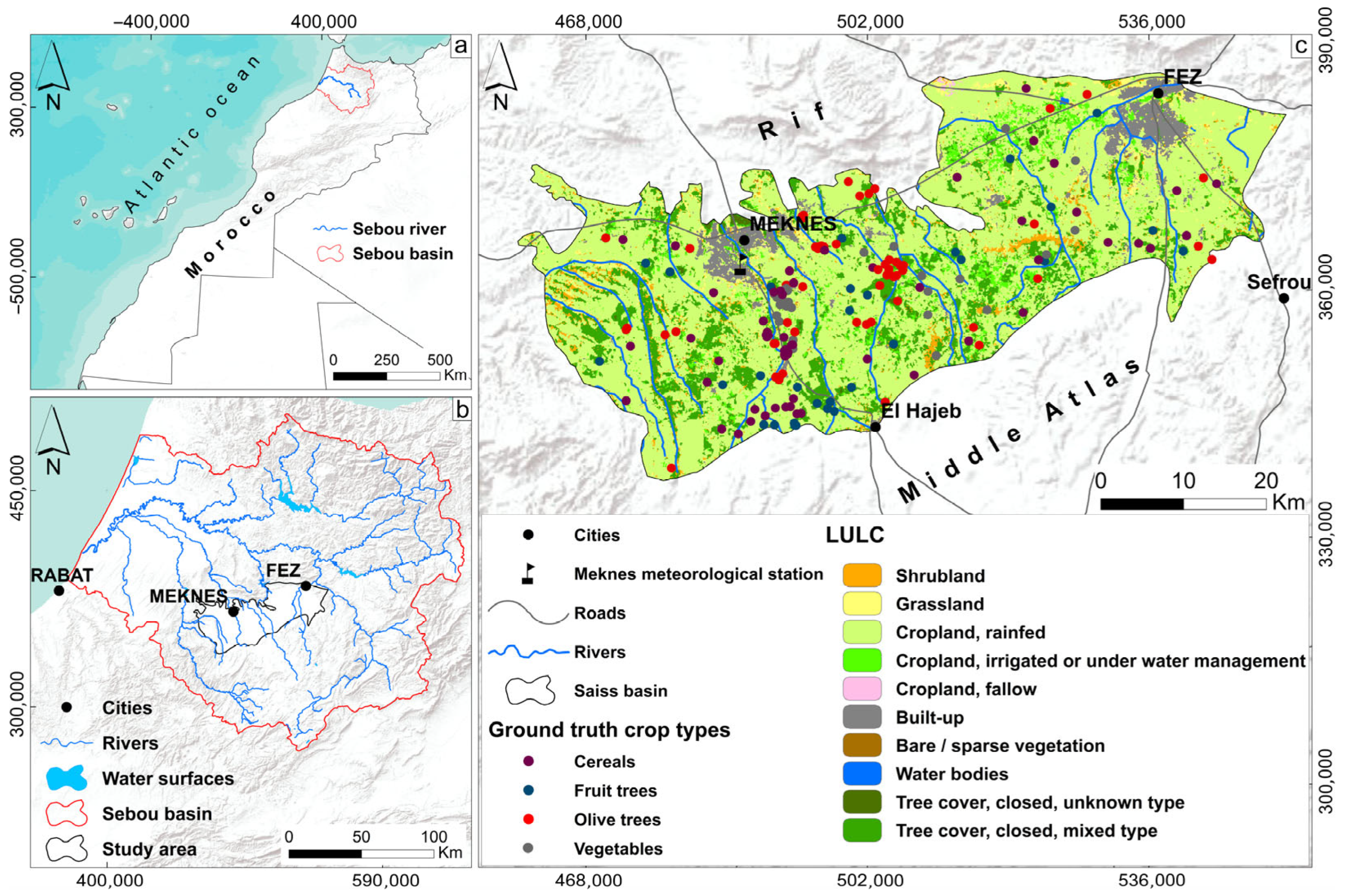
2.1. Study Area

This study was conducted in the Saiss plain (Figure 1), which is located in the Fez–Meknes region in northern Morocco (area ≈ 2300 km²), between latitudes 33°38′N and 34°4′N and longitudes 5°49′W and 4°53′W. Topographically, the study area is generally flat, with altitudes ranging from 212 m in the northeast to 1066 m in the southeast. The area is characterized by a semi-arid climate with dry and hot summers. Regarding rainfall, the inter-annual average for Meknes city has shown a negative trend, with 559 mm between 1934 and 2001 [50], 500 mm between 1998 and 2018 [49,51], and 300 mm between 2014 and 2023, according to the meteorological station of Meknes (Figure 2). Furthermore, the average annual temperature rose from 17.3 °C between 1934 and 2001 [50] to 17.6 °C between 1998 and 2018 [49,51,52] and 18.1 °C from 2014 to 2023, as reported by the Meknes meteorological station. According to the current climatic conditions in the Saiss plain between 2014 and 2023, two climatic periods make up the hydrological year: the wet period begins from the end of September until mid-May, characterized by the highest precipitation and lowest temperatures identified in January, known as the wet month. The dry period starts from mid-May until the end of September, with maximum temperatures and minimum precipitation recorded in August. The area is known for its high quality and abundance of water resources and fertile soils [53,54], enabling diversified agriculture (olive trees, fruit trees, cereals, vegetables, etc.) with a high level of efficiency. The agricultural sector is widely recognized as one of the main contributors to Morocco’s economy and society.

2.2. Data Collection

2.2.1. In Situ Measurements

The METRIC model requires local measurements of several weather variables, encompassing air temperature, precipitation, wind velocity, water vapor pressure, solar radiation, humidity, and reference ET (${ET}_r$). All these measurements were automatically recorded or calculated, in the case of ET, at 10-minute intervals by the Climatic Data Automatic Meteorological Station, equipped with the Campbell Scientific CR1000, situated at the Faculty of Sciences in Meknes (latitude: 33°52′11.12″N and longitude: 5°32′35.04″W). These data were used for the application, calibration, and testing of the METRIC model. To determine the ET for the main crops most commonly grown in the Saiss plain, it was necessary to collect verification points for each crop type (olive trees, fruit trees, cereals, and vegetables) in the study area (Figure 1c). Field missions were conducted during the specified period, and additional points were collected using satellite images from Google Earth during the study period.

2.2.2. MOD16 Products

The MODIS sensors onboard the Terra satellite provide MOD16A2 products. This is a global dataset of terrestrial ecosystem ET across vegetated areas [55]. Mu et al. [56,57] developed and subsequently improved the MOD16A2 ET algorithm based on the logic of the Penman–Monteith equation [2] and taking into account saturated vapor pressure and temperature. The improved algorithm refines the estimation of ET by first considering daytime fluxes and then incorporating calculations for both daytime and nighttime ET, streamlining the representation of the vegetation fraction, integrating the soil heat flux, estimating stomatal conductance, distinguishing between dry and wet canopy surfaces, and subdividing the soil surface into saturated wet and moisture surfaces. Hereafter, MOD16A2 products will be referred to as MODIS. MODIS has a spatial resolution of 500 m and a temporal resolution of 8 days and provides ET, potential ET, latent heat flux (LE), and potential LE, as well as the quality control (QC) data field. The MODIS ET is the sum of 8 days. Using the Google Earth Engine (GEE) computing platform, MODIS products available between September 2021 and August 2022 were processed to produce ET from vegetated areas. During this period, 46 ET maps were available (

Table 1. Dates of available MODIS products for September 2021–August 2022.

Image No.	Date	Measured ET (mm/day)	Image No.	Date	ETr (mm/day)
1	6 September 2021	3.2	24	6 March 2022	1.8
2	14 September 2021	2.6	25	14 March 2022	1.8
3	22 September 2021	3.0	26	22 March 2022	1.5
4	30 September 2021	2.7	27	30 March 2022	1.8
5	8 October 2021	2.3	28	7 April 2022	2.2
6	16 October 2021	1.9	39	5 April 2022	2.6
7	24 October 2021	1.7	30	23 April 2022	3.3
8	1 November 2021	1.5	31	1 May 2022	2.7
9	9 November 2021	1.0	32	9 May 2022	3.1
10	17 November 2021	1.2	33	17 May 2022	4.4
11	25 November 2021	0.8	34	25 May 2022	4.6
12	3 December 2021	0.8	35	2 June 2022	4.2
13	11 December 2021	1.0	36	10 June 2022	3.9
14	19 December 2021	1.1	37	18 June 2022	4.6
15	27 December 2021	0.9	38	26 June 2022	4.3
16	1 January 2022	1.3	39	4 July 2022	4.5
17	9 January 2022	1.0	40	12 July 2022	4.4
18	17 January 2022	1.3	41	20 July 2022	5.1
19	25 January 2022	1.2	42	28 July 2022	4.7
20	2 February 2022	1.5	43	5 August 2022	4.7
21	10 February 2022	1.6	44	13 August 2022	4.2
22	18 February 2022	1.6	45	21 August 2022	3.5
23	26 February 2022	1.8	46	29 August 2022	3.6

). They were subsequently downscaled and used to extract ET for each sampled crop type. Unfortunately, the accuracy test comparing MODIS-derived ET and the reference station’s ET could not be conducted because the climate station is located in an urban area where MODIS never provides ET values [55].

2.2.3. Landsat 8

This part of the study estimated the daily ET in the Saiss plain by applying the METRIC model using the Operational Land Imager (OLI) sensor and Thermal Infrared Sensor (TIRS) from the Landsat 8 satellite. The study area was located at the intersection of two satellite images (Path 201/Row 36 and Path 201/Row 37), necessitating the download of 24 images and subsequent mosaicking between each pair to obtain a total of 12 images covering the whole crop year (

Table 2. Availability of Landsat 8 images during the study period.

Image No.	Date	Time of Acquisition (hh:mm:ss) [UTC + 1]	ETr (mm/hr)
1	9 September 2021	10:57:42	0.33
2	27 October 2021	10:57:52	0.25
3	12 November 2021	10:57:48	0.18
4	30 December 2021	10:58:05	0.14
5	15 January 2022	10:57:39	0.13
6	16 February 2022	10:57:30	0.18
7	20 March 2022	10:57:18	0.28
8	21 April 2022	10:57:15	0.28
9	23 May 2022	10:57:22	0.44
10	8 June 2022	10:57:32	0.48
11	26 July 2022	10:57:48	0.49
12	11 August 2022	10:57:56	0.36

), provided that the images were clear and free from cloud cover. Images were available at least once a month between September 2021 and August 2022 and were acquired from the United States Geological Survey (USGS) (EarthExplorer (usgs.gov) (last accessed on 15 September 2022)). The METRIC model inputs were calculated for the time of the satellite overpass using multispectral bands (bands 2, 3, 4, 5, 6, and 7) for albedo (α) and vegetation index calculation (Soil Adjusted Vegetation Index (SAVI) and Leaf Area Index (LAI)). In addition, thermal bands (bands 10 and 11) were used to produce the land surface temperature (LST) and surface emissivity. The spatial resolution was enhanced to 15 m × 15 m for all the bands using the panchromatic band (band 8). These and other input variables were used, after the necessary corrections and treatments, to solve the SEB equation.

2.3. METRIC Model

The METRIC model is a complex algorithm for calculating ET as a residual of the surface energy balance. Its general equation is as follows [25,26]:

LE = Rₙ − G − H

(1)

where LE is the latent heat flux (W/m²) associated with the phase change of water from liquid to vapor during evapotranspiration; Rₙ is the net radiation flux density at the surface (W/m²); G is the ground heat flux density (W/m²), representing the sensible heat conducted into the soil; and H is the sensible heat flux density (W/m²) transferred to the atmosphere through convection.

2.3.1. Net Radiation Flux (Rₙ)

The net radiation (Rₙ) is the algebraic sum of different forms of radiative exchange. The R_n flux is calculated from the ground radiation flux balance.

$$R_n=\left(1-\alpha \right)R_s\downarrow +R_l\downarrow -R_l\uparrow -(1-{\epsilon }_g)R_l\downarrow$$

(2)

where $\alpha$ is the surface albedo; $R_s\downarrow$ is the incoming shortwave radiation (W/m²); $R_l\downarrow$ is the incoming longwave radiation (W/m²); $R_l\uparrow$ is the outgoing longwave radiation (W/m²); and ${\epsilon }_g$ is the land surface emissivity.

The surface albedo is a measure of how effectively a surface reflects solar radiation, according to the following formula [58]:

$$\alpha ={\rho }_0+{\sum }_{i=1}^n{\rho }_i{w}_i$$

(3)

where $n$ is the number of spectral bands used (specifically, $n=7$); ${\rho }_0$ is the intercept with a value of −0.0015; $w_i$ denotes the weighting coefficients with respective values of 0.160, 0.291, 0.243, 0.116, 0.112, 0, and 0.081 [59]; and ${\rho }_i$ denotes the reflectance values across the 12 Landsat bands.

The incoming shortwave radiation ${(R}_s\downarrow$), incoming longwave radiation $(R_l\downarrow )$, and outgoing longwave radiation ${(R}_l\uparrow$) were calculated as follows [19,60]:

$$Rₛ\downarrow =G_{SC}cos\theta d_r{\tau }_{sw}$$

(4)

$$R_l\downarrow ={\epsilon }_a\sigma T_a^4$$

(5)

$$R_l\uparrow ={\epsilon }_g\sigma T_s^4$$

(6)

where $G_{SC}$ is the solar constant (1367 W/m²); $d_r$ is the inverse square of the relative Sun–Earth distance; $cos\theta$ denotes the cosine of the solar zenith angle; $\sigma$ is the Stefan–Boltzmann constant (measured at 5.67 × 10⁻⁸ W/(m²·K⁴)); ${\tau }_{sw}$ is the atmospheric transmissivity; ${\epsilon }_a$ is the atmospheric emissivity; and $T_a$ and $T_s$ refer to the air and land surface temperatures (K).

2.3.2. Soil Heat Flux ($G$)

The soil heat flux refers to the rate at which heat is accumulated in the soil and vegetation by conduction. The computation of G uses an empirical equation developed by Bastiaanssen et al. [61], which provides values approximating those observed around midday.

$$G={\left(T_s-273.15\right)(0.0038+0.0074\alpha )(1-0.98NDVI}^4)R_n$$

(7)

2.3.3. Sensible Heat Flux Density ($H$)

The calculation of $H$ is the most challenging task, as it plays a critical role in characterizing the energy exchange between the land surface and the atmosphere. The H function is customized for each individual satellite image. $H$ is derived from an aerodynamic function, determined as follows [61]:

$$H={{\rho }_{air}C}_p{\displaystyle \frac{dT}{r_{ah}}}$$

(8)

where ${\rho }_{air}$ is the air density (kg/m³); $C_p$ is the specific heat capacity of air at constant pressure (J/(kg·K)); $dT$ is the temperature difference (K); and $r_{ah}$ is the aerodynamic resistance to heat transfer between two near-surface heights (s/m).

For neutral stability, $r_{ah}$ is calculated as follows:

$$r_{ah}={\displaystyle \frac{\mathit{ln}\left(\frac{z_2}{z_1}\right)}{U_f\ast k}}$$

(9)

where $z_1$ and $z_2$ are heights (in meters) measured above the zero-plane displacement of the vegetation, with values of 2.0 m and 0.1 m, respectively. $U_f$ represents the friction velocity (m/s), and $k$ is the Von Karman constant, typically set at 0.41.

$$U_f={\displaystyle \frac{k{u}_{200}}{\mathit{ln}\left(\frac{200}{z_{om}}\right)}}$$

(10)

where $u_{200}$ is the wind speed (m/s) at a standard blending height of 200 m, while $z_{om}$ is the momentum roughness length (m), which is calculated for each pixel by the Leaf Area Index (LAI) (dimensionless) as follows [62]:

$$z_{om}=0.018\times LAI$$

(11)

To calculate $H$ from Equation (8), the near-surface vertical air temperature difference (dT) must be determined for each pixel. This temperature difference is defined at heights $z_1$ and $z_2$ for each pixel as follows:

$$dT={Tz}_1-{Tz}_2$$

(12)

where ${Tz}_1$ and ${Tz}_2$ are the air temperatures at $z_1$ and $z_2$, respectively. While the absolute values of ${Tz}_1$ and ${Tz}_2$, and the air temperature above each pixel are not directly known, $dT$ is required to estimate H. This difference has been shown to correlate strongly with the radiometric surface temperature ($T_s$) [25,26]. Consequently, the METRIC model assumes a linear relationship between $dT$ and $T_s$, which is calibrated to each satellite image to derive $dT$ at the pixel level [31]:

$${dT=b+aT}_s$$

(13)

where $b$ and $a$ are the calibration coefficients determined involves the CIMEC (Calibration Using Inverse Modeling at Extreme Conditions) approach, which enhances the accuracy of the METRIC model. Hot pixels are typically located in sparsely vegetated or bare soil areas, where latent heat flux (LE) is minimal and the sensible heat flux ($H$) approximates the difference between $R_n$ and $G$. Conversely, cold pixels are chosen from densely vegetated, moist areas, where LE dominates and closely matches $R_n-G$, resulting in minimal $H$. Pixel selection is guided by LST and NDVI [63]. Atmospheric stability is a critical factor in this process, as it significantly affects aerodynamic resistance, particularly under dry conditions. To account for this, the METRIC model incorporates the Monin–Obukhov similarity theory in an iterative framework, ensuring stable and accurate estimates of $H$ and aerodynamic resistance. Further details on the iterative process can be found in [25,26].

2.3.4. Daily ET

Derived from the surface energy balance (Equation (1)), LE is computed as the residual. For each pixel, LE was calculated as ET at the time of the exact satellite overpass using Equation (14). The energy balance approach offers the advantage of computing actual ET, rather than potential ET, making it more responsive to vegetation conditions and capable of detecting reductions in ET due to soil moisture deficits. However, the accuracy of the latent heat flux (LE) calculation depends on the accuracy of the individual components, i.e., $R_n$, $G$, and $H$. The METRIC model addresses this uncertainty by internally calibrating $H$, which compensates for intermediate estimation errors and biases. Studies such as [41] have shown that the METRIC model is less sensitive to the absolute accuracy of Landsat-derived surface temperature. To calculate ET at the satellite image overpass time, the LE value from Equation (1) is divided by the latent heat of vaporization:

$${ET}_{inst}=3600\times {\displaystyle \frac{LE}{\lambda {\rho }_w}}$$

(14)

where ${ET}_{inst}$ is the instantaneous ET rate (mm · h⁻¹); the factor 3600 converts seconds to hours; ${\rho }_w$ is the density of water (~1000 Kg · m⁻³); and $\lambda$ is the latent heat of vaporization (denoting the heat required to evaporate one kilogram of water) and is calculated as follows [25,26]:

$$\lambda =\left[2.501-0.00236(T_s-273)\right]\times {10}^6$$

(15)

The ET reference fraction $\left({ET}_{r}F\right)$ for individual pixels was used to estimate or extend actual ET over time through interpolation or extrapolation. ${ET}_{r}F$ was determined by dividing the calculated instantaneous ET (${ET}_{inst}$) of each pixel by the reference ET (${ET}_r)$, derived from weather data. Only one or two meteorological stations are needed to estimate ${ET}_r$ in the manual METRIC process for a Landsat image [25]. This method uses weather-derived ${ET}_r$ to capture hourly or daily ET variations due to weather changes. ${ET}_{r}F$ reflects the influence of vegetation cover and water availability on the ET process. By interpolating ${ET}_{r}F$ across satellite overpass dates and multiplying it by daily ${ET}_r$, daily actual ET $\left({ET}_a\right)$ can be derived.

$${ET}_{r}F={ET}_{inst}/{ET}_r$$

(16)

The daily actual evapotranspiration (${ET}_a$ or ${ET}_{24}$) for each pixel was calculated using Equation (17).

$${ET}_{24}={ET}_{r}F\ast {ET}_{r24}$$

(17)

where ${ET}_{r24}$ is the daily reference ET (mm · day⁻¹), and ${ET}_{24}$ is the daily ${ET}_a$ (mm · day⁻¹).

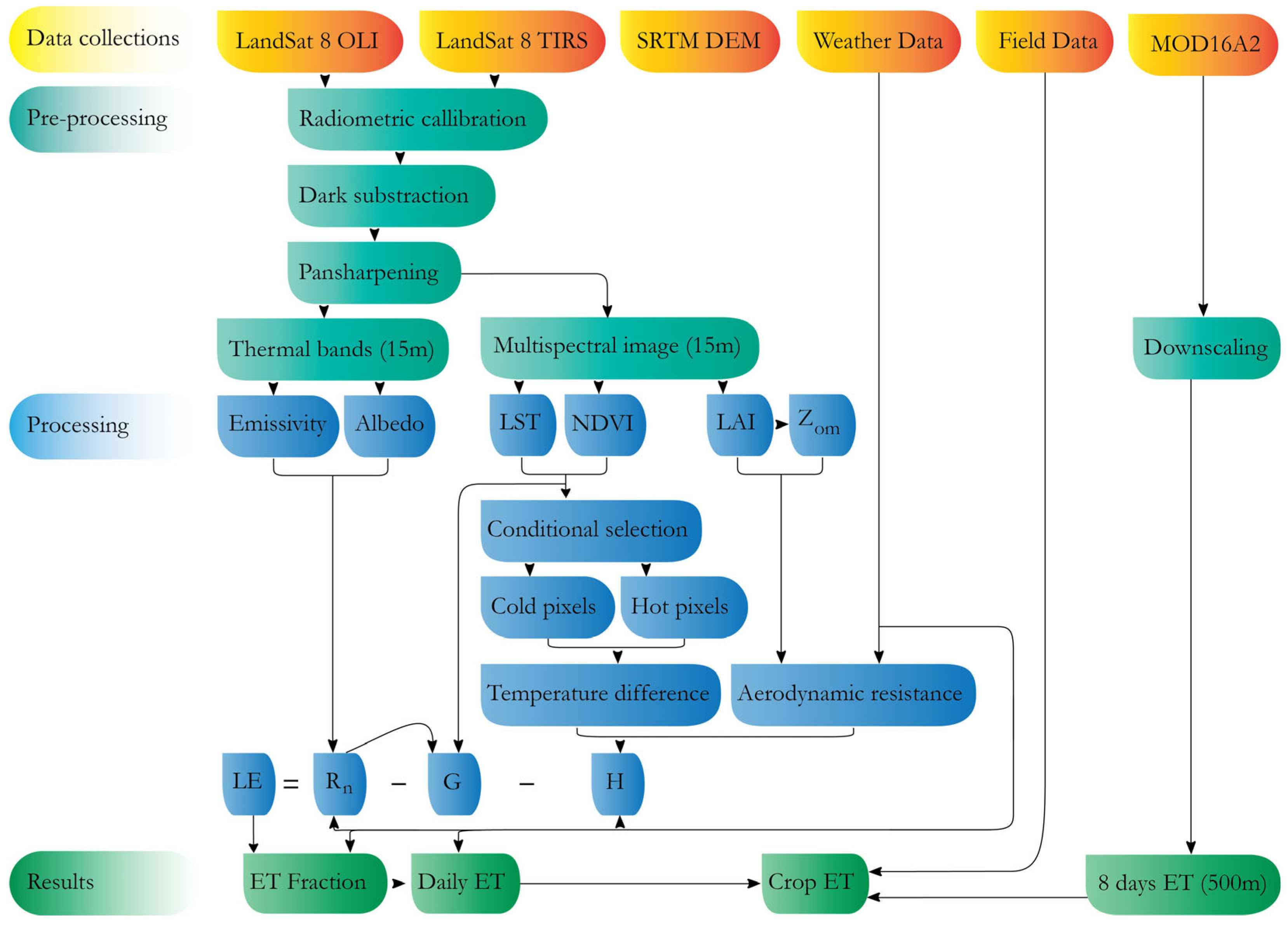
2.4. Technical Processing

The methodological workflow for estimating ET using remote sensing imagery, the METRIC model, and the MODIS product processing is summarized in Figure 3.

2.5. Evaluation and Validation

The ET derived from the MODIS global products with a resolution of 500 m was compared with the ET derived from the METRIC model. The purpose of this comparison was to test the feasibility of the METRIC model to capture ET. Since the MODIS products were sums taken over a period of eight days, the METRIC model results were converted to the 8-day intervals for comparison. The following equation was applied [64]:

$${ET}_{8d}={ET}_d\ast \left({\displaystyle \frac{{ET}_{0-8d}}{{ET}_{0-d}}}\right)$$

(18)

where ${ET}_d$ is the resulting daily METRIC ET, and ${ET}_{0-8d}$ and ${ET}_{0-d}$ are the 8-day reference ET and daily reference ET, respectively, which were collected from the reference ET.

The METRIC model results were evaluated against observed reference ET series. The METRIC model performance was evaluated by the coefficient of determination (R², Equation (19)), root mean square error (RMSE, Equation (20)), mean absolute error (MAE, Equation (21)), and by graphical plots between the simulated and observed data.

$$R^2={\displaystyle \frac{\sum _{i=1}^n({ET}_o-\overline{{ET}_o})({ET}_s-\overline{{ET}_s})}{\sqrt{{\sum _{i=1}^n({ET}_o-\overline{{ET}_o})}^2}\sum _{i=1}^n{({ET}_s-\overline{{ET}_s})}^2}}$$

(19)

$$\mathrm{R}\mathrm{M}\mathrm{S}E=\sqrt{{\displaystyle \frac{1}{n}}\sum _{i=1}^n{({ET}_O-{ET}_s)}^2}$$

(20)

$$\mathrm{M}\mathrm{A}E={\displaystyle \frac{1}{n}}\sum _{i=1}^n\left|{ET}_O-{ET}_s\right|$$

(21)

where ${ET}_0$ is the reference ET value; ${ET}_s$ is the simulated ET value; ${ET}_0$ is the mean of observations; ${ET}_s$ is the mean of simulations; and n is the number of time intervals.

The NSE varies between −∞ and 1, with a value of 1 indicating that the simulated data are equal to the observed data. R² ranges from 0 to 1. A value of 0 indicates that there is no correlation between the two time series, while a value of 1 indicates a very strong linear correlation. Unlike the Nash–Sutcliffe criteria, when the coefficient of determination is close to 1, it does not indicate that the observed and simulated series are similar, but that they are proportionally related.

3. Results

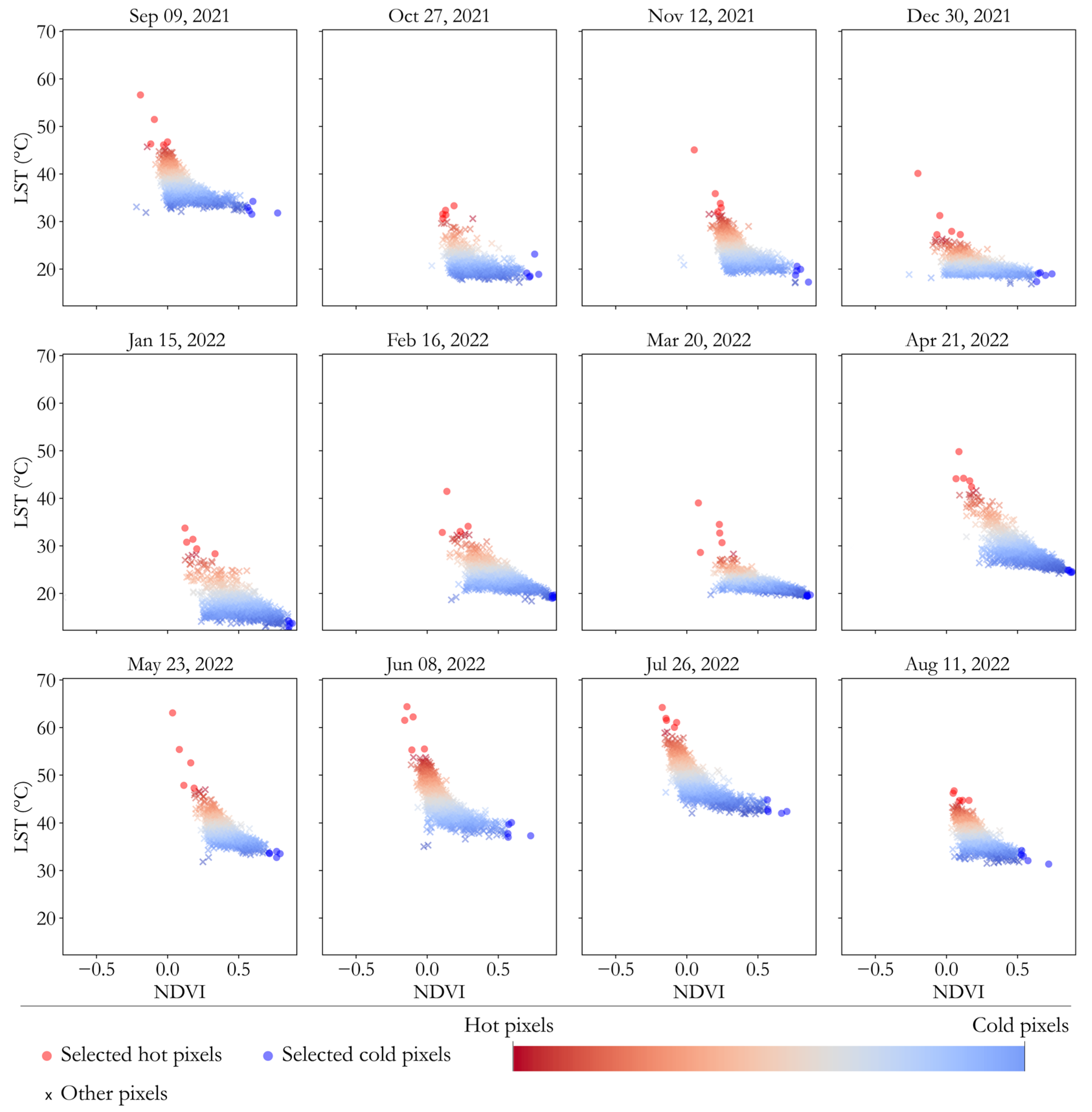
3.1. NDVI and LST Dynamics

Land surface temperature (LST), calculated from Landsat 8 satellite thermal bands, and the Normalized Difference Vegetation Index (NDVI), calculated from the same satellite’s OLI sensor, were key inputs for ET estimation via the SEB equation. The correlation between NDVI and LST for the different LULC classes in the study area was established. For all processed images, NDVI ranged from an average minimum value of −0.45 to an average maximum value of 0.81. The surface temperature varied between an average minimum of 24.4 °C and an average maximum of 51.3 °C (Figure 4). This correlation was used to define cold and hot pixels used to calibrate H. The blue points in the graphs represent the selected cold pixels, while the red points represent the hot pixels. The NDVI-LST scatterplot showed expected trends: densely vegetated areas (high NDVI) corresponded to lower LSTs due to evaporative cooling, while arid regions (low NDVI) showed elevated LSTs.

3.2. Spatiotemporal Variation of ET

The spatiotemporal results of daily ET were obtained by applying the METRIC model to satellite images from Landsat 8 with a spatial resolution of 15 m, alongside meteorological data from the local weather station. During the 2021–2022 hydrological year, ET estimates in the Saiss plain ranged from a minimum average of approximately 0.1 mm/day simulated in March 2022 to a maximum average of 11 mm/day simulated in July of the same year. Spatially, the lowest ET rates were primarily simulated in urbanized areas, notably the cities of Meknes and Fez, followed by bare soils. The highest values were simulated in intensively cultivated areas. Seasonal trends were evident, with average ET values ranging from 2.3 mm/day in January to 9.4 mm/day in July, reflecting increased crop water use during the growing season (Figure 5).

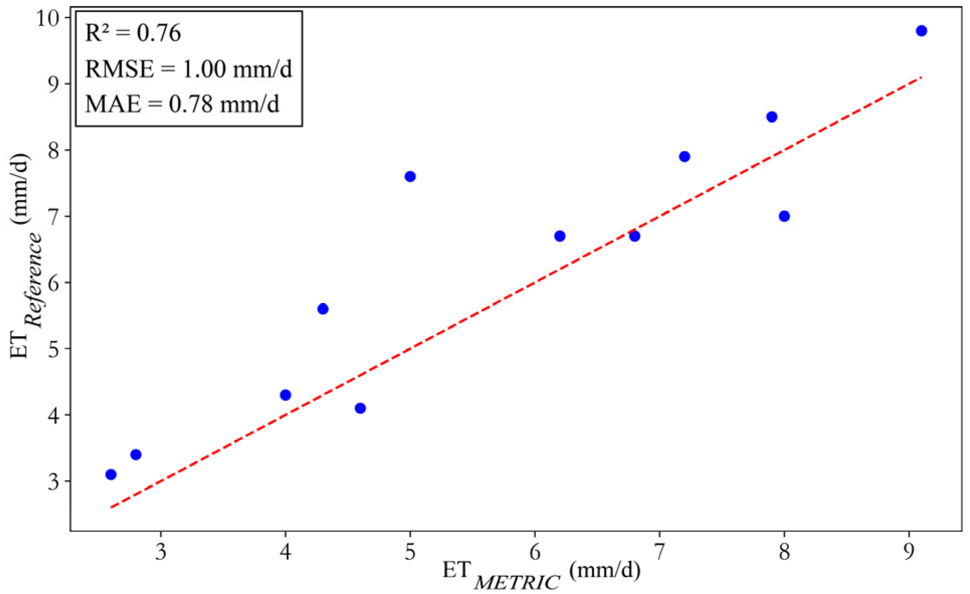
3.3. Comparison Between Measured and Modeled ET

The accuracy of the METRIC model was evaluated by comparing the reference ET observations with simulated ET values extracted at the pixel corresponding to the Meknes meteorological station on each date (Figure 6). The reference ET corresponded to the same day as the satellite overpass. Statistical analysis (Figure 6) revealed a strong agreement between modeled and reference ET, with an R² of 0.76, an RMSE of 1 mm/day, and an MAE of 0.78 mm/day.

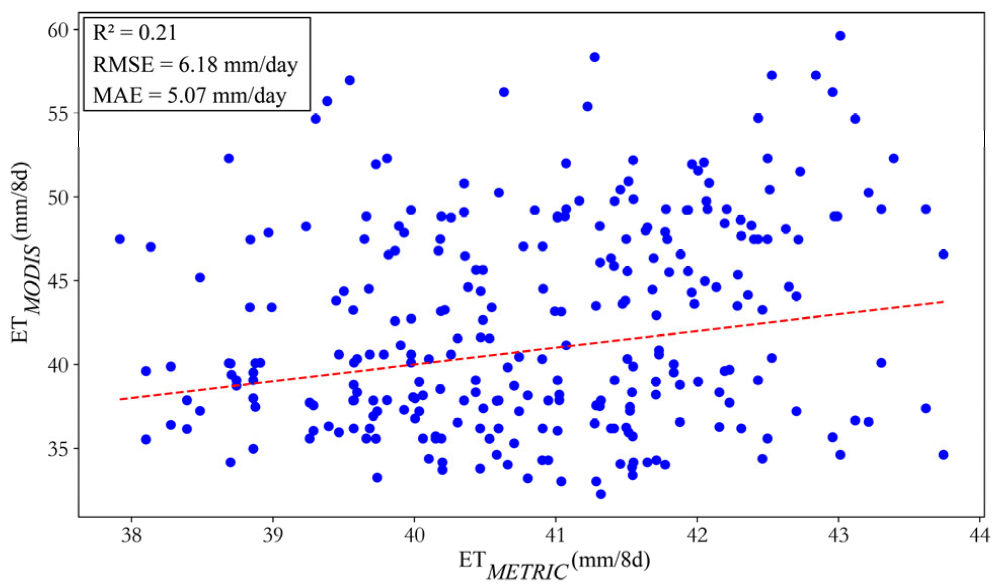
3.4. Comparison of METRIC ET and MODIS ET

To validate the performance, METRIC-derived ET values were compared with MODIS-derived ET for the same period (September 2021 to August 2022). The performance analysis was based on ET values extracted from agricultural areas. These points were located entirely within the agricultural area, where MODIS provided ET estimates. The results (Figure 7) show a low agreement between METRIC and MODIS ET for the agricultural area, with a low R² (0.21) and relatively high RMSE (6.18 mm/day) and MAE (5.07 mm/day) values. Generally, MODIS provided estimates that were higher than those calculated by the METRIC model.

3.5. Crop ET

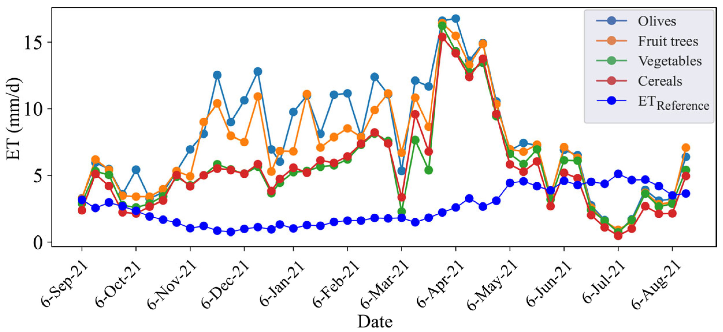
3.5.1. Crop ET Derived from the METRIC Model

Figure 8 illustrates the estimated ET for the main crop types cultivated in the Saiss plain (olives, fruit trees, vegetables, and cereals) during the study period, alongside the reference ET values for the corresponding dates. Temporal trends in ET were consistent across all crop types. The minimum estimated daily ET values were observed on 15 January 2022 (olives: 3.4 mm/day; fruit trees: 2.8 mm/day; vegetables: 2.6 mm/day; cereals: 2.3 mm/day). The maximum ET values occurred in July (olives: 10 mm/day; fruit trees: 9.6 mm/day; vegetables: 8.8 mm/day; cereals: 8.4 mm/day). Across all crop types, crop ET values consistently exceeded the reference ET on all observation dates. ET variability reflected seasonal climatic conditions, with lower rates during wet periods and higher rates during dry periods. Olive trees exhibited the highest ET values among crop types, followed by fruit trees, vegetables, and cereals, highlighting the different water use of agricultural crops in the Saiss plain. The July peaks coincided with peak growing-season water use and elevated temperatures, while the January minima coincided with reduced solar radiation and dormant phases.

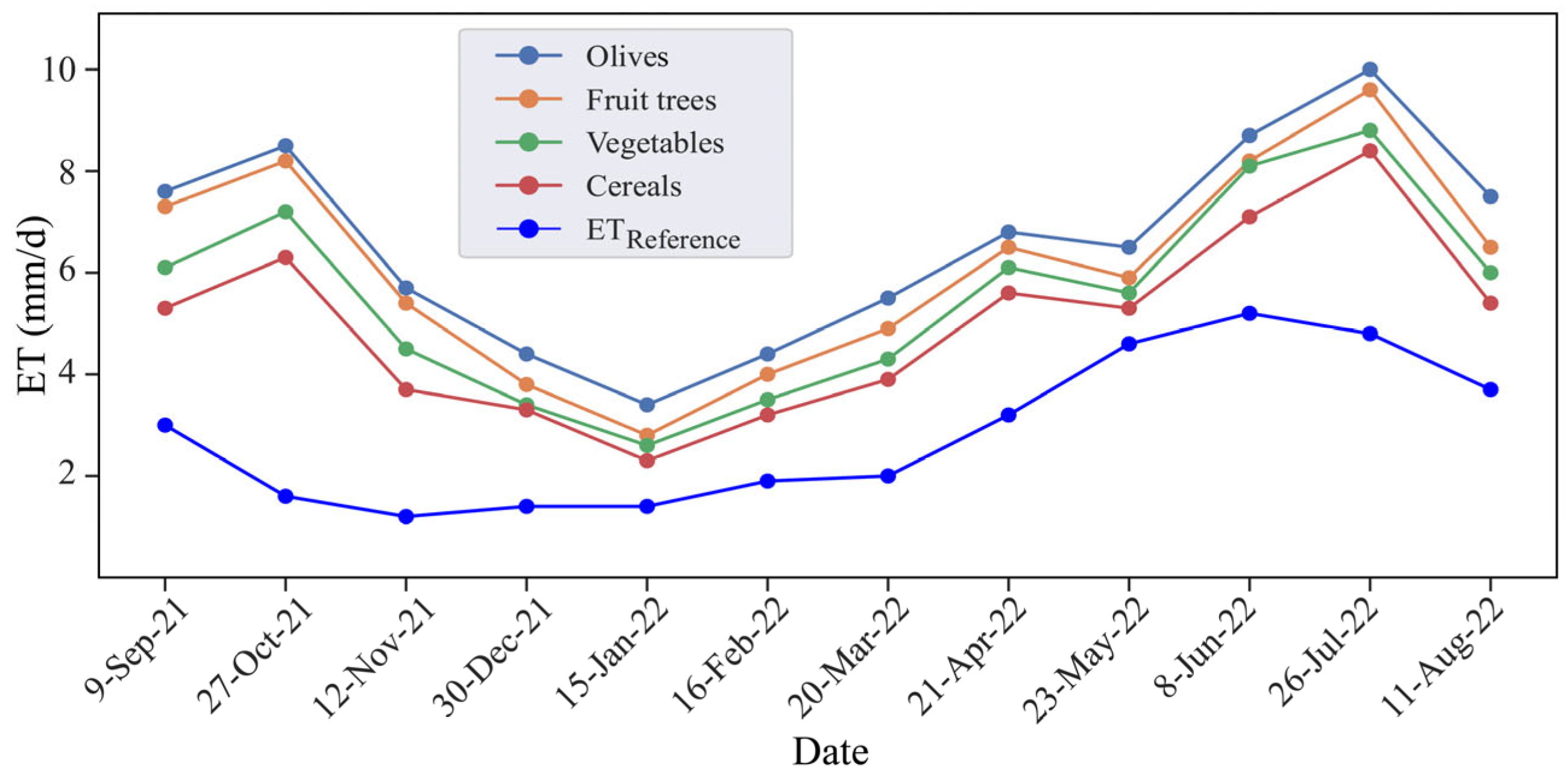
3.5.2. Crop ET Derived MODIS

Using the GEE platform, ET for the four major crop types was generated at a 500 m resolution (Figure 9). The processing involved downscaling and extracting ET at multiple locations of the four sampled crop types in the Saiss plain. However, MODIS ET was restricted to green areas with vegetation and excluded urban areas. This made it impossible to correlate MODIS ET with reference ET, since the station is located in the city of Meknes. The temporal patterns of MODIS-derived ET for the various crop types exhibited consistent seasonal trends but varied in magnitude across crop types. The MODIS ET curves were different from the reference ET curve. Minimum daily MODIS ET values occurred in July (olives: 7.1 mm/day; fruit trees: 9.1 mm/day; vegetables: 7.3 mm/day; cereals: 5.4 mm/day), while maximum MODIS ET values were observed in April (olives: 16.6 mm/day; fruit trees: 16.4 mm/day; vegetables: 16.2 mm/day; cereals: 15.4 mm/day). Unlike the reference ET, the MODIS estimates were higher during wet periods and lower during dry periods, with a considerable underestimation during the hot season. This discrepancy suggests that MODIS may underestimate crop water stress during peak drought conditions.

4. Discussion

The accuracy of sensible heat fluxes relied heavily on the precise calibration of selected extreme pixels, which reflected the specific land surface conditions of the study area. The calibration was based on the analysis of LULC classes and their corresponding LST and NDVI values. These indices were crucial for the identification of ‘cold’ and ‘hot’ pixels, which represented the extremes of moisture conditions within the region. Particularly, ‘cold’ pixels corresponded to zones with areas of high NDVI values (NDVI > 0.6) and low LST, indicating moist, vegetated areas with robust transpiration and consequently higher ET. Conversely, ‘hot’ pixels were characterized by low or absent NDVI (NDVI < 0.2) and high LST, consistent with arid, unvegetated areas where ET was minimal or absent. These findings have been corroborated in a number of locations [43,65,66,67,68]. The selection of suitable cold and hot pixel thresholds is crucial, as it provides the basis for the model’s energy balance calculations and significantly influences sensible heat flux estimations [20,25]. By establishing these key reference points, the METRIC model was able to quantify the heat transferred to the atmosphere more accurately under varying degrees of surface wetness. This led to a more nuanced and accurate representation of ET across different LULC classes.

The synergistic use of spatial remote sensing, climate data, and field data has enabled the spatiotemporal monitoring of ET on a regional scale. However, the accuracy of the estimation results remains a major challenge [29,63]. The monitoring of ET across the agriculturally heterogeneous Saiss plain was carried out for the first time using an SEB model and MODIS products due to the availability of satellite imagery and meteorological station data. The heterogeneous land cover of the Saiss plain, which is predominantly agricultural, required the METRIC model to be adapted to estimate ET during the 2021–2022 hydrological year. The validation of the estimation results was made possible by the availability of reference ET data from the Meknes meteorological station. Unfortunately, MODIS ET could not be validated locally with reference ET due to the lack of ET estimates around the meteorological station [55]. The METRIC model was first validated using reference ET and then compared with MODIS. METRIC estimates agreed well with reference ET, as evidenced by the statistical metrics of model performance (R², RMSE, and MAE). However, the same metrics showed a low level of agreement between MODIS ET and METRIC ET. This statistical analysis indicated that METRIC’s estimates were superior in the Saiss plain, with acceptable errors.

The low agreement between METRIC and MODIS ET estimates was attributed to several factors. A primary contributor is the significant difference in spatial resolution: METRIC provides ET estimates at a much finer resolution (15 m) compared to MODIS, which operates at a coarser resolution (500 m). This disparity can lead to mixed pixel effects in MODIS data, especially in heterogeneous agricultural landscapes such as the Saiss plain, resulting in overestimations in certain areas. Furthermore, the heterogeneity of land features, such as varying crop types, crop conditions, and land management practices, affects the accuracy of satellite-based ET estimates, and MODIS algorithms may not fully capture this local variability. Differences in retrieval algorithms also play a role: METRIC is a physics-based model using surface temperature and reflectance data, while MODIS ET products rely on different empirical assumptions and physical principles. Additionally, variations in the timing of satellite overpasses and data acquisition dates may influence the comparability of the datasets, with mismatched temporal snapshots further contributing to the observed differences. Collectively, these factors explain the low R² and high error values, highlighting the need for multi-source approaches and careful consideration of each method’s limitations when estimating ET in complex, diverse landscapes.

The accuracy of the METRIC model stems from its physical basis in the surface energy balance (SEB) equation, its calibration using local extreme pixels, and the high resolution of the Landsat thermal bands, which enable precise delineation of field-scale variability [9,41]. The model included the various variables related to ET, namely LST, NDVI, temperature, wind speed, and radiation. The high resolution of the Landsat images used (15 m) allowed clear identification of the LULC types, leading to more accurate estimates. While MODIS provides continuous global ET estimates, its coarse resolution (500 m) resulted in overestimation of ET in the study area, primarily due to its inability to resolve fine-scale land cover variations or incorporate local calibration. As a global product, MODIS ET does not account for local conditions and could not be validated locally due to the absence of flux tower observations needed to calibrate the parameters of the ET algorithm [69]. This further highlights the advantage of METRIC for regional studies requiring site-specific adjustments.

From September 2021 to August 2022, the temperature evolution was anomalously high among the four dominant crop types in the Saiss plain. The impact on the daily ET of the crop types was as follows: olives > fruit trees > vegetables > cereals. This hierarchy closely mirrors the findings of [49], who quantified the water demand of these same crop types in another part of the Saiss plain. Crop types that consumed more water had higher ET rates. ET is mainly controlled by temperature, which determines the atmospheric demand for water and the availability of water to meet this demand. In the study area, temperatures were higher than usual, especially during 2021–2022 [51], while precipitation had declined significantly. Olives, fruit trees, and vegetables are generally irrigated and had the highest ET rates. Cereals are the most abundant crop in the Saiss plain, the country’s principal production area, but they rely on rainfall and are not irrigated; consequently, cereals exhibited the lowest ET rates.

One limitation of this study is that the METRIC model was validated using ET data from the urban weather station in Meknes, which may not fully represent agricultural microclimates. Due to the lack of ET measurements in farmland areas, this dataset was the only one available. This highlights the importance of conducting more field-based observations in rural areas to support future calibration and validation efforts.

5. Conclusions

This study presents the first high-resolution estimation and assessment of evapotranspiration in Morocco’s agriculturally important Saiss plain during the drought year from September 2021 to August 2022, using the METRIC model applied to Landsat 8 satellite imagery. The results provide valuable insights into the spatiotemporal dynamics of ET across four different crop types. Validation of the METRIC model against reference ET values, obtained from a local meteorological station, showed strong performance, with an R² of 0.76, an RMSE of 1 mm/day, and an MAE of 0.78 mm/day. These results confirm the robust reliability of the METRIC model for estimating ET in the Saiss plain within an acceptable margin of error. The high spatial resolution of Landsat 8 images enabled the model to capture high spatial resolution variations in ET, which is essential for accurate water balance assessments in this heterogeneous agricultural region. When comparing METRIC ET estimates with MODIS-derived ET, a low agreement was observed (R² = 0.21, RMSE = 6.18 mm/day, MAE = 5.07 mm/day). MODIS tends to estimate different ET values, likely due to its coarse spatial resolution (500 m) and the generalized algorithms, both of which may result in an inaccurate representation of local conditions. This discrepancy highlights the importance of selecting appropriate satellite products and models that align with the specific requirements and spatial scale of the local conditions. Spatiotemporal ET estimates from the METRIC model revealed considerable variation in ET rates across different LULC classes during the 2021–2022 hydrological year. ET rates ranged from a minimum of approximately 0.1 mm/day in March 2022 to a maximum of 9.4 mm/day in July. Urban areas, such as Meknes and Fez, exhibited the lowest ET rates, while cultivated irrigated areas displayed the highest rates. These findings underscore the important role of vegetation cover and land use in influencing ET rates and patterns. The ability to map these variations with a high spatial resolution of 15 m provides valuable insights for the management of water resources in the Saiss plain. The temporal evolution of ET for four different crop types revealed distinct patterns. Olive trees exhibited the highest ET rates, followed by fruit trees, vegetables, and cereals. This hierarchy is consistent with the findings of previous studies on the water requirements of these crop types in the Saiss plain. ET rates were highest during dry periods, particularly in July, and lowest during wet periods. These results underscore the important influence of irrigation and crop type on ET dynamics. Olives, fruit trees, and vegetables are usually irrigated, whereas cereals mainly rely on rainfall, which affects their ET rates. The ability to accurately estimate and monitor ET at high spatial and temporal resolutions is essential for effective water resource management, particularly in agricultural regions such as the Saiss plain. The METRIC model, which has been validated against local reference ET data, provides reliable ET estimates that can contribute to irrigation scheduling, drought management, and overall water resource planning. Discrepancies between METRIC and MODIS ET estimates also highlight the importance of careful consideration of satellite product selection based on study objectives and spatial resolution requirements.

References

1. Zhang, K.; Kimball, J.S.; Running, S.W. A review of remote sensing based actual evapotranspiration estimation. WIREs Water 2016, 3, 834–853. [Google Scholar] [CrossRef]
2. Allen, R.G.; Pereira, L.S.; Raes, D.; Smith, M. Crop Evapotranspiration-Guidelines for Computing Crop Water Requirements-FAO Irrigation and Drainage Paper 56; FAO: Rome, Italy, 1998; Volume 300, p. D05109. [Google Scholar]
3. Allen, R.G.; Morse, A.; Tasumi, M.; Bastiaanssen, W.; Kramber, W.; Anderson, H. Evapotranspiration from Landsat (SEBAL) for water rights management and compliance with multi-state water compacts. In Proceedings of the IGARSS 2001. Scanning the Present and Resolving the Future. Proceedings. IEEE 2001 International Geoscience and Remote Sensing Symposium (Cat. No. 01CH37217), Sydney, NSW, Australia, 9–13 July 2001; Volume 2, pp. 830–833. [Google Scholar]
4. Allen, R.G.; Dhungel, R.; Dhungana, B.; Huntington, J.; Kilic, A.; Morton, C. Conditioning point and gridded weather data under aridity conditions for calculation of reference evapotranspiration. Agric. Water Manag. 2021, 245, 106531. [Google Scholar] [CrossRef]
5. Wang, L.; Wang, J.; Ding, J.; Li, X. Estimation and Spatiotemporal Evolution Analysis of Actual Evapotranspiration in Turpan and Hami Cities Based on Multi-Source Data. Remote Sens. 2023, 15, 2565. [Google Scholar] [CrossRef]
6. Allies, A. Estimation de L’évapotranspiration par Télédétection Spatiale en Afrique de l’Ouest: Vers une Meilleure Connaissance de Cette Variable clé Pour la Région. Ph.D. Thesis, Université Montpellier, Montpellier, France, 2018. [Google Scholar]
7. Allen, R.G.; Pereira, L.S.; Howell, T.A.; Jensen, M.E. Evapotranspiration information reporting: II. Recommended documentation. Agric. Water Manag. 2011, 98, 921–929. [Google Scholar] [CrossRef]
8. Dos Santos, R.A.; Mantovani, E.C.; Fernandes-Filho, E.I.; Filgueiras, R.; Lourenço, R.D.S.; Bufon, V.B.; Neale, C.M.U. Modeling Actual Evapotranspiration with MSI-Sentinel Images and Machine Learning Algorithms. Atmosphere 2022, 13, 1518. [Google Scholar] [CrossRef]
9. García-Santos, V.; Sánchez, J.M.; Cuxart, J. Evapotranspiration Acquired with Remote Sensing Thermal-Based Algorithms: A State-of-the-Art Review. Remote Sens. 2022, 14, 3440. [Google Scholar] [CrossRef]
10. Ghiat, I.; Mackey, H.R.; Al-Ansari, T. A Review of Evapotranspiration Measurement Models, Techniques and Methods for Open and Closed Agricultural Field Applications. Water 2021, 13, 2523. [Google Scholar] [CrossRef]
11. Wanniarachchi, S.; Sarukkalige, R. A Review on Evapotranspiration Estimation in Agricultural Water Management: Past, Present, and Future. Hydrology 2022, 9, 123. [Google Scholar] [CrossRef]
12. Derardja, B.; Khadra, R.; Abdelmoneim, A.A.A.; El-Shirbeny, M.A.; Valsamidis, T.; De Pasquale, V.; Deflorio, A.M.; Volden, E. Advancements in Remote Sensing for Evapotranspiration Estimation: A Comprehensive Review of Temperature-Based Models. Remote Sens. 2024, 16, 1927. [Google Scholar] [CrossRef]
13. Lakhiar, I.A.; Yan, H.; Zhang, C.; Zhang, J.; Wang, G.; Deng, S.; Syed, T.N.; Wang, B.; Zhou, R. A review of evapotranspiration estimation methods for climate-smart agriculture tools under a changing climate: Vulnerabilities, consequences, and implications. J. Water Clim. Chang. 2024, 16, 249–288. [Google Scholar] [CrossRef]
14. Karimi, P.; Bastiaanssen, W.G.M. Spatial evapotranspiration, rainfall and land use data in water accounting—Part 1: Review of the accuracy of the remote sensing data. Hydrol. Earth Syst. Sci. 2015, 19, 507–532. [Google Scholar] [CrossRef]
15. Jing, W.; Yaseen, Z.M.; Shahid, S.; Saggi, M.K.; Tao, H.; Kisi, O.; Salih, S.Q.; Al-Ansari, N.; Chau, K.-W. Implementation of evolutionary computing models for reference evapotranspiration modeling: Short review, assessment and possible future research directions. Eng. Appl. Comput. Fluid. Mech. 2019, 13, 811–823. [Google Scholar] [CrossRef]
16. Chen, J.M.; Liu, J. Evolution of evapotranspiration models using thermal and shortwave remote sensing data. Remote Sens. Environ. 2020, 237, 111594. [Google Scholar] [CrossRef]
17. Diarra, A.; Jarlan, L.; Khabba, S.; Le Page, M.; Er-Raki, S.; Balaghi, R.; Charafi, S.; Chehbouni, A.; El Alami, R. Medium-Resolution Mapping of Evapotranspiration at the Catchment Scale Based on Thermal Infrared MODIS Data and ERA-Interim Reanalysis over North Africa. Remote Sens. 2022, 14, 5071. [Google Scholar] [CrossRef]
18. Chakroun, H.; Zemni, N.; Benhmid, A.; Dellaly, V.; Slama, F.; Bouksila, F.; Berndtsson, R. Evapotranspiration in Semi-Arid Climate: Remote Sensing vs. Soil Water Simulation. Sensors 2023, 23, 2823. [Google Scholar] [CrossRef]
19. Bastiaanssen, W.G.; Menenti, M.; Feddes, R.A.; Holtslag, A.A.M. A remote sensing surface energy balance algorithm for land (SEBAL). 1. Formulation. J. Hydrol. 1998, 212, 198–212. [Google Scholar] [CrossRef]
20. Bastiaanssen, W.G.; Pelgrum, H.; Wang, J.; Ma, Y.; Moreno, J.F.; Roerink, G.J.; Van der Wal, T. A remote sensing surface energy balance algorithm for land (SEBAL): Part 2: Validation. J. Hydrol. 1998, 212, 213–229. [Google Scholar] [CrossRef]
21. Norman, J.M.; Kustas, W.P.; Humes, K.S. Source approach for estimating soil and vegetation energy fluxes in observations of directional radiometric surface temperature. Agric. For. Meteorol. 1995, 77, 263–293. [Google Scholar] [CrossRef]
22. Mecikalski, J.R.; Diak, G.R.; Anderson, M.C.; Norman, J.M. Estimating fluxes on continental scales using remotely sensed data in an atmospheric–land exchange model. J. Appl. Meteorol. 1999, 38, 1352–1369. [Google Scholar] [CrossRef]
23. Kustas, W.P.; Norman, J.M. A Two-Source Energy Balance Approach Using Directional Radiometric Temperature Observations for Sparse Canopy Covered Surfaces. Agron. J. 2000, 92, 847–854. [Google Scholar] [CrossRef]
24. Boulet, G.; Mougenot, B.; Lhomme, J.-P.; Fanise, P.; Lili-Chabaane, Z.; Olioso, A.; Bahir, M.; Rivalland, V.; Jarlan, L.; Merlin, O.; et al. The SPARSE model for the prediction of water stress and evapotranspiration components from thermal infra-red data and its evaluation over irrigated and rainfed wheat. Hydrol. Earth Syst. Sci. 2015, 19, 4653–4672. [Google Scholar] [CrossRef]
25. Allen, R.G.; Tasumi, M.; Trezza, R. Satellite-Based Energy Balance for Mapping Evapotranspiration with Internalized Calibration (METRIC)—Model. J. Irrig. Drain. Eng. 2007, 133, 380–394. [Google Scholar] [CrossRef]
26. Allen, R.G.; Tasumi, M.; Morse, A.; Trezza, R.; Wright, J.L.; Bastiaanssen, W.; Kramber, W.; Lorite, I.; Robison, C.W. Satellite-based energy balance for mapping evapotranspiration with internalized calibration (METRIC)—Applications. J. Irrig. Drain. Eng. 2007, 133, 395–406. [Google Scholar] [CrossRef]
27. Yang, Y.; Su, H.; Zhang, R.; Tian, J.; Li, L. An enhanced two-source evapotranspiration model for land (ETEML): Algorithm and evaluation. Remote Sens. Environ. 2015, 168, 54–65. [Google Scholar] [CrossRef]
28. Tasumi, M. Estimating evapotranspiration using METRIC model and Landsat data for better understandings of regional hydrology in the western Urmia Lake Basin. Agric. Water Manag. 2019, 226, 105805. [Google Scholar] [CrossRef]
29. Chen, X.; Yu, S.; Zhang, H.; Li, F.; Liang, C.; Wang, Z. Estimating the Actual Evapotranspiration Using Remote Sensing and SEBAL Model in an Arid Environment of Northwest China. Water 2023, 15, 1555. [Google Scholar] [CrossRef]
30. Allen, R.; Irmak, A.; Trezza, R.; Hendrickx, J.M.H.; Bastiaanssen, W.; Kjaersgaard, J. Satellite-based ET estimation in agriculture using SEBAL and METRIC. Hydrol. Process. 2011, 25, 4011–4027. [Google Scholar] [CrossRef]
31. Allen, R.G.; Burnett, B.; Kramber, W.; Huntington, J.; Kjaersgaard, J.; Kilic, A.; Kelly, C.; Trezza, R. Automated Calibration of the METRIC-Landsat Evapotranspiration Process. J. Am. Water Resour. Assoc. 2013, 49, 563–576. [Google Scholar] [CrossRef]
32. Paço, T.A.; Pôças, I.; Cunha, M.; Silvestre, J.C.; Santos, F.L.; Paredes, P.; Pereira, L.S. Evapotranspiration and crop coefficients for a super intensive olive orchard. An application of SIMDualKc and METRIC models using ground and satellite observations. J. Hydrol. 2014, 519, 2067–2080. [Google Scholar] [CrossRef]
33. French, A.N.; Hunsaker, D.J.; Thorp, K.R. Remote sensing of evapotranspiration over cotton using the TSEB and METRIC energy balance models. Remote Sens. Environ. 2015, 158, 281–294. [Google Scholar] [CrossRef]
34. Zhao, J.; Li, C.; Yang, T.; Tang, Y.; Yin, Y.; Luan, X.; Sun, S. Estimation of high spatiotemporal resolution actual evapotranspiration by combining the SWH model with the METRIC model. J. Hydrol. 2020, 586, 124883. [Google Scholar] [CrossRef]
35. Ramírez-Cuesta, J.M.; Allen, R.G.; Intrigliolo, D.S.; Kilic, A.; Robison, C.W.; Trezza, R.; Santos, C.; Lorite, I.J. METRIC-GIS: An advanced energy balance model for computing crop evapotranspiration in a GIS environment. Environ. Model. Softw. 2020, 131, 104770. [Google Scholar] [CrossRef]
36. Nisa, Z.; Khan, M.S.; Govind, A.; Marchetti, M.; Lasserre, B.; Magliulo, E.; Manco, A. Evaluation of SEBS, METRIC-EEFlux, and QWaterModel Actual Evapotranspiration for a Mediterranean Cropping System in Southern Italy. Agronomy 2021, 11, 345. [Google Scholar] [CrossRef]
37. Ortega-Salazar, S.; Ortega-Farías, S.; Kilic, A.; Allen, R. Performance of the METRIC model for mapping energy balance components and actual evapotranspiration over a superintensive drip-irrigated olive orchard. Agric. Water Manag. 2021, 251, 106861. [Google Scholar] [CrossRef]
38. Elfarkh, J.; Simonneaux, V.; Jarlan, L.; Ezzahar, J.; Boulet, G.; Chakir, A.; Er-Raki, S. Evapotranspiration estimates in a traditional irrigated area in semi-arid Mediterranean. Comparison of four remote sensing-based models. Agric. Water Manag. 2022, 270, 107728. [Google Scholar] [CrossRef]
39. Mondal, I.; Thakur, S.; De, A.; De, T.K. Application of the METRIC model for mapping evapotranspiration over the Sundarban Biosphere Reserve, India. Ecol. Indic. 2022, 136, 108553. [Google Scholar] [CrossRef]
40. Wang, J.; Li, H.; Lu, H. An estimation of the evapotranspiration of typical steppe areas using Landsat images and the METRIC model. J. Water Clim. Chang. 2022, 13, 926–942. [Google Scholar] [CrossRef]
41. Suwanlertcharoen, T.; Chaturabul, T.; Supriyasilp, T.; Pongput, K. Estimation of Actual Evapotranspiration Using Satellite-Based Surface Energy Balance Derived from Landsat Imagery in Northern Thailand. Water 2023, 15, 450. [Google Scholar] [CrossRef]
42. Tawalbeh, Z.M.; Bawazir, A.S.; Fernald, A.; Sabie, R. Spatiotemporal Variabilities in Evapotranspiration of Alfalfa: A Case Study Using Remote Sensing METRIC and SSEBop Models and Eddy Covariance. Remote Sens. 2024, 16, 2290. [Google Scholar] [CrossRef]
43. Oumou, A.; Essahlaoui, A.; Khrabcha, A.; Essahlaoui, N.; Alitane, A.; Kassou, A.; Hafyani, M.E.; Rompaey, A.V.; Gobin, A. Utilizing Remote Sensing to Quantify Evapotranspiration: A Case Study of the Saiss Basin (Morocco). E3S Web Conf. 2025, 607, 04022. [Google Scholar] [CrossRef]
44. Biggs, T.W.; Marshall, M.; Messina, A. Mapping daily and seasonal evapotranspiration from irrigated crops using global climate grids and satellite imagery: Automation and methods comparison. Water Resour. Res. 2016, 52, 7311–7326. [Google Scholar] [CrossRef]
45. Su, Z. The Surface Energy Balance System (SEBS) for estimation of turbulent heat fluxes. Hydrol. Earth Syst. Sci. 2002, 6, 85–100. [Google Scholar] [CrossRef]
46. Liu, Z.; Ciais, P.; Deng, Z.; Lei, R.; Davis, S.J.; Feng, S.; Zheng, B.; Cui, D.; Dou, X.; Zhu, B.; et al. Near-real-time monitoring of global CO2 emissions reveals the effects of the COVID-19 pandemic. Nat. Commun. 2020, 11, 5172. [Google Scholar] [CrossRef] [PubMed]
47. Direction Générale de la Météorologie. Maroc, État du Climat en 2022; Direction Générale de la Météorologie: Casablanca, Morocco, 2022. [Google Scholar]
48. El Asli, H.; Azeroual, M. Long Run Morocco’s Anthropogenic Incidence on Climate Change, Air Pollution, Water Scarcity, and Contribution to Global Warming an Ardl, Dols, Fmols & CCR Approaches. SSRN 2025. [Google Scholar] [CrossRef]
49. El Hafyani, M.; Essahlaoui, A.; Fung-Loy, K.; Hubbart, J.A.; Van Rompaey, A. Assessment of Agricultural Water Requirements for Semi-Arid Areas: A Case Study of the Boufakrane River Watershed (Morocco). Appl. Sci. 2021, 11, 10379. [Google Scholar] [CrossRef]
50. Amraoui, F. Contribution à la Connaissance des Aquifères Karstiques: Cas du Lias de la Plaine du Saïss et du Causse Moyen Atlasique Tabulaire (Maroc). Ph.D. Thesis, Université Hassan II, Casablanca, Morocco, 2005. [Google Scholar]
51. El Hafyani, M.; Essahlaoui, N.; Essahlaoui, A.; Mohajane, M.; Van Rompaey, A. Generation of climate change scenarios for rainfall and temperature using SDSM in a Mediterranean environment: A case study of Boufakrane river watershed, Morocco. J. Umm Al-Qura Univ. Appl. Sci. 2023, 9, 436–448. [Google Scholar] [CrossRef]
52. Alitane, A.; Essahlaoui, A.; Van Griensven, A.; Yimer, E.A.; Essahlaoui, N.; Mohajane, M.; Chawanda, C.J.; Van Rompaey, A. Towards a Decision-Making Approach of Sustainable Water Resources Management Based on Hydrological Modeling: A Case Study in Central Morocco. Sustainability 2022, 14, 10848. [Google Scholar] [CrossRef]
53. El Hafyani, M.; Essahlaoui, A.; Van Rompaey, A.; Mohajane, M.; El Hmaidi, A.; El Ouali, A.; Moudden, F.; Serrhini, N.-E. Assessing Regional Scale Water Balances through Remote Sensing Techniques: A Case Study of Boufakrane River Watershed, Meknes Region, Morocco. Water 2020, 12, 320. [Google Scholar] [CrossRef]
54. Alitane, A.; Essahlaoui, A.; El Hafyani, M.; El Hmaidi, A.; El Ouali, A.; Kassou, A.; El Yousfi, Y.; Van Griensven, A.; Chawanda, C.J.; Van Rompaey, A. Water Erosion Monitoring and Prediction in Response to the Effects of Climate Change Using RUSLE and SWAT Equations: Case of R’Dom Watershed in Morocco. Land 2022, 11, 93. [Google Scholar] [CrossRef]
55. Fu, J.; Gong, Y.; Zheng, W.; Zou, J.; Zhang, M.; Zhang, Z.; Qin, J.; Liu, J.; Quan, B. Spatial-temporal variations of terrestrial evapotranspiration across China from 2000 to 2019. Sci. Total Environ. 2022, 825, 153951. [Google Scholar] [CrossRef]
56. Mu, Q.; Heinsch, F.A.; Zhao, M.; Running, S.W. Development of a global evapotranspiration algorithm based on MODIS and global meteorology data. Remote Sens. Environ. 2007, 111, 519–536. [Google Scholar] [CrossRef]
57. Mu, Q.; Zhao, M.; Running, S.W. Improvements to a MODIS global terrestrial evapotranspiration algorithm. Remote Sens. Environ. 2011, 115, 1781–1800. [Google Scholar] [CrossRef]
58. Starks, P.J.; Norman, J.M.; Blad, B.L.; Walter-Shea, E.A.; Walthall, C.L. Estimation of shortwave hemispherical reflectance (Albedo) from bidirectionally reflected radiance data. Remote Sens. Environ. 1991, 38, 123–134. [Google Scholar] [CrossRef]
59. Liang, S. Narrowband to broadband conversions of land surface albedo I: Algorithms. Remote Sens. Environ. 2001, 76, 213–238. [Google Scholar] [CrossRef]
60. Allen, R.G.; Tasumi, M. Evaporation from American Falls Reservoir in Idaho via a combination of Bowen ratio and eddy covariance. In Proceedings of the EWRI World Water Conference, Anchorage, AK, USA, 15–19 May 2005. [Google Scholar]
61. Bastiaanssen, W.G. SEBAL-based sensible and latent heat fluxes in the irrigated Gediz Basin, Turkey. J. Hydrol. 2000, 229, 87–100. [Google Scholar] [CrossRef]
62. Tasumi, M. Progress in Operational Estimation of Regional Evapotranspiration Using Satellite Imagery; University of Idaho: Moscow, ID, USA, 2003. [Google Scholar]
63. Li, X.; Xu, X.; Wang, X.; Xu, S.; Tian, W.; Tian, J.; He, C. Assessing the Effects of Spatial Scales on Regional Evapotranspiration Estimation by the SEBAL Model and Multiple Satellite Datasets: A Case Study in the Agro-Pastoral Ecotone, Northwestern China. Remote Sens. 2021, 13, 1524. [Google Scholar] [CrossRef]
64. Gobbo, S.; Lo Presti, S.; Martello, M.; Panunzi, L.; Berti, A.; Morari, F. Integrating SEBAL with in-Field Crop Water Status Measurement for Precision Irrigation Applications—A Case Study. Remote Sens. 2019, 11, 2069. [Google Scholar] [CrossRef]
65. Dhungel, S.; Barber, M.E. Estimating Calibration Variability in Evapotranspiration Derived from a Satellite-Based Energy Balance Model. Remote Sens. 2018, 10, 1695. [Google Scholar] [CrossRef]
66. Mohan, M.M.P.; Kanchirapuzha, R.; Varma, M.R.R. Review of approaches for the estimation of sensible heat flux in remote sensing-based evapotranspiration models. J. Appl. Remote Sens. 2020, 14, 041501. [Google Scholar] [CrossRef]
67. Molaei, B.; Peters, R.T.; Khot, L.R.; Stöckle, C.O. Assessing Suitability of Auto-Selection of Hot and Cold Anchor Pixels of the UAS-METRIC Model for Developing Crop Water Use Maps. Remote Sens. 2022, 14, 4454. [Google Scholar] [CrossRef]
68. Zhao, L.; Wu, J.; Yang, Q.; Zhao, H.; Mao, J.; Yu, Z.; Liu, Y.; Gobin, A. Quantifying Evapotranspiration and Environmental Factors in the Abandoned Saline Farmland Using Landsat Archives. Land 2025, 14, 283. [Google Scholar] [CrossRef]
69. Chao, L.; Zhang, K.; Wang, J.; Feng, J.; Zhang, M. A Comprehensive Evaluation of Five Evapotranspiration Datasets Based on Ground and GRACE Satellite Observations: Implications for Improvement of Evapotranspiration Retrieval Algorithm. Remote Sens. 2021, 13, 2414. [Google Scholar] [CrossRef]
Figure 1. Geographical location of the study area. (a) Sebou watershed in the Kingdom of Morocco, (b) Saiss plain in the Sebou watershed, and (c) Saiss plain.
Remotesensing 17 02412 g001
Figure 2. Ombrothermal diagram for the Meknes meteorological station, showing monthly rainfall and mean monthly air temperature for the period 1998–2024.
Remotesensing 17 02412 g002
Figure 3. Methodological workflow for estimating and monitoring regional ET and crop-specific ET across the Saiss plain in Morocco. Arrows reflect the workflow and colors reflect the processes.
Remotesensing 17 02412 g003
Figure 4. Correlation between NDVI and LST used to identify cold and hot pixels.
Remotesensing 17 02412 g004
Figure 5. Monthly spatial variability of actual daily ET (mm/day) estimated by the METRIC model across the Saiss plain from September 2021 to August 2022, highlighting seasonal shifts and heterogeneous ET patterns linked to land use and crop distribution.
Remotesensing 17 02412 g005
Figure 6. Relation between ET estimated by the METRIC model and the reference ET at the Meknes meteorological station (blue dots). The red dashed line represents the 1:1 line.
Remotesensing 17 02412 g006
Figure 7. Comparison of METRIC ET and MODIS ET in the agricultural area of the Saiss plain (blue dots). The red dashed line represents the 1:1 line.
Remotesensing 17 02412 g007
Figure 8. Temporal evolution of ET (mm/day) derived from the METRIC model for the four main crop types in the Saiss plain, showing distinct seasonal patterns and variability across crop types.
Remotesensing 17 02412 g008
Figure 9. Temporal evolution of ET derived from MODIS for the four main crop types in the Saiss plain, alongside reference ET for the Meknes meteorological station.
Remotesensing 17 02412 g009