1. Introduction
Water leakage causes significant water wastage and severe economic losses. Traditional inspection methods are time-consuming and labor-intensive; more importantly, many leakages cannot be accurately identified due to the deposits inherent inside the pipeline. Our research introduces an application of drone-based infrared imagery to detect subterranean water leaks, offering a non-invasive, real-time solution that circumvents the disruptions and limitations of conventional methods. In addition, by integrating advanced thermographic analysis and UAV technology, this method presents a significant advancement in leak detection, allowing it to operate without interrupting the pipeline function and with improved accuracy in large areas. The investigatory program used field testing of the Cast-In-Place Pipes (CIPP) infrastructure owned by the Salt River Project (SRP), a utility company located in the Phoenix, Arizona metropolitan area. A process was developed to inspect the CIPPS using drone-based thermography and then process the thermal information to identify possible leakage locations. This novel approach utilized Digital Elevation Maps (DEMs) and a shadow model was created to help filter thermographic false alarms in the thermal data and provided a better understanding of the lingering effects of shading on IR image water leak detection methods.
Current leak detection methodology either uses CCTV remotes to scan the internals of the pipe networks, which requires the full closure of the pipes to be conducted. It goes without saying that this is a non-ideal method to detect leaks as it delays water delivery and hinders water users. The other method that is currently employed by SRP is waiting for the leaked water to reach the surface. Clearly, this is not ideal for a multitude of reasons, but mainly, this is contingent upon the leak being positioned in such a way that capillary effects bring it to the top. This also makes way for large amounts of water to be lost before the leak is visually detected. Creating a system that does not rely on the closure of water lines and waiting for water to present itself on the surface is important to the success of the project.
Theory
The soil profile above an underground water pipeline experiences a complex set of thermal effects that undergo diurnal and seasonal changes. The three modes of heat transport, radiation, conduction, and convection, affect the temperature of a soil profile [
1]. The basis of our proposed method is that the moisture in the soil presents a different surface thermal signature. This phenomenon is driven by two factors. First, moisture in the soil changes the thermal properties of the soil; mainly the thermal conductivity, density, and specific heat capacity of the soil [
2,
3]. The 3D heat equation for conduction is [
4]
Here,
T is the temperature,
is the spatial domain in Cartesian coordinates,
q is the term of heat generation,
k is thermal conductivity,
is density,
is the specific heat capacity at a constant pressure, and
t is time. The relationship between density and specific heat capacity is linear and is based directly on the ratio of water to soil in a mixture [
2]. The increase in thermal conductivity is non-linear and does not increase as significantly as density and specific heat capacity with the same amount of volumetric moisture content [
3]. This change in thermal properties causes moist soil to become less sensitive to temperature changes than dry soil, requiring more thermal energy to increase its temperature [
5]. The second cause is evaporative effects [
1,
5,
6]. Water in the soil causes latent heat losses as energy is removed from the system during evaporation. The surface temperature difference between soil with 15% VWC and dry soil is upwards of 10 °C [
6]. This temperature difference increases in semi-arid and arid environments due to the decreased humidity [
6].
2. Literature Review
Temperature differences between moist and dry soil were analyzed by several authors using infrared cameras for the detection of water pipe leakage. Shakmak and Habaibeh conducted laboratory testing with two-scale infrared cameras to evaluate the temperature difference in the soil due to water pipe leakage under laboratory conditions. The soil profile tested contained a 20 mm diameter PVC water pipe buried 110 mm beneath the surface of the soil. A leak was created in the middle of the pipeline. Water was then continuously circulated through the scale system at a temperature between 25 and 30 °C. The experimental setup was exposed to an infrared light to simulate surface heating by the sun during the daytime. The intensity of the infrared light was varied over time to simulate the diurnal change in solar irradiance. Using a high- and low-resolution camera simultaneously, four thermal images were taken during daytime conditions, and two thermal images were taken during night-time conditions. It was determined that the temperature difference caused by a leak can be detected by both high- and low-resolution infrared cameras [
1].
Pauline and Meza (2020) [
7] conducted a similar laboratory study using an infrared camera to capture small-scale water pipe leakage. The findings of this paper corroborate those by Shakmak and Habaibeh about the presence of a temperature difference. Pauline et al. also found that both the pipe itself and leakage from a pipe cause a detectable thermal signature at the surface of the soil.
Infrared (IR) Thermography techniques have been widely discussed in the pipeline leak detection literature each with their variation of what is generally the same process. The majority of the literature (Yahia, Penteado, Pauline, Bach, Shakmak) focuses on moisture’s effect on the surface temperature of bare soil. However, the research study conducted by Fhamy et al. (2009) [
8] investigated thermography’s usefulness in detecting water leakage beneath the pavement. For this study, 42 water pipelines were scanned using an IR camera. The diameters of these pipes ranged from 150 mm to 200 mm, and the length of the pipes ranged from 48 m to 300 m, and connected a system of fire hydrants. These pipes were buried at a depth of approximately 1.8 m in soil with a pavement surface treatment. All field tests were conducted in Montreal and the Pierrefonds municipalities in Canada. This study was conducted between July 2005 and August 2005 in a wide range of weather conditions regarding ambient air temperature, cloud cover, and prevailing light. Possible leaks detected using an IR camera were validated with an acoustic-based method. The results of this study were promising, as 25 of the 42 pipes tested were detected with the IR-based method and then verified with an acoustic-based method. IR imaging faithfully indicated pipe leaks within 1.01–2.30 m of the location of the leak determined with the acoustic-based leak finder method. In addition to this, Fahmy et al. (2009) [
8] investigated the optimal IR camera setup, speed of image capture, and time of day to collect thermal images for leak detection. It was determined that the best time of day to record images was between the hours of 6 and 8 a.m., with a vehicle speed of 5 km/hr, with images captured every 2 s, and a distance from the camera to ground level of 12 m.
The thermography leak detection process also involves some measure of image processing to optimize the detection of water leakage. For the data collected by Pauline et al., a multi-step process was used, beginning with visualization and segmentation. The thermal images were then converted into binary images, where Otsu’s method was applied. The Otsu method is an image processing tool that is a global adaptive binarization threshold image segmentation algorithm. This algorithm takes the maximum inter-class variance between the target and the background image as the threshold selection rule [
9]. Yahia et al. (2021) [
5] utilized a histogram equalization method to improve the contrast in the thermal image. Fahmy et al. (2009) [
8] and Bach et al. (2017) [
10] used minimal image processing. Images were instead manually processed using a qualitative technique rather than a quantitative method. In the case of the study conducted by Bach et al. (2017) [
10], the images were analyzed in real time by detection crews based on key lessons from heat transfer theory and the literature.
Perhaps the most promising field experiment was conducted by Bach et al. (2017) [
10], where they analyzed 27 city water leakage sites using the infrared thermography detecting method. It is concluded that this technique was able to identify 59% of leaks, with an additional 22% of sites having notable thermal signatures. It is worth mentioning that the test conducted by Bach and Kodikara was conducted in Melbourne, Australia (average yearly humidity—52%) [
10]. The humidity in Melbourne is largely different compared to Phoenix, AZ (average yearly humidity—36.6%) [
11]. In low-humidity areas, the thermal imaging signal will be stronger than those in higher-humidity areas [
10]. Therefore, the accuracy of using the thermal imaging technique to detect water pipe leakage in southern Arizona is a feasible detection method.
The literature indicates that there are several advantages to using IR methods for the detection of subterranean water leakages. One of the main benefits of thermography is that it is non-destructive as it requires no part of the system to be placed inside of a pipeline or the shutdown of the flow in the pipe [
1,
7,
12]. Another advantage of thermography is that it is independent of the pipe material type and size as it relies on the abnormal moisture content in the soil caused by a leakage [
5]. This method can be used to deliver near-real-time detection depending on the imaging processing method [
5,
10]. Compared to the more traditional leak detection methods, infrared thermography can be used to inspect large areas [
5]. The disadvantages of this method relate to how heavily external factors influence the detection results. External factors such as weather, wind, humidity, and shading all affect the thermal signal of a leak and the quality of the IR images [
7,
8].
It is important to note that relevant studies were conducted with ground-based methods. However, several of the authors indicate the advantages of applying this method using unmanned aerial vehicles (UAVs). This would increase the versatility of the infrared thermography method, allowing for shorter data collection times and increasing the area that can be inspected [
1,
10]. Implementing thermal drones into the IR detection process allows for the possibility of creating an automated detection system [
1,
10].
3. Materials and Methods
Several field tests were conducted across different seasons in the Phoenix, Arizona metropolitan area, aiming to harness varied environmental conditions and assess our drone-based IR imaging technique for detecting leaks in pipe systems. This approach ensured the collection of real-world data and facilitated validation of the technology under diverse climatic influences. These field tests utilized the Salt River Project’s infrastructure as a test case and flights were conducted over known leaks in the CIPP systems. The locations of these known leaks were provided by SRP and were determined during routine inspections of the pipes or by water pooling at the surface above a leak.
3.1. Test Set
The primary objective of the drone-based field tests was to determine whether the detected thermal signal reliably indicated a pipe leakage. Field testing was conducted on 29–30 November 2023, and 5–6 January 2023. Each potential leak site was mapped with the use of a DJI Mavic 3 Enterprise Thermal drone. The thermal camera equipped on the DJI Mavic 3 Enterprise had a resolution of 640 × 540 pixels with a 40mm lens and a Noise Equivalent Temperature Difference (NEdT) sensitivity of ≤50 mK @F1.0 which equates to a temperature sensitivity of 0.05 °C or less [
13,
14].
Each potential leak site was flown multiple times at different times of the day. This was done to indicate better potential areas of thermal signal from pipe leakage or points of interest (POIs) from cold spots caused by shadowing and other variable effects on temperature. For a cold spot to be defined as a point of interest, it had to be present in the same location for at least two runs of the same site. This decision was driven by the results of an investigatory ANSYS 2023 simulation that indicated that the surface temperature of a leak beneath a concrete surface treatment would be cooler than the surrounding area, during the day and night [
15].
SRP provided the team with seven potential leak sites, five with an active known leak, and two sites where pipe leaks were identified and repaired by SRP before our testing was conducted. These two sites served as control sites and were located at North 15th Ave and 7th St. These two control sites were tested once between 4:00 p.m. and 6:00 p.m. due to testing time constraints. The other five sites with an active leak were located at Camelback Rd, Elliot Rd, McQueen Rd, 24th St, and Thomas Rd. Each of these five sites was flown at least two times, once after sunset and once just before sunrise. If an obvious cold region was present while flying, more datasets were collected.
3.2. Thermal Image
For each potential leak site, the team compiled global positioning system (GPS) data, thermal infrared (TIR) images, and color images into a composite GeoTIFF of the entire test area. This was done utilizing Agisoft Metashape which took advantage of photogrammetry to efficiently stitch the individual images together. No ground control points (GCPs) were used, and instead, the team utilized recognizable points in the images and cross-referenced them to Google Maps GPS coordinates. MATLAB 2023a was then utilized to extract temperature, GPS, and elevation data from these orthomosaic GeoTIFF files. Three programs were written to develop a temperature profile along each of the sidewalks under which the leaking CIPPs were installed. Lastly, MATLAB was also used to plot temperature maps for the test sites and extract the GPS data. Cold spots along these temperature profiles were defined as points of locations of water leakage. By comparing these points of interest with the locations of known leaks provided by SRP, it was possible to determine whether a known leak was detected as a point of interest. The raw three-banded RJPEG files produced by the drone were in a proprietary format. Thus, they were converted to single band TIFF using FIJI [
16,
17] so they could be processed by Agisoft to produce orthomosaic images. Agisoft Metashape (Version 2.02) is a software that performs photogrammetric processing of digital images and generates 3D spatial data [
18].
3.3. Digital Elevation Model and Elevation Filtering
Photogrammetry was utilized to create digital elevation maps for each of the datasets using the software Agisoft Metashape. Photogrammetry can be used to create these DEMs by using multiple images of the same area with different vantage points [
18]. The resulting elevation maps were used for the field test data to filter further cold spots not caused by leaks. The accuracy of these maps ranged from 0.5 m to 3 m RMSE where the lower errors are from a wrapped flight path, which strengthens the photogrammetric process. This procedure was necessary to remove abnormal temperatures caused by structures overlapping the pipe such as trees, stoplights, and power poles. The ground level, with an added 2.5 m, was used as the standard value to filter the temperature profile. If a value in the elevation array was lower than this standard value, the corresponding value in the temperature profile array were ignored. This would then leave blank spaces when the temperature profile array was plotted, indicating that the temperatures at these points were from a structure higher than the ground. This filtered out temperature caused by structures over the pipeline such as trees, streetlamps, street signs, power lines, etc., that could otherwise cause false positives for a point of interest.
3.4. Shadow Model
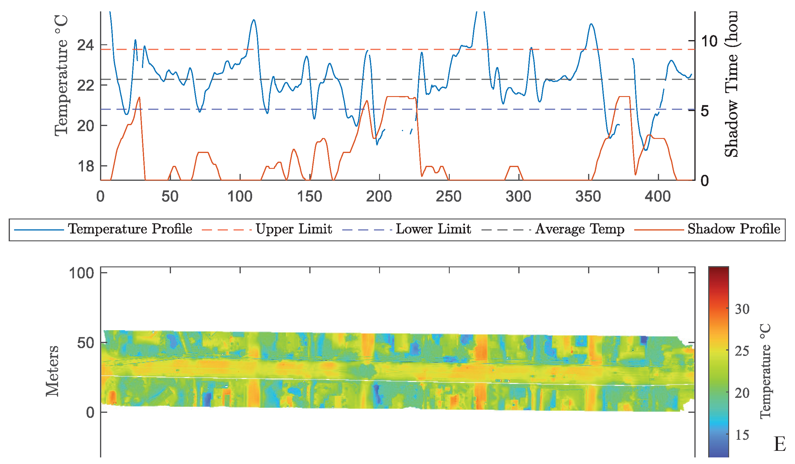
Based on the results of the field tests, the team found it necessary to develop a model to predict the location and time of shadows based on the surrounding landscape. During the analysis of the field test results, it was observed that the temperature effects of shading before sunset are still present in the subsequent morning and the correlation between the two is apparent. These shadow effects were significant and were initially a source of false alarms. The temperature map of Rural Rd at 4:41 a.m. on 31 May 2023 best illustrates this phenomenon (
Figure 1). In this image, the cooler thermal signature left by shadows of the trees before sunset can be seen cast onto the road the following morning.
To produce the shadow model, the DEMs were utilized to provide the height values of the structures present at the sites. Using a MATLAB script, the mode of the elevation was defined as ground level. Then, the ground level was subtracted from the elevation of each pixel providing the height of each of the objects. With this, the length of the shadows could be calculated as S = h/tan(A) [
19], where h is the height of the object, S is the shadow length, and A is the solar elevation. The solar elevation was calculated using the open source MATLAB script [
20]. This script produces the solar elevation and the azimuth based on the latitude and longitude and time of day. Any pixel wherein the height was below 2 m was neglected. For each pixel, the lengths of the shadows were calculated in meters and then converted to pixels based on the pixel size of each temperature map. Then, using Bresenham’s line algorithm optimized for MATLAB, lines were drawn from the original pixel to the corresponding end pixel based on the azimuth and shadow length [
21]. This process was repeated for each pixel with a height value.
The azimuth and shadow elevation were calculated for the twenty-four-hour period before the flight time to obtain the shadow time. Based on the result of an initial twenty-four-hour analysis, the period was reduced to 6–9.5 h by quantitatively comparing the correlation of shadow time to the temperature profile for each time interval between 1 and 12 h. The optimal time intervals were determined to be 6–9.5 h as it provided more weight to the shading close to the flight time and neglected the position of shadows further from the time of the flight. The team found that 6 h of shading provided the best correlation for roads oriented north to south and 9.5 h for roads oriented from east to west. The results of this quantitative correlation analysis can be found in
Appendix A.
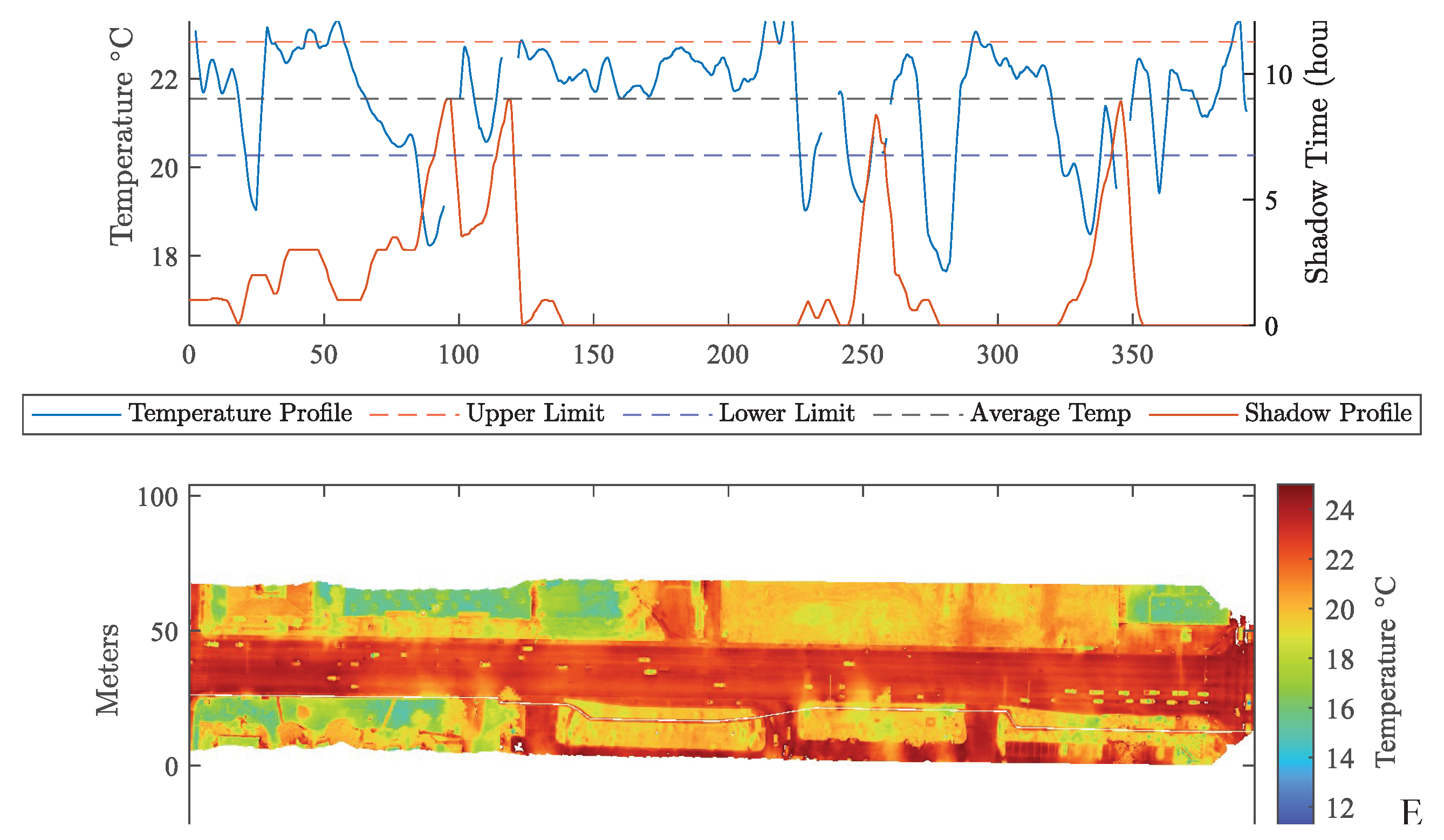
The shadow time profile was plotted along the same path of pixels as the temperature profile. In addition, the contour lines of the shadow time matrix were plotted on top of the grayscale thermal image beneath the thermal profile. To determine the accuracy of the shadow profile, an initial shadow map was plotted on the data collected at 9:04 a.m. along 24th St. This dataset was chosen as the sun had risen at this time casting shadows onto the street (
Figure 2). These shadows can clearly be seen in the thermal image and provide an excellent reference for the shadow model. This figure shows the contours of the shadow model plotted on top of the temperature map for 24th St at 9:04 a.m. on 30 November 2023, and highlights the close agreement between the model and the shadows. Shadows from tall thin objects were neglected in a filtering stage to reduce noise. This simplification had a minimal effect on the results as shadows from tall thin structures move fast enough and are small enough to not significantly influence surface temperatures.
This shadow model served as a proxy for the solar energy input into the system, where places with larger shadow times received less solar energy than areas without the presence of shadows. By using the shadow model and the Bird Clear Sky model, an estimated power flux was derived and integrated in time to calculate energy in ten-minute intervals. Then, the profile of the energy was calculated along the same path as the temperature profile for each dataset. This energy model directly described the energy input correlated to the temperature map and provided verification for the shadow model.
When the temperature profiles were plotted against the energy profile, the temperatures closely correlated to the energy profile (see
Figure 3). However, one pattern of discrepancy between these two correlations was caused by the presence of the trees. For the flights flown in the late fall and winter months, the temperature of the ground near the location of trees remains warmer throughout the night. For the shadow model, the area around the trees was covered by shadows throughout the day. The hypothesis of the causes of these warm ground temperatures was the fact that the trees prevented heat loss from the system caused by nocturnal radiative cooling as the trees reduced the view factor of the surface to the sky. This phenomenon is expected to reverse during hot summer nights causing the ground temperature near trees to be cooler than the surrounding temperature due to the increase in solar irradiance during the day, negating the impact of preventing nocturnal radiative cooling.
The shadow model was then applied to the temperature profiles of each of the seven known leak sites that were evaluated. The result of the data fusion process between the shadow time and temperature profile is described below. One dataset that clearly illustrates the correlation between surface temperature and shadow time is the 24th St flight taken before sunrise at 6:15 a.m. on 30 November 2023, shown in
Figure 3. Although these images were acquired at 6:15 a.m., there was a significant correlation of surface temperatures to the shadow profiles before sunset the day before. The 6 h of sunlight before the flight were 11:15 a.m. to 5:15 p.m.
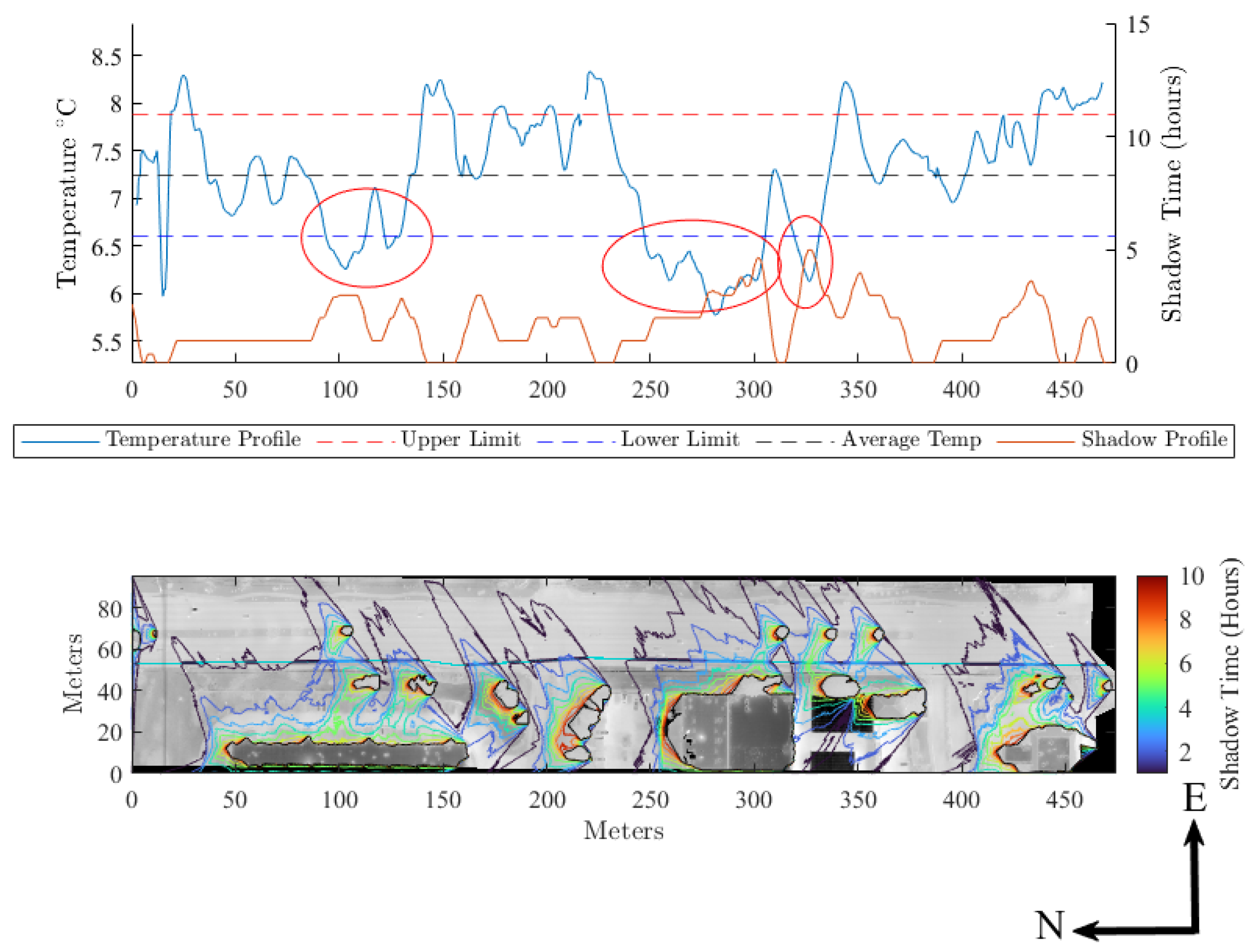
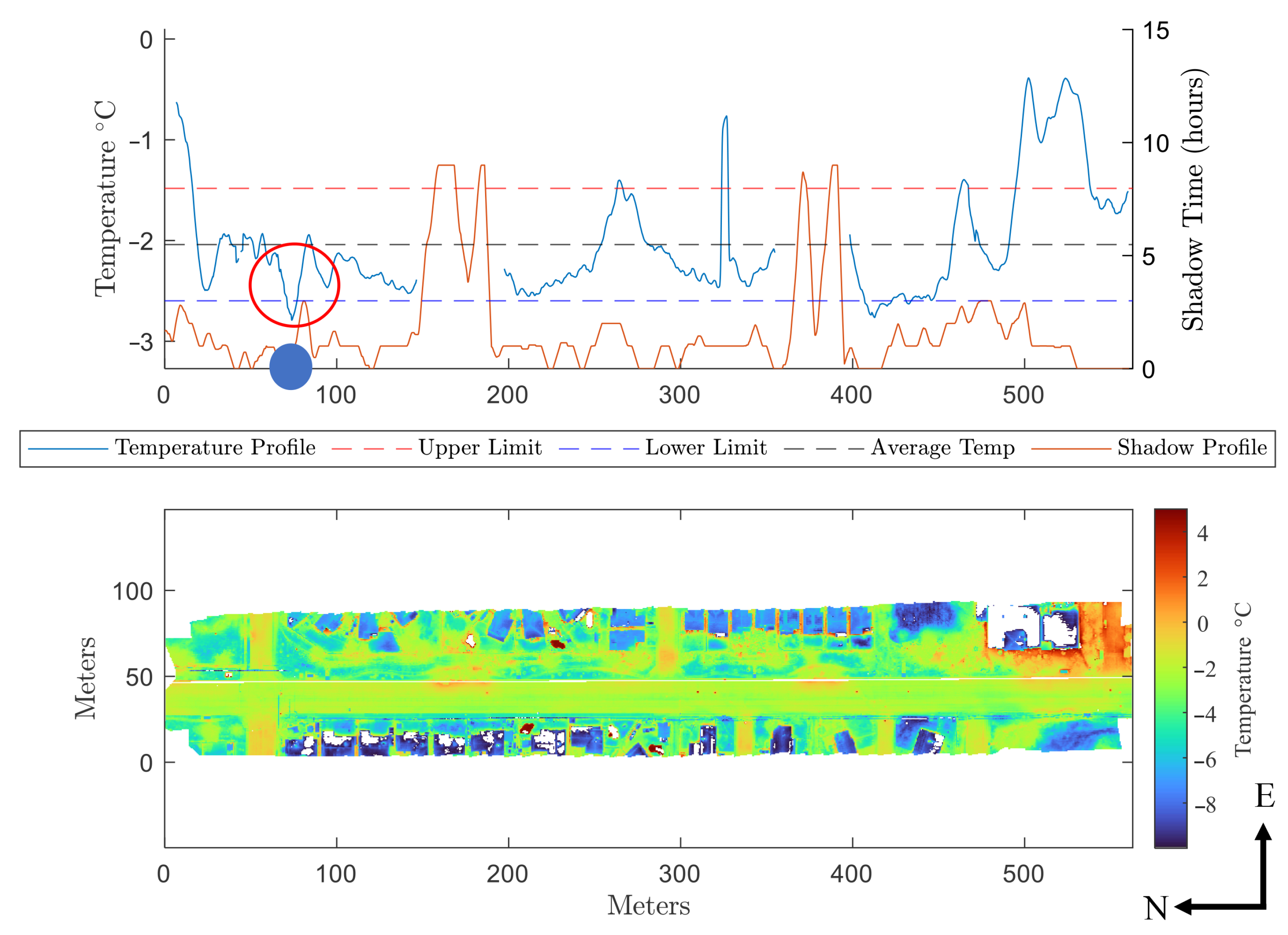
Using these shadow time graphs with the contour plots, the initial POIs for each flight defined before shadows were considered were re-evaluated with an additional criterion of whether there was a significant increase in shadow time at the same location as a potential POI. With this criterion, several of the POIs initially defined in the field test results were excluded. One dataset that illustrated the usefulness of filtering POIs with a shadow model is the 5:37 McQueen Road dataset found in
Figure 4. At the location of the original first POI, highlighted with a red circle, there is a high shadow time. This indicates that the first POI is likely not caused by the known leak in this area, but instead by the presence of shadows. The other two POIs were likely caused by shadows as well.
3.5. Field Test Data Processing
The first step in the processing program was importing the orthomosaics and extracting the temperature data, GPS coordinates, and elevation data. These values were then organized into separate matrices and were transposed based on the orientation of the site to ensure that each would have the same orientation during the graphing stage. Initially, a grayscale temperature map was plotted. This initial plot was used to manually select pixel coordinates that would determine the path of the temperature profile. This path was selected to follow the path of the CIPP with a potential leak, and the locations of these CIPPS were provided by SRP. Once several coordinates were chosen, between 3 and 10 depending on the complexity of the path, a straight line of pixels between each set of coordinates was created using linear interpolation. This line was then expanded from a width of one pixel to a width of seven pixels perpendicular to the original interpolated line path. Seven pixels is equivalent to between 0.6 and 1.5 m in width depending on the altitude the original images were taken. This width was chosen to fit within the width of an average sidewalk in the Phoenix area, underneath which water pipelines are often buried. The average temperatures were calculated for each set of seven pixels along this path. For the test flights, a moving average with an averaging window of 3–5 m was used to smooth this data. A window size of 3–5 m was chosen based on the results of numerical simulations of potential pipe leaks conducted using the software Hydrus 2D (Version 2.103) [
15]. The numerical simulations suggested leaks would increase the soil moisture levels in a region approximately 3–5 m in length beneath a sidewalk surface layer.
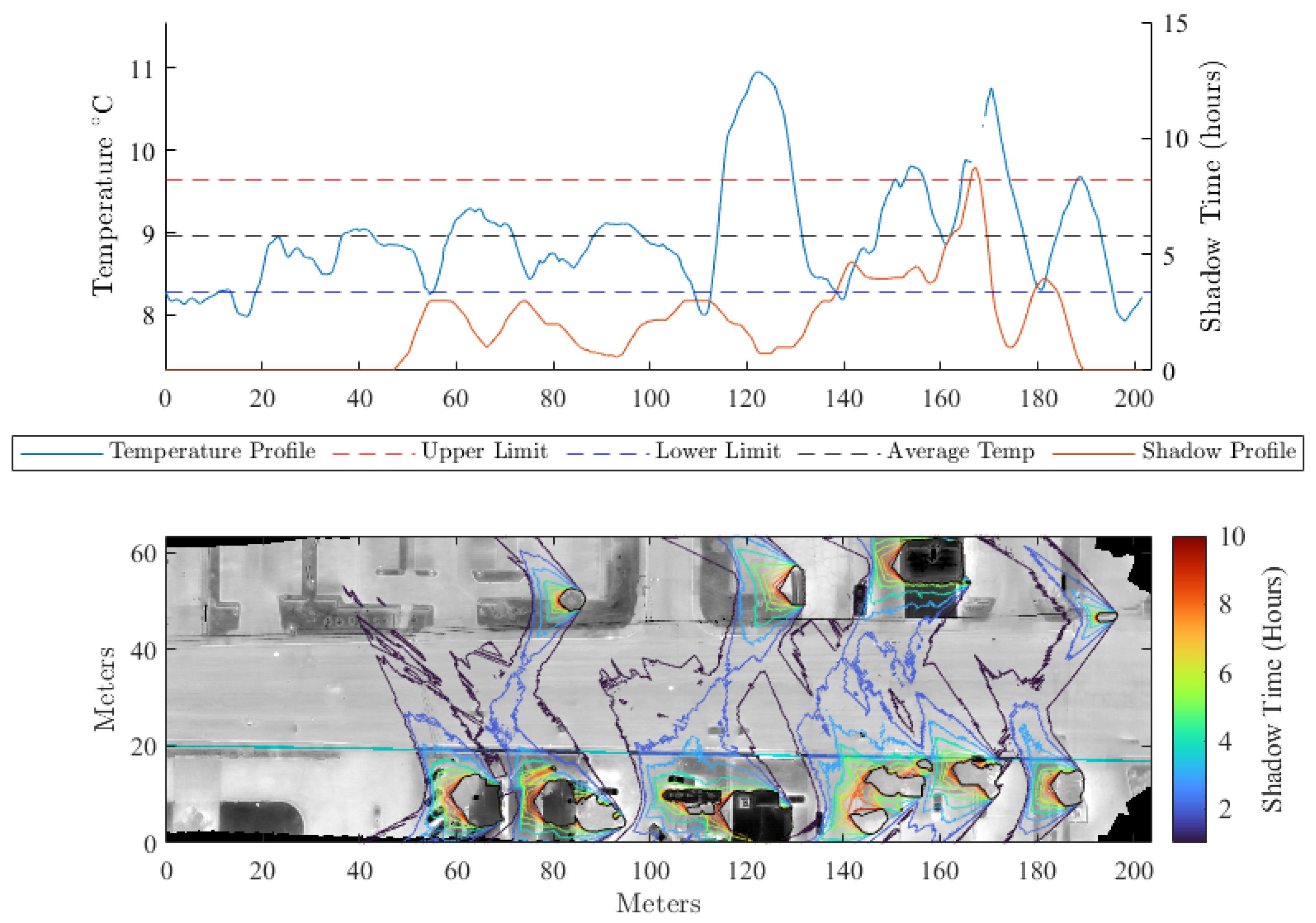
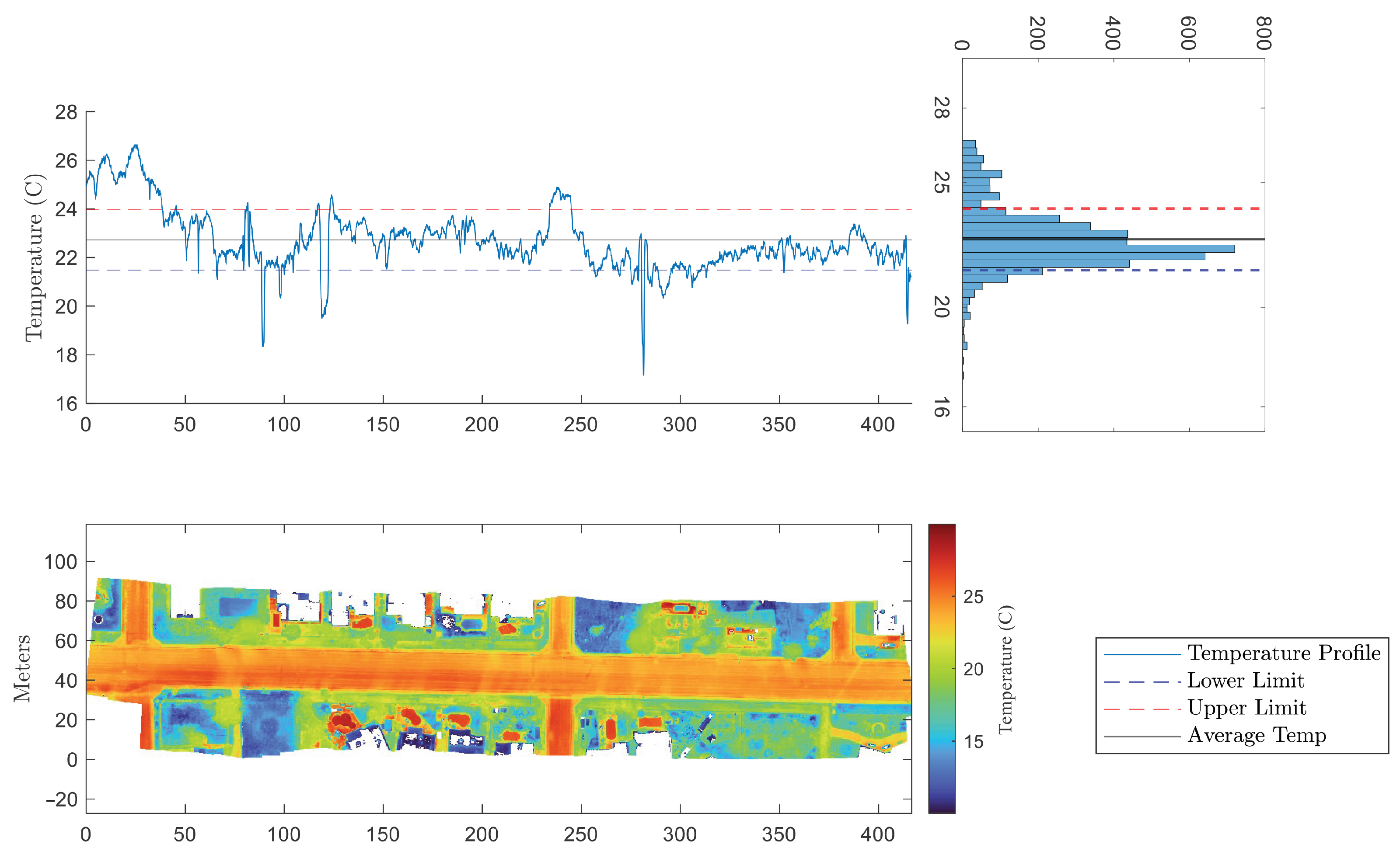
The temperature profile was then plotted along with the average temperature along the path, and the upper and lower detection limits were defined as ±1 standard deviation in temperature along the route. An upper and lower boundary was set to 1−
from the mean temperature. The temperatures in the profiles are approximately normal, as shown in
Figure 5; however, a higher percentage of data falls within 1−
from the mean than a true normal distribution. It was observed that between 70 and 78% of the temperature was within 1 standard deviation from the mean. We therefore used 1−
as the initial threshold for developing points of interest.
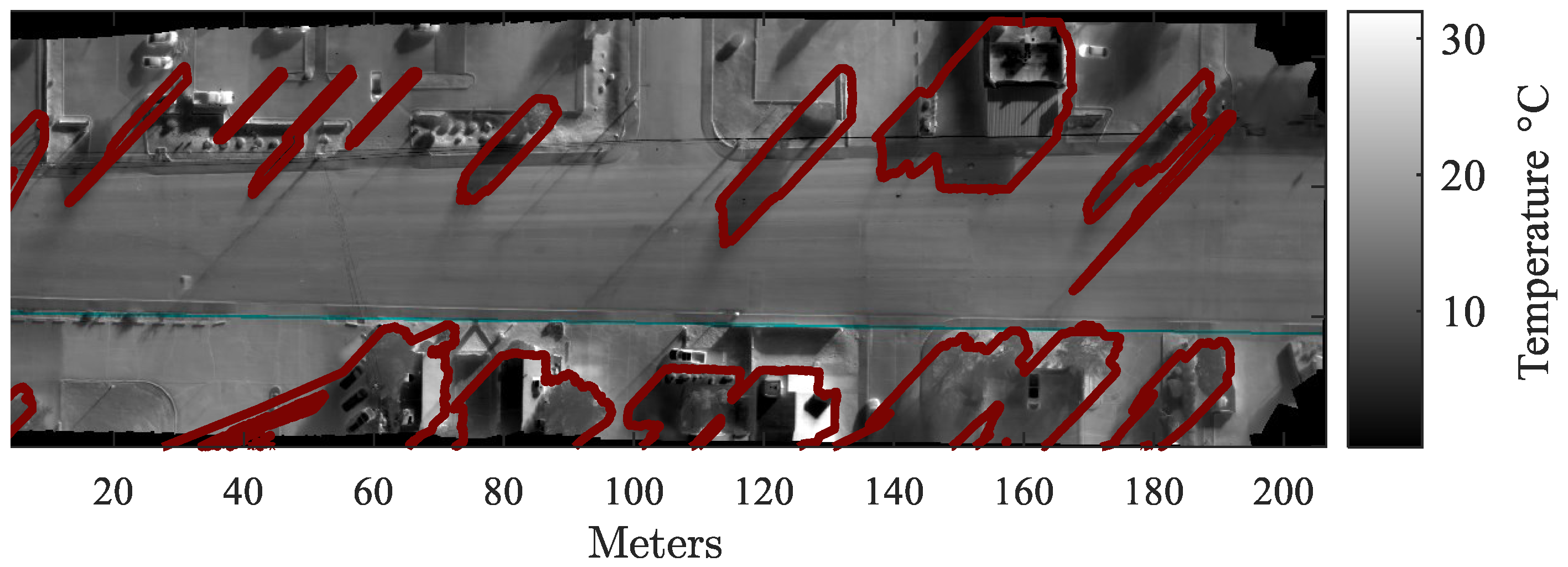
A linked temperature profile on a color image plot served as a final check of potential points of interest to determine whether an external factor such as metal manhole/access covers, vegetation, and other objects not properly captured by the elevation map caused cold spots in several datasets.
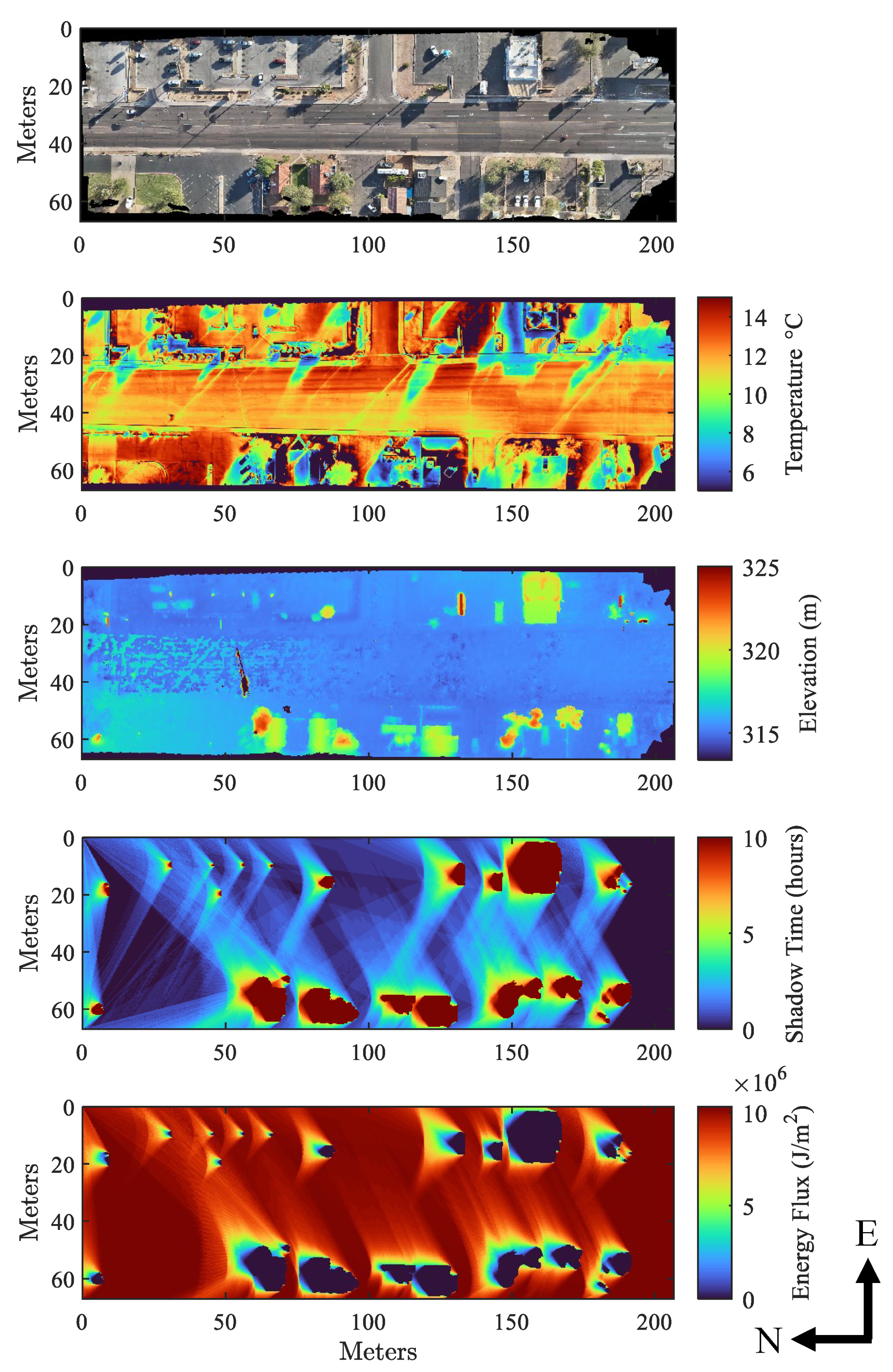
Figure 7 illustrates the integrated visible orthomosaic, the grayscale IR image, the digital elevation model, the shadow model, and the energy model products used for leak detection.
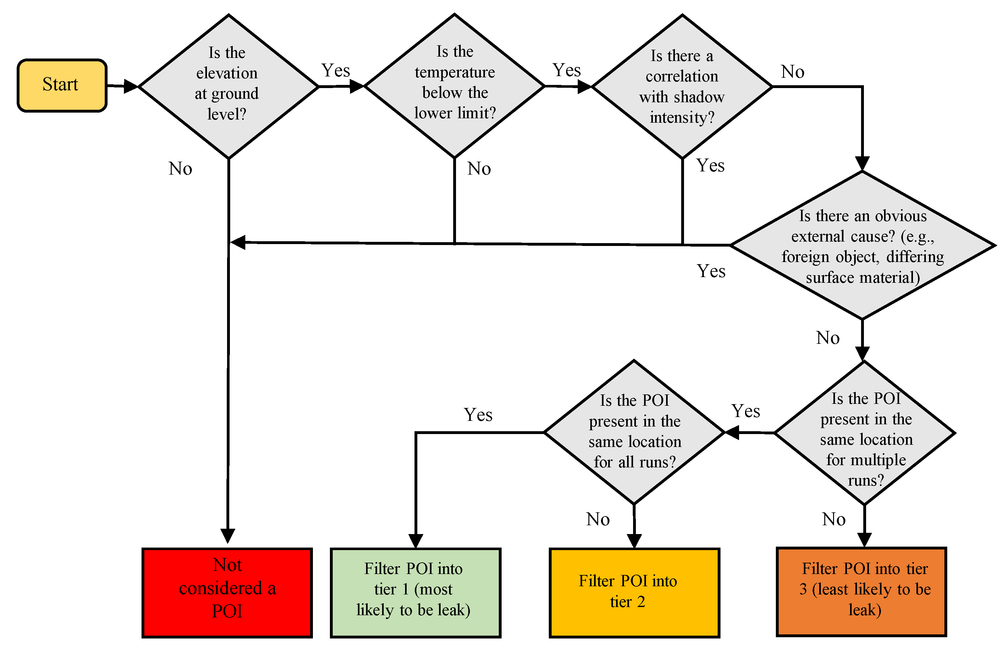
To determine which cold spots would be defined as the final points of interest the temperature profiles, temperature maps, and shadow time profiles were analyzed. Additionally, all POIs were organized into a tiered list. Points of interest that were present in the same location for all of the flight data for each known leak site were categorized as tier 1, having the highest potential to be a signal of a known leak. POIs that were present in multiple sets of flight data were defined as tier 2, and POIs only present in one dataset were classified as tier 3. A logic diagram of the filtering process used to define which cold spots were representative of POIs and the tier of each POI is located in
Figure 6.
Figure 6.
Example of the data products used to evaluate the leak sites and define POIs including, in order from top to bottom, color image orthomosaic, IR orthomosaic, digital elevation map, shadow model, energy model based on the data collected at 24th St at 6:15 a.m. on 3 November 2023.
Figure 6.
Example of the data products used to evaluate the leak sites and define POIs including, in order from top to bottom, color image orthomosaic, IR orthomosaic, digital elevation map, shadow model, energy model based on the data collected at 24th St at 6:15 a.m. on 3 November 2023.
Figure 7.
Flow diagram of the process used to filter points of interest.
Figure 7.
Flow diagram of the process used to filter points of interest.
4. Results
For the field test, seven sites were evaluated; five sites with known leaks, and two sites that served as controls. For the sites with a known leak, an identifiable thermal signal was detected around the location of the known leak for four out of the five sites. Along with these known leaks, several points of interest were defined using the logical methods described in
Section 3. Multiple flights were flown for each known leak site between sunset and sunrise.
4.1. Camelback Road
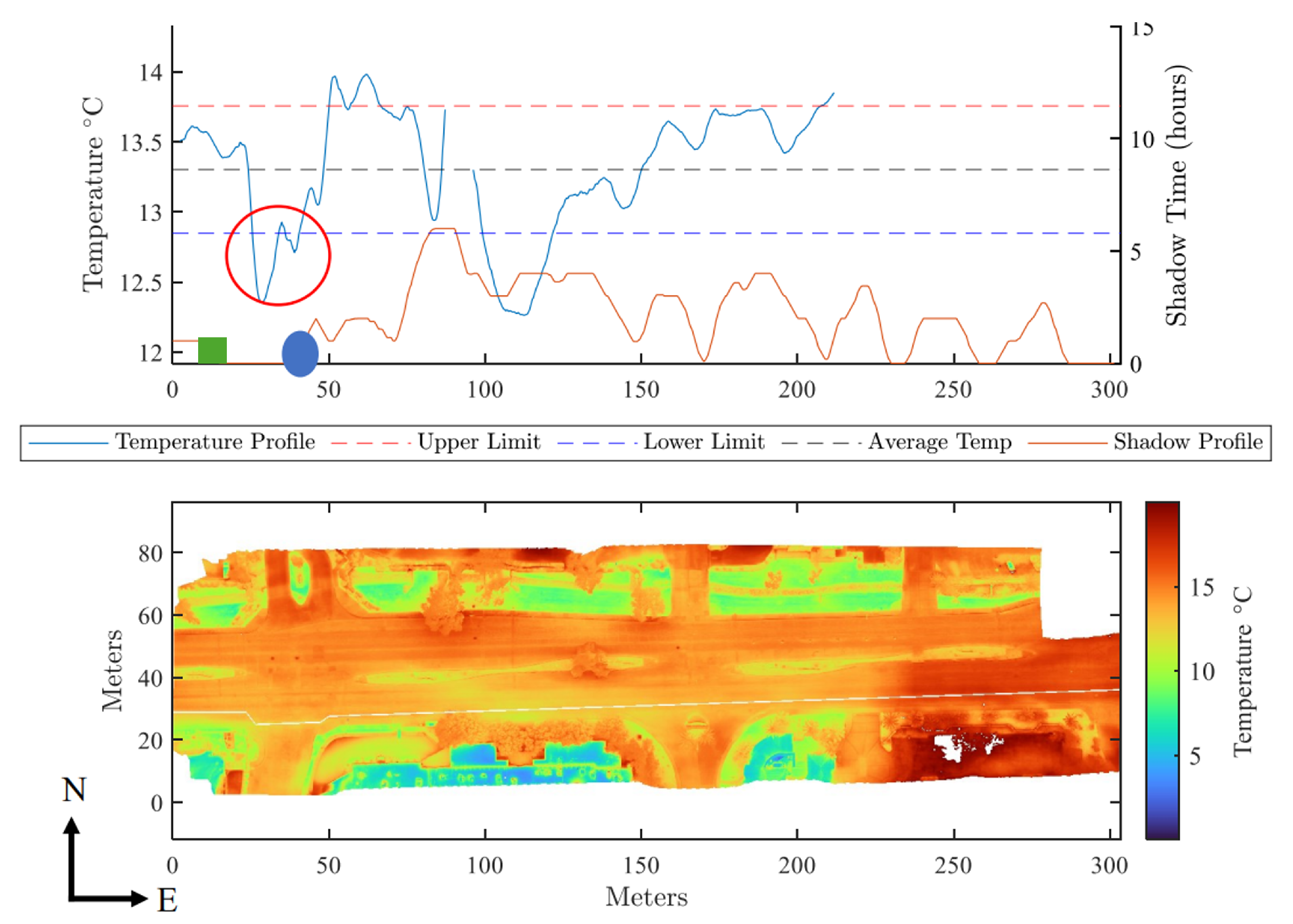
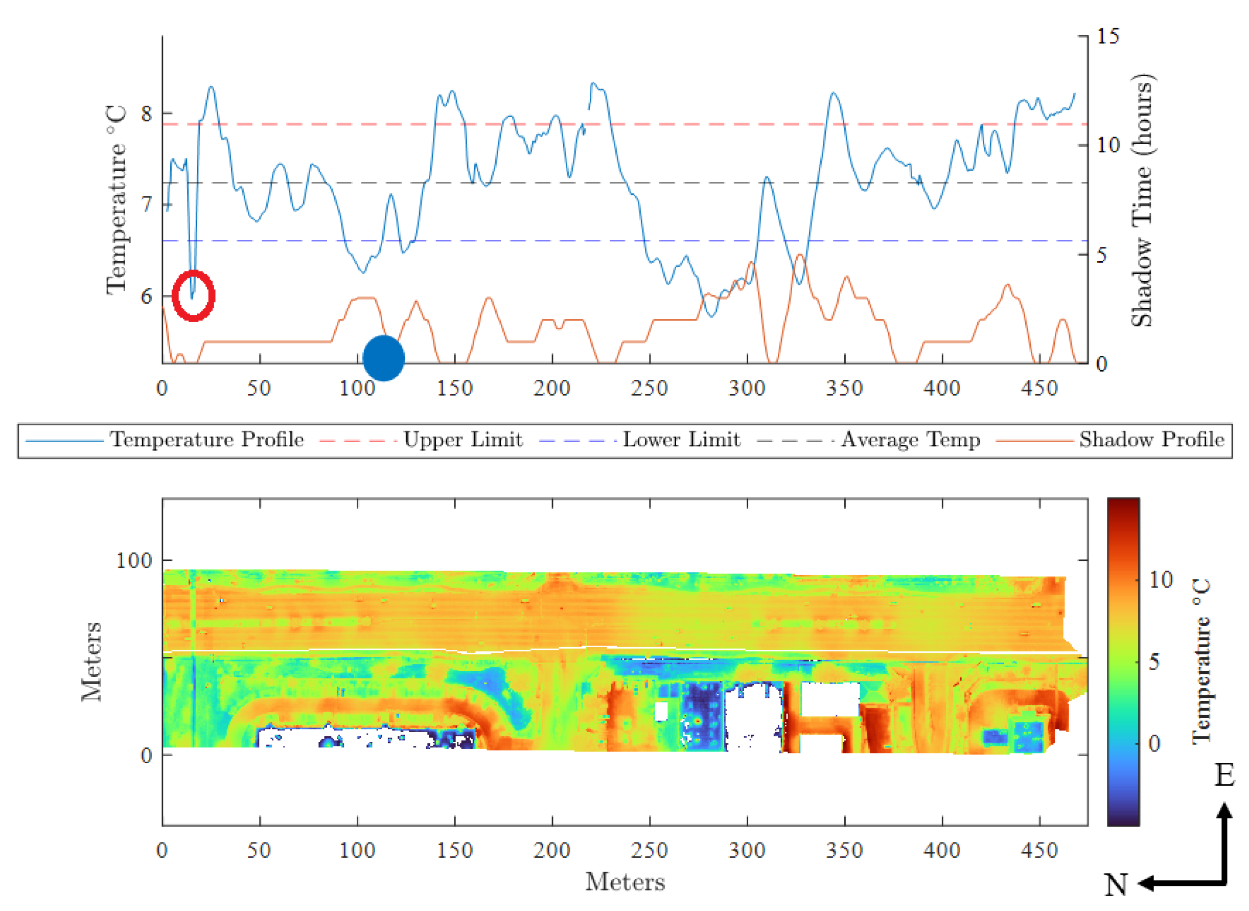
For the potential leak that was located along the side of Camelback Road, two flights were flown, once at 10:03 p.m. on 29 November 2023, and again at 5:50 a.m. the following day. This site was unique because a large portion of the east side of the road was much warmer than the west side. The cause of this increased temperature is unknown. To ensure that this abnormally warm section would not inflate the mean and the standard deviation of the entire temperature profile, this section was neglected.
Figure 8 contains the temperature profile and temperature map for the first Camelback Rd test at 10:32 p.m. with the location of the points of interest denoted by red circles and the location of the leak with a blue circle.
The location of the known leak, as defined by SRP, is located at approximately 45 m. The location of the first point of interest overlaps with the location of the known leak at this leak site. The first point of interest begins 22.5 m from the left water gate and is approximately 25 m in length. A second and third point of interest were defined and both are located further east, 99 m and 140.5 m from the start position, respectively. Both the second and third POIs were not present in both flights and were thus defined as tier 3 POIs.
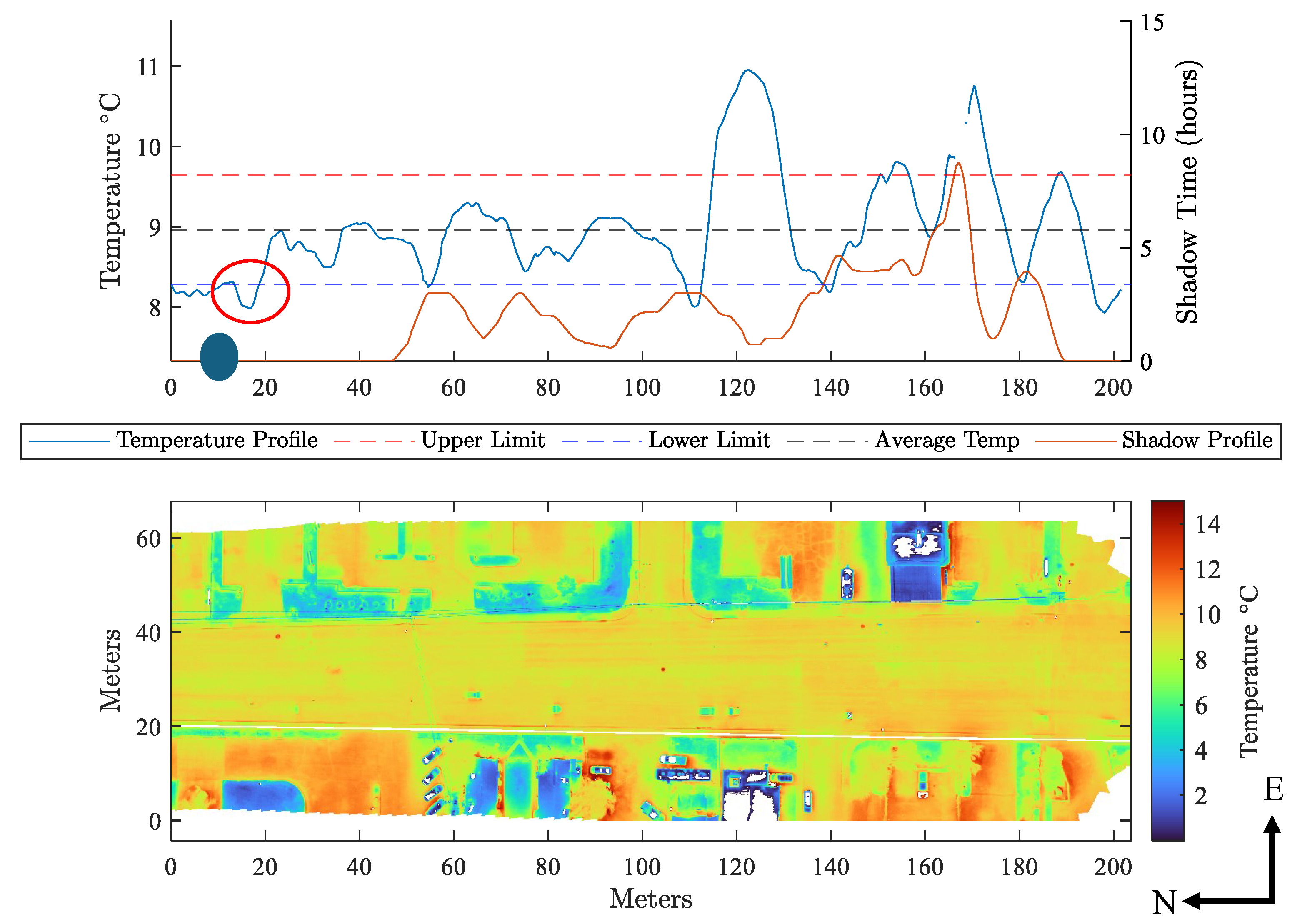
4.2. 24th Street
The next location that the team assessed lies along 24th Street in Phoenix. For this site, three datasets were collected at 5:46 p.m. on 29 November 2023, and twice more the following morning at 6:15 a.m. and 9:04 a.m. During the 6:32 a.m. test flight, what seemed to be an apparent cold spot was found along the road. Thus, the team returned later in the morning to re-fly this area. The temperature profile of the 6:15 a.m. flight is shown in
Figure 9.
SRP identified a known leak at approximately 9 m. The first POI was 10 m from the maintenance hole cover and was around 9 m in length. This POI is the closest to the leak and was determined to be partially overlapping the known leak due to its proximity. According to SRP, the water from the leak can present itself up to 33 m from the actual leak site, which means the first POI has the potential of being caused by the known leak. The first POI was defined as a tier 2 POI as it was present in multiple flights. Three other POI were defined for this leak site and the positions of each relative to the start position can be found in
Table 1. The cold spot located at 198 m was caused by powerlines.
4.3. Elliot Road
The next known leak site was located along Elliot Road in Gilbert. Four datasets were collected at this site. The first dataset was collected at 8:36 p.m. on 29 November 2023. This was the only dataset taken of this road on this day that was able to be processed into an orthomosaic due to an error in the data collected. Additionally, flights were flown later on the 5th or 6th of January 2024 at 6:04 p.m., 9:40 p.m., and 6:32 a.m.
Figure 10 shows the results from the flight conducted at 8:36 p.m.
According to SRP, the known leak was 15 m East of Neely Road, which runs north to south at the leftmost edge of the temperature map. There was only one POI that the team established for this dataset that overlapped with this leak. This point of interest begins at 73 m and is 28 m in length. The POI overlaps the location of the known leak. In addition, this point of interest is present in both data collected in November and January and was defined as a tier 2 POI. The presence of this leak on different nights a month apart strengthens the argument that it is caused by a leak. Two other POIs were defined for this leak site and the positions of each relative to the start position can be found in
Table 1. The cold spot located at 431–434 m was caused by a storm drain.
4.4. McQueen Road
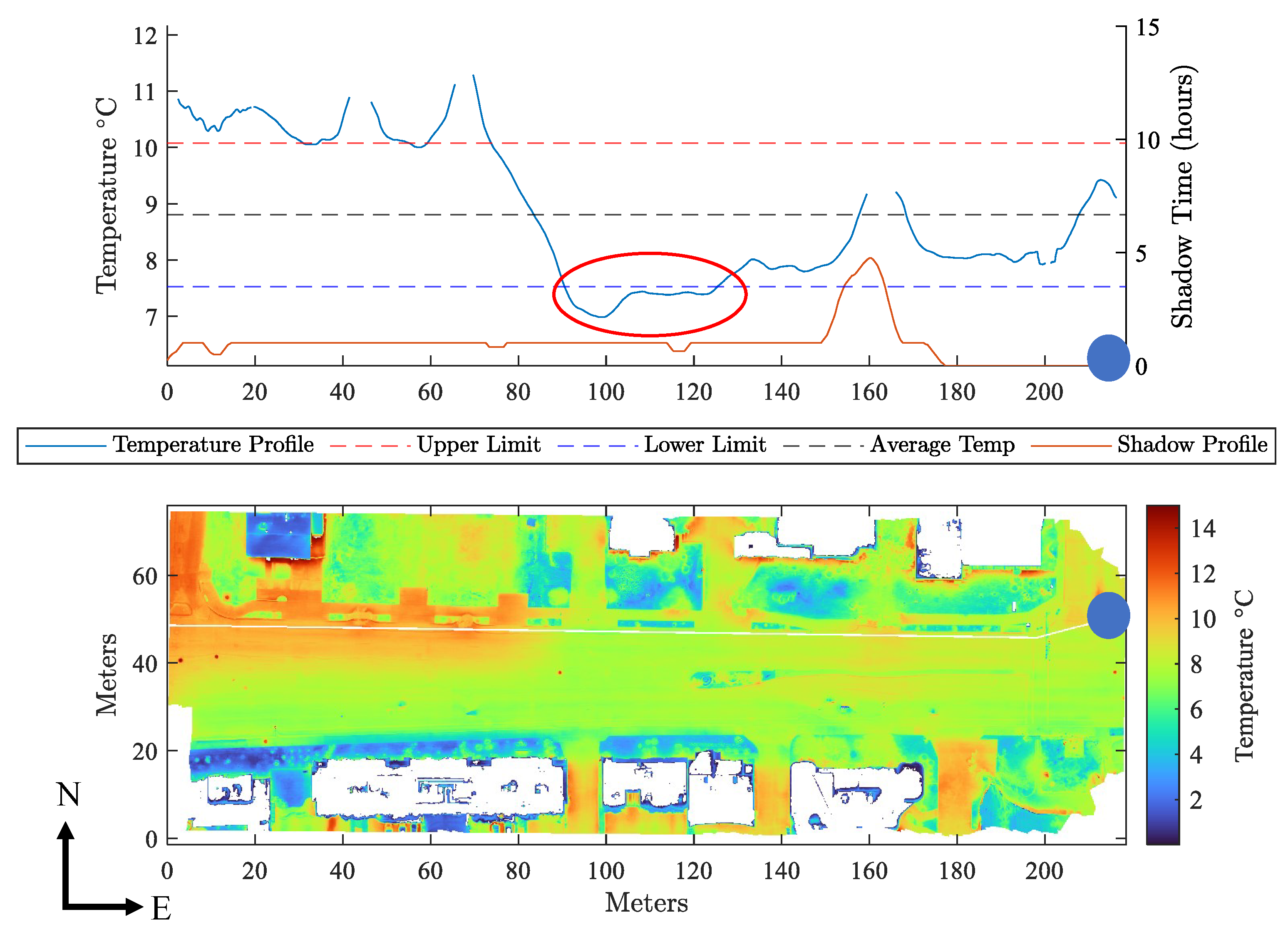
The next known leak site that was evaluated was located along McQueen Road in Gilbert. This road was assessed on the 5 and 6 January 2024. The team collected three different datasets for this site, one at 5:37 p.m., another at 10:03 p.m., and the last the morning of the 6th at 6:12 a.m.
Figure 11 contains the resulting temperature map and temperature profile for 5:37 p.m. with the location of the points of interest, the location of the water gate, and the location of the leak.
The known leak was located 137 m from a water gate just to the left of the temperature map. The watergate was not captured in the temperature map as it is located below power lines the team was unable to safely fly over. None of the three POIs determined at this leak site overlap with the known leak. There is a significant thermal signal present from 85 to 140 m around the known leak but this thermal signal was likely caused by the lingering temporal effect of shading as determined by the high correlation between temperature and shadow time, as seen in
Figure 11. The location and tiered ranking of the three POIS can be found in
Table 1. The cold spot located at 14–17 m was caused by power lines.
4.5. Thomas Road
The last known leak site was located on Thomas Road between N 73rd St and N 74th St in Scottsdale, AZ. Two flights were taken of this site. The first at 6:18 p.m. on 29 November 2023, and the second on the following morning at 6:44 a.m. on the 30th.
Figure 12 contains the resulting temperature map and temperature profile for the 6:44 a.m.
The known leak is located 9 m west of a water gate just to the right of the temperature map. For this run, no POIs were found overlapping the location of the known leak. Although there were four POIs total, the location of these POIs was not constant from one run to another; thus, both POIs were defined as tier 3 POIs. The location of both POIs can be found in
Table 1.
4.6. North 15th Avenue and 7th Street (Control Sites)
During the field testing, two control sites were evaluated. Both locations previously had known leaks but the pipes had been inspected and repaired before testing. As such, these sections had a low probability of containing active leaks. Both sites were only flown once due to time constraints for field testing. The first site, 15th Ave, was flown once at 3:57 p.m. on 29 November 2023. This temperature profile for this site is shown in
Appendix B with a table containing the causes of the cold spots not defined as a POI. The jumps in the data indicate where the elevation was 1 m above ground level and these temperatures were disregarded as they were caused by trees over the path of the temperature profile. In reviewing this data, no points of interest were found. Each cold spot was caused by external factors such as foreign objects or shading. Shading was the main cause of the cold spots present such as for the cold spot at 150 m. The temperature data for 7th St was collected at 4:45 p.m. on 29 November 2023. The temperature profile for 7th St is shown in
Appendix B. Once again, each cold region was caused by external factors similar to those along 15th Ave.
4.7. Summary of Results
There were several more tier 3 POIs than tier 1 and tier 2 POIs with a total of 14 POIs that were defined as tier 3, 3 POIs that were defined as tier 2, and only 1 POI that was defined as tier 1. The shadow model showed a high correlation between the POI that was thought to overlap with the known leak at the McQueen Road site; thus, it was removed as a POI as it no longer fit the definition. When shadows were considered, the detection rate decreased to 50% from the original 62.5%. In addition, the rate of false negatives then increased to 37.5%.
Table 2 summarizes, for each known leak site, the updated amount of POIs when shadows were considered, the number of POIs in each tier, and the known leak sites that had a POI that overlapped with the position of a known leak specified by SRP. An automated POI classification has not yet been used since the terrain and composition of the roads result in many temperature drops that are not representative of any possible leak (manhole covers, water access covers, etc.).
These results show promising capabilities for this system. These false negative and true positive rates can be reduced and increased, respectively, by the collection of more data on a variety of dates to help filter out elements that can pose a temperature drop. This also works with the POI classification system, as if there is more data and a POI appears on all, that is a clear sign that there is a high-confidence POI there that could indicate a leak.
5. Discussion
It has been observed that drone-based infrared imagery can be utilized to remotely and noninvasively sense thermal signatures of abnormal soil moisture underneath urban surface treatments caused by the leakage of water pipelines during the regular operation of water transportation. For the eight sites tested with known leaks during both sets of field tests, a thermal signal was detected around the known leak for five sites or an overall rate of detection of 60%. Although it is not possible to make a definite conclusion about the rate of false positives and false negatives at this stage because of the small sample size, these values were calculated to provide a benchmark for use in the future phases of this project.
This research leaves large open questions that will need additional research efforts to answer properly. The rate of false negatives based solely on when no thermal signal was detected at the location of the known leaks was 40%. The rate of false positives was not calculated as no POIs were detected at the two control sites (N 15th Ave and 7th St). This is a promising result but does not allow the team to make any definite conclusions about the rate of false positives. During both sets of field tests, the team observed cold spots in the temperature profile and temperature maps that seemed to be caused by shadows. Shadows are a factor that complicates the detection method as they can appear as false negatives.
This methodology requires flights to be performed several times, often on different days and times of day. This means that there will inherently be different thermal profiles than on other days. While this difference is noticeable, the trends are what is important for the success of the project. As long as the line of analysis is consistently made along/adjacent to the pipe location, the trends of the thermal signature should be consistent. Having these flights conducted on different days can increase the POI detection confidence since, if there is a POI that presents itself on each flight, this is an even stronger indication that the POI could be a leak. Consistency is key with this methodology, so maintaining the same drone/camera is critical throughout the POI analysis.
Additional testing would provide a better understanding of the accuracy by allowing the team to calculate the true rate of false negatives and false positives. It was not realistic to calculate the rates of type 1 and type 2 errors at this stage in the project because the team could only base the false positive and negative rates on the known leaks provided by SRP which was a limited sample size. The team was unable to determine the rate of false positives from the POIs because verifying whether each POI was a false positive required inspecting the interior of the pipe or excavating the POI locations, neither of which were feasible. Additionally, the rate of false negatives was solely based on the known leaks provided to the team by SRP but this sample set did not represent the true rate of false negatives. The true rate of false negatives could not be evaluated as SRP does not have a method for effectively determining the location of every leak in a CIPP system. Without knowing the location of all leaks in a system, it was not possible to assess the temperature data to determine whether the locations would have been a POI. The team intended to map several more sites before SRP conducted annual maintenance and inspections on the CIPPS during the winter months.
6. Conclusions
Over the course of this study, it was observed that shading before sunset continued to affect surface temperature into the hours before sunrise. To account for this phenomenon, a shadow model was generated to estimate the position of shadow at any time during the day based on the structures surrounding each known leak site. This shadow model was used to filter the POIs to neglect cold spots caused by shadow. This model removed several of the original POIs; most notably, the first POI from the McQueen Road dataset which overlapped with the known leak. The correlation between the shadow time and temperature was present in all datasets, even those taken early in the morning before sunrise. This observation indicates that the position of shadows needs to be quantified to account for these lasting temporal signatures in infrared detection endeavors. Additionally, considering an elevation dataset while filtering areas of interest allowed for a reduction in false positives caused by interfering structures found in an urban setting. The implementation of the datasets enhanced the detection accuracy while also significantly reducing the time and labor involved compared to traditional methods. The detection rate of the known leak was determined to be 60. These findings also suggest that infrared thermography, particularly when augmented by advanced data processing techniques, represents a valuable tool for municipal water management systems, offering a proactive approach to identifying and addressing infrastructure leaks. Currently, the developed filtration method completely neglects cold spots where shading is present. In the future, this filtering shadow model can be used to account for the shadow location and the corresponding temperature change to determine POI in locations with heavy shadow locations.
Due to the few pin-pointed leaks that were provided, the determination of Types 1 and 2 errors are difficult to quantify and thus may not fully represent the efficacy of the methodology. The team is exploring other methods of analysis to confirm a POI as a leak, but has yet to be implemented into the project. This method entails determining soil moisture as soil depth increases. By comparing the soil moisture profile of the potential leak location at the high-confidence POI to a control site adjacent to the POI, the team can compare the results and determine whether that POI was likely to be a leak.
Author Contributions
Conceptualization, M.S., Z.D., Y.X., A.W.J. and L.C.; methodology, M.S., Z.D. and L.C.; software, L.C.; validation, M.S., Z.D. and L.C.; formal analysis, L.C.; investigation, L.C.; resources, L.C.; data curation, L.C.; writing—original draft preparation, L.C.; writing—review and editing, M.S., Z.D. and R.D.; visualization, L.C.; supervision, M.S., Z.D., Y.X. and A.W.J.; project administration, M.S. and Z.D.; funding acquisition, M.S. and Z.D. All authors have read and agreed to the published version of the manuscript.
Funding
This research was funded by the University Research Project sponsored by Salt River Project.
Data Availability Statement
The original contributions presented in this study are included in the article. Further inquiries can be directed to the corresponding author.
Acknowledgments
The authors would like to acknowledge the Salt River Project for their continued funding and support behind the project.
Conflicts of Interest
The authors declare no conflicts of interest.
Abbreviations
The following abbreviations are used in this manuscript:
| SRP | The Salt River Project |
| CIPP | Cast-In-Place-Pipes |
| IR | Infrared |
| CCTV | Closed Circuit Television |
| UAV | Unmanned Aerial Vehicle |
| TIR | Thermal Infrared |
| USGS | United States Geographical Survey |
| POI | Point of Interest |
Appendix A
Table A1.
Normalized cross-correlation values for the number of sunlight hours considered in the shadow model and the temperature profile for each potential leak site (max cross-correlation factor highlighted in green).
Table A1.
Normalized cross-correlation values for the number of sunlight hours considered in the shadow model and the temperature profile for each potential leak site (max cross-correlation factor highlighted in green).
| Hours of Sunlight | McQueen Rd | 24th St | Elliot Rd | Camelback Rd | Thomas Rd |
|---|
| 0.5 | 0.9773 | 0.8797 | 0.7758 | 0.7206 | 0.8786 |
| 1 | 0.9790 | 0.9513 | 0.7743 | 0.8044 | 0.8721 |
| 1.5 | 0.9777 | 0.9635 | 0.8018 | 0.8764 | 0.8847 |
| 2 | 0.9787 | 0.9635 | 0.8521 | 0.9181 | 0.9142 |
| 2.5 | 0.9838 | 0.9635 | 0.8982 | 0.9503 | 0.9327 |
| 3 | 0.9868 | 0.9635 | 0.9257 | 0.9670 | 0.9430 |
| 3.5 | 0.9882 | 0.9635 | 0.9419 | 0.9757 | 0.9507 |
| 4 | 0.9888 | 0.9635 | 0.9529 | 0.9808 | 0.9556 |
| 4.5 | 0.9888 | 0.9635 | 0.9605 | 0.9838 | 0.9585 |
| 5 | 0.9888 | 0.9635 | 0.9659 | 0.9856 | 0.9622 |
| 5.5 | 0.9888 | 0.9552 | 0.9697 | 0.9864 | 0.9632 |
| 6 | 0.9888 | 0.9691 | 0.9728 | 0.9866 | 0.9632 |
| 6.5 | 0.9888 | 0.9686 | 0.9754 | 0.9858 | 0.9632 |
| 7 | 0.9871 | 0.9650 | 0.9776 | 0.9841 | 0.9632 |
| 7.5 | 0.9796 | 0.9608 | 0.9794 | 0.9818 | 0.9632 |
| 8 | 0.9730 | 0.9564 | 0.9809 | 0.9793 | 0.9628 |
| 8.5 | 0.9667 | 0.9517 | 0.9821 | 0.9772 | 0.9644 |
| 9 | 0.9601 | 0.9467 | 0.9829 | 0.9747 | 0.9670 |
| 9.5 | 0.9551 | 0.9419 | 0.9834 | 0.9717 | 0.9671 |
| 10 | 0.9525 | 0.9419 | 0.9834 | 0.9685 | 0.9667 |
Appendix B
Figure A1.
North 15th Ave temperature profile and TIR temperature map. The gaps in the data at 200–230 m and 360–370 m were caused by trees over the sidewalk and were removed by the Matlab algorithm.
Figure A1.
North 15th Ave temperature profile and TIR temperature map. The gaps in the data at 200–230 m and 360–370 m were caused by trees over the sidewalk and were removed by the Matlab algorithm.
Figure A2.
7th St temperature profile and TIR temperature map.
Figure A2.
7th St temperature profile and TIR temperature map.
Table A2.
List of cold spot locations and the cause or the reason it was not defined as POI for N 15th Ave and 7th St.
Table A2.
List of cold spot locations and the cause or the reason it was not defined as POI for N 15th Ave and 7th St.
| N 15th Ave | 7th St |
|---|
| Location (m) | Cause | Location (m) | Cause |
| 16–20 | Shadow | 21–36 | Access Cover |
| 70–72 | Power lines | 85–95 | Shadow |
| 118–121 | Shadow | 226–232 | Shadow |
| 152–154 | Power lines | 245–255 | Shadow |
| 175–186 | Shadow | 272–285 | Steel Plates |
| 200–230 | Trees | 321–337 | Shadow |
| 360–370 | Trees | 358–362 | Tree |
| 385–400 | Shadow | | |
Appendix C
Table A3.
Coordinates of reference location for
Table 1.
Table A3.
Coordinates of reference location for
Table 1.
| Potential Leak Site | Reference Position Lat | Reference Position Lon |
|---|
| Camelback Road | 33.50978 | −112.01774 |
| 24th Street | 33.46828 | −112.03037 |
| Elliot Road | 33.34999 | −111.79823 |
| McQueen Road | 33.35687 | −111.82453 |
| Thomas Road | 33.48042 | −111.92416 |
References
- Shakmak, B.; Al-Habaibeh, A. Detection of Water Leakage in Buried Pipes Using Infrared Technology; A Comparative Study of Using High and Low Resolution Infrared Cameras for Evaluating Distant Remote Detection. In Proceedings of the Conference on Applied Electrical Engineering and Computing Technologies (AEECT), Amman, Jordan, 4 November 2015. [Google Scholar]
- Alnefaie, K.; Abu-Hamdeh, N. Specific Heat and Volumetric Heat Capacity of Some Saudian Soils as affected by Moisture and Density. Int. J. Mater. Eng. 2022, 7, 42–46. [Google Scholar] [CrossRef]
- Tong, B.; Gao, Z.; Horton, R.; Li, Y.; Wang, L. An Empirical Model for Estimating Soil Thermal Conductivity from Soil Water Content and Porosity. J. Hydrometeorol. 2016, 17, 601–613. [Google Scholar] [CrossRef]
- Incropera, F.; Dewitt, D.; Bergman, T.; Lavine, A. Fundamentals of Heat and Mass Transfer, 6th ed.; John Wiley & Sons: Hoboken, NJ, USA, 2007; pp. 70–116. [Google Scholar]
- Yahia, M.; Gawai, R.; Ali, T.; Mortula, M.; Albasha, L.; Landolsi, T. Non-Destructive Water Leak Detection Using Multitemporal Infrared Thermography. IEEE Access 2021, 9, 72556–72567. [Google Scholar] [CrossRef]
- Small, E.; Kurc, S. Tight coupling between soil moisture and the surface radiation budget in semiarid environments: Implications for land-atmosphere interactions. Water Resour. Res. 2003, 32, 1278. [Google Scholar] [CrossRef]
- Pauline, E.; Alvarado, C.; Meza, G. Water Leak Detection by Termographic Image Analysis, In Laboratory Tests. Proceedings 2020, 48, 15. [Google Scholar] [CrossRef]
- Fahmy, M.; Moselh i, O. Detecting and locating leaks in Underground Water Mains Using Thermography. In Proceedings of the 26th International Symposium on Automation and Robotics in Construction, Austin, TX, USA, 24–27 June 2009. [Google Scholar]
- Huang, C.; Li, X.; Wen, Y. AN OTSU image segmentation based on fruitfly optimization algorithm. Alex. Eng. J. 2020, 60, 183–188. [Google Scholar] [CrossRef]
- Bach, P.; Kodikara, J. Reliability of Infrared Thermography in Detecting Leaks in Buried Water Reticulation Pipes. IEEE J. Sel. Top. Appl. Earth Obs. Remote Sens. 2017, 10, 4210–4224. [Google Scholar] [CrossRef]
- Annual and Monthly Record Data for Phoenix. Available online: https://www.weather.gov/psr/PhoenixRecordData (accessed on 23 June 2023).
- Penteado, C.; Olivatti, Y.; Lopes, G.; Rodrigues, P.; Filev, R.; Aquino, P.T. Water leaks detection based on thermal images. In Proceedings of the Name of the IEEE International Smart Cities Conference (ISC2), Kansas City, MO, USA, 16 September 2018. [Google Scholar]
- What Is NETD and Why Does It Matter? Available online: https://sierraolympia.com/what-is-netd-and-why-does-it-matter/ (accessed on 6 March 2024).
- DJI Mavic 3E/3T: User Manual. Available online: https://dl.djicdn.com/downloads/DJI_Mavic_3_Enterprise/DJI_Mavic_3E_3T_User_Manual_EN.pdf (accessed on 6 March 2024).
- Call, L. Noninvasive High-Throughput Aerial Thermal Leakage Detection for Water Pipelines. Master’s Thesis, Northern Arizona University, Flagstaff, AZ, USA, 11 May 2024. [Google Scholar]
- Irujo, G. IRimage: Open source software for processing images from infrared thermal cameras. PeerJ Comput. Sci. 2022, 8, e977. [Google Scholar] [CrossRef] [PubMed]
- Schindelin, J.; Arganda-Carreras, I.; Frise, E.; Kaynig, V.; Longair, M.; Pietzsch, T.; Preibisch, S.; Rueden, C.; Saalfeld, S.; Schmid, B.; et al. Fiji: Open-Source Platf. Biol.-Image Analysis. Nat. Methods 2012, 9, 676–682. [Google Scholar] [CrossRef] [PubMed]
- Agisoft Metashape User Manual Professional Edition, Version 1.7. Available online: https://www.agisoft.com/pdf/metashape-pro_1_7_en.pdf (accessed on 12 January 2024).
- 6 Managing Shade. Available online: https://www.fs.usda.gov/nac/buffers/docs/5/5.6ref.pdf (accessed on 6 March 2024).
- Vectorized Solar Azimuth and Elevation Estimation. Available online: https://www.mathworks.com/matlabcentral/fileexchange/23051-vectorized-solar-azimuth-and-elevation-estimation (accessed on 6 March 2024).
- Bresenham Optimized for Matlab. Available online: https://www.mathworks.com/matlabcentral/fileexchange/28190-bresenham-optimized-for-matlab (accessed on 6 March 2024).
Figure 1.
Section of the Rural Road temperature map, illustrating the thermal signature of shadows.
Figure 1.
Section of the Rural Road temperature map, illustrating the thermal signature of shadows.
Figure 2.
Shadow contours (shown in red) plotted on the thermal map for 24th St at 9:04 a.m. 30 November 2023.
Figure 2.
Shadow contours (shown in red) plotted on the thermal map for 24th St at 9:04 a.m. 30 November 2023.
Figure 3.
Example of data product from drone-based field tests with temperature profile, shadow time profile, and shading contour lines for a flight taken at 6:15 a.m. 30 November 2023 along 24th Street. The shadow times calculation was derived from the sunlight hours from 11:15 a.m. to 5:15 p.m. on 29 November 2023. Notice the dips in temperature at the locations where shadow time increased.
Figure 4.
McQueen Road 5:37 p.m. temperature profile, temperature map, and shadow time graph. The three POIs determined before the shadow model was employed are indicated by the red circles.
Figure 4.
McQueen Road 5:37 p.m. temperature profile, temperature map, and shadow time graph. The three POIs determined before the shadow model was employed are indicated by the red circles.
Figure 5.
Temperature Profile and temperature map of the initial dataset collected along Gilbert Rd on 31 May 2023 at 5:32 a.m. Compared to Histogram. The plotted upper and lower limit lines each 1− from the average temperature indicate the temperature range used to determine abnormal thermal signals.
Figure 8.
Camelback Rd 10:32 p.m. temperature profile and TIR temperature map with red circles indicating the position of the points of interest, blue circles indicating the location of the known leak, and a green square denoting the location of the left water gate.
Figure 8.
Camelback Rd 10:32 p.m. temperature profile and TIR temperature map with red circles indicating the position of the points of interest, blue circles indicating the location of the known leak, and a green square denoting the location of the left water gate.
Figure 9.
24th St 6:15 a.m. temperature profile and TIR temperature map with red circles indicating the position of the points of interest, blue circles indicating the location of the known leak.
Figure 9.
24th St 6:15 a.m. temperature profile and TIR temperature map with red circles indicating the position of the points of interest, blue circles indicating the location of the known leak.
Figure 10.
Elliot Road 8:36 p.m. temperature profile and TIR temperature map with red circles indicating the position of the points of interest, blue circles indicating the location of the known leak.
Figure 10.
Elliot Road 8:36 p.m. temperature profile and TIR temperature map with red circles indicating the position of the points of interest, blue circles indicating the location of the known leak.
Figure 11.
McQueen Road 5:37 p.m. temperature profile and TIR temperature map with red circles indicating the position of the points of interest, blue circles indicating the location of the known leak. Notice the significant increase in shadow time near the known leak at 85–140.
Figure 11.
McQueen Road 5:37 p.m. temperature profile and TIR temperature map with red circles indicating the position of the points of interest, blue circles indicating the location of the known leak. Notice the significant increase in shadow time near the known leak at 85–140.
Figure 12.
Thomas Road 6:44 a.m. temperature profile and TIR temperature map. Here red circle indicating the position of the points of interest, blue circles indicating the location of the known leak.
Figure 12.
Thomas Road 6:44 a.m. temperature profile and TIR temperature map. Here red circle indicating the position of the points of interest, blue circles indicating the location of the known leak.
Table 1.
Location of each point of interest in meters from the reference locations which are contained in
Appendix C. The POIs are highlighted in one of three colors to indicate the likelihood they indicate a leak, where white indicates Tier 1 POIs (Most Likely), light gray indicates Tier 2 POIs, and dark gray indicates Tier 3 POIs (Least Likely).
| Known Leak Site | POI # | Start Position Meters | End Position Meters |
|---|
| Camelback Road | 1 | 22.5 | 40.5 |
| 2 | 99 | 122 |
| 3 | 140.5 | 153.8 |
| 24th Street | 1 | 10 | 19 |
| 2 | 34 | 36 |
| 3 | 90 | 94.5 |
| 4 | 109 | 112.5 |
| Elliot Road | 1 | 73 | 101 |
| 2 | 238 | 506 |
| 3 | 407 | 416 |
| McQueen Road | 1 | 33 | 52 |
| 2 | 56 | 111 |
| 3 | 380 | 405 |
| Thomas Road | 1 | 5 | 16 |
| 2 | 27 | 39 |
| 3 | 90 | 150 |
| 4 | 196 | 201 |
Table 2.
Table of known leak sites, presence of a POI that overlaps of a known leak, total number of POIs, and number of flights for the field tests. Sites with a POI that overlap with a known leak are highlighted in green, and sites without a POI overlapping with a known leak are highlighted in red.
| Site Name | Camelback Rd | 24th St | Elliot Rd | McQueen Rd | Thomas Rd | 7th St | 15th St |
|---|
| POI overlaps w/known leak | Yes | Yes | Yes | No | No | Control | Control |
| Tier 1 POIs (Most Confident) | 1 | 0 | 0 | 0 | 0 | 0 | 0 |
| Tier 2 POIs | 0 | 1 | 1 | 1 | 0 | 0 | 0 |
| Tier 1 POIs (Least Confident) | 2,3 | 2,3,4,5 | 2,3 | 2 | 1,2,3,4 | 0 | 0 |
| Total Num. of POIs | 3 | 4 | 3 | 2 | 4 | 0 | 0 |
| Num. of Flights | 2 | 3 | 4 | 3 | 2 | 1 | 1 |
| Disclaimer/Publisher’s Note: The statements, opinions and data contained in all publications are solely those of the individual author(s) and contributor(s) and not of MDPI and/or the editor(s). MDPI and/or the editor(s) disclaim responsibility for any injury to people or property resulting from any ideas, methods, instructions or products referred to in the content. |
© 2025 by the authors. Licensee MDPI, Basel, Switzerland. This article is an open access article distributed under the terms and conditions of the Creative Commons Attribution (CC BY) license (https://creativecommons.org/licenses/by/4.0/).


 ,
, 
