Article

Enhancing Direction-of-Arrival Estimation for Single-Channel Reconfigurable Intelligent Surface via Phase Coding Design

1
Key Laboratory of Near Range RF Sensing ICs & Microsystems (NJUST), Ministry of Education, School of Electronic and Optical Engineering, Nanjing University of Science and Technology, Nanjing 210094, China
2
Key Laboratory of Intelligent Space TTC&O (Space Engineering University), Ministry of Education, Beijing 101416, China
*
Author to whom correspondence should be addressed.
Remote Sens. 2025, 17(14), 2394; https://doi.org/10.3390/rs17142394
Submission received: 24 May 2025 / Revised: 3 July 2025 / Accepted: 6 July 2025 / Published: 11 July 2025

Abstract

Traditional antenna arrays for direction-of-arrival (DOA) estimation typically require numerous elements to achieve target performance, increasing system complexity and cost. Reconfigurable intelligent surfaces (RISs) offer a promising alternative, yet their performance critically depends on phase coding design. To address this, we propose a phase coding design method for RIS-aided DOA estimation with a single receiving channel. First, we establish a system model where averaged received signals construct a power-based formulation. This transforms DOA estimation into a compressed sensing-based sparse recovery problem, with the RIS far-field power radiation pattern serving as the measurement matrix. Then, we derive the decoupled expression of the measurement matrix, which consists of the phase coding matrix, propagation phase shifts, and array steering matrix. The phase coding design is then formulated as a Frobenius norm minimization problem, approximating the Gram matrix of the equivalent measurement matrix to an identity matrix. Accordingly, the phase coding design problem is reformulated as a Frobenius norm minimization problem, where the Gram matrix of the equivalent measurement matrix is approximated to an identity matrix. The phase coding is deterministically constructed as the product of a unitary matrix and a partial Hadamard matrix. Simulations demonstrate that the proposed phase coding design outperforms random phase coding in terms of angular estimation accuracy, resolution probability, and the requirement of coding sequences.

1. Introduction

In recent decades, direction-of-arrival (DOA) estimation has become a key topic in array signal processing, with broad applicability across wireless communications [1,2], radar systems [3,4,5,6], and smart antenna technologies [7]. Traditional DOA estimation techniques utilizing uniform linear arrays (ULAs) include conventional beamforming (CBF), a foundational method that, despite its simplicity, suffers from a limited resolution. To overcome this limitation, a range of high-resolution methods—most notably subspace-based algorithms such as multiple signal classification (MUSIC) [8] and estimation of signal parameters via rotational invariance techniques (ESPRIT) [9]—have been proposed. These approaches estimate DOAs by constructing the array’s signal covariance matrix and applying eigendecomposition to exploit orthogonality between signal and noise subspaces. Such techniques surpass the Rayleigh resolution limit, thereby enabling super-resolution performance [10]. In addition, there are some variations based on the above algorithms, such as the root MUSIC algorithm [11] and Toeplitz reconstruction MUSIC algorithm [12]. Beyond subspace methods, alternative approaches have emerged, including compressed sensing (CS)-based algorithms [13,14], the orthogonal propagator method (OPM) [15], and line spectral estimation-based super-resolution techniques [16,17].
However, conventional DOA estimation systems typically rely on large-scale antenna arrays. Increasing the number of antenna elements not only imposes greater hardware complexity but also leads to significantly higher implementation costs, as each additional element typically requires dedicated circuitry for independent signal acquisition, amplification, filtering, and digital processing [18,19]. This results in a substantial increase in the number of RF chains, analog-to-digital converters (ADCs), and associated signal processing modules, which collectively contribute to higher power consumption, increased system volume, and reduced scalability, particularly in cost-sensitive or space-constrained applications [20,21].
The emergence of reconfigurable intelligent surfaces (RISs) presents a promising solution to the limitations of conventional large-scale antenna arrays. As a novel class of engineered metamaterials, RISs exhibit unique electromagnetic properties absent in traditional materials, enabling fine-grained control over wave characteristics such as the amplitude, phase, and polarization [22,23,24]. Compared with traditional antenna arrays, RISs offer substantial advantages in terms of reduced size, weight, and power consumption, making them highly suitable for compact, low-cost, and energy-efficient system designs [25,26,27,28].
At present, the research on RIS-based DOA estimation has made great progress. Cui et al. [29] introduced the concept of digital coding metasurfaces, representing them through binary-coded elements to facilitate electromagnetic manipulation. Building on this concept, a novel DOA estimation method leveraging amplifier-integrated active metasurfaces was presented in [30], where the classical MUSIC algorithm was applied to extract source directions. The authors of [31] investigated the DOA estimation problem in a low-cost architecture, where only a single antenna serves as the receiver with the assistance of an RIS. They introduced a one-bit RIS as a signal reflector to enhance signal transmission under non-line-of-sight (NLOS) conditions, significantly simplifying the physical hardware required for DOA estimation. The authors of [32] proposed a novel method for DOA estimation of coherent signals using space–time coding metasurfaces (STCMs). The proposed method modulates the incident coherent signals via STCMs and applies a fast Fourier transform (FFT) to convert angular information from the time domain into harmonic amplitude and phase information in the frequency domain. High-accuracy DOA estimation is then achieved using the l 1 -norm singular value decomposition algorithm. To enhance the estimation accuracy, a CS-based framework was proposed for RIS-aided DOA systems. The authors of [33] proposed a DOA estimation method based on a single programmable metasurface sensor. Acting as a physical random sampling receiver, the dynamic metasurface generates a sequence of random radiation patterns to sense the incident signals, which are then processed using the CS-based orthogonal matching pursuit (OMP) algorithm to recover the DOA information. In [34], an RIS-enabled Ka-band DOA estimation scheme was developed, utilizing the OMP algorithm to recover signal directions from sparsely sampled measurements. Additionally, the authors of [35] introduced an atomic norm-based DOA estimation method that accounts for positional perturbations in unmanned aerial vehicles (UAVs), where the atomic norm formulation explicitly incorporates location uncertainty. The authors of [36] proposed an RIS-aided decoupled atomic norm minimization (ANM) method for gridless 2D-DOA estimation, which derives a decoupled atomic norm formulation, significantly reducing the computational complexity of the original high-dimensional semi-definite programming (SDP) without sacrificing performance.
Although the aforementioned CS-based algorithms have demonstrated promising accuracy and efficiency in DOA estimation, their performance is fundamentally constrained by the mutual coherence of the phase coding or, equivalently, the measurement matrix used in the compressive framework [37]. To overcome this limitation, a number of studies have focused on optimizing the measurement matrix for CS-based DOA and channel estimation. For example, the authors of [38] proposed a design approach for training vectors that minimizes the total coherence of the equivalent measurement matrix. In [39], a hybrid beamforming scheme was developed for mmWave multiple-input multiple-output (MIMO) systems equipped with both infinite- and low-resolution phase shifters. The method leverages convex optimization for digital beamforming and Riemannian gradient descent for analog beamforming, while a block coordinate descent algorithm is introduced to handle low-resolution constraints. An OMP-based estimator is then employed to enable efficient sparse channel recovery. Additionally, the authors of [40] applied manifold optimization techniques to design a precoding matrix that approximates the sum-rate performance of fully digital MIMO systems, further highlighting the utility of geometric optimization in structured matrix design.
However, these techniques are primarily designed for conventional MIMO architectures and are not readily applicable to RIS-aided systems with one-bit phase control. The inherent hardware constraints and discrete phase resolution in such systems highlight a critical gap and underscore the need for phase coding strategies specifically optimized for this unique scenario. At present, research on phase coding design tailored to RIS-based DOA estimation systems remains limited. This motivates the development of a novel phase coding design that can effectively operate under hardware-limited, low-resolution RIS configurations.
In this paper, we propose a phase coding design method for RIS-aided DOA estimation using a single receiving channel. Our contributions are as follows:
  • We establish a single receiving channel RIS-aided DOA estimation system model. Unlike existing works, which directly modeled the complex-valued received signals, we construct a power-based signal model by averaging the received signals. Based on this model, the DOA estimation problem is transformed into a sparse signal recovery problem in the framework of compressed sensing, where the far-field power radiation pattern of the RIS behaves as the measurement matrix.
  • We derive the decoupled expression of the measurement matrix, which consists of the phase coding matrix, propagation phase shifts, and array steering matrix. Building on this, we formulate the phase coding design problem as the minimization of the mutual coherence of the measurement matrix. To overcome the challenges posed by the resulting non-convex optimization, we further transform the problem into minimizing the Frobenius norm between the Gram matrix of the measurement matrix and the identity matrix.
  • We propose a deterministic phase coding design, where the phase coding is constructed based on the product of a unitary matrix and a partial Hadamard matrix. The simulation results demonstrate that the proposed phase coding design significantly reduces the DOA estimation error and achieves a higher resolution probability compared with methods based on random phase coding.
The remainder of this paper is organized as follows. Section 2 presents the construction of the DOA estimation system model. Based on this model, Section 3 introduces the proposed phase coding design method for the RIS. Section 4 provides the simulation results along with performance analysis. Finally, Section 5 concludes the paper.
Notations: In this paper, vectors and matrices are denoted by lowercase and uppercase boldface letters, respectively. The specific meanings of the notations are summarized in Table 1.

2. Mathematical Model

2.1. Signal Model

As shown in Figure 1, we assume that there are K incident sources, and the RIS consists of M elements, with the spacing between adjacent RIS elements being equal and denoted as d. The transmitted signal from the mth RIS element at time t i is given by
x m ( t i ) = k = 1 K s k ( t i ) e j 2 π λ m 1 d   sin θ k ,
where λ represents the wavelength, s k ( t i ) is the incident signal from the kth target source, and θ k denotes the incident angle of the kth target source.
The signal passing through the RIS at the mth RIS element undergoes changes in amplitude and phase, expressed as
x ˜ m ( t i ) = e j ϕ m x m ( t i ) ,
where ϕ m represents the reflection phase of the mth RIS element which utilizes a one-bit PIN diode to achieve the tuning performance between “0” and “1” states, with two discrete phase responses of 0 ° and 180 ° . At the receiver, we only use a single receiving channel, which includes the filters, low-noise amplifier, mixer, analog-to-digital-converter (ADC), and baseband processor and has the ability to process the received signals. Let d m be the distance between the mth RIS element and the receiving channel. The received signal of the single receiving channel at time t i can be expressed as
y ( t i ) = m = 1 M x ˜ m ( t i ) e j 2 π λ d n + n ( t i )
             = k = 1 K m = 1 M s k ( t i ) e j 2 π λ m 1 d   sin θ k e j ϕ m e j 2 π λ d m + n ( t i ) ,
where n CN ( 0 , σ 2 ) represents additive white Gaussian noise (AWGN).
Based on Equation (3), the mean power intensity of the received signal of the single receiving channel can be expressed as
E [ y ( t i ) y ( t i ) * ] = E [ n ( t i ) n ( t i ) * ] + A + B + C ,
where terms A and B represent the correlation between the noise and the incident signals and C represents the correlation between the incident signals. The terms A, B, and C can be expressed as
A = k = 1 K m = 1 M E [ n ( t i ) s k ( t i ) * ] e j 2 π λ m 1 d   sin θ k e j ϕ m e j 2 π λ d m ,
B = k = 1 K m = 1 M E [ n ( t i ) * s k ( t i ) ] e j 2 π λ m 1 d   sin θ k e j ϕ m e j 2 π λ d m ,
C = k = 1 K k = 1 K m = 1 M m = 1 M E [ s k ( t i ) s k ( t i ) * ] e j ( ϕ m + ϕ l ) e j 2 π λ m 1 d   sin θ k e j 2 π λ d m e j 2 π λ m 1 d   sin θ k e j 2 π λ d m = D + E .
Terms A and B are equal to zero due to the statistical independence between the signal and the noise. The computation of C can be further divided into two components, denoted as D and E. Component D represents the scalar energy summation of incident signals along their respective directions, and component E accounts for the mutual phase interactions among different signals. Component D can be expressed as
D = k = k k = 1 K [ m = 1 M m = 1 M e j 2 π λ m 1 d   sin θ k e j 2 π λ d m e j 2 π λ m 1 d   sin θ k e j 2 π λ d m E [ s k ( t i ) s k ( t i ) * ] e j ( ϕ m + ϕ m ) ] = k = 1 K { m = 1 M e j ϕ m e j 2 π λ d m e j 2 π λ m 1 d   sin θ k × m = 1 M e j ϕ m e j 2 π λ d m e j 2 π λ m 1 d   sin θ k E [ s k ( t i ) s k ( t i ) * ] } = k = 1 K ρ k | F E ( θ k ) | 2 ,
where F E ( θ k ) = m = 1 M e j ϕ m e j 2 π λ d m e j 2 π λ m 1 d   sin θ k denotes the far-field radiation pattern in the direction θ k and ρ k = E [ s k ( t i ) s k ( t i ) * ] represents the power of the k-th signal. Component E can be expressed as
E = k k k = 1 K k = 1 K [ m = 1 M m = 1 M e j 2 π λ m 1 d   sin θ k e j 2 π λ d m e j 2 π λ m 1 d   sin θ k e j 2 π λ d m E [ s k ( t i ) s k ( t i ) * ] e j ( ϕ m + ϕ m ) ] = k = 1 K k = 1 K { m = 1 M e j ϕ m e j 2 π λ d m e j 2 π λ m 1 d   sin θ k × m = 1 M e j ϕ m e j 2 π λ d m e j 2 π λ m 1 d   sin θ k E [ s k ( t i ) s k ( t i ) * ] } = k = 1 K k = 1 , k k K { ρ k k F E ( θ k ) F E ( θ k ) * } ,
where ρ k k = E [ s k ( t i ) s k ( t i ) * ] denotes the correlation coefficient between the kth and k th signals. Specifically, when calculating the energy passing through a given direction θ , the dominant contribution comes from the signal incident from a direction θ , and the influence of signals from other directions is negligible. In typical applications, the correlation coefficients ρ k k and the products F E ( θ k ) F E ( θ k ) are sufficiently small, making the contribution of part E negligible.
Combined with Equations (4)–(9), the average power of the received signal can be expressed as
r = E [ y ( t i ) y ( t i ) * ] = σ 2 + k = 1 K ρ k | F E ( θ k ) | 2 .
Equation (10) represents the general form of the received signal power model. Based on this, we denote r l as the received signal power corresponding to the lth coding sequence. By generating L sets of phase coding sequences to modulate the incident signals, the received power matrix of the L coding sequences can be expressed according to Equation (10) as follows:
r = H ρ + σ = H 1 ( θ 1 ) H 1 ( θ 2 ) H 1 ( θ K ) H 2 ( θ 1 ) H 2 ( θ 2 ) H 2 ( θ K ) H L ( θ 1 ) H L ( θ 2 ) H L ( θ K ) ρ 1 ρ 2 ρ K + σ 1 2 σ 2 2 σ L 2 ,
where r = [ r 1 , r 2 , , r L ] C L × 1 is the total received power of L coding sequences and ρ = [ ρ 1 , ρ 2 , , ρ K ] C K × 1 denotes the source power of the incident signals. Assuming that the K signal sources have identical power and the noise power remains constant across the L coding sequences, we have ρ 1 = ρ 2 = = ρ K = ρ s and σ 1 2 = σ 2 2 = = σ L 2 = σ 2 . H l ( θ k ) = | F E l ( θ k ) | 2 represents the far-field power radiation pattern under the lth phase coding sequence.

2.2. Sparse Representation for DOA Estimation

By uniformly dividing the entire angular space into G segments, where G K , it is evident that the K incident signals are sparse in the angular domain. Therefore, the estimation of the direction vector θ ¯ = [ θ ¯ 1 , θ ¯ 2 , , θ ¯ G ] T can be formulated as a sparse recovery problem and solved using compressed measurement techniques. Under the sparse representation framework, the signal model can be rewritten in a form similar to Equation (11):
r = H ¯ ρ ¯ + σ = H 1 ( θ ¯ 1 ) H 1 ( θ ¯ 2 ) H 1 ( θ ¯ G ) H 2 ( θ ¯ 1 ) H 2 ( θ ¯ 2 ) H 2 ( θ ¯ G ) H L ( θ ¯ 1 ) H L ( θ ¯ 2 ) H L ( θ ¯ G ) ρ 1 ρ 2 ρ G + σ 1 2 σ 2 2 σ L 2 ,
where the vector ρ ¯ contains K nonzero elements, meaning that G K elements are zero and H ¯ is the measurement matrix constructed according to CS theory.
In Equation (12), the phase coding of the RIS is embedded in the measurement matrix H ¯ , which prevents independent optimization of the phase coding matrix. To address this, we analyze each component that constitutes the measurement matrix H ¯ in detail. We rewrite H l ( θ ¯ g ) in Equation (12) as
H l ( θ ¯ g ) = F E l ( θ ¯ g ) F E l ( θ ¯ g ) * = b l T W a ( θ ¯ g ) · b l H W * a ( θ ¯ g ) * = b l T W a ( θ ¯ g ) b l H W * a ( θ ¯ g ) * = ( b l T b l H ) ( W W * ) ( a ( θ ¯ g ) a ( θ ¯ g ) * ) ,
where the first equality holds due to the definition of H l ( θ ¯ g ) in Equations (11) and (12). The second equality holds because b l = [ e j ϕ 1 l , e j ϕ 2 l , , e j ϕ M l ] T C M × 1 denotes the phase coding of the RIS, W = d i a g ( e j 2 π λ d 1 , e j 2 π λ d 2 , , e j 2 π λ d M ) C M × M represents the phase shifts introduced by the propagation process, and a ( θ ¯ g ) = [ 1 , e j 2 π λ d   sin θ ¯ g , , e j 2 π λ M 1 d   sin θ ¯ g ] T C M × 1 is the steering vector. The third equality holds because the Kronecker product of two scalars is equivalent to their standard product, and the fourth equality follows from the property of the Kronecker product ( AB ) ( CD ) = ( A B ) ( C D ) .
Building upon Equation (13), the measurement matrix in Equation (12) can be reformulated as
H ¯ = ( B B * ) T ( W W * ) ( A A * ) ,
where B = [ b 1 , b 2 , , b L ] C M × L is the phase coding matrix of the RIS and A = [ a ( θ 1 ) , a ( θ 2 ) , , a ( θ G ) ] C M × G is the array steering matrix.
Accordingly, the signal model is updated to be
r = H ¯ ρ ¯ + σ = B ¯ W ¯ A ¯ ρ ¯ + σ ,
where we denote B ¯ = ( B B * ) T C L × M 2 , W ¯ = ( W W * ) C M 2 × M 2 , and A ¯ = ( A A * ) C M 2 × G .
This typical CS problem can be addressed by solving an l 1 -norm optimization model:
ρ ^ = argmin ρ ¯ 1 s . t . r B ¯ W ¯ A ¯ ρ ¯ δ ,
where δ represents the error caused by the total noise level. From the index of nonzero elements ρ ¯ , the DOA information can be obtained. An OMP algorithm is used in this paper to recover the DOA information, as shown in Algorithm 1. The OMP algorithm estimates the DOA by iteratively selecting the vectors from the sensing matrix H ¯ that are most correlated with the residual signal. Starting with the received signal r as the initial residual, OMP greedily identifies the vector most aligned with the residual in each iteration and updates both the support set and the residual accordingly. This process continues until a predefined stopping criterion—–typically the sparsity level K–—is met, yielding the estimated angles corresponding to the identified support set.
Algorithm 1 OMP algorithm for DOA estimation.
Require:  r , H ¯ , K.
  1:
Initialization: Support set Ω ^ ( 0 ) , residual r e ( 0 ) r ;
  2:
for  k = 1  K do
  3:
    Calculate coefficient matrix: s H ¯ H r e ( k 1 ) ;
  4:
    Select index with maximum norm: η argmax i [ s ] i 2 ;
  5:
    Update support set: Ω ^ ( k ) Ω ^ ( k 1 ) η ;
  6:
    Update recovered vector: c ^ H ¯ : , Ω ^ ( k ) r ;
  7:
    Update residual vector: r e ( k ) r H ¯ : , Ω ^ ( k ) c ^ ;
  8:
end for
  9:
Output: Estimated DOAs θ ^ = θ ¯ ( Ω ^ ( K ) ) .

3. Proposed Phase Coding Design Method

3.1. Mutual Coherence of the Measurement Matrix

According to CS theory, the accurate recovery of sparse signals relies on the restricted isometry property (RIP) of the measurement matrix. However, evaluating the RIP of a specific matrix is a non-deterministic polynomial (NP)-hard problem [41]. An alternative metric for assessing whether a measurement matrix effectively preserves sparse signal information is its mutual coherence [39], which is expressed as
μ H ¯ = max g g h g H h g h g 2 h g 2 ,
where h g and h g are two different columns of H ¯ , g , g = 1 , 2 , , G . The mutual coherence μ H ¯ is defned as the largest magnitude of the normalized innerproduct between two distinct columns. It was shown in [42] that the spark of the measurement matrix is bounded by s p a r k ( H ¯ ) 1 + 1 μ ( H ¯ ) . A smaller μ H ¯ value increases this lower bound, allowing stronger guarantees for unique sparse recovery. Specifically, unique recovery requires K < 1 2 1 + 1 μ H ¯ , and thus a smaller μ H ¯ value relaxes the constraint on the maximum number of nonzero elements K in the sparse signal that can be uniquely recovered.

3.2. Proposed Phase Coding Design Method

In this subsection, we optimize the phase coding matrix B ¯ by minimizing the total coherence defined in Equation (20). We let L = L x L y and decompose B ¯ in Equation (15) into the following two components:
B ¯ = B x B y ,
where B x C L x × M and B y C L y × M represent the transformed coding matrices.
By combining Equations (15) and (18), the equivalent measurement matrix in Equation (14) is obtained:
H ¯ = ( B x B y ) ( W W * ) ( A A * ) = ( B x W A ) ( B y W * A * ) ,
where the second equality follows from ( AB ) ( CD ) = ( A B ) ( C D ) .
In fact, the mutual coherence defined in Equation (17) reflects the worst case and fails to capture the average signal recovery performance. Moreover, mutual coherence is also difficult to optimize directly in practical applications. The mutual coherence minimization problem can be relaxed into a total coherence minimization problem. The total coherence is defined as [38]
μ t ( H ¯ ) = m G n , n m G ( H ¯ ( : , m ) H H ¯ ( : , n ) ) 2 .
The total coherence quantifies the sum of the squared inner products between all column pairs of H ¯ , which is equivalent to the sum of squared off-diagonal elements in H ¯ H H ¯ . Therefore, we make a slight approximation and propose minimizing the Frobenius norm of the difference between the Gram matrix and identity matrix, which can minimize the off-diagonal elements of the Gram matrix and decrease the mutual coherence indirectly [43].
Based on Equations (19) and (20), this can be represented in two equivalent forms, referred to as μ t ( B x W A ) and μ t ( B y W * A * ) , as detailed below.
Lemma 1.
The upper bound of the total coherence of the equivalent measurement matrix H ¯ in Equation (19) is given by
μ t ( H ¯ ) μ t ( B x W A ) · μ t ( B y W * A * ) .
Proof. 
The proof can be seen in Appendix A.    □
Based on Lemma 1, the problem of minimizing μ t ( H ¯ ) can be decoupled into the following subproblems: designing B x to minimize μ t ( B x W A ) and designing B y to minimize μ t ( B y W * A * ) .
For the problem model, B x has binary discrete values, complicating direct optimization. To address this, we introduce a surrogate matrix F x C L x × L x , resulting in an equivalent measurement matrix Q ¯ x = F x B x WA C L x × G , which is subject to constraints as follows:
F x l , : 2 2 = c , l = 1 , 2 , , L x ,
where c is a positive constant. According to the expression of total coherence in Equation (20), the minimization of μ t ( F x B x W A ) can be equivalently expressed as
min μ t ( F x B x W A ) = min A ¯ H W H B x H F x H F x B x W A ¯ I G F 2 = min tr Q ¯ x H Q ¯ x Q ¯ x H Q ¯ x 2 Q ¯ x H Q ¯ x + I G = min tr Q ¯ x Q ¯ x H Q ¯ x Q ¯ x H 2 Q ¯ x Q ¯ x H + I L x + G L x = min F x B x W A ¯ A ¯ H W H B x H F x H I L x F 2 + G L x ,
where the first equality holds because the off-diagonal elements in A ¯ H W H B x H F x H F x B x W A ¯ are the inner products that appear in Equation (20). The second and forth equalities come from the relationship between the Frobenius norm and the trace, while the third equality arises from the properties of the trace operation.
To derive the minimal value of μ t ( F x B x W A ) in (23), the grids θ ¯ g in Equation (12) are determined such that the sin ( θ ¯ g ) which appear in the definition of the array direction vector in Equation (14) are uniformly distributed in [ 1 , 1 ) . Specifically, θ ¯ g is determined to satisfy
sin θ ¯ g = 2 G g 1 1 , g = 1 , , G .
Based on this, we can obtain the following Lemma.
Lemma 2.
When d equals half the wavelength, and the grid division satisfies Equation (24), the optimization problem in Equation (23) is equivalent to minimizing G F x B x B x H F x H I L x F 2 .
Proof. 
The proof can be seen in Appendix B.    □
Based on Lemma 2, the optimization problem in Equation (23) under the constraint can be written as
min F x G F x B x B x H F x H I L x F 2 s . t . F x m , : 2 2 = c , B x ( m , n ) = ± 1 .
For the problem in Equation (25), we first construct an M-dimensional Hadamard matrix D ( M { 2 k k = 0 , 1 , 2 , } ) with elements ± 1 and the property that its rows and columns are orthogonal, with all elements having a modulus of one. Specifically, U satisfies DD H = M I M . By taking the first L x L x M rows of D , we obtain B x opt , which also satisfies row orthogonality; in other words, we have
B x opt B x opt H = M I L x .
Thus, Equation (25) can be reformulated as
min F x G M F x F x H I L x F 2 s . t . F x l , : 2 2 = c .
Lemma 3.
The solution to Equation (27) can be obtained by solving the following optimization problem:
min F x G M F x F x H I L x F 2 s . t . l = 1 L x F x l , : 2 2 = c L x .
Its solution is given by
F x opt = c U ¯ x V ¯ x H ,
where U ¯ x C L x × L x and V ¯ x C L x × L x represent arbitrary unitary matrices.
Proof. 
The proof can be seen in Appendix C.    □
Lemma 3 presents the optimal solution F x opt as Equation (29) for the optimization problem in Equation (27). By combining F x opt with the optimial phase coding matrix B x opt obtained in Equation (26), we can obtain the optimized design of the equivalent matrix Q ¯ x opt as
Q ¯ x opt = F x opt B x opt W A ,
In a similar manner, we can derive the optimal B y to minimize μ t ( F y B y W * A * ) . By taking the first L y L y M rows of the M-dimensional Hadama matrix D y , we obtain B y opt , which satisfies row orthogonality; in other words, we have
B y opt B y opt H = M I L y .
Similar to Lemma 3, we can also obtain
F y opt = c U ¯ y V ¯ y H ,
where U ¯ y C L y × L y and V ¯ y C L y × L y represent arbitrary unitary matrices.
Then, the equivalent matrix Q ¯ y opt is given as
Q ¯ y opt = F y opt B y opt W * A * .
Algorithm 2 concludes the main steps for designing the phase coding matrix. The proposed phase coding design algorithm begins by formulating the optimization problem based on Lemma 2 as outlined in Equation (25), followed by the construction of an M-dimensional Hadamard matrix D x and D y . The first L x rows of D x (where L x M ) are selected to form the optimized phase coding matrix B x opt , and L y rows of D y (where L y M ) are selected to form the optimized phase coding matrix B y opt . Subsequently, F x opt is derived using the methodology described in Lemma 3 and expressed in Equation (29), and F y opt is expressed in Equation (32). The optimized matrix Q x opt is computed as F x opt B x opt WA , Q y opt is computed as F y opt B y opt W * A * , and the final equivalent measurement matrix H opt is obtained through the Kronecker product Q x opt Q y opt , thereby completing the algorithm.
Algorithm 2 Proposed phase coding design algorithm.
Require: Initial matrix W , A .
  1:
Write the optimization problem according to Lemma 2 as Equation (25);
  2:
Construct the M-dimensional Hadamard matrix D x and D y ;
  3:
Take the first L x L x M rows of D x as the optimized phase coding matrix B x opt , which satisfies Equation (26);
  4:
Take the first L y L y M rows of D y as the optimized phase coding matrix B y opt , which satisfies Equation (31);
  5:
Obtain F x opt as shown in Equation (29);
  6:
Obtain F y opt as shown in Equation (32);
  7:
Q ¯ x opt = F x opt B x opt W A according to Equation (30);
  8:
Q ¯ y opt = F y opt B y opt W * A * according to Equation (33);
  9:
H ¯ opt = Q ¯ x opt Q ¯ y opt ;
Ensure: The optimized equivalent measurement matrix H ¯ opt .
The following discusses the time and space complexity of the proposed phase coding design method. Time Complexity: Constructing the M-dimensional Hadamard matrix requires O ( M 2 ) operations. The generation of F x opt and F y opt requires O ( L 3 ) operations due to unitary matrix constraints. The matrix multiplication chains F x opt B x opt WA and F y opt B y opt W * A * dominate the complexity, which is O ( L 2 M + L M 2 + L M G ) . The computational complexity of the Kronecker product is O ( L 2 G 2 ) . The overall time complexity simplifies to O ( L 3 + L 2 M + L M 2 + L M G + L 2 G 2 ) . Space Complexity: Storing the Hadamard matrix occupies O ( M 2 ) space. Storing the matrices F x opt and F y opt occupies O ( L 2 ) space. Intermediate matrices during multiplication require O ( M G ) space. The complexity of the Kronecker product is O ( L 2 G 2 ) . The total space complexity is O ( M 2 + M G + L 2 G 2 ) .

4. Simulation Results

This section presents the simulation results for DOA estimation using the proposed RIS-based phase coding design. First, the effectiveness of the proposed phase coding method is validated. Then, key performance metrics such as the estimation error and resolution probability are analyzed and compared under a varying signal-to-noise ratio (SNR). Finally, the advantages of the proposed method are demonstrated through comparative analysis with existing methods.

4.1. Details of Experiments

In the numerical simulations presented in this section, the parameter c was set to c = 1 , the inter-element spacing was set to d = λ / 2 , the number of RIS elements was set to M = 8 , and the angle search range spanned from 90 ° to 90 ° . We used 200 samples when computing the mean power intensity of the received signal. The SNR is defined as
SNR = ρ s σ 2 .
In this study, the root mean square error (RMSE) is used to quantify the DOA estimation accuracy and is defined as
RMSE = 1 J K j = 1 J k = 1 K θ ^ j k θ k 2 ,
where J denotes the number of Monte Carlo trials, θ ^ j k represents the estimated angle of the kth target in the jth trial, and θ k is the true angle of the kth target. The Monte Carlo trials were set to J = 200 .
To assess the resolution capability of the algorithm, a commonly used metric called the resolution probability is introduced. It is defined by the condition
| θ ^ p θ p | < | θ 1 θ 2 | 2 , p = 1 , 2 ,
where θ ^ p denotes the estimated DOA of the pth target and θ 1 and θ 2 are the true angles of two closely spaced targets.

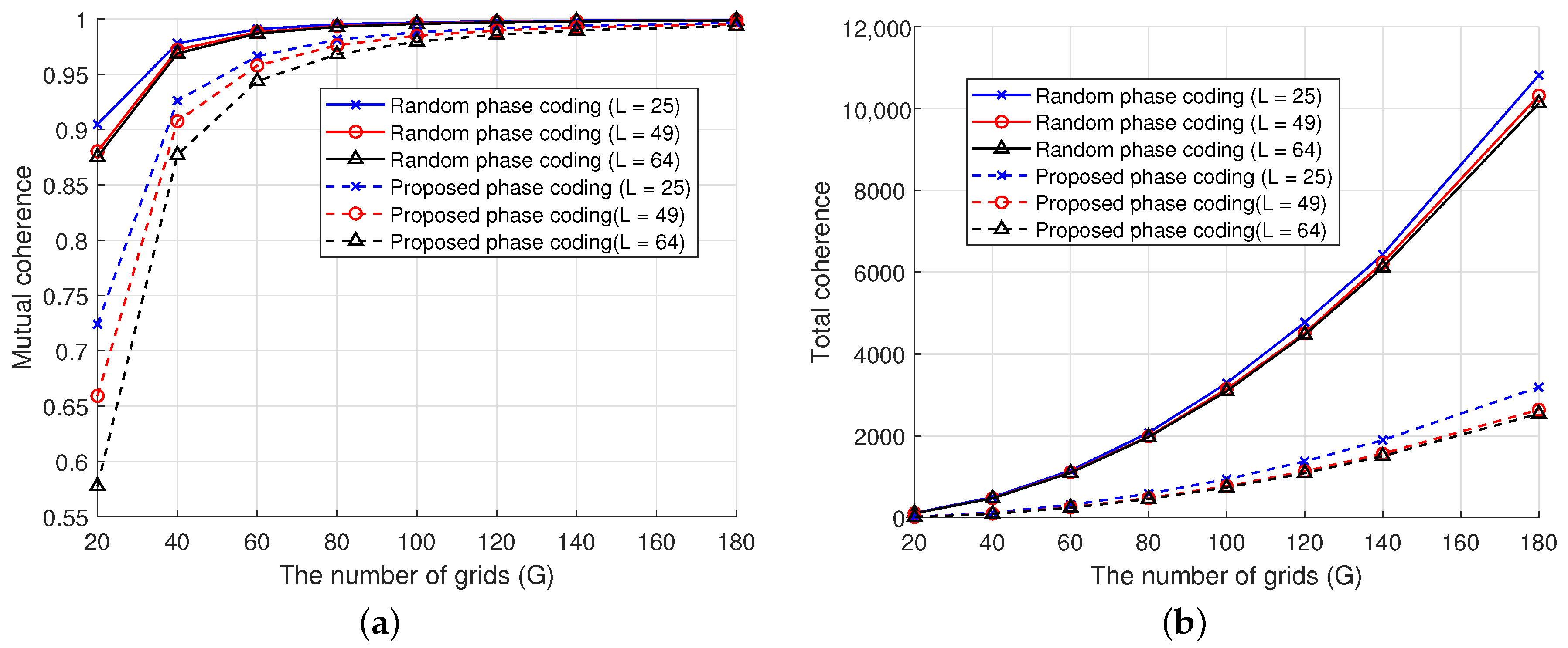
4.2. Validity Analysis

Figure 2 illustrates the element-wise visualization of the normalized Gram matrix of the measurement matrix H ¯ , generated using both the random phase coding matrix and the proposed phase coding design, with the number of coding sequences L = 49 and G = 100 . The ( i , j ) th element of the normalized Gram matrix of H ¯ is calculated with h i H h j / h i 2 h j 2 , where h i and h j are two different columns of H ¯ . It can be observed that under the proposed method, the autocorrelation of each column was significantly stronger than the cross-correlation coefficients, indicating enhanced orthogonality of the measurement matrix.
Figure 3 presents histograms of the off-diagonal elements of the normalized Gram matrix corresponding to both the proposed and the random measurement matrix, where L = 49 and G = 100 . For the random matrix, the off-diagonal elements were more widely distributed, with a significant proportion exceeding 0.2, indicating poor orthogonality. In contrast, the off-diagonal elements of the optimized matrix were concentrated below 0.2, with a peak located near 0. These results demonstrate that the proposed method effectively reduced the magnitude of the off-diagonal elements, reshaped the histogram, and made the distribution more centered around zero. This reduction likely contributed to lower mutual coherence and improved orthogonality of the measurement matrix.
Figure 4 illustrates the trends of mutual coherence and total coherence for the measurement matrix with random phase coding and proposed phase coding as the number of grid points G increased. The grid size G ranged from 20 to 180, with L = 25 , 49 , 64 . The results show that for a given G, the proposed method consistently achieved lower mutual and total coherence compared with the random design, thereby enhancing overall system performance. Additionally, the number of encoding sequences L also affected the coherence; a larger L led to reduced mutual and total coherence.
Figure 5 compares the DOA estimation results obtained using the random phase coding matrix and the proposed phase coding. The number of target angles was set to four, with the parameters L = 49 , G = 100 , and SNR = 0 dB. With the proposed phase coding design, accurate estimation was achieved for all target directions, whereas the random phase coding exhibited noticeable deviations in estimating certain targets. This demonstrates the advantage of the proposed method in multi-target DOA estimation scenarios.

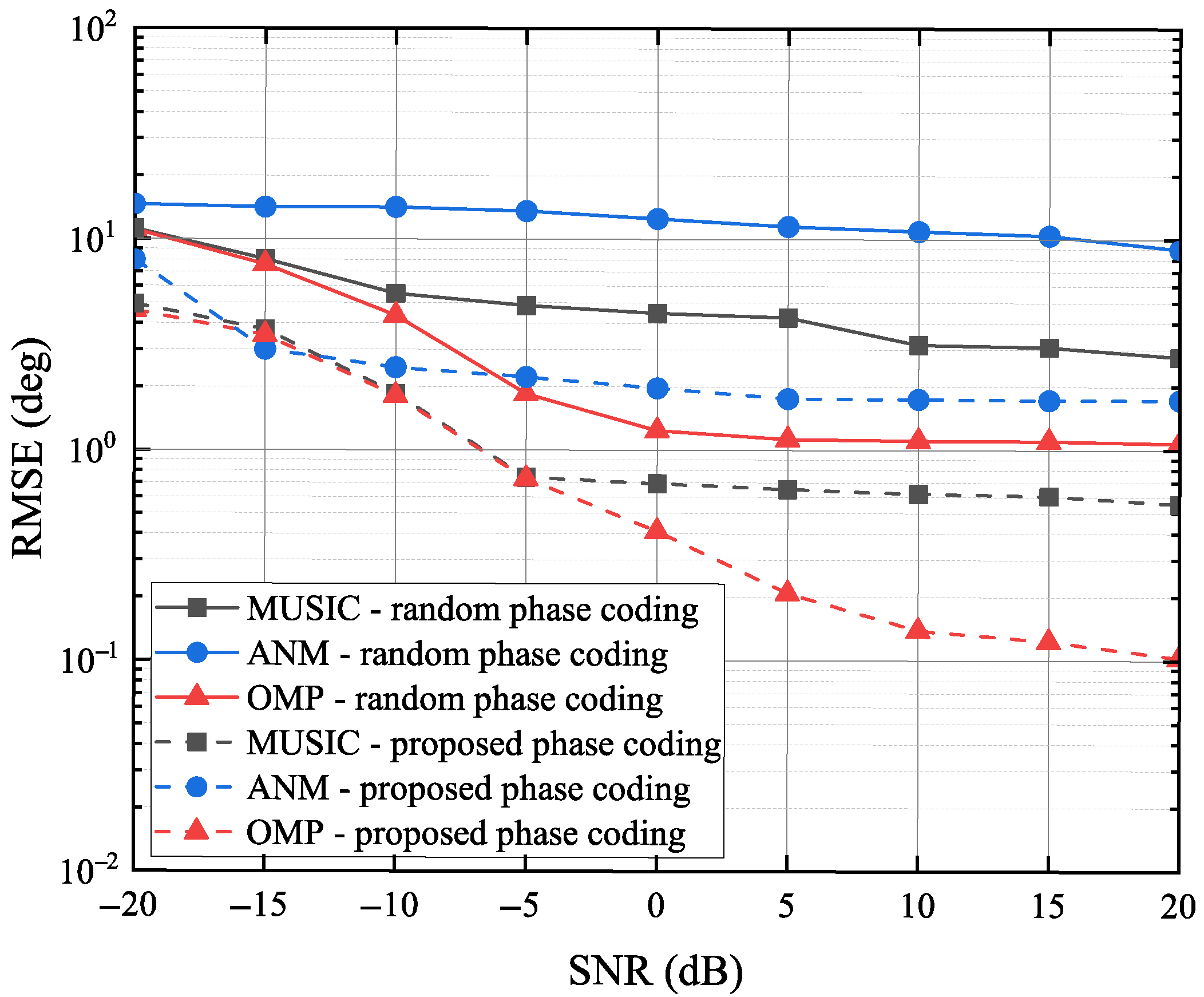
4.3. Performance Analysis Under Different SNRs

Figure 6 compares the RMSE of DOA estimation versus the SNR for three algorithms: OMP, MUSIC, and ANM. Each was evaluated under both the proposed phase coding design and random phase coding. The target angles were set to 4 . 01 ° and 17 . 46 ° , with L = 25 . The simulation results show that the proposed phase coding design yielded the most significant performance improvement for the OMP algorithm. In particular, the RMSE of OMP with the proposed coding was below 1 ° even at an SNR of 5 dB, achieving the best performance among all configurations. Additionally, both MUSIC and ANM also benefited from the proposed coding design, showing noticeable improvements compared with their counterparts using random phase coding.
Figure 7 illustrates the variation in resolution probability with the SNR. The target angles were set to 4 . 01 ° and 17 . 46 ° , with L = 25 . Under identical SNR conditions, the DOA estimation methods with the proposed phase coding exhibited a higher resolution probability than the random phase coding. Notably, the OMP algorithm with the proposed phase coding achieved a resolution probability close to one at an SNR of 5 dB.

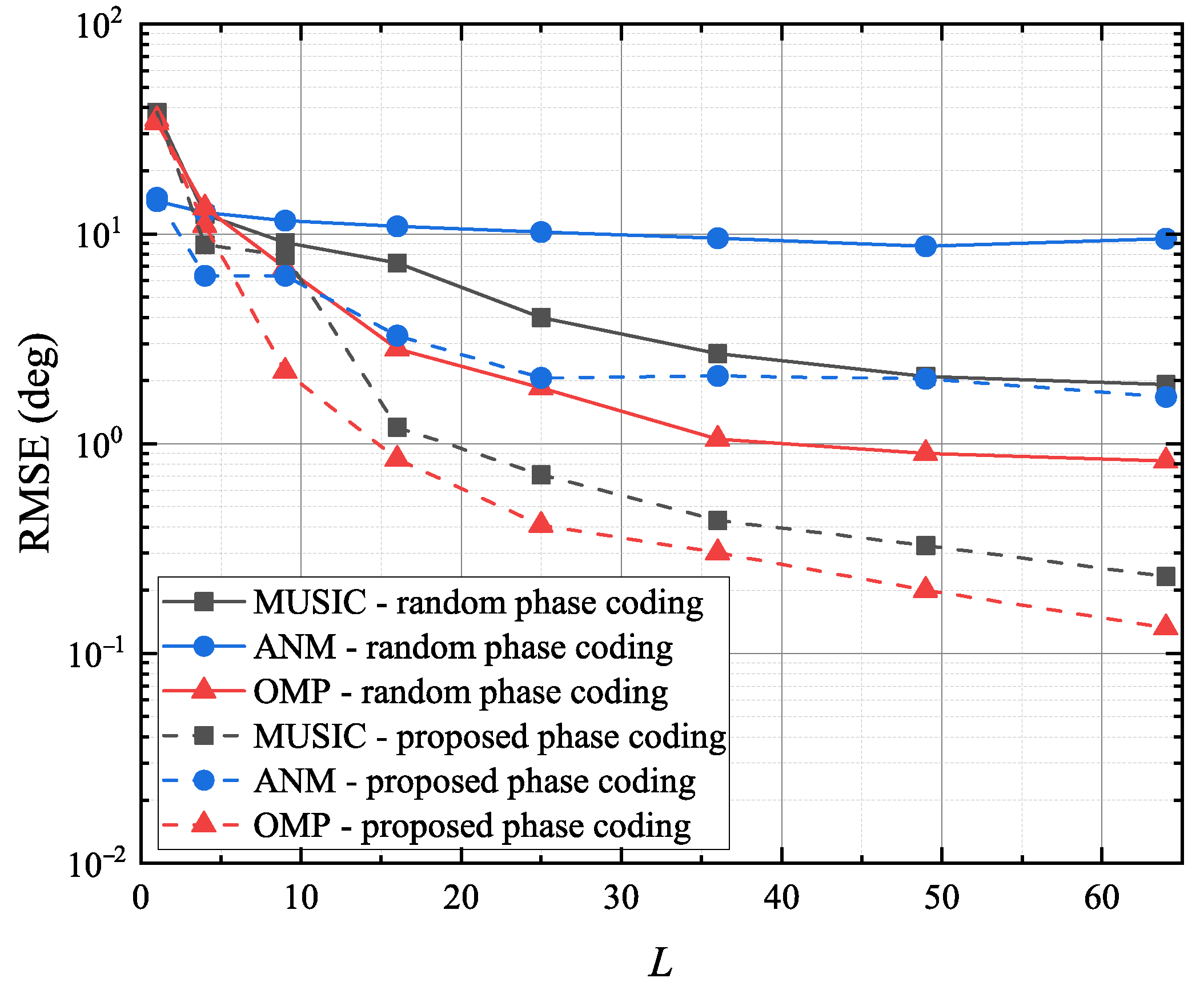
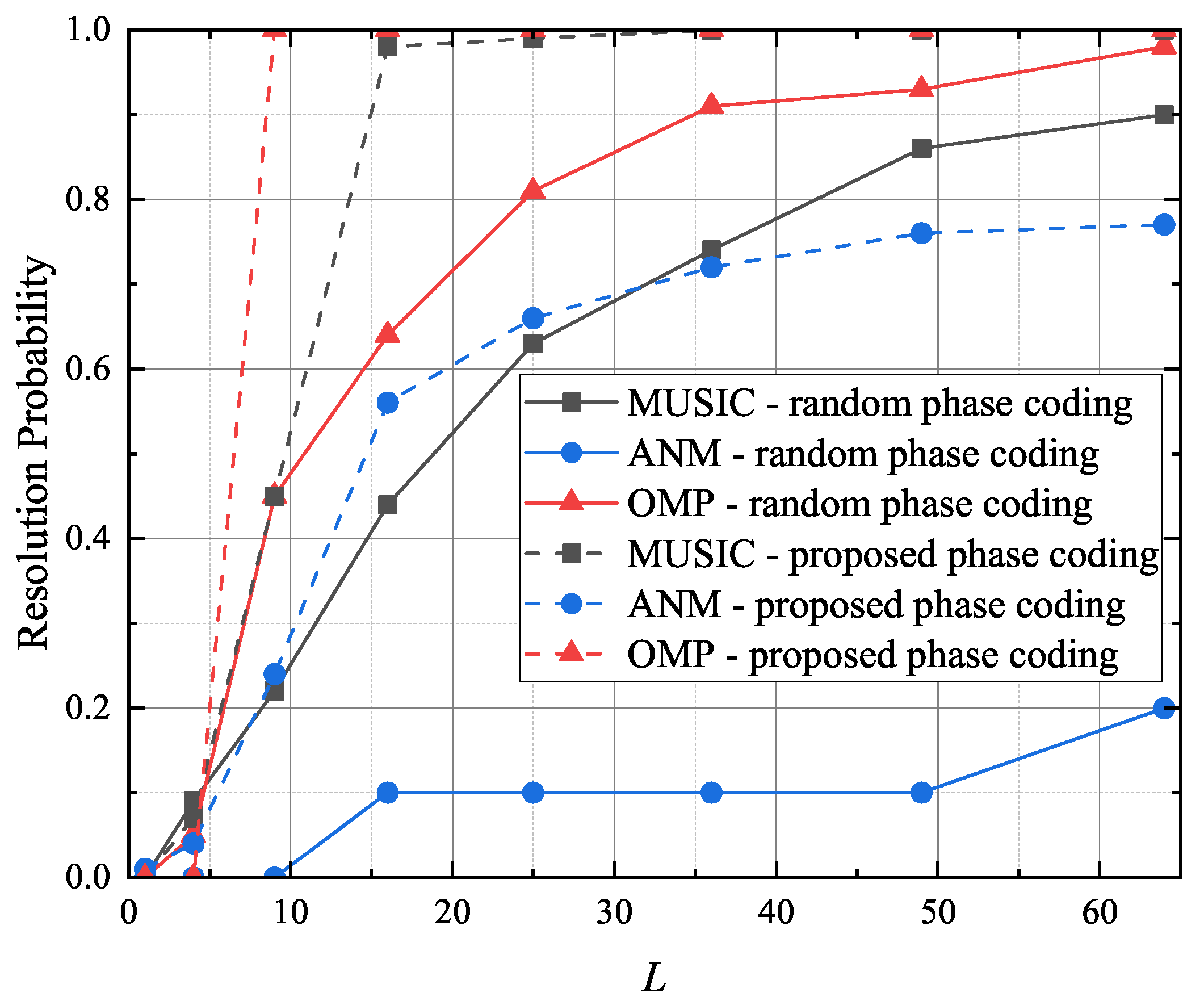
4.4. Performance Analysis Under Different L Values

Figure 8 compares the RMSE performance of the OMP, MUSIC, and ANM algorithms using both random phase coding and the proposed phase coding as the number of coding sequences L varied. The target angles were set to 4 . 01 ° and 17 . 46 ° , and the SNR was fixed at 0 dB. The simulation results indicate that across all values of L, the DOA estimation algorithms using the proposed phase coding consistently achieved lower RMSE values than those using random coding. Notably, when L > 16 , the RMSE of the OMP algorithm with the proposed coding fell below 1 ° , demonstrating its superior estimation accuracy.
Figure 9 illustrates the resolution probability as a function of the number of coding sequences L, with the SNR fixed at 0 dB. Within the range from L = 9 to L = 64 , the OMP algorithm with the proposed phase coding consistently achieved a higher resolution probability than its counterpart using random phase coding. Specifically, at L = 16 , the proposed coding enabled the OMP algorithm to reach a resolution probability close to one, while the random coding approach yielded a significantly lower probability. These results demonstrate that, compared with random coding, the proposed method substantially reduced the required number of coding sequences to achieve high-resolution DOA estimation.

4.5. Performance Analysis Under Different Angles

Figure 10 evaluates the angular resolution probability of DOA estimation over the incident angle range from 60 ° to 60 ° under L = 25 and an SNR of 0 dB. In this simulation, two target angles were considered, corresponding to the values along the x axis and y axis, while the z axis represents the resolution probability for each angle pair. The results show that the proposed phase coding scheme yielded significantly higher resolution probabilities compared with random coding. In particular, the OMP algorithm with the proposed coding maintained a stable and near-perfect resolution probability for any two angles on the selected angle grids separated by more than a certain threshold, demonstrating its superior resolution capability.

5. Conclusions

In this paper, we proposed a phase coding design method for RIS-aided DOA estimation using a single receiving channel. A system model was first established based on an RIS architecture, where a power-based signal model was constructed by averaging the received signals. Based on this model, the DOA estimation problem was transformed into a sparse signal recovery problem in the framework of compressed sensing, where the far-field power radiation pattern of the RIS behaved as the measurement matrix. Then, we derived the decoupled expression of the measurement matrix, which consisted of the phase coding matrix, propagation phase shifts, and array steering matrix. To improve estimation performance, we reformulated the phase coding design task as a total coherence minimization problem. Since direct optimization is non-convex and challenging, we further transformed it into a Frobenius norm minimization problem, aiming to approximate the Gram matrix of the measurement matrix to an identity matrix. Based on this reformulation, a deterministic phase coding strategy was developed using the product of a unitary matrix and a partial Hadamard matrix. The simulation results verified that the proposed phase coding design significantly reduced the DOA estimation error and achieved a higher resolution probability compared with the methods with random phase coding.

Author Contributions

Conceptualization, methodology, software, validation, and writing—original draft, C.H.; supervision, R.Z.; investigation, J.W., B.S., Y.M., C.M. and W.K.; writing—review and editing, R.Z. All authors have read and agreed to the published version of the manuscript.

Funding

This work was supported in part by the Key Laboratory of Intelligent Space TTC&O (Space Engineering University), Ministry of Education under Grant CYK2025-01-12, and in part by the National Natural Science Foundation of China under Grants 62201266, 62301254, and in part by the Natural Science Foundation of Jiangsu Province under Grants BK20210335, BK20230916, and in part by the Fundamental Research Funds for the Central Universities (No. 30925010512, No. 30925010602).

Data Availability Statement

The original contributions presented in this study are included in this article. Further inquiries can be directed to the corresponding author.

Acknowledgments

The authors extend their sincere thanks to the editors and reviewers for their careful reading and fruitful suggestions.

Conflicts of Interest

The authors declare no conflicts of interest.

Appendix A. The Proof of Lemma 1

While denoting Q x = B x W A , Q y = B y W * A * , we have
μ t ( H ¯ ) = m G n = 1 n m G H ¯ ( : , m ) H H ¯ ( : , n ) 2 = m G n = 1 n m G Q x ( : , m ) H Q y ( : , m ) H Q x ( : , n ) Q y ( : , n ) 2 = ( a ) m G n = 1 n m G Q x ( : , m ) H Q x ( : , n ) 2 Q y ( : , m ) H Q y ( : , n ) 2 ( b ) m G n = 1 n m G Q x ( : , m ) H Q x ( : , n ) 2 m G n = 1 n m G Q y ( : , m ) H Q y ( : , n ) 2 ,
where equality (a) follows from the identity ( A B ) ( C D ) = ( A C ) ( B D ) and inequality (b) holds due to the Cauchy—Schwarz inequality.

Appendix B. The Proof of Lemma 2

When d = λ / 2 and the grid division satisfies Equation (24), the mth row of matrix A is
A m , : = [ e j π 1 m 1 , e j π 2 G 1 m 1 , , e j π 2 G G 1 1 m 1 ] .
Based on Equation (A2), the ( m , n ) th element of A A H can be calculated as
A A H m , n = g = 1 G e j π 2 G g 1 1 m n
= G m = n , 0 m n ,
where the second equality is obtained by summing the exponential terms. This means that A A H = G I L x . Meanwhile, W is a diagonal matrix with a unit modulus, and thus we have WW H = I M .

Appendix C. The Proof of Lemma 3

The matrix F x can be decomposed using singular value decomposition as F x = U x Λ x V x H , where U x C L x × L x and V x C L x × L x are unitary matrices, and Λ x C L x × L x is a diagonal matrix containing the singular values of F x , i.e., Λ x = diag δ 1 , , δ L x . Therefore, Equation (27) can be reformulated as
min G M F x F x H I L x F 2 = min G M U x Λ x V x H V x Λ x H U x H I L x F 2 = min G M U x Λ x Λ x H 1 G M I L x U x H F 2 = min Λ x Λ x H 1 G M I L x F 2 .
where the first equality holds due to the singular value decomposition of F x . The remaining steps utilize the unitary invariance of the Frobenius norm and the orthonormality of the SVD components U x and V x , thereby reducing the minimization to a function of the singular values only.
Similarly, the constraint in Equation (27) can be expressed as i = 1 L x δ i 2 = c L x . Thus, the optimization problem in Equation (28) reduces to
min δ i δ i 2 1 G M F 2 s . t . i = 1 L x δ i 2 = c L x .
The solution to Equation (A5) is δ i 2 = c , and Λ x = c I L x . Thus, the optimized solution for Equation (27) is F x opt = c U ¯ x V ¯ x H , where U ¯ x C L x × L x and V ¯ x C L x × L x represent arbitrary unitary matrices.

References

  1. Luo, X.; Lin, Q.; Zhang, R.; Chen, H.; Wang, X.; Huang, M. ISAC—A Survey on Its Layered Architecture, Technologies, Standardizations, Prototypes and Testbeds. IEEE Commun. Surv. Tutor. 2025, 1. [Google Scholar] [CrossRef]
  2. Zhang, R.; Shim, B.; Zhao, H. Downlink Compressive Channel Estimation with Phase Noise in Massive MIMO Systems. IEEE Trans. Commun. 2020, 68, 5534–5548. [Google Scholar] [CrossRef]
  3. Xu, T.; Wang, X.; Huang, M.; Lan, X.; Sun, L. Tensor-Based Reduced-Dimension MUSIC Method for Parameter Estimation in Monostatic FDA-MIMO Radar. Remote Sens. 2021, 13, 3772. [Google Scholar] [CrossRef]
  4. Wu, Y.; Li, C.; Thomas Hou, Y.; Lou, W. A Real-time Super-resolution DoA Estimation Algorithm for Automotive Radar Sensor. IEEE Sens. J. 2024, 24, 37947–37961. [Google Scholar] [CrossRef]
  5. Zhang, T.; Shen, X.; Shang, Z.; Ding, G.; Wu, H.; Qiao, X. An Open-Set Few-Shot Class Incremental Learning Framework for Specific Emitter Identification. IEEE Trans. Cogn. Commun. Netw. 2025, 1. [Google Scholar] [CrossRef]
  6. Zhang, R.; Cheng, L.; Wang, S.; Lou, Y.; Gao, Y.; Wu, W.; Ng, D.W.K. Integrated Sensing and Communication with Massive MIMO: A Unified Tensor Approach for Channel and Target Parameter Estimation. IEEE Trans. Wirel. Commun. 2024, 23, 8571–8587. [Google Scholar] [CrossRef]
  7. Zhang, R.; Cheng, L.; Zhang, W.; Guan, X.; Cai, Y.; Wu, W.; Zhang, R. Channel Estimation for Movable-Antenna MIMO Systems Via Tensor Decomposition. IEEE Wireless Commun. Lett. 2024, 13, 3089–3093. [Google Scholar] [CrossRef]
  8. Schmidt, R. Multiple emitter location and signal parameter estimation. IEEE Trans. Antennas Propag. 1986, 34, 276–280. [Google Scholar] [CrossRef]
  9. Roy, R.; Kailath, T. ESPRIT-estimation of signal parameters via rotational invariance techniques. IEEE Trans. Acoust. Speech Signal Process. 1989, 37, 984–995. [Google Scholar] [CrossRef]
  10. Zhao, W. Research on super resolution angle measurement based on esprit algorithm. J. Phys. Conf. Ser. 2023, 2646, 012014. [Google Scholar] [CrossRef]
  11. Wagner, M.; Park, Y.; Gerstoft, P. Gridless DOA Estimation and Root-MUSIC for Non-Uniform Linear Arrays. IEEE Trans. Signal Process. 2021, 69, 2144–2157. [Google Scholar] [CrossRef]
  12. Liu, S.; Mao, Z.; Zhang, Y.D.; Huang, Y. Rank Minimization-Based Toeplitz Reconstruction for DoA Estimation Using Coprime Array. IEEE Commun. Lett. 2021, 25, 2265–2269. [Google Scholar] [CrossRef]
  13. Chen, P.; Cao, Z.; Chen, Z.; Wang, X. Off-Grid DOA Estimation Using Sparse Bayesian Learning in MIMO Radar with Unknown Mutual Coupling. IEEE Trans. Signal Process. 2019, 67, 208–220. [Google Scholar] [CrossRef]
  14. Zhang, R.; Zhang, J.; Gao, Y.; Zhao, H. Block Bayesian matching pursuit based channel estimation for FDD massive MIMO system. AEU-Int. J. Electron. Commun. 2018, 93, 296–304. [Google Scholar] [CrossRef]
  15. Sun, M.; Wang, Y.; Pan, J. Direction of Arrival Estimation by a Modified Orthogonal Propagator Method with Spline Interpolation. IEEE Trans. Veh. Technol. 2019, 68, 11389–11393. [Google Scholar] [CrossRef]
  16. Fang, J.; Wang, F.; Shen, Y.; Li, H.; Blum, R.S. Super-Resolution Compressed Sensing for Line Spectral Estimation: An Iterative Reweighted Approach. IEEE Trans. Signal Process. 2016, 64, 4649–4662. [Google Scholar] [CrossRef]
  17. Li, Y.; Chi, Y. Off-the-Grid Line Spectrum Denoising and Estimation with Multiple Measurement Vectors. IEEE Trans. Signal Process. 2016, 64, 1257–1269. [Google Scholar] [CrossRef]
  18. Guo, M.; Zhang, Y.D.; Chen, T. DOA estimation using compressed sparse array. IEEE Trans. Signal Process. 2018, 66, 4133–4146. [Google Scholar] [CrossRef]
  19. Zhang, R.; Wu, W.; Chen, X.; Gao, Z.; Cai, Y. Terahertz Integrated Sensing and Communication-Empowered UAVs in 6G: A Transceiver Design Perspective. IEEE Veh. Technol. Mag. 2025, 2–11. [Google Scholar] [CrossRef]
  20. Zhang, R.; Shim, B.; Wu, W. Direction-of-Arrival Estimation for Large Antenna Arrays with Hybrid Analog and Digital Architectures. IEEE Trans. Signal Process. 2022, 70, 72–88. [Google Scholar] [CrossRef]
  21. Ma, Y.; Ma, R.; Lin, Z.; Zhang, R.; Cai, Y.; Wu, W.; Wang, J. Improving Age of Information for Covert Communication with Time-Modulated Arrays. IEEE Internet Things J. 2025, 12, 1718–1731. [Google Scholar] [CrossRef]
  22. Cui, T.J. Microwave metamaterials. Nat. Sci. Rev. 2018, 5, 134–136. [Google Scholar] [CrossRef]
  23. Chen, Z.; Chen, G.; Tang, J.; Zhang, S.; So, D.K.; Dobre, O.A.; Wong, K.K.; Chambers, J. Reconfigurable-Intelligent-Surface-Assisted B5G/6G Wireless Communications: Challenges, Solution, and Future Opportunities. IEEE Commun. Mag. 2023, 61, 16–22. [Google Scholar] [CrossRef]
  24. Abeywickrama, S.; Zhang, R.; Wu, Q.; Yuen, C. Intelligent Reflecting Surface: Practical Phase Shift Model and Beamforming Optimization. IEEE Trans. Commun. 2020, 68, 5849–5863. [Google Scholar] [CrossRef]
  25. Zhang, R.; Chen, G.; Cheng, L.; Guan, X.; Wu, Q.; Wu, W.; Zhang, R. Tensor-based Channel Estimation for Extremely Large-Scale MIMO-OFDM with Dynamic Metasurface Antennas. IEEE Trans. Wirel. Commun. 2025, 1. [Google Scholar] [CrossRef]
  26. Chen, G.; Zhang, R.; Zhang, H.; Miao, C.; Ma, Y.; Wu, W. Energy-Efficient Beamforming for Downlink Multi-User Systems with Dynamic Metasurface Antennas. IEEE Commun. Lett. 2025, 29, 284–288. [Google Scholar] [CrossRef]
  27. Wu, J.; Kim, S.; Shim, B. Energy-Efficient Power Control and Beamforming for Reconfigurable Intelligent Surface-Aided Uplink IoT Networks. IEEE Trans. Wirel. Commun. 2022, 21, 10162–10176. [Google Scholar] [CrossRef]
  28. Wen, F.; Wang, H.; Gui, G.; Sari, H.; Adachi, F. Polarized Intelligent Reflecting Surface Aided 2D-DOA Estimation for NLoS Sources. IEEE Trans. Wirel. Commun. 2024, 23, 8085–8098. [Google Scholar] [CrossRef]
  29. Cui, T.J.; Qi, M.Q.; Wan, X.; Zhao, J.; Cheng, Q.; Lee, K.T.; Lee, J.Y.; Seo, S.; Guo, L.J.; Zhang, Z.; et al. Coding metamaterials, digital metamaterials and programmable metamaterials. Light Sci. Appl. 2014, 3, e213. [Google Scholar] [CrossRef]
  30. Xia, D.; Wang, X.; Han, J.; Xue, H.; Liu, G.; Shi, Y.; Li, L.; Cui, T.J. Accurate 2-D DoA estimation based on active metasurface with nonuniformly periodic time modulation. IEEE Trans. Microw. Theory Technol. 2022, 71, 3424–3435. [Google Scholar] [CrossRef]
  31. Yang, Z.; Chen, P.; Guo, Z.; Ni, D. Low-Cost Beamforming and DOA Estimation Based on One-Bit Reconfigurable Intelligent Surface. IEEE Signal Process. Lett. 2022, 29, 2397–2401. [Google Scholar] [CrossRef]
  32. Chen, G.; Su, X.; He, L.; Guan, D.; Liu, Z. Coherent Signal DOA Estimation Method Based on Space–Time–Coding Metasurface. Remote Sens. 2025, 17, 218. [Google Scholar] [CrossRef]
  33. Lin, M.; Xu, M.; Wan, X.; Liu, H.; Wu, Z.; Liu, J.; Deng, B.; Guan, D.; Zha, S. Single Sensor to Estimate DOA with Programmable Metasurface. IEEE Internet Things J. 2021, 8, 10187–10197. [Google Scholar] [CrossRef]
  34. Wang, J.; Huang, Z.; Xiao, Q.; Li, W.; Li, B.; Wan, X.; Cui, T. High-Precision Direction-of-Arrival Estimations Using Digital Programmable Metasurface. Adv. Intell. Syst. 2022, 4, 2100164. [Google Scholar] [CrossRef]
  35. Chen, P.; Chen, Z.; Zheng, B.; Wang, X. Efficient DOA Estimation Method for Reconfigurable Intelligent Surfaces Aided UAV Swarm. IEEE Trans. Signal Process. 2022, 70, 743–755. [Google Scholar] [CrossRef]
  36. Zheng, Y.; Wang, Q.; Ren, L.; Ma, Z.; Fan, P. RIS Aided Gridless 2D-DOA Estimation via Decoupled Atomic Norm Minimization. IEEE Trans. Veh. Technol. 2024, 73, 15733–15738. [Google Scholar] [CrossRef]
  37. Li, B.; Zhang, S.; Zhang, L.; Shang, X.; Han, C.; Zhang, Y. Robust sensing matrix design for the Orthogonal Matching Pursuit algorithm in compressive sensing. Signal Process. 2025, 227, 109684. [Google Scholar] [CrossRef]
  38. Lee, J.; Gil, G.T.; Lee, Y.H. Channel Estimation via Orthogonal Matching Pursuit for Hybrid MIMO Systems in Millimeter Wave Communications. IEEE Trans. Commun. 2016, 64, 2370–2386. [Google Scholar] [CrossRef]
  39. Ge, X.; Shen, W.; Xing, C.; Zhao, L.; An, J. Training Beam Design for Channel Estimation in Hybrid mmWave MIMO Systems. IEEE Trans. Wirel. Commun. 2022, 21, 7121–7134. [Google Scholar] [CrossRef]
  40. Yu, X.; Shen, J.C.; Zhang, J.; Letaief, K.B. Alternating minimization algorithms for hybrid precoding in millimeter wave MIMO systems. IEEE J. Sel. Top. Signal Process. 2016, 10, 485–500. [Google Scholar] [CrossRef]
  41. Donoho, D. Compressed sensing. IEEE Trans. Inf. Theory. 2006, 52, 1289–1306. [Google Scholar] [CrossRef]
  42. Duarte, M.F.; Eldar, Y.C. Structured Compressed Sensing: From Theory to Applications. IEEE Trans. Signal Process. 2011, 59, 4053–4085. [Google Scholar] [CrossRef]
  43. Cai, T.T.; Wang, L. Orthogonal Matching Pursuit for Sparse Signal Recovery with Noise. IEEE Trans. Inf. Theory. 2011, 57, 4680–4688. [Google Scholar] [CrossRef]
Figure 1. System model for RIS-aided DOA estimation with a single receiving channel.
Remotesensing 17 02394 g001
Figure 2. The normalized Gram matrix of the measurement matrix H ¯ . (a) Random phase coding. (b) Proposed phase coding.
Remotesensing 17 02394 g002
Figure 3. The histogram of the off-diagonal elements of the normalized Gram matrix of the measurement matrix H ¯ . (a) Random phase coding. (b) Proposed phase coding.
Remotesensing 17 02394 g003
Figure 4. Mutual coherence and total coherence versus the number of grids G. (a) Mutual coherence. (b) Total coherence.
Remotesensing 17 02394 g004
Figure 5. DOA estimation results with 4 different targets.
Remotesensing 17 02394 g005
Figure 6. RMSE versus SNR.
Remotesensing 17 02394 g006
Figure 7. Resolution probability versus SNR.
Remotesensing 17 02394 g007
Figure 8. RMSE versus the number of coding sequences.
Remotesensing 17 02394 g008
Figure 9. Resolution probability versus the number of coding sequences.
Remotesensing 17 02394 g009
Figure 10. Resolution probability versus two arbitrary angles. (a) MUSIC with random phase coding. (b) MUSIC with proposed phase coding. (c) OMP with random phase coding. (d) OMP with proposed phase coding.
Remotesensing 17 02394 g010
Table 1. Notations.
Table 1. Notations.
NotationDescription
A * the complex conjugate of a matrix A
A T the transpose of a matrix A
A H the complex conjugate transpose of a matrix A
tr( A )the trace of a matrix A
diag( a )the diagonal matrix with elements in vector a as the diagonals
E ( x ( t ) ) the mathematical expectation of a function x ( t )
A B the Kronecker product of two matrices A and B
A B the Khatri–Rao product of two matrices A and B
| | A | | F the Frobenius norm of a matrix A
| | a | | 2 the l 2 -norm of a vector a
| a | the absolute value of a scalar a
I M the identity matrix of dimensions M × M
Disclaimer/Publisher’s Note: The statements, opinions and data contained in all publications are solely those of the individual author(s) and contributor(s) and not of MDPI and/or the editor(s). MDPI and/or the editor(s) disclaim responsibility for any injury to people or property resulting from any ideas, methods, instructions or products referred to in the content.

