Unmanned Aerial Vehicle-Based RGB Imaging and Lightweight Deep Learning for Downy Mildew Detection in Kimchi Cabbage

Abstract

Downy mildew is a highly destructive fungal disease that significantly reduces both the yield and quality of kimchi cabbage. Conventional detection methods rely on manual scouting, which is labor-intensive and prone to subjectivity. This study proposes an automated detection approach using RGB imagery acquired by an unmanned aerial vehicle (UAV), integrated with lightweight deep learning models for leaf-level identification of downy mildew. To improve disease feature extraction, Simple Linear Iterative Clustering (SLIC) segmentation was applied to the images. Among the evaluated models, Vision Transformer (ViT)-based architectures outperformed Convolutional Neural Network (CNN)-based models in terms of classification accuracy and generalization capability. For late-stage disease detection, DeiT-Tiny recorded the highest test accuracy (0.948) and macro F1-score (0.913), while MobileViT-S achieved the highest diseased recall (0.931). In early-stage detection, TinyViT-5M achieved the highest test accuracy (0.970) and macro F1-score (0.918); however, all models demonstrated reduced diseased recall under early-stage conditions, with DeiT-Tiny achieving the highest recall at 0.774. These findings underscore the challenges of identifying early symptoms using RGB imagery. Based on the classification results, prescription maps were generated to facilitate variable-rate pesticide application. Overall, this study demonstrates the potential of UAV-based RGB imaging for precision agriculture, while highlighting the importance of integrating multispectral data and utilizing domain adaptation techniques to enhance early-stage disease detection.

1. Introduction

Kimchi cabbage (Brassica rapa pekinensis) is a widely cultivated leafy vegetable in East Asia, particularly in South Korea, where it serves as a key ingredient in the preparation of kimchi, a traditional fermented food. However, its yield and quality are significantly threatened by downy mildew (Peronospora parasitica), a fungal disease that thrives in cold, humid conditions. Early symptoms appear as yellow, angular lesions on the upper leaf surface, which later become necrotic, and are accompanied by white mycelial growth on the abaxial leaf surface [1]. Currently, downy mildew detection in kimchi cabbage primarily relies on manual field scouting, a labor-intensive and subjective process. Conventional disease management strategies often involve broad-spectrum pesticide applications, which increase production costs and environmental risks. Therefore, developing an efficient, cost-effective, and accurate disease detection system is crucial for precision agriculture and sustainable crop management.

Unmanned aerial vehicles (UAVs) equipped with remote sensing technologies have revolutionized plant disease detection by enabling large-scale, high-throughput crop monitoring [2]. UAV-mounted sensors, including hyperspectral, multispectral, infrared, and RGB cameras, capture valuable spectral and spatial information for plant disease assessment [3]. Among these, hyperspectral imaging offers fine spectral resolution, enabling precise differentiation between healthy and diseased plants based on their unique spectral signatures [4,5,6]. For instance, Kuswidiyanto et al. effectively employed UAV-based hyperspectral imaging to detect downy mildew in kimchi cabbage [7]. However, the high cost of hyperspectral sensors, along with significant data acquisition, storage, and processing demands, limits their adoption, particularly for small- and medium-sized farms [8,9]. Multispectral imaging, which focuses on specific bands such as red-edge (RE) and near-infrared (NIR), offers a more accessible alternative but still requires specialized and expensive sensors. Infrared imaging can detect variations in leaf temperature associated with physiological stress, such as water deficiency or disease; however, its direct applicability to downy mildew detection remains limited [10]. In contrast, RGB imaging is the most accessible and cost-effective option for large-scale crop monitoring, leveraging color, canopy structure, and texture for disease identification [11,12]. Despite its advantages, RGB imaging lacks spectral depth, making early-stage disease detection challenging due to subtle visual symptoms and background noise [13]. Addressing these limitations using advanced machine learning techniques is critical for improving detection accuracy.

Convolutional Neural Networks (CNNs) are among the earliest deep learning architectures applied to image classification and have demonstrated strong capabilities in extracting local and hierarchical features from images (Figure 1a). Their effectiveness has established them as a foundational technique in agricultural image analysis and plant disease detection [14,15,16]. However, due to their reliance on local receptive fields, CNNs are inherently limited in capturing global contextual information across the entire image. This limitation can hinder their performance in tasks that require integrating spatially dispersed or semantically related features [17,18].

To overcome these limitations, Vision Transformers (ViTs), introduced by Dosovitskiy et al. in 2020 [19], have emerged as a powerful alternative for image analysis tasks. Unlike CNNs, ViTs divide images into fixed-size patches and process them as sequences of tokens using self-attention mechanisms (Figure 1b). This architecture enables ViTs to model long-range dependencies and capture global contextual information more effectively. On large-scale classification benchmarks such as ImageNet, ViTs have demonstrated competitive or superior performance to that of CNNs when trained on sufficiently large datasets. Due to their strong global modeling capability, ViTs show significant potential for plant disease detection in complex field environments characterized by variable lighting, occlusion, and heterogeneous backgrounds. However, the deployment of ViTs in practical agricultural monitoring is constrained by their high computational demands and reliance on large annotated datasets. To address these issues, recent studies have focused on developing lightweight transformer-based models and hybrid architectures that integrate the strengths of both ViTs and CNNs. Notable examples include MobileViT and TinyViT [20,21], which achieve a favorable balance between classification accuracy and computational efficiency. These models are particularly well suited for UAV-based crop disease detection using RGB imagery.

Segmentation plays a pivotal role in UAV-based disease detection by defining the level of analysis [22]. Traditional plant-level segmentation classifies diseases at the whole-plant level, typically requiring large-scale cropping areas for sufficient data collection. However, this method frequently involves image downscaling, potentially obscuring disease symptoms and reducing classification accuracy. In contrast, leaf-level segmentation improves detection performance by dividing individual plants into multiple leaf samples, thereby increasing the number of training samples while preserving fine-grained disease features [23]. This approach enhances both classification accuracy and generalizability across diverse datasets.

This study aimed to develop an efficient UAV-based framework for detecting downy mildew in kimchi cabbage using cost-effective RGB imaging combined with deep learning techniques. The specific objectives were to (1) establish a UAV-based disease detection pipeline incorporating leaf-level segmentation; (2) train lightweight CNN- and ViT-based models for the automated identification of downy mildew symptoms; (3) evaluate and compare model performance, with particular attention to generalizability across different image acquisition dates; and (4) generate prescription maps to support precision disease management.

The main contributions of this study are as follows: (1) a tile-wise processing and SLIC-based leaf segmentation approach specifically designed for UAV-derived orthomosaic images, enabling fine-grained disease detection; (2) deployment and comparative analysis of lightweight CNN and ViT models optimized for UAV deployment constraints, achieving a balance between classification accuracy and inference efficiency; and (3) integration of classification outputs into prescription map generation, providing adaptable zoning strategies for practical disease management in the field.

2. Materials and Methods

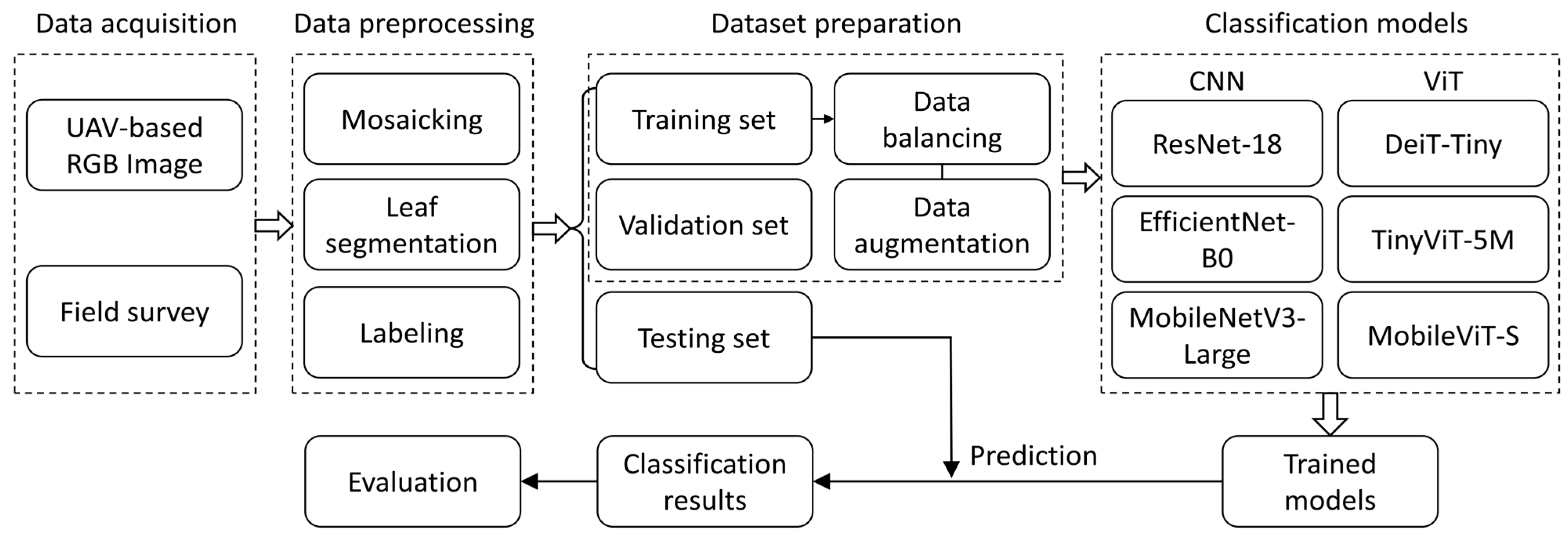
2.1. Overall Workflow

The overall workflow of this study is illustrated in Figure 2, comprising five key stages: data acquisition, preprocessing, dataset preparation, model training, and performance evaluation. Each stage was meticulously designed to improve the accuracy and efficiency of downy mildew detection in kimchi cabbage using UAV-based RGB imagery and lightweight deep learning models.

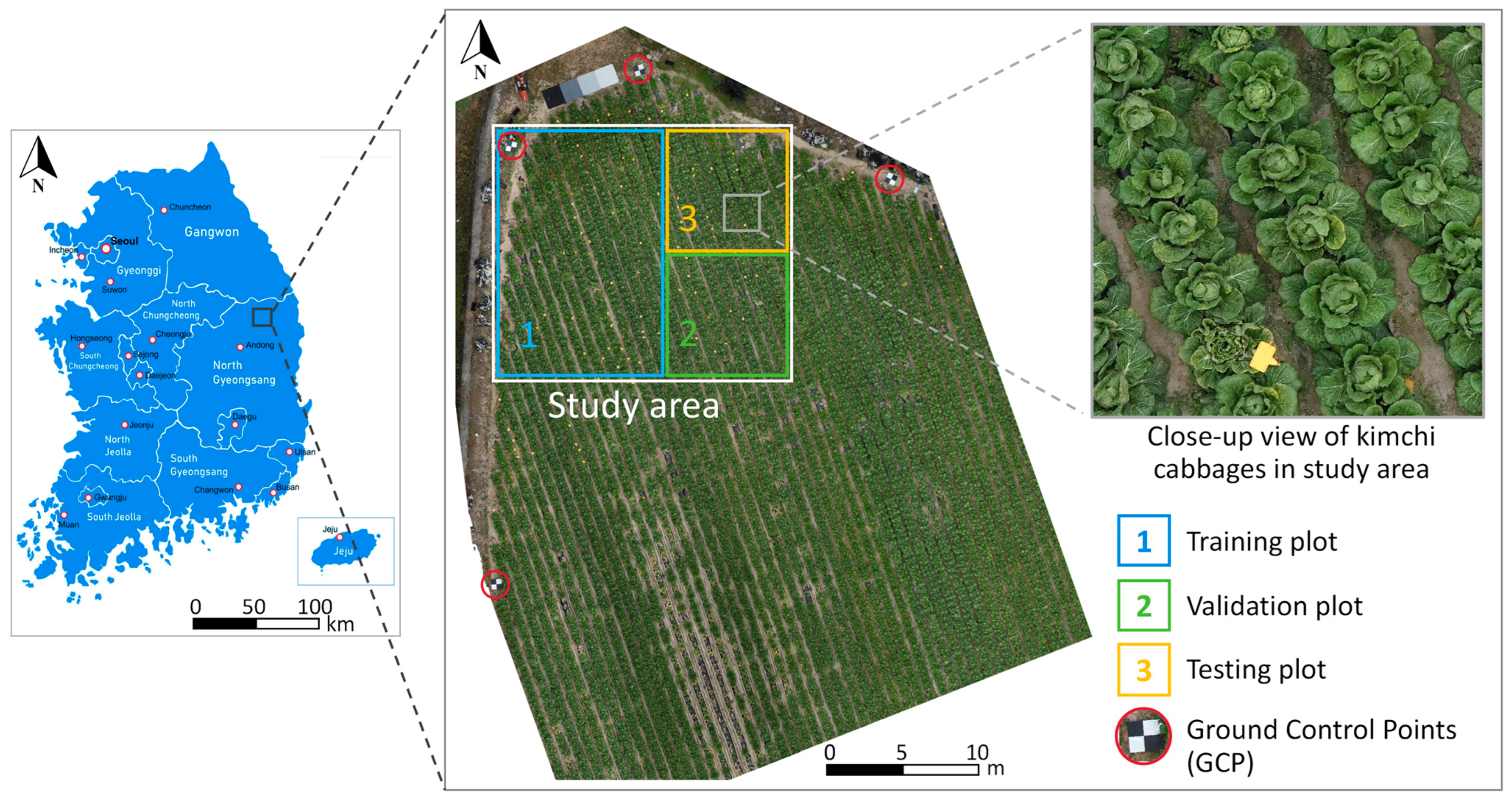
2.2. Study Area and Site Description

As illustrated in Figure 3, the dataset was collected in autumn 2023 from an experimental kimchi cabbage field located in Bonghwa County, South Korea. Sowing occurred in late August, and although general pesticides were applied, no fungicides specifically targeting downy mildew were used to allow for natural disease progression.

To ensure robust model evaluation, the field was strategically divided into training, validation, and test plots, as depicted in the plot schematic. Data acquisition took place between 18 and 25 October, capturing both early-stage and advanced symptoms of downy mildew. Persistent rainfall in mid-October accelerated disease development, with early symptoms (small yellow or yellow-green spots) first observed on 18 October. By 25 October, the disease had progressed significantly, forming widespread, rough-textured yellow lesions.

For model evaluation, images acquired on 25 October were used for model training and testing, while data collected on 18 October were reserved for cross-date validation to assess the model’s generalization performance across different disease stages.

2.3. Data Acquisition

2.3.1. UAV-Based Aerial Imaging

As shown in Figure 4a, a Matrice 300 RTK UAV (DJI, Shenzhen, China) equipped with a Zenmuse P1 RGB camera (DJI, Shenzhen, China; 8192 × 5460 pixels, full-frame CMOS) was deployed for aerial imaging, capturing high-resolution spatial details crucial for accurate disease detection.

The UAV operated at an altitude of 20 m above ground level with a constant speed of 1.83 m/s, achieving a ground sample distance of 0.25 cm per pixel. To ensure uniform image coverage, the flight path was planned using UgCS v4.9 (SPH Engineering, Riga, Latvia) in a grid-based survey mode, maintaining a 75% forward and side overlap.

Georeferencing accuracy was enhanced using the UAV’s onboard real-time kinematic (RTK) module, supplemented by four ground control points (GCPs) for improved spatial precision. The aerial survey was conducted between 1:00 p.m. and 2:00 p.m. local time under diffuse lighting conditions, as the surrounding mountains partially obstructed direct sunlight. This setup minimized surface glare and leaf shadowing, thereby improving symptom visibility in the RGB imagery. By reducing excessive reflectance and shading artifacts, this approach preserved spectral and textural details essential for accurate disease detection.

2.3.2. Field Survey

Prior to the UAV flight, a plant pathology expert conducted a field survey, manually identifying cabbage leaves exhibiting downy mildew symptoms and marking them with yellow indicators, as illustrated in Figure 4b. Due to the highly transmissible nature of downy mildew, a single marker was used to designate an affected area when multiple adjacent cabbages exhibited symptoms. Detailed records were maintained to ensure precise sample annotation, thereby providing a reliable reference for dataset construction and enabling robust model training and validation.

2.4. Data Preprocessing

2.4.1. Image Mosaicking

Aerial images were processed using Agisoft Metashape (Agisoft LLC, St. Petersburg, Russia) to generate an orthomosaic of the experimental cabbage field. Approximately 300 images were stitched together and georeferenced using the UAV’s onboard RTK module and GCPs, achieving centimeter-level positional accuracy and radiometric consistency.

To facilitate segmentation and annotation, the orthomosaic was further processed using a Python-based script, which divided it into 3000 × 3000-pixel tiles. This tiling approach enabled the large-scale orthomosaic to be processed in manageable segments, reducing computational load and preventing memory overflow during processing. The selected tile size was well suited for visualizing leaf-level features on standard computer screens, thereby supporting accurate segmentation and annotation. The resulting dataset was partitioned into 12 tiles for training, 4 tiles for validation, and 4 tiles for testing, ensuring a balanced data distribution for model development and evaluation.

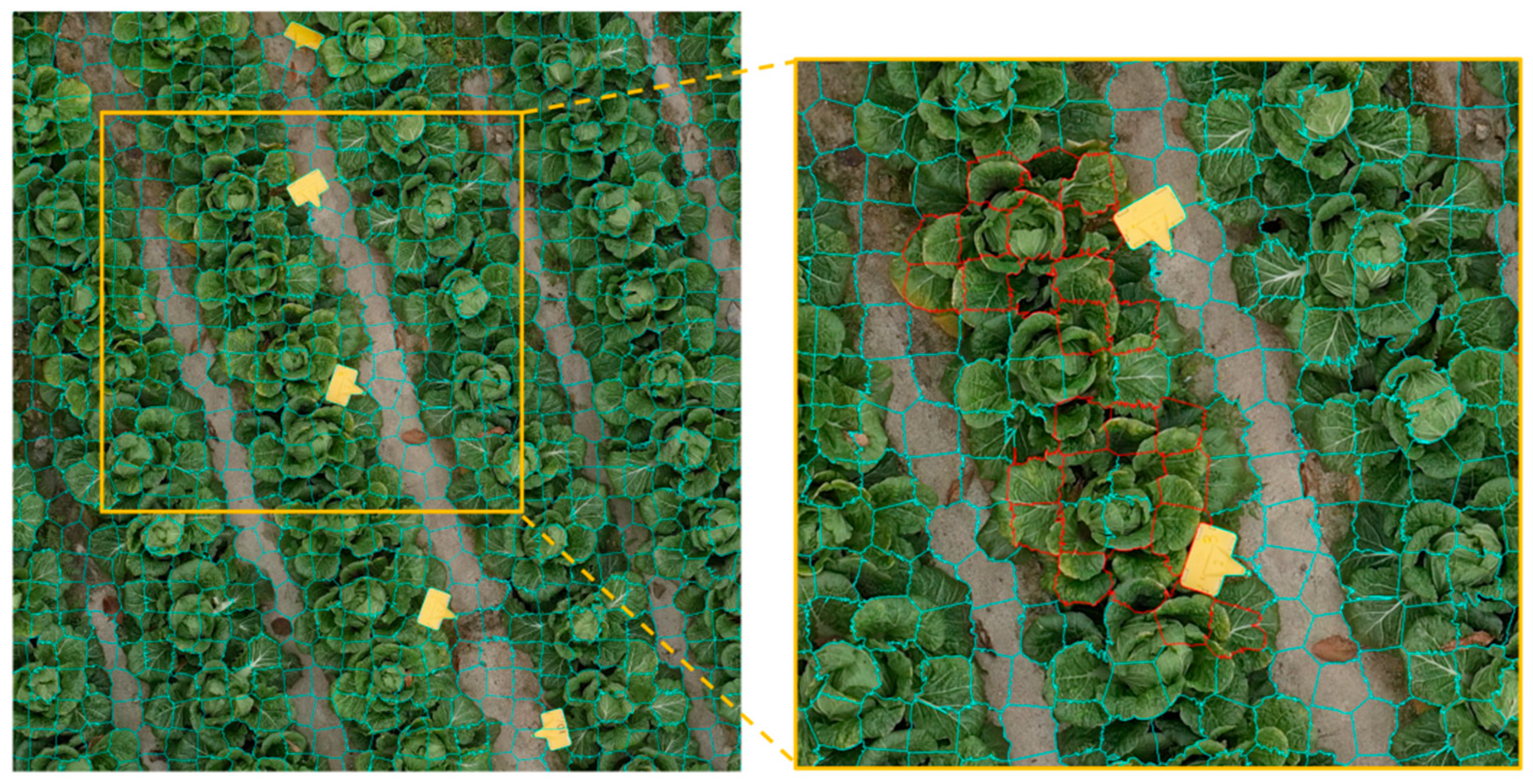
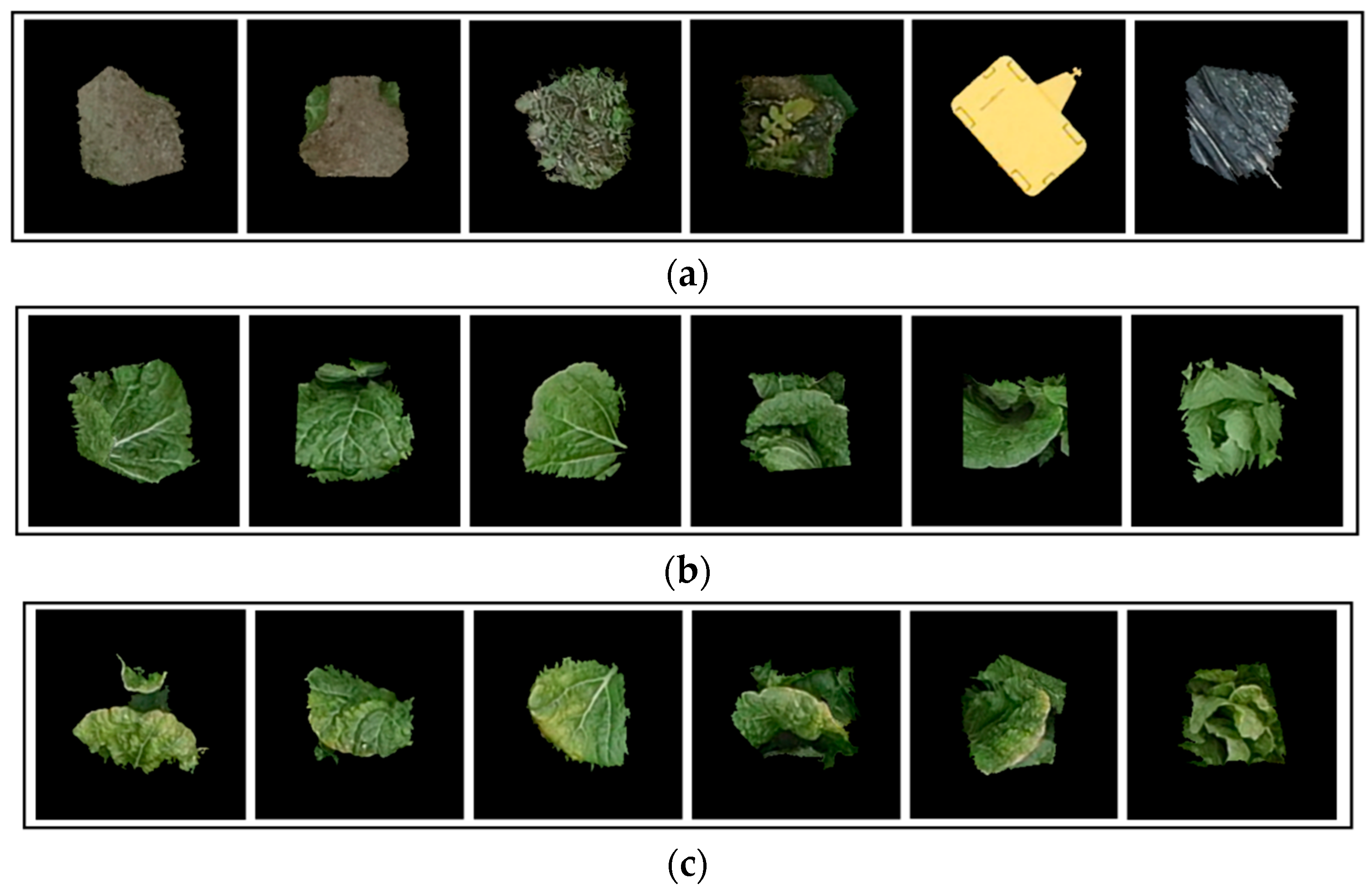
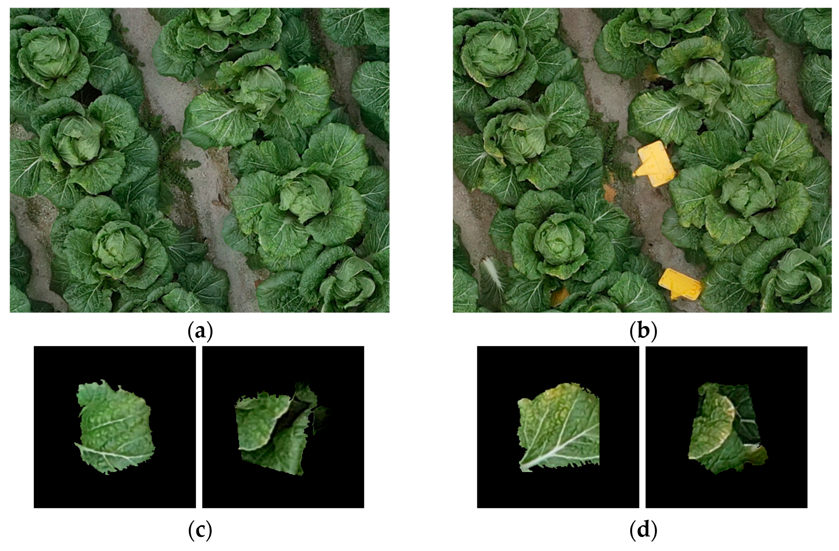
2.4.2. Image Segmentation and Labeling

This study employed Simple Linear Iterative Clustering (SLIC) for superpixel segmentation, a computationally efficient technique particularly suitable for large-scale UAV image processing [24,25]. SLIC enables fine-grained, leaf-level segmentation, thereby enhancing disease classification accuracy [7,26]. The algorithm was implemented in Python using the scikit-image library. For each 3000 × 3000-pixel tile, SLIC segmentation was applied with empirically optimized parameters: num_segments = 900 and compactness = 50. A num_segments value of 900 produced superpixels that closely approximated the size of individual cabbage leaves and effectively delineated inter-row background areas. The compactness parameter—controlling the trade-off between color similarity and spatial proximity—was set to 50 to preserve leaf boundaries while minimizing over-segmentation in shaded or low-contrast regions. These segmented regions were then embedded into 224 × 224 black square patches to ensure compatibility with the input size required for deep learning models. The chosen parameters also enhanced inter-row background delineation, improving sample visibility and ensuring precise labeling of background samples.

To enhance labeling accuracy, a Python-based interactive annotation interface was developed to enable manual selection of diseased samples, as illustrated in Figure 5, with affected regions highlighted in red. Following the initial labeling, a plant pathology expert conducted a verification process to refine the annotations, ensuring precise categorization into three distinct classes (Figure 6): (a) background, (b) healthy leaves, and (c) diseased leaves. This rigorous annotation process ensured high-quality dataset generation, thereby optimizing classification accuracy for deep learning model training and evaluation.

2.5. Dataset Preparation

2.5.1. Dataset Partitioning

The dataset was divided into training, validation, and test sets based on separate field plots to ensure spatial data independence. Prior research has demonstrated that spatially independent dataset partitioning offers a more accurate evaluation of model performance in UAV-based disease detection than random sampling, as it better reflects real-world deployment conditions [27]. Given the resource-intensive nature of field data collection and the study’s objective of developing a low-cost disease detection method, the dataset was constrained by the size of the study area and the limited availability of diseased samples. To optimize model training and evaluation, the dataset was partitioned as follows: 60% for training, 20% for validation, and 20% for testing, based on the total area.

Model training was performed using data collected on 25 October, when disease symptoms were more pronounced, resulting in a higher number of diseased samples. The test set comprised data from both 18 October and 25 October, enabling the assessment of the model’s generalization capability across different time points. This partitioning was particularly crucial for evaluating the model’s ability to detect early-stage symptoms, which were visually subtle on 18 October.

2.5.2. Data Balancing and Augmentation

The dataset exhibited significant class imbalance, with healthy leaves constituting the majority. Even in the 25 October dataset, where symptoms were more evident, the training set included only 610 diseased samples, yielding an overall class distribution of approximately 2:9:1 (background:healthy:diseased). Imbalanced training data can cause models to be biased toward the majority class, thereby reducing recall for diseased samples and impairing both detection accuracy and generalization capability [28].

To address this issue, a data balancing strategy was applied to the training set. Healthy samples were downsampled, while diseased samples underwent augmentation and upsampling, resulting in a final class distribution of 1:2:1 (background:healthy:diseased) (

Table 1. Sample distribution across dataset partitions, with the training set balanced at a 1:2:1 ratio, while the validation and test sets retained their original distribution.

Class	Original Training Set	Balanced Training Set	Validation Set	Testing Set (25 October)	Testing Set (18 October)
Background	1520	1520	767	860	819
Healthy	6742	3040	2367	2211	2458
Diseased	610	1520	258	321	115
Total	8872	6080	3392	3392	3392

). This approach aligns with the recommendations of Buda et al., who emphasized that upsampling should mitigate class imbalance, while the optimal downsampling ratio should be carefully determined to maintain model stability and prevent overfitting [29].

To enhance data diversity and improve model generalization, diseased samples were subjected to data augmentation techniques, including random rotation, flipping, and color jittering. These transformations helped reduce overfitting by exposing the model to a wider range of variations in disease appearance [30]. Meanwhile, the validation and test sets remained unbalanced to reflect real-world conditions, where class distributions are inherently skewed, thereby enabling a more realistic evaluation of model performance [31].

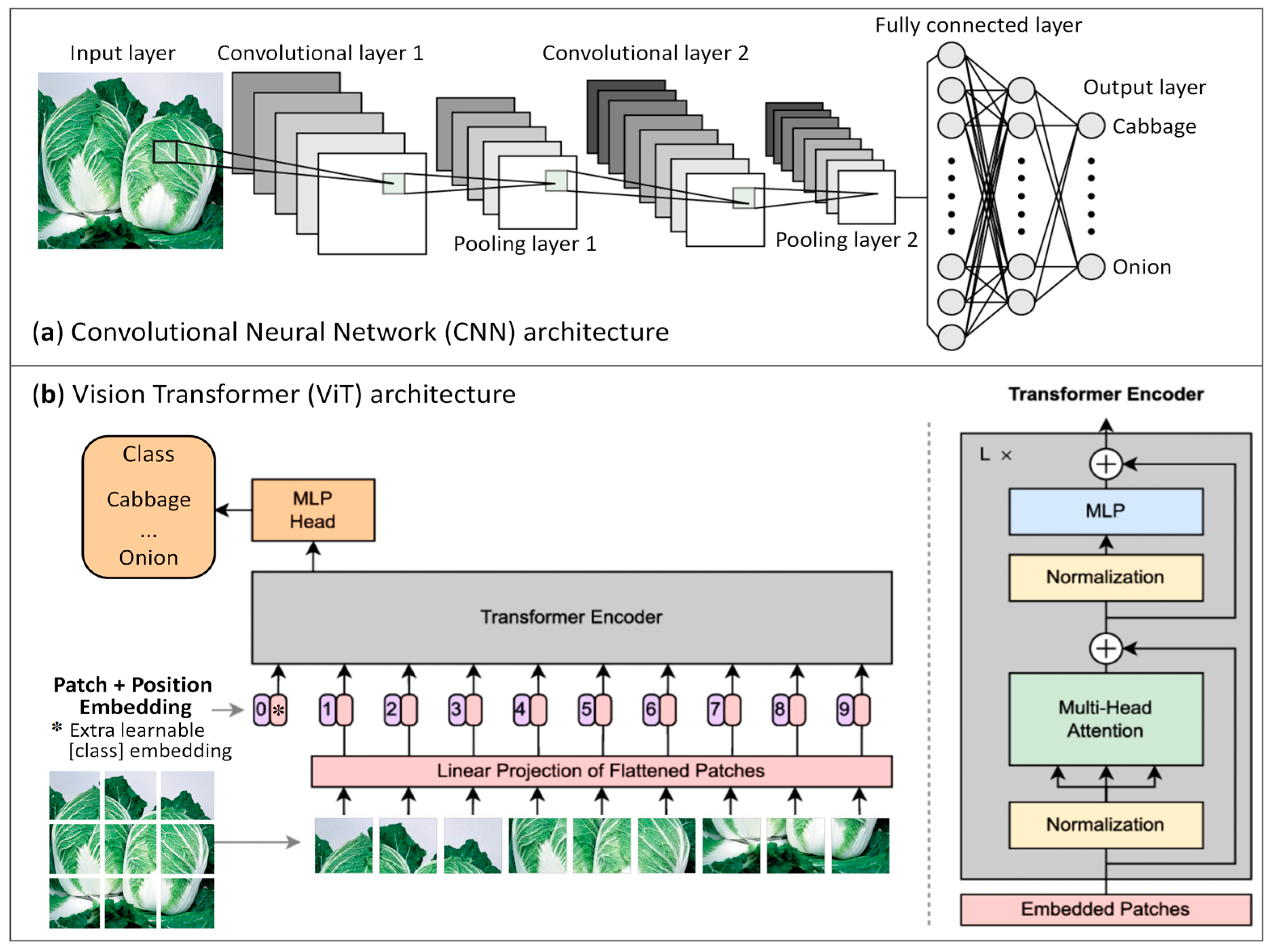
2.6. Lightweight CNN and ViT Models

To detect downy mildew in kimchi cabbage, six deep learning models were developed and evaluated, including one baseline CNN and five lightweight architectures. The baseline model was ResNet-18, while the lightweight models included two CNN-based architectures (EfficientNet-B0 and MobileNetV3-Large) and three compact ViT-based models (DeiT-Tiny, TinyViT-5M, and MobileViT-S). As shown in

Table 2. Comparison of key parameters and structural characteristics of the six models.

Model	Type	Parameters (M)	FLOPs 1 (G)	Input Size (Pixels)	Structural Features
ResNet-18	CNN	11.7	1.8	224 × 224	Residual blocks, 3 × 3 conv, and skip connections
EfficientNet-B0	CNN	5.3	0.39	224 × 224	MBConv 2, SE 3, and compound scaling
MobileNetV3-Large	CNN	5.4	0.22	224 × 224	Inverted residuals, SE, and h-swish 4
DeiT-Tiny	ViT	5.7	1.3	224 × 224	Patch embedding, transformer blocks, class token, and distillation
TinyViT-5M	ViT (Hybrid) 5	5.4	1.3	224 × 224	Local convolution, hierarchical transformer, and window attention
MobileViT-S	ViT (Hybrid)	5.6	1.1	224 × 224	Convolution blocks, transformer blocks, and local–global fusion

¹ FLOPs, Floating Point Operations. ² MBConv, Mobile Bottleneck Convolution. ³ SE, Squeeze-and-Excitation. ⁴ h-swish, hard-swish. ⁵ ViT (Hybrid), a hybrid model combining ViT and CNN modules.

, ResNet-18 contains about 11.7 million parameters, whereas the lightweight models range from approximately 5.3 to 5.7 million parameters, allowing for a relatively balanced comparison of classification performance across diverse architectural paradigms.

ResNet-18 utilizes residual blocks composed of stacked 3 × 3 convolutions, preceded by an initial 7 × 7 convolution with a stride of 2. All convolutional layers are followed by ReLU activation and Batch Normalization [32]. This residual design effectively addresses the vanishing gradient problem, enhancing both training stability and feature extraction. EfficientNet-B0 employs a compound scaling strategy based on MBConv blocks with 3 × 3 and 5 × 3 kernels, Swish activation, and squeeze-and-excitation (SE) modules (reduction ratio = 0.25). This configuration jointly optimizes network depth, width, and resolution, providing an excellent balance between computational efficiency and accuracy [33]. MobileNetV3-Large integrates 5 × 5 depthwise separable convolutions with SE modules and h-swish activation (channel reduction ratio = 4), achieving lightweight performance through neural architecture search [34]. Among the transformer-based models, DeiT-Tiny is a compact ViT architecture that utilizes 16 × 16 patch embeddings, GELU activation, and knowledge distillation to enhance training efficiency, particularly on limited datasets [35]. TinyViT-5M adopts a hierarchical structure to balance performance and efficiency: (1) a 4 × 4 convolutional stem for local feature extraction, (2) transformer blocks with shifted-window attention (window size = 7) for global context modeling, and (3) progressive channel reduction from 64 to 32 dimensions, maintaining a total of 5.7 million parameters [21]. MobileViT-S features a hybrid architecture combining: (1) CNN-based local feature extraction via 3 × 3 convolutions with ReLU activation, and (2) transformer blocks with patch-based self-attention and GELU activation. In this step, CNN-derived features are flattened into patch tokens, allowing the model to preserve the local inductive bias of CNNs while leveraging the global receptive field of transformers [20].

2.7. Model Training and Experimental Setup

Hyperparameter selection plays a critical role in training deep learning models, as it significantly influences convergence behavior and overall performance. To ensure a fair comparison across the four models, preliminary experiments were conducted to determine optimal hyperparameter settings. Based on these results, a uniform set of hyperparameters was applied across all models to maintain consistent training conditions. The batch size was set to 64, with an initial learning rate of 0.0001. A learning rate scheduler reduced the learning rate by a factor of 10⁻¹ every five epochs, facilitating gradual parameter refinement and improving convergence stability.

Each model was trained for 50 epochs with an early stopping mechanism (patience = 12 epochs) to prevent overfitting by halting training when validation performance plateaued. Furthermore, regularization techniques, including a dropout rate of 0.3 and weight decay of 1 × 10⁻⁴ were employed to enhance generalization, effectively reducing overfitting while preserving model stability and robustness.

The training was conducted using Python 3.8.10 with PyTorch 1.12.1, an open-source deep learning framework. All experiments were executed on a 64-bit Windows 11 Pro workstation equipped with an Intel Core i9 processor (3.20 GHz) and an NVIDIA RTX A5000 GPU (24 GB VRAM). The software environment was configured with CUDA 11.6 and cuDNN 8.4 for efficient GPU-accelerated training. Additionally, NumPy, OpenCV, and scikit-learn were utilized for data preprocessing and evaluation.

2.8. Model Evaluation

Model evaluation was performed using both predictive performance and computational efficiency metrics to ensure a comprehensive assessment of classification accuracy and deployment feasibility.

The predictive performance of the model was assessed using multiple classification metrics, including accuracy (Equation (1)), precision (Equation (2)), recall (Equation (3)), F1-score (Equation (4)), and macro-averaged F1-score (Equation (5)). These metrics provided a balanced assessment across all classification categories, capturing both overall and class-specific performances. A normalized confusion matrix was also employed to visualize class-wise prediction distributions and identify misclassification patterns. The formulas for the predictive performance metrics are provided below.

$$\mathrm{A}\mathrm{c}\mathrm{c}\mathrm{u}\mathrm{r}\mathrm{a}\mathrm{c}\mathrm{y}={\displaystyle \frac{\mathrm{T}\mathrm{P}+\mathrm{T}\mathrm{N}}{\mathrm{T}\mathrm{P}+\mathrm{T}\mathrm{N}+\mathrm{F}\mathrm{P}+\mathrm{F}\mathrm{N}}}$$

(1)

$$\mathrm{P}\mathrm{r}\mathrm{e}\mathrm{c}\mathrm{i}\mathrm{s}\mathrm{i}\mathrm{o}\mathrm{n}={\displaystyle \frac{\mathrm{T}\mathrm{P}}{\mathrm{T}\mathrm{P}+\mathrm{F}\mathrm{P}}}$$

(2)

$$\mathrm{R}\mathrm{e}\mathrm{c}\mathrm{a}\mathrm{l}\mathrm{l}={\displaystyle \frac{\mathrm{T}\mathrm{P}}{\mathrm{T}\mathrm{P}+\mathrm{F}\mathrm{N}}}$$

(3)

$$\mathrm{F}1={\displaystyle \frac{2\times \mathrm{P}\mathrm{r}\mathrm{e}\mathrm{c}\mathrm{i}\mathrm{s}\mathrm{i}\mathrm{o}\mathrm{n}\times \mathrm{R}\mathrm{e}\mathrm{c}\mathrm{a}\mathrm{l}\mathrm{l}}{\mathrm{P}\mathrm{r}\mathrm{e}\mathrm{c}\mathrm{i}\mathrm{s}\mathrm{i}\mathrm{o}\mathrm{n}+\mathrm{R}\mathrm{e}\mathrm{c}\mathrm{a}\mathrm{l}\mathrm{l}}}$$

(4)

$$\mathrm{M}\mathrm{a}\mathrm{c}\mathrm{r}\mathrm{o}-\mathrm{F}1={\displaystyle \frac{1}{\mathrm{N}}}\sum _{\mathrm{i}=1}^{\mathrm{N}}{\mathrm{F}1}_{\mathrm{i}}$$

(5)

where TP, TN, FP, and FN denote true positives, true negatives, false positives, and false negatives, respectively.

To assess computational efficiency, two key performance indicators were measured: total training time and inference time on the test set. Total training time was recorded to evaluate the feasibility of model optimization and retraining, while inference time was measured to determine the model’s suitability for real-time deployment in UAV-based disease detection. These metrics provided valuable insights into the trade-offs between model accuracy and deployment efficiency, supporting practical implementation in precision agriculture settings.

The evaluation was conducted in two stages. First, model performance was assessed using the 25 October dataset, which featured more pronounced disease symptoms, allowing for the evaluation of detection accuracy under clearly visible infection conditions. Next, a cross-date evaluation was performed using the 18 October dataset to examine the model’s generalization capability across different time points and its effectiveness in identifying early-stage symptoms, which were less visually distinct. This two-stage approach provided a comprehensive assessment of the model’s effectiveness in detecting both late-stage and early-stage infections.

3. Results

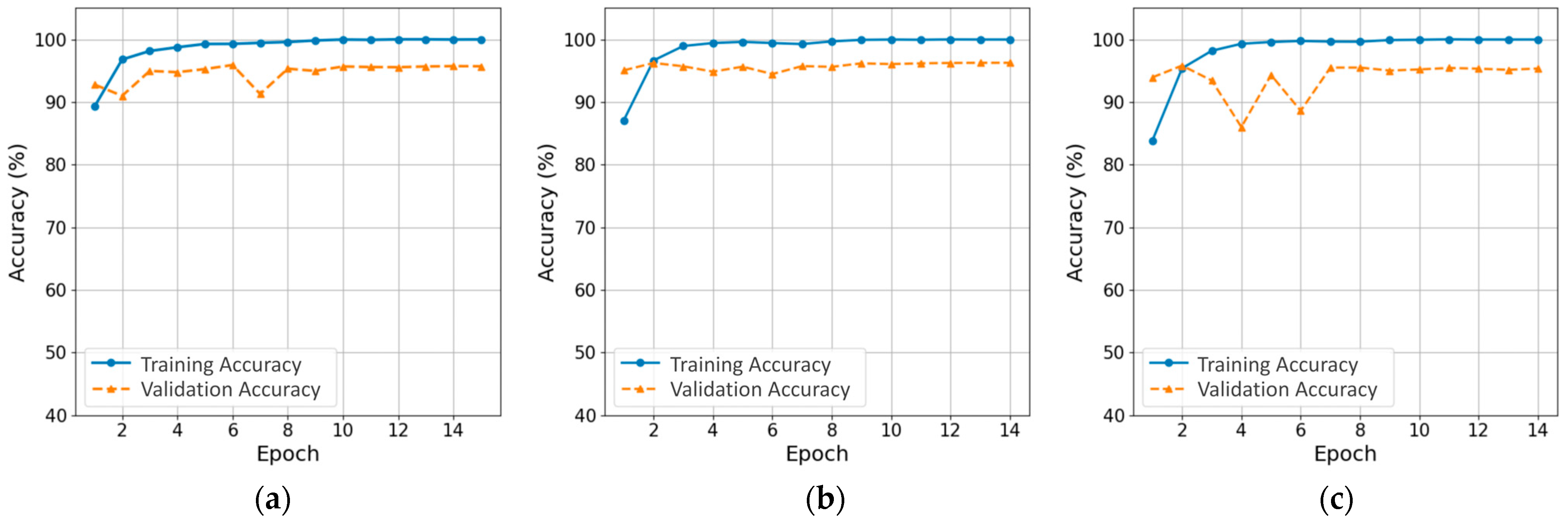
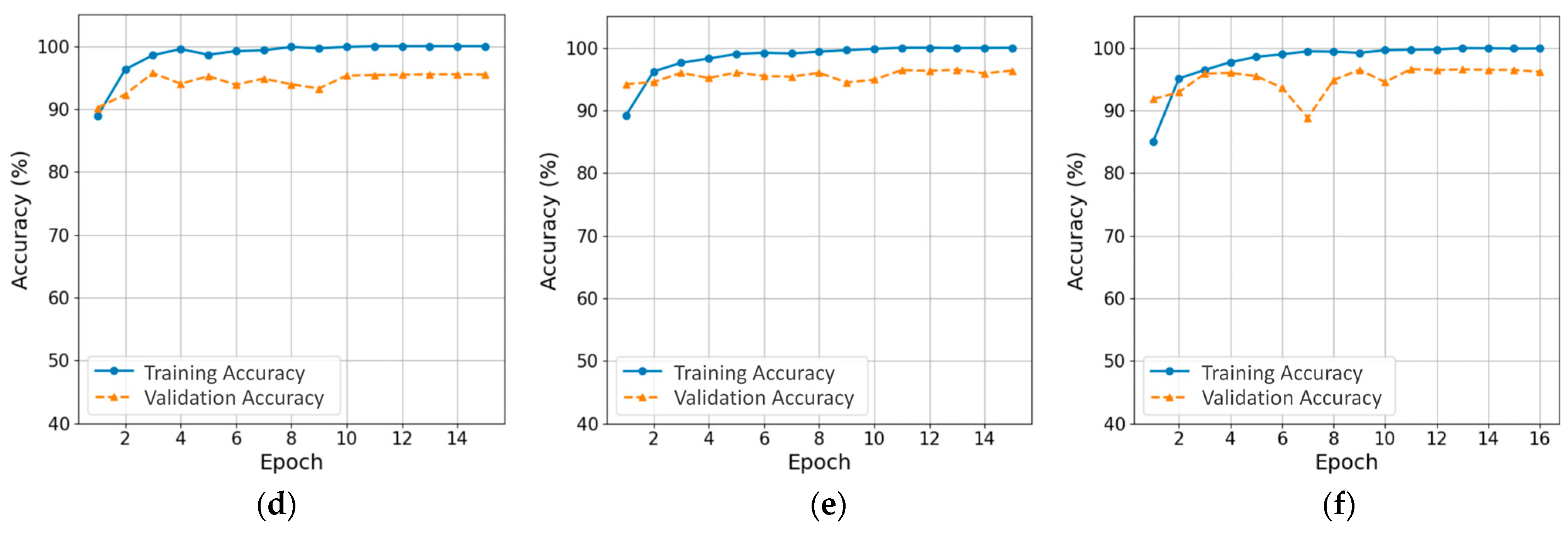
3.1. Training Process and Computational Efficiency of CNN and ViT Models

Figure 7 presents the training and validation accuracy curves for all six models. Each model was trained under identical experimental conditions, utilizing the same dataset, hyperparameters, and training protocol (an initial learning rate of 0.0001, a batch size of 64, and a learning rate decay by a factor of 10 every five epochs). The training process spanned a maximum of 50 epochs, with an early stopping mechanism (patience = 12 epochs) implemented to mitigate overfitting and enhance generalization performance. To ensure fair and reproducible comparisons across architectures, a fixed random seed was used during training. Among six candidate seeds (0–5), seed 2 was selected based on stable training behavior observed across all models. Under this setting, early stopping was consistently triggered between epochs 14 and 16. The resulting performance metrics closely aligned with the median values from multiple trials, indicating that the selected runs were representative and minimally affected by stochastic variation.

Under this configuration, ResNet-18 triggered early stopping at epoch 15, while EfficientNet-B0 and MobileNetV3-Large converged slightly earlier at epoch 14. Among the transformer-based models, DeiT-Tiny and TinyViT-5M completed training at epoch 15, and MobileViT-S at epoch 16. Notably, MobileNetV3-Large exhibited a sharp drop in validation accuracy during epochs 2–4 (Figure 7c), potentially due to (1) transient instability in its SE layers during initial feature calibration and (2) delayed gradient stabilization in its inverted residual blocks. However, this early-phase volatility subsided by epoch 7, reflecting the model’s capacity for self-regulation. These results indicate that even hybrid and transformer-based architectures exhibited stable and consistent convergence behavior under the shared training configuration. As shown in

Table 3. Performance evaluation of each model on the 25 October test set.

Model	Epochs	Training Time (s)	Inference Time (s)	Test Accuracy	Precision (Diseased)	Recall (Diseased)	F1-Score (Diseased)	Macro F1-Score
ResNet-18	15	111.70	1.53	0.936	0.658	0.897	0.759	0.896
EfficientNet-B0	14	176.79	2.09	0.941	0.704	0.882	0.783	0.904
MobileNetV3-Large	14	105.83	1.25	0.941	0.710	0.826	0.764	0.899
DeiT-Tiny	15	140.83	1.78	0.948	0.731	0.882	0.799	0.913
TinyViT-5M	15	225.15	2.59	0.947	0.704	0.903	0.791	0.911
MobileViT-S	16	326.15	3.49	0.946	0.691	0.931	0.793	0.912

, all six models achieved competitive computational and inference efficiency, although some differences in training and inference times were observed. MobileNetV3-Large emerged as the most efficient model, completing training in 105.83 s and achieving an inference time of only 1.25 s. ResNet-18 and DeiT-Tiny also demonstrated favorable efficiency, with training times of 111.70 s and 140.83 s, and inference times of 1.53 s and 1.78 s, respectively. Notably, despite its transformer-based structure, DeiT-Tiny maintained high efficiency due to its compact architecture and data-efficient training. In contrast, EfficientNet-B0 required a longer training duration of 176.79 s and an inference time of 2.09 s, reflecting its more complex scaling strategy. TinyViT-5M and MobileViT-S recorded the longest training durations (225.15 s and 326.15 s) and inference times (2.59 s and 3.49 s), likely attributed to the additional computational overhead associated with integrating convolutional layers and transformer modules.

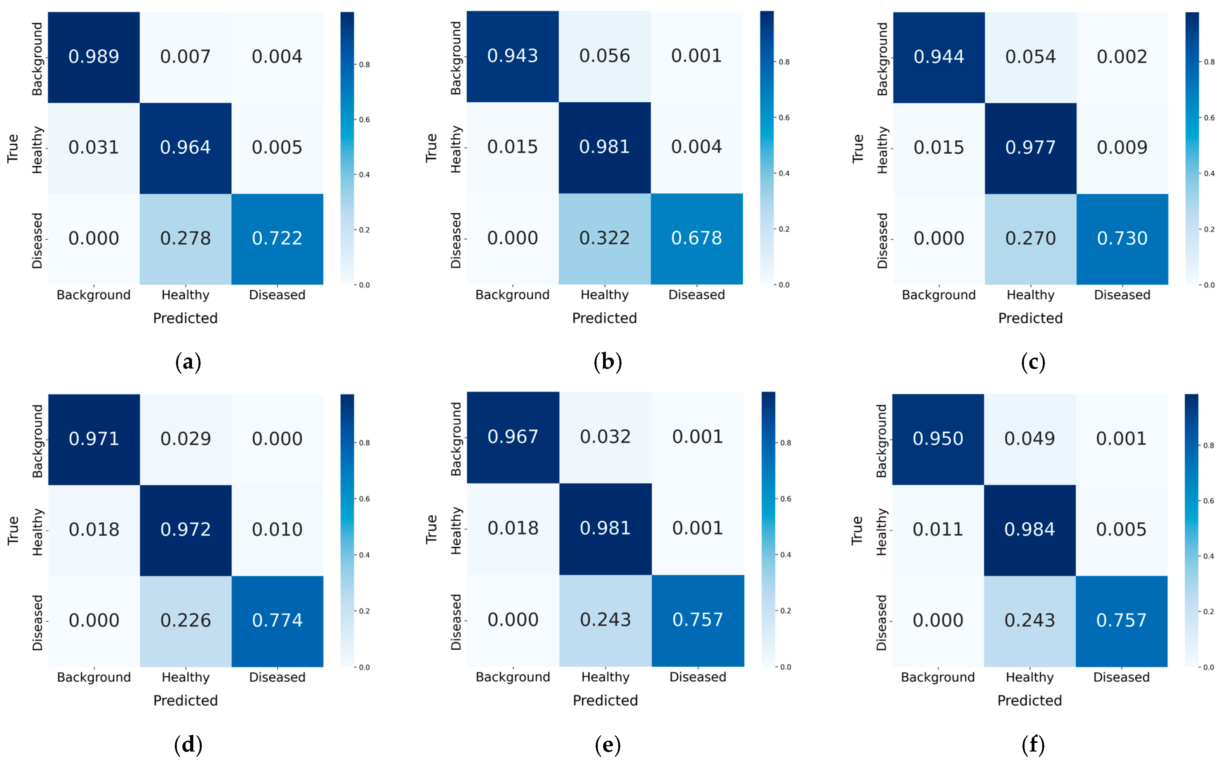
3.2. Classification Performance and Cross-Date Generalization

As presented in Table 3 and Figure 8, all models demonstrated strong classification performance on the 25 October test set, with overall accuracies ranging from 0.936 (ResNet-18) to 0.948 (DeiT-Tiny). This date coincided with a period when disease symptoms were more visually prominent, likely contributing to the high prediction accuracies observed across models. For the diseased class, MobileViT-S achieved the highest recall (0.931) and a strong F1-score (0.793), followed by TinyViT-5M (recall: 0.903; F1-score: 0.791), DeiT-Tiny (recall: 0.882; F1-score: 0.799), ResNet-18 (recall: 0.897; F1-score: 0.759), EfficientNet-B0 (recall: 0.882; F1-score: 0.783), and MobileNetV3-Large (recall: 0.826; F1-score: 0.764). Regarding the macro-averaged F1-score, which accounts for classification balance across all categories, DeiT-Tiny achieved the highest score (0.913), closely followed by MobileViT-S (0.912) and TinyViT-5M (0.911). These results suggest that all models effectively distinguished between infected, healthy, and background samples under conditions where disease symptoms were clearly visible. Notably, the transformer-based and hybrid models—particularly MobileViT-S and TinyViT-5M—achieved higher recall and F1-scores compared with their CNN-based counterparts. This performance indicates their enhanced capability to capture complex visual features, highlighting their potential advantages in accurately detecting diseases when visual cues are pronounced.

To assess each model’s generalization capability across different time periods, a cross-date evaluation was conducted using the 18 October test set, which corresponds to the early to mid-stage of downy mildew development when visible symptoms were less pronounced and more difficult to detect. As shown in

Table 4. Performance evaluation of each model on the 18 October test set.

Model	Inference Time (s)	Test Accuracy	Precision (Diseased)	Recall (Diseased)	F1-Score (Diseased)	Macro F1-Score
ResNet-18	1.34	0.962	0.847	0.722	0.779	0.901
EfficientNet-B0	2.12	0.961	0.867	0.678	0.761	0.895
MobileNetV3-Large	1.42	0.960	0.785	0.730	0.757	0.893
DeiT-Tiny	1.88	0.965	0.781	0.774	0.777	0.904
TinyViT-5M	2.64	0.970	0.927	0.757	0.829	0.918
MobileViT-S	3.57	0.968	0.870	0.757	0.809	0.915

and Figure 9, all models maintained high overall classification accuracies, ranging from 0.960 to 0.970. However, recall for the diseased class declined compared with the 25 October test set, reflecting the increased difficulty of identifying early-stage infections. Among the CNN-based models, ResNet-18 recorded the highest recall (0.722) with an F1-score of 0.779, followed by MobileNetV3-Large (recall: 0.730; F1-score: 0.757) and EfficientNet-B0 (recall: 0.678; F1-score: 0.761). In contrast, the transformer-based and hybrid models—TinyViT-5M and MobileViT-S—achieved higher recall (0.757) and strong F1-scores (0.829 and 0.809, respectively), while DeiT-Tiny demonstrated moderate performance (recall: 0.774; F1-score: 0.777). These findings indicate that, although all models exhibited reduced effectiveness in detecting early-stage symptoms, transformer-based hybrid architectures—particularly TinyViT-5M and MobileViT-S—provided more stable and robust performance across the dates. Their consistent recall and F1-scores highlight their potential for accurate early-stage disease detection under visually complex field conditions. Further improvements may be achieved through advanced data augmentation strategies or the incorporation of multimodal input to enhance feature representation.

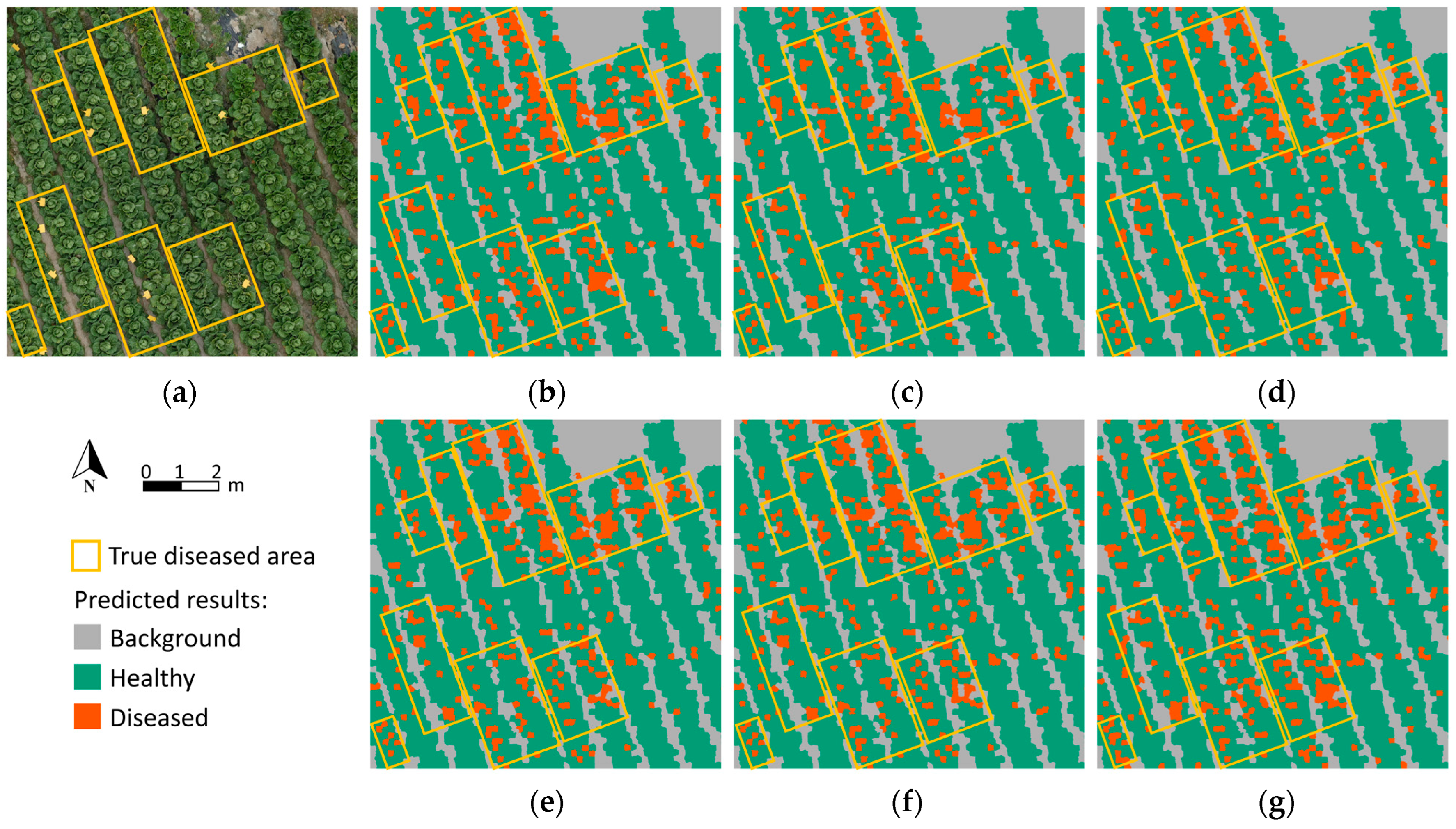
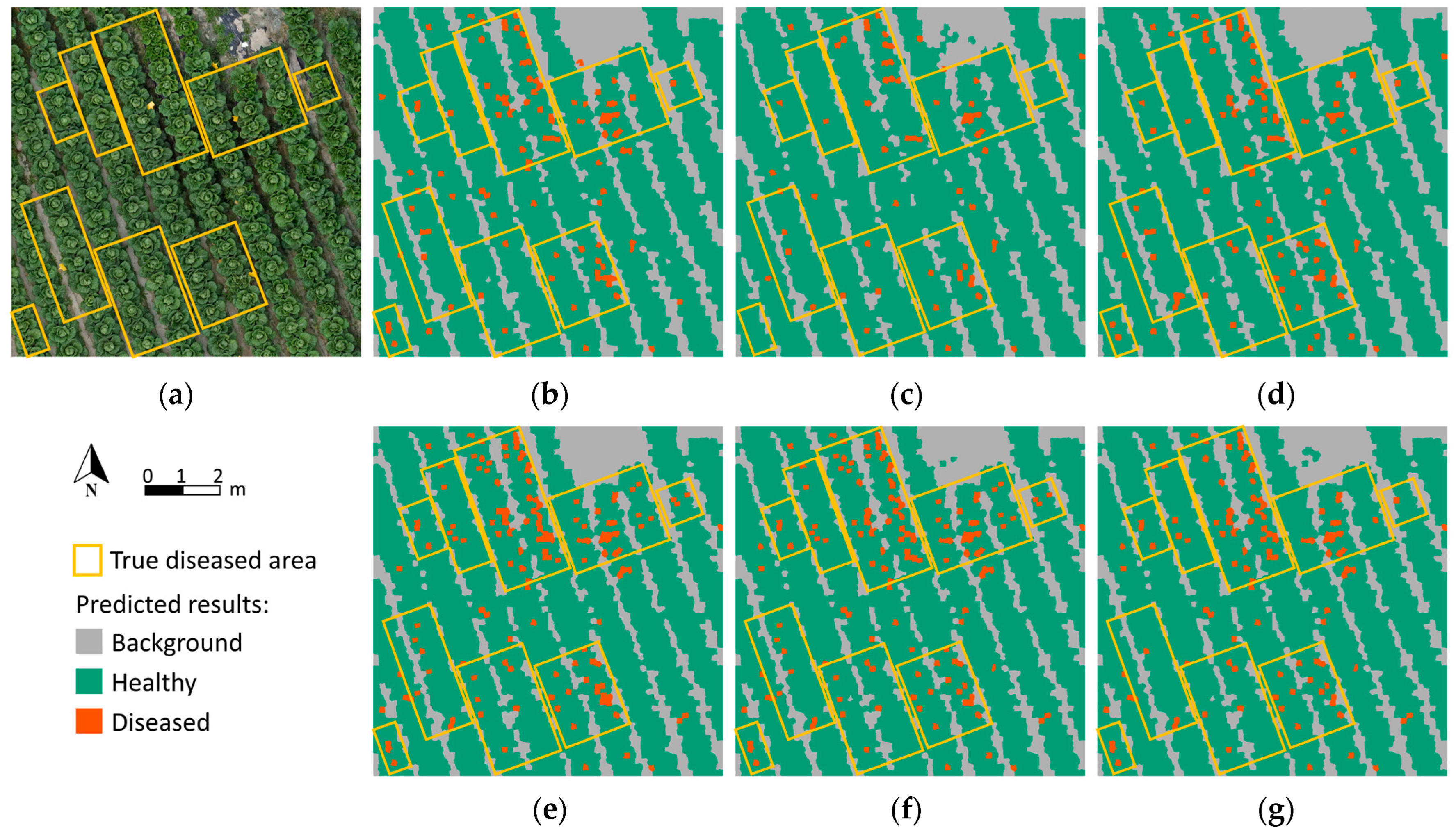
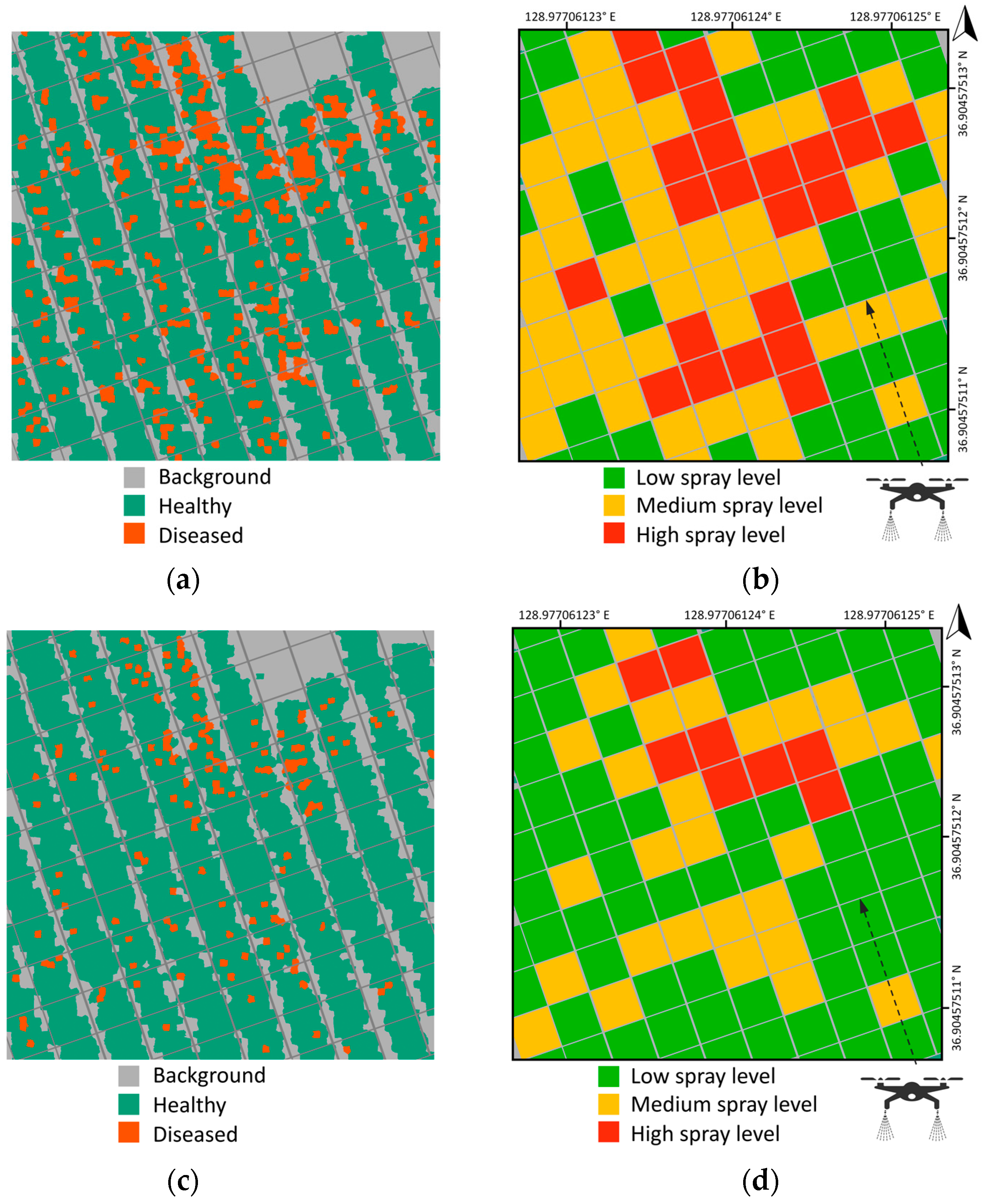
3.3. Classification Visualization and Prescription Map Generation

Figure 10 and Figure 11 present the classification visualization results of six models on the 25 October and 18 October test sets, respectively. Figure 10a displays the orthomosaic map of the 25 October test plot, where yellow boxes indicate ground-truth diseased areas, primarily consisting of cabbage leaves exhibiting mid-to-late-stage downy mildew symptoms. The classification outputs from each model (Figure 10b–g) visualize predicted background regions in gray, healthy leaves in green, and diseased leaves in orange. A strong spatial correspondence is evident between the predicted and actual diseased areas, confirming the model’s effectiveness in identifying mid-to-late-stage infections. Notably, MobileNetV3-Large (Figure 10d)—with a relatively low recall rate for diseased samples (0.826)—predicted fewer diseased regions than models such as TinyViT-5M (recall: 0.903; Figure 10f) and MobileViT-S (recall: 0.931; Figure 10g). Some predicted diseased areas outside the annotated ground-truth boxes may be attributable to misclassifications or, alternatively, instances where the model correctly identified mild symptoms that were overlooked during manual annotation. Figure 12 illustrates examples of such misclassifications, including diseased leaves labeled as healthy due to faint or inconspicuous lesions, and healthy leaves incorrectly classified as diseased due to yellowing or rough textures that visually resemble disease symptoms in RGB imagery.

In contrast, classification performance on the 18 October test set was lower, primarily due to the early to mid-stage nature of the disease during that period. At this stage, symptoms were less distinct in RGB images, thereby complicating visual differentiation. For instance, EfficientNet-B0 (Figure 11c)—with a diseased recall rate of 0.678—identified significantly fewer diseased regions than DeiT-Tiny (recall: 0.774; Figure 11e) and TinyViT-5M (recall: 0.757; Figure 11f). Additionally, environmental variations between image acquisition dates may have further impacted model performance. As illustrated in Figure 13, several diseased samples were misclassified as healthy due to subtle yellowish discoloration, while some healthy leaves were incorrectly classified as diseased because of bright leaf edges or yellow-tinted surfaces. Moreover, the training dataset was temporally biased toward samples collected on 25 October, causing the models to become more adept at identifying late-stage symptoms. Figure 14 illustrates the progression of the disease symptoms. On 18 October (Figure 14a,c), symptoms were mild, characterized by slight discoloration and subtle structural changes. By 25 October (Figure 14b,d), these symptoms had progressed to more visually prominent lesions and tissue damage. These findings highlight the need to improve early-stage disease detection by employing more balanced training datasets, applying contrastive learning techniques, and integrating multimodal data sources to increase sensitivity to subtle disease features and enhance detection accuracy.

Furthermore, variable-rate prescription maps were also developed to enable targeted pesticide application based on spatial disease severity. As shown in Figure 15a,c, classification outputs were divided into square zones aligned with crop rows and scaled to match the sprayer’s swath width. For each zone, the proportion of diseased pixels was computed and mapped to predefined severity levels (Figure 15b,d): low severity (<5%, green), indicating minimal or no pesticide application; medium severity (5–15%, yellow), indicating a need for medium-dose spraying; and high severity (>15%, red), indicating a need for high-dose application. Both the spatial resolution and zone dimensions can be adjusted to fit the capabilities of UAVs or ground-based sprayers. Similarly, severity thresholds and spray levels can be customized—for example, expanded to four or more categories—to match the control resolution of variable-rate sprayers. As the UAV imagery was georeferenced using GCPs, the prescription maps include high-precision geographic coordinates, enabling accurate integration with GPS-guided spraying systems for targeted and efficient disease management.

4. Discussion

This study proposed a UAV-based approach for detecting downy mildew in kimchi cabbage using RGB imagery and lightweight deep learning models. Six models—comprising both CNNs and ViT-based architectures—were evaluated to compare their classification performance and assess their suitability for deployment in edge computing and real-time field applications [36]. However, given the limited number and diversity of evaluated models, the observed performance differences should be interpreted within the scope of the selected architectures.

CNN-based models exhibited faster convergence speed and higher inference efficiency due to their hierarchical architectures and localized receptive fields. These architectural features make them particularly effective for detecting small, localized lesions typical of early disease stages. ResNet-18, employed as the baseline model, contains approximately 11.7 million parameters. Although not conventionally categorized as lightweight, its relatively shallow architecture and efficient convolutional blocks enabled fast training and inference speeds—surpassed only by MobileNetV3-Large, a model specifically optimized for mobile and real-time scenarios. However, the aggressive lightweighting of MobileNetV3-Large resulted in a trade-off in classification performance, ranking lowest among the six models in terms of detection accuracy [37]. In contrast, EfficientNet-B0, which employs a compound scaling method to balance network depth, width, and resolution, achieved higher accuracy than ResNet-18. Nonetheless, its increased computational demand led to longer training and inference times, and it showed weaker generalization performance across test dates [38].

Conversely, ViT-based models leverage global self-attention mechanisms, enabling more effective modeling of long-range dependencies and spatially distant contextual features [39]. This architectural strength made them more resilient to variations in lighting and imaging conditions across different acquisition dates. DeiT-Tiny, a representative lightweight ViT model, achieved competitive inference efficiency and demonstrated the highest cross-date generalization performance, highlighting the advantages of transformer-based global feature extraction. Hybrid models such as TinyViT-5M and MobileViT-S, which integrate CNN-based local feature extraction with transformer-based global attention, offered a balanced solution. These models effectively captured both fine-grained local details and broader contextual cues, resulting in strong classification accuracy and stable performance across acquisition dates. However, this hybrid design introduced additional architectural complexity, resulting in slightly longer training and inference times compared with their pure CNN or ViT counterparts. Despite these computational trade-offs, the hybrid models showed promising potential for further development, particularly in precision agriculture applications where both accuracy and adaptability are essential. Their performance underscores the growing relevance of hybrid architectures in computer vision and their value as a research direction for robust plant disease detection in real-world field conditions [40].

Compared with pixel-level segmentation methods, SLIC-based leaf segmentation more effectively preserves spatial structure while enhancing feature learning at a lower computational cost [41]. However, its reliance on color and spatial proximity can introduce boundary inaccuracies, particularly in cases of overlapping or densely clustered leaves [42]. Additionally, segmentation performance depends on hyperparameter tuning, which may require adjustments for different field conditions [43]. Although leaf-level segmentation improves classification accuracy, it does not directly translate to field-scale disease mapping, which is crucial for precision agriculture applications. Post-processing techniques, such as clustering or region-merging algorithms, could transform leaf-level predictions into spatially coherent disease density maps, enabling variable-rate pesticide application [44]. Future research should explore deep learning-based segmentation methods (e.g., U-Net and DeepLabV3+) or multi-scale segmentation strategies to improve segmentation precision and disease mapping accuracy [45].

Despite being conducted under real-world field conditions, this study encountered several dataset limitations that posed challenges in disease classification. The dataset exhibited significant class imbalance, with most diseased samples collected on 25 October, resulting in a training bias toward late-stage symptoms. Although data augmentation techniques were applied to mitigate this issue, early-stage recall remained low, highlighting the need for more balanced datasets. A major limitation of this study is its reliance on data collected from a single field over the span of one week. This narrow scope may fail to capture critical variations in environmental factors—such as lighting, humidity, and temperature—as well as differences in cabbage cultivars and disease progression patterns. These factors can influence symptom expression and cause domain shifts, thereby limiting the generalizability of the trained models [46]. Traditional augmentation techniques often fail to replicate real-world variations in disease appearance, as observed in symptom progression between 18 October and 25 October [47]. Cross-date evaluations confirmed that disease progression significantly impacted early-stage recall, which declined over time. Few-shot learning and contrastive learning have shown potential in improving model generalization under limited data conditions, making them promising approaches for future research [48]. Future research should consider expanding data collection across multiple fields, seasons, and cabbage cultivars, and exploring domain adaptation to improve robustness against variations in symptom expression and environmental conditions.

This study employed transfer learning by initializing deep learning models with ImageNet-pretrained weights for UAV-based cabbage disease detection. This approach reduced the need for extensive labeled datasets and improved training efficiency [49]. However, since most pretrained models are trained on general-purpose datasets (e.g., ImageNet), they may not fully capture the distinct visual characteristics of plant diseases, particularly during early infection stages [50]. Future research should explore pretrained models specifically tailored for plant disease classification to enhance feature extraction in agricultural imaging applications. Furthermore, because this study was conducted in a single experimental field, model generalization to different climates, soil types, and cabbage cultivars remains uncertain. Expanding data collection across diverse agricultural environments is crucial for improving model robustness and ensuring wider applicability [51].

The prescription map developed in this study plays a critical role in precision agriculture, serving as a decision-support tool for variable-rate pesticide application. By analyzing the spatial distribution of predicted diseased leaves from the classification results, the proposed framework facilitates the rapid generation of zoned management maps. These maps offer flexible configurability, including adjustable zone sizes and customizable spray intensity levels, and incorporate high-precision geolocation data derived from georeferenced UAV imagery. This adaptability enables seamless alignment with various spraying platforms—whether UAV-based or ground-based—by matching spray swath widths and control resolution. This spatially informed approach facilitates targeted pesticide application based on localized disease severity, thereby enhancing treatment precision and optimizing resource use. However, real-time decoding and operational deployment of prescription maps in large-scale field conditions remain significant technical challenges [52]. Ensuring timely and autonomous guidance for spraying platforms will require further advancements in prescription map usability and system integration, particularly regarding end-user interface design, platform responsiveness, and compatibility across diverse variable-rate spraying systems.

This study confirmed the feasibility of UAV-based RGB imaging for kimchi cabbage disease detection. RGB cameras effectively capture visual features, such as color, shape, and texture, enabling efficient identification of advanced disease symptoms [53]. However, the spectral limitations of RGB imaging hinder early-stage disease detection, as physiological changes during early stages of infection are not easily distinguishable within the visible wavelength range [54]. Kuswidiyanto et al. demonstrated that RE bands significantly improve early symptom detection, particularly for downy mildew [7]. Their study, which employed hyperspectral imaging combined with a 3D-ResNet model, achieved high recall for both early- and late-stage infections. While the current study focused on cost-effective RGB imaging, future research should explore RGB–RE fusion strategies to improve early-stage disease detection while maintaining the feasibility of UAV-based monitoring [55].

5. Conclusions

This study proposed an efficient UAV-based approach for detecting downy mildew in kimchi cabbage using RGB imaging and lightweight deep learning models. A tile-wise image processing strategy, coupled with SLIC-based leaf segmentation, enabled fine-scale disease classification from high-resolution UAV orthomosaics. Among the models evaluated, ViT-based architectures consistently outperformed traditional CNN-based models in terms of classification accuracy and generalization capability. For late-stage disease detection, DeiT-Tiny achieved the highest test accuracy (0.948) and macro F1-score (0.913), while MobileViT-S recorded the highest diseased recall (0.931). Conversely, for early-stage detection, TinyViT-5M achieved the highest test accuracy (0.970) and macro F1-score (0.918). However, diseased recall declined across all models under early-stage conditions, with DeiT-Tiny achieving the highest value at 0.774. These results underscore the inherent challenges of identifying early symptoms using RGB imagery alone. To support precision management, the classification results were further utilized to generate variable-rate prescription maps based on spatial disease severity. Zone size, severity thresholds, and the number of application levels can be flexibly adjusted to align with practical field requirements and equipment specifications. Overall, the findings demonstrate the feasibility of deploying lightweight models within UAV operational constraints and translating model predictions into actionable strategies for targeted disease control. Future research should explore the fusion of RGB and red-edge data, as well as the integration of multi-temporal imagery, to improve classification performance and enhance model robustness across varying disease stages and environmental conditions.

References

1. Niu, X.; Leung, H.; Williams, P.H. Sources and Nature of Resistance to Downy Mildew and Turnip Mosaic in Chinese Cabbage. J. Am. Soc. Hortic. Sci. 1983, 108, 775–778. [Google Scholar] [CrossRef]
2. Kouadio, L.; El Jarroudi, M.; Belabess, Z.; Laasli, S.-E.; Roni, M.Z.K.; Amine, I.D.I.; Mokhtari, N.; Mokrini, F.; Junk, J.; Lahlali, R. A Review on UAV-Based Applications for Plant Disease Detection and Monitoring. Remote Sens. 2023, 15, 4273. [Google Scholar] [CrossRef]
3. Barbedo, J. A Review on the Use of Unmanned Aerial Vehicles and Imaging Sensors for Monitoring and Assessing Plant Stresses. Drones 2019, 3, 40. [Google Scholar] [CrossRef]
4. Kuswidiyanto, L.W.; Noh, H.-H.; Han, X. Plant Disease Diagnosis Using Deep Learning Based on Aerial Hyperspectral Images: A Review. Remote Sens. 2022, 14, 6031. [Google Scholar] [CrossRef]
5. Adão, T.; Hruška, J.; Pádua, L.; Bessa, J.; Peres, E.; Morais, R.; Sousa, J. Hyperspectral Imaging: A Review on UAV-Based Sensors, Data Processing and Applications for Agriculture and Forestry. Remote Sens. 2017, 9, 1110. [Google Scholar] [CrossRef]
6. Zhang, N.; Yang, G.; Pan, Y.; Yang, X.; Chen, L.; Zhao, C. A Review of Advanced Technologies and Development for Hyperspectral-Based Plant Disease Detection in the Past Three Decades. Remote Sens. 2020, 12, 3188. [Google Scholar] [CrossRef]
7. Kuswidiyanto, L.W.; Wang, P.; Noh, H.H.; Jung, H.Y.; Jung, D.H.; Han, X. Airborne Hyperspectral Imaging for Early Diagnosis of Kimchi Cabbage Downy Mildew Using 3D-ResNet and Leaf Segmentation. Comput. Electron. Agric. 2023, 214, 108312. [Google Scholar] [CrossRef]
8. Datta, D.; Mallick, P.K.; Bhoi, A.K.; Ijaz, M.F.; Shafi, J.; Choi, J. Hyperspectral Image Classification: Potentials, Challenges, and Future Directions. Comput. Intell. Neurosci. 2022, 2022, 3854635. [Google Scholar] [CrossRef]
9. Bioucas-Dias, J.M.; Plaza, A.; Camps-Valls, G.; Scheunders, P.; Nasrabadi, N.; Chanussot, J. Hyperspectral Remote Sensing Data Analysis and Future Challenges. IEEE Geosci. Remote Sens. Mag. 2013, 1, 6–36. [Google Scholar] [CrossRef]
10. Neupane, K.; Baysal-Gurel, F. Automatic Identification and Monitoring of Plant Diseases Using Unmanned Aerial Vehicles: A Review. Remote Sens. 2021, 13, 3841. [Google Scholar] [CrossRef]
11. Guo, H.; Cheng, Y.; Liu, J.; Wang, Z. Low-Cost and Precise Traditional Chinese Medicinal Tree Pest and Disease Monitoring Using UAV RGB Image Only. Sci. Rep. 2024, 14, 25562. [Google Scholar] [CrossRef] [PubMed]
12. Yuan, W.; Wijewardane, N.K.; Jenkins, S.; Bai, G.; Ge, Y.; Graef, G.L. Early Prediction of Soybean Traits through Color and Texture Features of Canopy RGB Imagery. Sci. Rep. 2019, 9, 14089. [Google Scholar] [CrossRef]
13. Pfordt, A.; Paulus, S. A Review on Detection and Differentiation of Maize Diseases and Pests by Imaging Sensors. J. Plant Dis. Prot. 2025, 132, 40. [Google Scholar] [CrossRef]
14. Shahi, T.B.; Xu, C.-Y.; Neupane, A.; Guo, W. Recent Advances in Crop Disease Detection Using UAV and Deep Learning Techniques. Remote Sens. 2023, 15, 2450. [Google Scholar] [CrossRef]
15. Abade, A.; Ferreira, P.A.; de Barros Vidal, F. Plant Diseases Recognition on Images Using Convolutional Neural Networks: A Systematic Review. Comput. Electron. Agric. 2021, 185, 106125. [Google Scholar] [CrossRef]
16. Tugrul, B.; Elfatimi, E.; Eryigit, R. Convolutional Neural Networks in Detection of Plant Leaf Diseases: A Review. Agriculture 2022, 12, 1192. [Google Scholar] [CrossRef]
17. Lu, J.; Tan, L.; Jiang, H. Review on Convolutional Neural Network (CNN) Applied to Plant Leaf Disease Classification. Agriculture 2021, 11, 707. [Google Scholar] [CrossRef]
18. Bhatt, D.; Patel, C.; Talsania, H.; Patel, J.; Vaghela, R.; Pandya, S.; Modi, K.; Ghayvat, H. CNN Variants for Computer Vision: History, Architecture, Application, Challenges and Future Scope. Electronics 2021, 10, 2470. [Google Scholar] [CrossRef]
19. Dosovitskiy, A.; Beyer, L.; Kolesnikov, A.; Weissenborn, D.; Zhai, X.; Unterthiner, T.; Dehghani, M.; Minderer, M.; Heigold, G.; Gelly, S.; et al. An Image Is Worth 16x16 Words: Transformers for Image Recognition at Scale. arXiv 2020, arXiv:2010.11929. [Google Scholar] [CrossRef]
20. Mehta, S.; Rastegari, M. MobileViT: Light-Weight, General-Purpose, and Mobile-Friendly Vision Transformer. arXiv 2022, arXiv:2110.02178. [Google Scholar] [CrossRef]
21. Wu, K.; Zhang, J.; Peng, H.; Liu, M.; Xiao, B.; Fu, J.; Yuan, L. Tinyvit: Fast pretraining distillation for small vision transformers. In Proceedings of the European Conference on Computer Vision, Tel Aviv, Israel, 23–27 October 2022; pp. 68–85. [Google Scholar] [CrossRef]
22. Singh, V.; Misra, A.K. Detection of Plant Leaf Diseases Using Image Segmentation and Soft Computing Techniques. Inf. Process. Agric. 2017, 4, 41–49. [Google Scholar] [CrossRef]
23. Nethala, P.; Um, D.; Vemula, N.; Montero, O.F.; Lee, K.; Bhandari, M. Techniques for Canopy to Organ Level Plant Feature Extraction via Remote and Proximal Sensing: A Survey and Experiments. Remote Sens. 2024, 16, 4370. [Google Scholar] [CrossRef]
24. Achanta, R.; Shaji, A.; Smith, K.; Lucchi, A.; Fua, P.; Süsstrunk, S. SLIC Superpixels Compared to State-of-the-Art Superpixel Methods. IEEE Trans. Pattern Anal. Mach. Intell. 2012, 34, 2274–2282. [Google Scholar] [CrossRef] [PubMed]
25. Choi, K.-S.; Oh, K.-W. Subsampling-Based Acceleration of Simple Linear Iterative Clustering for Superpixel Segmentation. Comput. Vis. Image Underst. 2016, 146, 1–8. [Google Scholar] [CrossRef]
26. Tetila, E.C.; Machado, B.B.; Menezes, G.K.; Da Silva Oliveira, A.; Alvarez, M.; Amorim, W.P.; De Souza Belete, N.A.; Da Silva, G.G.; Pistori, H. Automatic Recognition of Soybean Leaf Diseases Using UAV Images and Deep Convolutional Neural Networks. IEEE Geosci. Remote Sens. Lett. 2020, 17, 903–907. [Google Scholar] [CrossRef]
27. Karasiak, N.; Dejoux, J.-F.; Monteil, C.; Sheeren, D. Spatial Dependence between Training and Test Sets: Another Pitfall of Classification Accuracy Assessment in Remote Sensing. Mach. Learn. 2022, 111, 2715–2740. [Google Scholar] [CrossRef]
28. He, H.; Garcia, E.A. Learning from Imbalanced Data. IEEE Trans. Knowl. Data Eng. 2009, 21, 1263–1284. [Google Scholar] [CrossRef]
29. Buda, M.; Maki, A.; Mazurowski, M.A. A Systematic Study of the Class Imbalance Problem in Convolutional Neural Networks. Neural Netw. 2018, 106, 249–259. [Google Scholar] [CrossRef]
30. Enkvetchakul, P.; Surinta, O. Effective Data Augmentation and Training Techniques for Improving Deep Learning in Plant Leaf Disease Recognition. Appl. Sci. Eng. Prog. 2021, 15, 3810. [Google Scholar] [CrossRef]
31. Owusu-Adjei, M.; Ben Hayfron-Acquah, J.; Frimpong, T.; Abdul-Salaam, G. Imbalanced Class Distribution and Performance Evaluation Metrics: A Systematic Review of Prediction Accuracy for Determining Model Performance in Healthcare Systems. PLoS Digit. Health 2023, 2, e0000290. [Google Scholar] [CrossRef]
32. He, K.; Zhang, X.; Ren, S.; Sun, J. Deep Residual Learning for Image Recognition. In Proceedings of the Conference on Computer Vision and Pattern Recognition, Las Vegas, NV, USA, 30 June 2016. [Google Scholar]
33. Tan, M.; Le, Q.V. EfficientNet: Rethinking Model Scaling for Convolutional Neural Networks. In Proceedings of the International Conference on Machine Learning (ICML), Long Beach, CA, USA, 9–15 June 2019. [Google Scholar]
34. Howard, A.; Pang, R.; Adam, H.; Le, Q.; Sandler, M.; Chen, B.; Wang, W.; Chen, L.C.; Tan, M.; Chu, G.; et al. Searching for MobileNetV3. In Proceedings of the IEEE/CVF International Conference on Computer Vision, Seoul, Republic of Korea, 27 October–2 November 2019; pp. 1314–1324. [Google Scholar]
35. Touvron, H.; Cord, M.; Douze, M.; Massa, F.; Sablayrolles, A.; Jegou, H. Training data-efficient image transformers & distillation through attention. arXiv 2020, arXiv:2012.12877. [Google Scholar]
36. Wang, C.-H.; Huang, K.-Y.; Yao, Y.; Chen, J.-C.; Shuai, H.-H.; Cheng, W.-H. Lightweight Deep Learning: An Overview. IEEE Consum. Electron. Mag. 2024, 13, 51–64. [Google Scholar] [CrossRef]
37. Qian, S.; Ning, C.; Hu, Y. MobileNetV3 for Image Classification. In Proceedings of the 2021 IEEE 2nd International Conference on Big Data, Artificial Intelligence and Internet of Things Engineering (ICBAIE), Nanchang, China, 26–28 March 2021; pp. 490–497. [Google Scholar]
38. Hoang, V.-T.; Jo, K.-H. Practical Analysis on Architecture of EfficientNet. In Proceedings of the 2021 14th International Conference on Human System Interaction (HSI), Gdańsk, Poland, 8–10 July 2021; pp. 1–4. [Google Scholar]
39. Borhani, Y.; Khoramdel, J.; Najafi, E. A Deep Learning Based Approach for Automated Plant Disease Classification Using Vision Transformer. Sci. Rep. 2022, 12, 11554. [Google Scholar] [CrossRef] [PubMed]
40. Thakur, P.S.; Chaturvedi, S.; Khanna, P.; Sheorey, T.; Ojha, A. Vision Transformer Meets Convolutional Neural Network for Plant Disease Classification. Ecol. Inform. 2023, 77, 102245. [Google Scholar] [CrossRef]
41. Wu, X.; Liu, Y.; Xing, M.; Yang, C.; Hong, S. Image Segmentation for Pest Detection of Crop Leaves by Improvement of Regional Convolutional Neural Network. Sci. Rep. 2024, 14, 24160. [Google Scholar] [CrossRef]
42. Lin, X.; Li, C.-T.; Adams, S.; Kouzani, A.Z.; Jiang, R.; He, L.; Hu, Y.; Vernon, M.; Doeven, E.; Webb, L.; et al. Self-Supervised Leaf Segmentation under Complex Lighting Conditions. Pattern Recognit. 2023, 135, 109021. [Google Scholar] [CrossRef]
43. Javidan, S.M.; Banakar, A.; Rahnama, K.; Vakilian, K.A.; Ampatzidis, Y. Feature Engineering to Identify Plant Diseases Using Image Processing and Artificial Intelligence: A Comprehensive Review. Smart Agric. Technol. 2024, 8, 100480. [Google Scholar] [CrossRef]
44. Chen, L.C.; Zhu, Y.; Papandreou, G.; Schroff, F.; Adam, H. Encoder-decoder with atrous separable convolution for semantic image segmentation. In Proceedings of the European Conference on Computer Vision (ECCV), Munich, Germany, 8–14 September 2018; pp. 801–818. [Google Scholar]
45. Wang, C.; Du, P.; Wu, H.; Li, J.; Zhao, C.; Zhu, H. A Cucumber Leaf Disease Severity Classification Method Based on the Fusion of DeepLabV3+ and U-Net. Comput. Electron. Agric. 2021, 189, 106373. [Google Scholar] [CrossRef]
46. Mohanty, S.P.; Hughes, D.P.; Salathé, M. Using Deep Learning for Image-Based Plant Disease Detection. Front. Plant Sci. 2016, 7, 1419. [Google Scholar] [CrossRef]
47. Lu, Y.; Chen, D.; Olaniyi, E.; Huang, Y. Generative Adversarial Networks (GANs) for Image Augmentation in Agriculture: A Systematic Review. Comput. Electron. Agric. 2022, 200, 107208. [Google Scholar] [CrossRef]
48. Wang, Y.; Yao, Q.; Kwok, J.T.; Ni, L.M. Generalizing from a Few Examples. ACM Comput. Surv. 2021, 53, 63. [Google Scholar] [CrossRef]
49. Shin, H.-C.; Roth, H.R.; Gao, M.; Lu, L.; Xu, Z.; Nogues, I.; Yao, J.; Mollura, D.; Summers, R.M. Deep Convolutional Neural Networks for Computer-Aided Detection: CNN Architectures, Dataset Characteristics and Transfer Learning. IEEE Trans. Med. Imaging 2016, 35, 1285–1298. [Google Scholar] [CrossRef] [PubMed]
50. Al Sahili, Z.; Awad, M. The Power of Transfer Learning in Agricultural Applications: AgriNet. Front. Plant Sci. 2022, 13, 992700. [Google Scholar] [CrossRef] [PubMed]
51. Weersink, A.; Fraser, E.; Pannell, D.; Duncan, E.; Rotz, S. Opportunities and Challenges for Big Data in Agricultural and Environmental Analysis. Annu. Rev. Resour. Econ. 2018, 10, 19–37. [Google Scholar] [CrossRef]
52. Luo, S.; Wen, S.; Zhang, L.; Lan, Y.; Chen, X. Extraction of crop canopy features and decision-making for variable spraying based on unmanned aerial vehicle LiDAR data. Comput. Electron. Agric. 2024, 224, 109197. [Google Scholar] [CrossRef]
53. Ahmad, N.; Asif, H.M.S.; Saleem, G.; Younus, M.U.; Anwar, S.; Anjum, M.R. Leaf Image-Based Plant Disease Identification Using Color and Texture Features. Wirel. Pers. Commun. 2021, 121, 1139–1168. [Google Scholar] [CrossRef]
54. Ban, S.; Tian, M.; Hu, D.; Xu, M.; Yuan, T.; Zheng, X.; Li, L.; Wei, S. Evaluation and Early Detection of Downy Mildew of Lettuce Using Hyperspectral Imagery. Agriculture 2025, 15, 444. [Google Scholar] [CrossRef]
55. Ahmad, U.; Nasirahmadi, A.; Hensel, O.; Marino, S. Technology and Data Fusion Methods to Enhance Site-Specific Crop Monitoring. Agronomy 2022, 12, 555. [Google Scholar] [CrossRef]
Figure 1. Schematic comparison of image classification architectures: (a) Convolutional Neural Network (CNN), which extracts local hierarchical features using convolutional layers, and (b) Vision Transformer (ViT), which models global contextual relationships through patch embeddings and self-attention mechanisms. L× represents repeated encoder blocks, each comprising a multi-head self-attention mechanism and a multi-layer perceptron (MLP).
Remotesensing 17 02388 g001
Figure 2. Overview of the study workflow, from unmanned aerial vehicle (UAV)-based data acquisition to image processing, model training, and performance evaluation.
Remotesensing 17 02388 g002
Figure 3. Study area delineation. The white box outlines the kimchi cabbage field, with designated training plots (blue), validation plots (green), and test plots (yellow) for model development and evaluation.
Remotesensing 17 02388 g003
Figure 4. UAV-based data acquisition and field survey: (a) UAV and camera setup for aerial imaging, and (b) field survey with cabbages marked for downy mildew symptom assessment.
Remotesensing 17 02388 g004
Figure 5. Simple Linear Iterative Clustering (SLIC)-based image segmentation and disease sample labeling using an interactive annotation interface.
Remotesensing 17 02388 g005
Figure 6. Examples of labeled samples: (a) Background, (b) healthy cabbage leaves, and (c) diseased cabbage leaves.
Remotesensing 17 02388 g006
Figure 7. Training and validation accuracy curves for each deep learning model evaluated in this study: (a) ResNet-18, (b) EfficientNet-B0, (c) MobileNetV3-Large, (d) DeiT-Tiny, (e) TinyViT-5M, and (f) MobileViT-S.
Remotesensing 17 02388 g007aRemotesensing 17 02388 g007b
Figure 8. Normalized confusion matrices comparing model predictions on the 25 October test set: (a) ResNet-18, (b) EfficientNet-B0, (c) MobileNetV3-Large, (d) DeiT-Tiny, (e) TinyViT-5M, and (f) MobileViT-S.
Remotesensing 17 02388 g008
Figure 9. Normalized confusion matrices illustrating the classification performance of each model on the 18 October test set: (a) ResNet-18, (b) EfficientNet-B0, (c) MobileNetV3-Large, (d) DeiT-Tiny, (e) TinyViT-5M, and (f) MobileViT-S.
Remotesensing 17 02388 g009
Figure 10. Orthomosaic and classification results for the 25 October test set: (a) orthomosaic of the test plot; classification outputs from (b) ResNet-18, (c) EfficientNet-B0, (d) MobileNetV3-Large, (e) DeiT-Tiny, (f) TinyViT-5M, and (g) MobileViT-S. In the classification maps, background areas are shown in gray, healthy cabbage leaves in green, and diseased leaves in orange. Yellow boxes indicate ground-truth diseased regions, primarily corresponding to mid-to-late-stage downy mildew symptoms.
Remotesensing 17 02388 g010
Figure 11. Orthomosaic and classification results for the 18 October test set: (a) orthomosaic of the test plot; classification outputs from (b) ResNet-18, (c) EfficientNet-B0, (d) MobileNetV3-Large, (e) DeiT-Tiny, (f) TinyViT-5M, and (g) MobileViT-S. In the classification maps, background regions are shown in gray, healthy cabbage leaves in green, and diseased leaves in orange. Yellow boxes represent ground-truth diseased areas, primarily corresponding to early-stage downy mildew symptoms.
Remotesensing 17 02388 g011
Figure 12. Examples of misclassified samples in the 25 October test set: (a) Diseased samples incorrectly classified as healthy, and (b) healthy samples incorrectly classified as diseased.
Remotesensing 17 02388 g012
Figure 13. Examples of misclassified samples in the 18 October test set: (a) diseased samples incorrectly classified as healthy, and (b) healthy samples incorrectly classified as diseased.
Remotesensing 17 02388 g013
Figure 14. Progression of downy mildew symptoms from early to mid-to-late stages between 18 October and 25 October: (a) field-level symptoms observed on 18 October (early stage), (b) field-level symptoms observed on 25 October (mid-to-late stage), (c) representative diseased leaf samples collected on 18 October (early stage), and (d) representative diseased leaf samples collected on 25 October (mid-to-late stage).
Remotesensing 17 02388 g014
Figure 15. Prescription maps generated based on classification results from the TinyViT-5M model: (a,b) classification and corresponding prescription maps for the 25 October test set; (c,d) classification and corresponding prescription maps for the 18 October test set. The classification maps were segmented into square zones aligned with crop rows and scaled to match the sprayer’s swath width. Disease severity within each zone was quantified based on the proportion of pixels predicted as diseased and categorized into three spray levels: low (<5%, green), medium (5–15%, yellow), and high (>15%, red). The threshold values and zone dimensions can be adjusted to suit practical field requirements.
Remotesensing 17 02388 g015