Dual-Branch Spatial–Spectral Transformer with Similarity Propagation for Hyperspectral Image Classification

Abstract

In recent years, Vision Transformers (ViTs) have gained significant traction in the field of hyperspectral image classification due to their advantages in modeling long-range dependency relationships between spectral bands and spatial pixels. However, after stacking multiple Transformer encoders, challenges pertaining to information degradation may emerge during the forward propagation. That is to say, existing Transformer-based methods exhibit certain limitations in retaining and effectively utilizing information throughout their forward transmission. To tackle these challenges, this paper proposes a novel dual-branch spatial–spectral Transformer model that incorporates similarity propagation (DBSSFormer-SP). Specifically, this model first employs a Hybrid Pooling Spatial Channel Attention (HPSCA) module to integrate global information by pooling across different dimensional directions, thereby enhancing its ability to extract salient features. Secondly, we introduce a mechanism for transferring similarity attention that aims to retain and strengthen key semantic features, thus mitigating issues associated with information degradation. Additionally, the Spectral Transformer (SpecFormer) module is employed to capture long-range dependencies among spectral bands. Finally, the extracted spatial and spectral features are fed into a multilayer perceptron (MLP) module for classification. The proposed method is evaluated against several mainstream approaches on four public datasets. Experimental results demonstrate that DBSSFormer-SP exhibits excellent classification performance.

1. Introduction

Hyperspectral imaging (HSI) plays a crucial role in various applications within the field of remote sensing. HSI encompasses tens to hundreds of narrow, continuous spectral bands that span from the visible spectrum to near-infrared wavelengths. Consequently, HSI provides rich information regarding ground features. It is instrumental in agricultural technology [1], resource exploration [2], urban planning [3] and military applications [4]. To fully harness the potential of HSI, researchers have developed numerous methodologies including unmixing [5], sharpening [6], super-resolution [7] and classification [8]. Among these, hyperspectral image classification (HSIC) stands out as one of the key areas of research within HSI. The HSIC process involves assigning specific labels to individual pixel units. Initially, researchers proposed a variety of classical methods primarily focused on feature extraction techniques and traditional machine learning approaches. Classical feature extraction methods encompass Principal Component Analysis (PCA) [9] and linear discriminant analysis (LDA) [10], among others. These techniques facilitate feature selection and dimensionality reduction on the input hyperspectral data, enabling the extraction of discriminative spectral features. Furthermore, traditional machine learning algorithms are employed for classification purposes, including Support Vector Machines (SVMs) [11], Random Forest (RF) algorithms [12], and K-Nearest Neighbor (KNN) algorithms [13]. However, many conventional methods fail to effectively leverage spatial information, which can adversely affect classification accuracy.

In recent years, researchers have increasingly focused on the field of deep learning due to its ability to automatically learn abstract features from raw data. This shift has led to remarkable advancements in the domain of computer vision. Currently, deep learning exhibits exceptional performance in HSIC, with many HSIC accuracies achieved through deep learning models surpassing those of traditional methods. Chen et al. [14] previously employed a stacking approach using varying numbers of autoencoders to extract different levels of spatial–spectral features. However, compressing input features into one-dimensional vectors results in a partial loss of spatial information. Subsequently, Convolutional Neural Networks (CNNs) have emerged as a significant advancement within deep learning. Due to their advantages such as weight sharing and local connectivity, along with their capability to extract extensive spatial and spectral features from hyperspectral images, CNNs have become prominent methodologies in this field. Hu et al. [15] designed a Convolutional Neural Network comprising five layers specifically for processing spectral information. To enhance the extraction of spatial information from HSI images, Zhao et al. [16] proposed utilizing 2D-CNNs for extracting spatial features and integrating them with spectral features obtained through local discriminative embedding methods, thereby improving classification accuracy. Yue et al. [17] proposed the use of 2D-CNN to extract spatial spectral features, employing logistic regression for classification. Yang et al. [18] implemented a dual-branch CNN architecture that utilized both 1D-CNN and 2D-CNN to separately extract spectral and spatial features, respectively. The two feature sets were then concatenated and forwarded to a fully connected layer, resulting in improved classification accuracy. However, the limitation of this approach is that 1D-CNN focuses solely on the spectral vector while 2D-CNN addresses only the spatial vector; thus, effective integration of these two types of features remains challenging. To address this issue, Chen et al. [19] introduced a 3D-CNN model designed for the enhanced extraction of spatial–spectral features and experimentally demonstrated its superior classification accuracy compared to previous methods. Roy et al. [20] employed a hybrid CNN structure that first utilized 3D-CNN to capture spectral–spatial features before applying 2D-CNN for further extraction of spatial characteristics. This methodology not only facilitates the learning of more advanced feature representations but also significantly reduces the computational burden on the model. Zhou et al. [21] proposed the Spatial–Spectral Pyramid Network (SSPN) model for HSIC, which innovatively combined a 3D Convolutional Neural Network with feature pyramids while introducing multi-scale convolution kernels to extract local features across varying receptive fields. This approach achieves multilevel feature fusion and markedly enhances feature expressiveness. Deep Convolutional Neural Networks (CNNs) are capable of capturing more global feature representations by incrementally stacking multiple convolutional layers, thereby improving classification accuracy. However, this advancement introduces new challenges; specifically, an increase in network depth can exacerbate issues related to gradient vanishing or explosion, ultimately leading to diminished classification performance. Zhong et al. [22] introduced the residual network architecture to enhance effective information transmission within neural networks. This connection method aids in preserving original feature information, partially alleviating the gradient vanishing problem, and ultimately improving classification performance. Zhu et al. [23] proposed the Residual Spectral–Spatial Attention Network (RSSAN), which incorporates an attention mechanism to strengthen spatial–spectral features while employing Convolutional Neural Networks (CNNs) and residual blocks to jointly refine features across multiple levels. Cui et al. [24] decomposed standard 3D convolution into depthwise convolution and pointwise convolution, achieving a lightweight design that significantly reduces parameters while maintaining high classification accuracy.

Beyond the aforementioned CNN-based approaches, a variety of networks exhibiting exceptional performance have been utilized in the context of HSIC. Mou et al. [25] introduced an RNN framework for HSIC that employs Parametric Rectified Tanh (PRetanh) and a Gated Recurrent Unit (GRU) to analyze hyperspectral sequences, thereby facilitating efficient feature learning. Paoletti et al. [26] enhanced the CNN architecture by incorporating a spectral space capsule network. This capsule network not only learns spectral–spatial features but also considers spatial locations and their associated spectral characteristics. In addition to these advancements, there are various network architectures based on Generative Adversarial Networks (GANs) [27,28], Graph Convolutional Networks (GCNs) [29,30], and other models that demonstrate strong classification performance.

The network architecture based on Convolutional Neural Networks (CNNs) has exhibited exceptional performance in extracting local features. However, the receptive field of CNNs is constrained by both the size of the convolutional kernel and the number of stacked layers. This limitation also restricts a CNN’s ability to capture long-range contextual information. In 2017, a team at Google introduced a novel model architecture known as Transformer. Unlike CNNs, Transformers leverage a self-attention mechanism (SA) to compute the degree of correlation between elements within the model, thereby effectively capturing long-range dependencies. The introduction of ViT [31] signifies that Transformers have been successfully applied to computer vision tasks. Following this development, ViT and its variants have found applications in hyperspectral image classification. From the perspective of spectral sequence information, Hong et al. [32] proposed a structure called SpectralFormer (SF), which utilizes Transformers to learn local spectral sequence information from adjacent spectral bands in hyperspectral images. They also incorporated skip connections to enhance information transitivity. He et al. [33] introduced the Spatial–Spectral Transformer (SST), which integrates both the CNN and Transformer architectures. In this approach, CNNs are employed to capture spatial features, while densely connected Transformer designs are utilized for feature extraction as well. This dual strategy not only facilitates rich feature extraction but also helps mitigate issues related to gradient vanishing. Finally, a multilayer perceptron (MLP) was employed for classification purposes. Sun et al. [34] proposed a novel classification method known as SSFTT, which transforms spatial and spectral features using a Gaussian distribution-weighted tokenizer and employs a Transformer to model these features, thereby enhancing the extraction of semantic information. However, SSFTT may suffer from inaccuracies in feature labeling. To address this issue, Zou et al. [35] introduced LESSFormer, which first generates representative spatial–spectral labels through a feature labeling module before utilizing a Transformer to improve feature expression capabilities. Mei et al. [36] contend that the features extracted via the multi-head self-attention mechanism (MHSA) tend to be overly discrete; thus, they proposed the Group-Aware Hierarchical Transformer (GAHT) model. By incorporating the Grouped Pixel Embedding (GPE) module, discriminative features are extracted from non-overlapping channels. This is then integrated with a Transformer architecture where attention is confined to local spatial–spectral contexts to mitigate issues related to feature dispersion. Yang et al. [37] proposed a novel Transformer network, QTN, which introduces BASM to dynamically select appropriate spectral bands. Additionally, it employs quaternion attention to capture local features and global long-range dependencies. The model has demonstrated excellent classification performance across multiple datasets. Roy et al. [38] introduced a novel classification model named MorphFormer, which integrates mathematical morphological operations to enhance the traditional attention mechanism. This model effectively extracts both morphological spatial and spectral features while improving the interaction of structural shape information among different tokens through morphological convolution. Zhao et al. [39] proposed a Transformer architecture known as the Group Separable Convolutional Transformer (GSC-ViT). This model captures local spatial–spectral features via a group separable convolution module and subsequently extracts local–global spatial features using a group separable self-attention mechanism (GSSA). The GSC-ViT demonstrates commendable classification accuracy while maintaining a lightweight design.

However, CNNs and Transformers tend to focus on singular aspects of representation. To address this limitation, Yang et al. [40] proposed an excellent classification model known as the Adaptive Coupling Transformer Network (ACTN). This model effectively extracts both local and global information, adaptively fusing the two to enhance the expressive power of features.

Although existing deep learning-based methods achieve commendable performance in HSIC, we have observed that certain Transformer-based approaches incorporate multiple Transformer encoders. This necessitates the repeated transmission of spatial–spectral information, which may result in the loss or degradation of some data. Some Transformer-based methods address this issue by integrating residual networks between adjacent Transformers and fusing feature information across layers. The features captured by deep networks are typically high-level and abstract, while shallow networks tend to capture low-level, more interpretable features. There exists a gap between these two distinct levels of features, and merely employing residual connections is insufficient for effective fusion. Sun et al. [41] recognized this challenge and proposed a novel method called MASSFormer method. They utilized convolutional layers to extract shallow spectral–spatial features, subsequently applying pooling to convert these features into memory tokens that are then expanded into each Transformer encoder. This approach effectively preserves the original feature information for subsequent Transformers, thereby mitigating the impact of information degradation to some extent. However, it is important to note that the shallow features employed by each Transformer encoder in MASSFormer remain consistent across all encoders, resulting in a lack of cross-layer interaction among them. Consequently, the noise present in the shallow features may be redundantly exploited and continuously propagated throughout the training process, ultimately affecting classification performance.

Furthermore, the recently emerged Mamba has made significant progress in modeling long sequence dependencies and has demonstrated potential in HSIC tasks. Chen et al. [42] proposed the RSMamba structure, which enhances the modeling capability for non-causal data through a multi-path activation mechanism, achieving commendable classification results across multiple datasets. However, the design of the Mamba structure primarily targets general sequence tasks and lacks adaptation for joint modeling of spatial–spectral features in hyperspectral imaging (HSI). Additionally, the Mamba network relies on a recursive state update mechanism that limits its ability to preserve local spatial details. This may result in shallow local discriminative information being weakened within deeper features, ultimately affecting the model’s classification performance.

To more effectively address the issues of information loss and underutilization resulting from the stacking of multiple Transformer encoders, this paper proposes a Dual-Branch Spatial–Spectral Transformer with Similarity Propagation (DBSSFormer-SP). The model comprises two branches that independently extract spatial and spectral features.

Despite the increasing prevalence of Transformer-based dual-branch architectures in hyperspectral image classification [43], these methods generally face two critical issues: on one hand, the spatial branch overlooks the degradation of feature extraction capabilities caused by stacking Transformer blocks; on the other hand, the spectral branch fails to adequately model the global correlations among various spectral bands.

In this paper, we propose DBSSFormer-SP, which introduces attention propagation to facilitate attention guidance from shallow to deep layers, effectively alleviating issues related to deep feature degradation and information ambiguity. Additionally, by employing a spectral Transformer module that models global dependencies between bands and integrating convolutional operations, our approach successfully extracts discriminative spectral features.

In detail, within the spatial branch, shallow spatial–spectral features are initially extracted through shallow convolutional layers. Subsequently, to fully leverage the spatial information present in hyperspectral images, we employ a Hybrid Pooling Spatial Channel Attention (HPSCA) module designed to enhance the discriminative capability of these features. The tokens generated from the flattened features serve as input for the Transformer encoders. We introduce a transitive similarity mechanism across adjacent Transformer encoders, which facilitates the transfer of low-level attention distributions to higher-level encoders via nonlinear transformations. This approach not only enhances information circulation but also ensures effective fusion of attention distributions across different levels. In the spectral branch, we utilize Transformers to capture dependencies among non-local bands within one-dimensional spectral sequences. Ultimately, both feature sets are integrated into a linear classifier for pixel label determination.

The three primary contributions of this paper are as follows:

(1)

DBSSFormer-SP is proposed, in which, to enhance the expressive capability of spatial features, we design a Hybrid Pooling Spatial Channel Attention (HPSCA) module. This module captures various long-range dependencies through attention mechanisms across different dimensions and integrates spatial information into the channel attention map to acquire global information dependencies. Subsequently, the channel dimension is compressed to generate spatial attention weights, thereby augmenting the discriminative power of spatial features.

(2)

This paper introduces a Similarity Propagation Transformer Encoder (SPTE) module. This module effectively integrates information by transferring the attention distribution across different encoder layers and employing nonlinear transformations. The transmission of information is enhanced, facilitating the interaction among various characteristic features. While it strengthens the representation of salient features, it also mitigates the issue of information attenuation commonly encountered in deep networks, thereby improving the classification performance of the model.

(3)

To effectively capture the relationships among spectral features, we propose the Spectral Transformer (SpecFormer) module. This module replaces the multilayer perceptron found in traditional Transformers with depth-wise separable convolutions. This approach not only enhances the ability to discern relationships between different spectral bands and emphasizes key spectral features but also significantly reduces both the number of parameters and their computational complexity.

The remainder of this paper is organized as follows: Section 2 details the implementation of the proposed method. Section 3 provides an overview of the dataset, outlines the design of experimental parameters, and presents the experimental results. Section 4 discusses the conclusions drawn from these experiments. Finally, Section 5 summarizes the key findings of this study and suggests directions for future research improvements.

2. Methodology

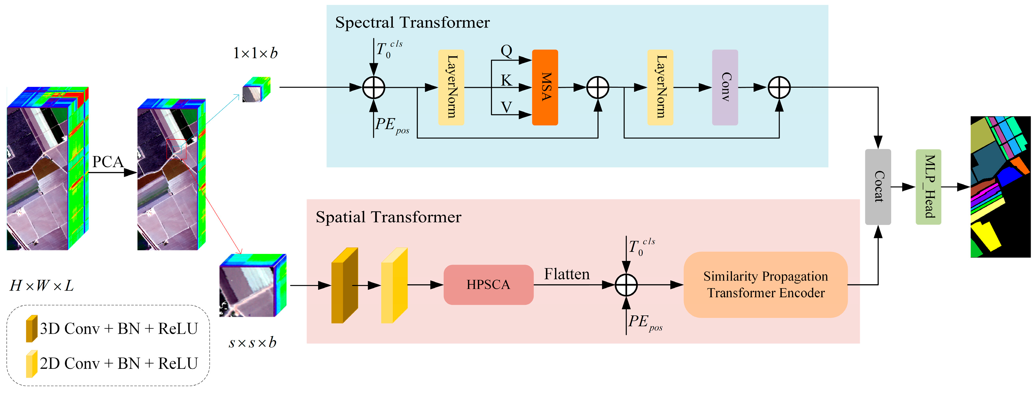
The overall structure of the proposed approach is presented in Figure 1. It primarily consists of hyperspectral data preprocessing, a Hybrid Pooling Spatial Channel Attention (HPSCA) module, and a Similarity Propagation Transformer Encoder (SPTE) for the spatial branch. Additionally, it includes the spectral branch of the Spectral Transformer (SpecFormer) module.

2.1. Hyperspectral Data Preprocessing

Hyperspectral data typically encompass hundreds of spectral bands, which provides extensive spectral information but also introduces a significant amount of redundant data. We employed Principal Component Analysis (PCA) to reduce the dimensionality of the original hyperspectral data, thereby compressing the spectral bands. PCA identifies orthogonal principal component directions that maximize variance across all samples, effectively eliminating redundant information while preserving essential details, thus reducing computational complexity. The HSI data cube is represented as $X\in {ℝ}^{H\times W\times L}$, where $H$, $W$, and $L$ denote the height, width, and number of spectral bands in the HSI dataset, respectively. PCA facilitates the reduction in the number of bands from $L$ to $b$, while maintaining the overall size of the HSI space. Consequently, after applying PCA for dimensionality reduction, the transformed HSI data can be expressed as $X\in {ℝ}^{H\times W\times b}$. Where $b$ signifies the number of spectral bands post-dimension reduction.

Subsequently, we extract the 3D block $X_{\mathrm{patch}}\in {ℝ}^{s\times s\times b}$ from $X$, where $s\times s$ denotes the dimensions of the spatial window. The center pixel position of each block is defined as $\left(x_i,x_j\right)$, with constraints $0\le i\le H$, $0\le j\le W$. The label associated with the center pixel of each block determines its corresponding class. When extracting blocks centered on a single pixel, edge pixels become inaccessible; thus, padding is required for these pixels. Ultimately, the total number of generated 3D blocks amounts to $H\times W$. Concurrently, we perform PCA dimensionality reduction on the spectral information extracted from $X$, converting it into a one-dimensional spectral sequence that serves as input for the spectral branch. Finally, both spatial and spectral features are concatenated for classification purposes.

2.2. HPSCA Module

Before the HPSCA module, we first conduct simple 3D and 2D convolution operations on the input $X_{\mathrm{patch}}$ to initially extract spatial–spectral features. The 3D convolutional block comprises a convolutional layer with a kernel size of $8@3\times 3\times 3$, followed by a batch normalization layer and a nonlinear activation layer. The calculation process is as follows:

$$F_{3\mathrm{D}}=\mathrm{ReLU}\left({\mathrm{BN}}_{3\mathrm{D}}\left(X_{\mathrm{patch}}\mathsf{\Theta }{w}_{3\mathrm{D}}+b_{3\mathrm{D}}\right)\right)$$

(1)

where $w_{3\mathrm{D}}$ and $b_{3\mathrm{D}}$ represent the weight parameters and bias parameters of the 3D convolution. $\mathsf{\Theta }$ stands for the 3D convolution operator. ${\mathrm{BN}}_{3\mathrm{D}}\left(·\right)$ stands for batch normalization operation for 3D convolutions. $\mathrm{ReLU}\left(·\right)$ stands for nonlinear activation function. $F_{3\mathrm{D}}$ is the output of the 3D convolution.

The adjusted data are subsequently transmitted to the following 2D convolutional layer for further processing. This process mirrors the previous procedure; the 2D convolutional block comprises a convolutional layer with a kernel size of $64@3\times 3$, followed by a batch normalization layer and a nonlinear activation layer. Ultimately, the output $F_{2\mathrm{D}}\in {ℝ}^{C\times H\times W}$ from the 2D convolution is obtained. The calculation process is as follows:

$$F_{2\mathrm{D}}=\mathrm{ReLU}\left({\mathrm{BN}}_{2\mathrm{D}}\left(\Phi \left(F_{3\mathrm{D}}\right)\odot w_{2\mathrm{D}}+b_{2\mathrm{D}}\right)\right)$$

(2)

Here, $w_{2\mathrm{D}}$ and $b_{2\mathrm{D}}$ represent the weight parameters and bias parameters of the 2D convolution. $\odot$ stands for the 2D convolution operator. $\mathsf{\Phi }\left(·\right)$ denotes the rearrangement operation. ${\mathrm{BN}}_{2\mathrm{D}}\left(·\right)$ stands for batch normalization operation of 2D convolution. $\mathrm{ReLU}\left(·\right)$ stands for nonlinear activation function.

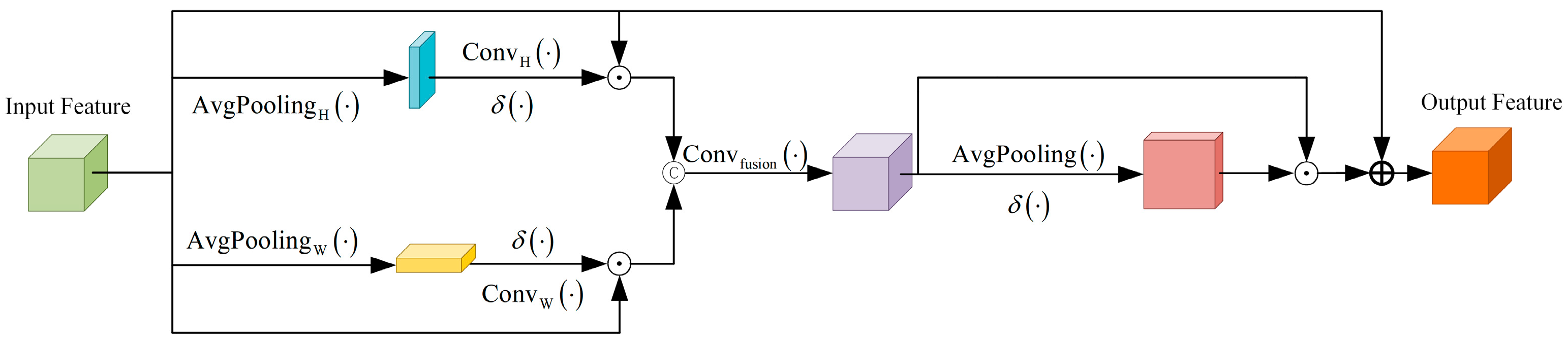
However, due to the limited receptive field of shallow CNNs, they typically capture only local spatial spectral features. Inspired by Coordinate Attention [44], we have designed the HPSCA module to achieve a more comprehensive modeling of spatial information, thereby enhancing the expressive capability of spatial features. Traditional global pooling methods process entire spatial information and compress it into channels, resulting in a loss of spatial positional information and an inability to perceive the directional characteristics of spatial structures. In contrast, HPSCA performs pooling along two spatial dimensions: height and width. This approach does not completely compress the spatial dimensions; rather, it retains responses at each position within the retained direction. Specifically, this pooling operation preserves positional information in one direction while capturing long-range dependency information in the other direction, which is utilized to guide subsequent feature weighting. The process of HPSCA is illustrated in Figure 2.

The height branch assigns a weight to each row of every channel, applying this weight across the entire feature map. This process emphasizes the significance of vertical positioning within the data. Specifically, in the height branch, we first perform average pooling along the width dimension of the input data, resulting in $F_{\mathrm{h}1}\in {ℝ}^{C\times H\times 1}$. This step captures long-range dependencies in the vertical direction while preserving information from each channel along the height axis. It takes into account not only the inter-channel relationships but also spatial positional information in the vertical orientation. Subsequently, vertical attention is generated for all channels through 2D convolution using a $1\times 1$ kernel. The Sigmoid activation function is then applied to produce an output feature map that is weighted with the input features to yield a fused feature $F_{\mathrm{h}}\in {ℝ}^{C\times H\times W}$. The formulas are as follows:

$$F_{\mathrm{h}1}={\mathrm{AvgPooling}}_{\mathrm{H}}\left(F_{2\mathrm{D}}\right)$$

(3)

$$F_{\mathrm{h}}=F_{2\mathrm{D}}·\delta \left({\mathrm{Conv}}_{\mathrm{H}}\left(F_{\mathrm{h}1}\right)\right)$$

(4)

where ${\mathrm{AvgPooling}}_{\mathrm{H}}\left(·\right)$ is pooling along the $W$ dimension. ${\mathrm{Conv}}_{\mathrm{H}}\left(·\right)$ denotes the 2D convolution with a $1\times 1$ kernel. $\delta \left(·\right)$ is defined as the Sigmoid activation function.

Similar to the height branch, the width branch assigns a weight to each column of every channel and applies this weight across the entire feature map. This process emphasizes the characteristics associated with horizontal positioning. The width branch employs average pooling along the height dimension to obtain $F_{\mathrm{w}1}\in {ℝ}^{C\times 1\times W}$, effectively capturing feature information in the horizontal direction. Subsequently, a 2D convolution with a $1\times 1$ kernel is utilized to generate horizontal attention across all channels, followed by the application of a Sigmoid activation function to derive the feature mapping. Ultimately, this results in $F_{\mathrm{w}}\in {ℝ}^{C\times H\times W}$. The formulas can be written as:

$$F_{\mathrm{w}1}={\mathrm{AvgPooling}}_{\mathrm{W}}\left(F_{2\mathrm{D}}\right)$$

(5)

$$F_{\mathrm{w}}=F_{2\mathrm{D}}·\delta \left({\mathrm{Conv}}_{\mathrm{W}}\left(F_{\mathrm{w}1}\right)\right)$$

(6)

where ${\mathrm{AvgPooling}}_{\mathrm{w}}\left(·\right)$ is pooling along the $H$ dimension. ${\mathrm{Conv}}_{\mathrm{W}}\left(·\right)$ denotes the 2D convolution with a $1\times 1$ kernel. The remaining symbols have the same meaning as the previous ones.

The two enhanced features are concatenated along the channel dimension, followed by the application of a 2D convolution using a $1\times 1$ convolution kernel to fuse these features. This process establishes distinct long-range dependencies from various spatial directions and integrates spatial information into channel attention mechanisms. It effectively incorporates global information to enhance the discriminative capabilities of the features, thereby improving the model’s perception and discrimination abilities in key areas. The formula for this procedure is provided below:

$$F_{\mathrm{hw}}={\mathrm{Conv}}_{\mathrm{fusion}}\left(\mathrm{Concat}\left(F_{\mathrm{h}},F_{\mathrm{w}}\right)\right)$$

(7)

Here, ${\mathrm{Conv}}_{\mathrm{fusion}}\left(·\right)$ denotes the 2D convolution with kernel 1. $\mathrm{Concat}\left(·\right)$ represents the concatenation of operations along the channel dimension.

To further emphasize prominent spatial features, we perform average pooling along the channel dimension of $F_{\mathrm{hw}}$, while maintaining a constant spatial dimension. The global channel information is integrated into a spatial weight template for a single channel. Subsequently, the Sigmoid activation function is employed to generate the spatial attention map, which reflects the significance of each spatial location. Finally, $F_{\mathrm{hw}}$ is feature-weighted and added to $F_{2\mathrm{D}}$. This approach preserves the original basis of feature information, thereby enhancing the attention paid to salient details. The formula is provided below:

$$F=F_{2\mathrm{D}}+F_{\mathrm{hw}}·\delta \left(\mathrm{AvgPooling}\left(F_{\mathrm{hw}}\right)\right)$$

(8)

where $\mathrm{AvgPooling}\left(·\right)$ represents pooling along the channel dimension The rest of the symbols have similar meanings as before.

Finally, the generated feature map, $F$, is expanded along the spatial dimension to produce the final output. The HPSCA module enhances features by incorporating various dimensions. This approach not only integrates global information but also facilitates a more refined enhancement of spatial features. Simultaneously, it effectively suppresses irrelevant noise, thereby providing more reliable input for subsequent modules.

2.3. Similarity Propagation Transformer Encoder

In recent years, the Transformer architecture has been extensively utilized in the field of hyperspectral image classification (HSIC) due to its exceptional capability to model long-range dependencies. Currently, there are several Transformer-based methods for HSI classification that employ multiple encoders to comprehensively extract spatial and spectral features. However, as the number of encoder layers increases, information tends to degrade during transmission. Additionally, issues related to deep attenuation may arise, which can limit the overall performance of the model. To address these challenges, we propose a Similarity Propagation Transformer Encoder comprising three key components: the Multi-head Transmission Self-attention (MHTSA) block, the Attention-MLP block, and the MLP block.

The traditional Transformer recalculates attention scores at each layer, and there exists a regularity in the semantic abstraction of attention across different layers, with higher-level attention being further refined from lower-level attention. We employ skip connections to facilitate the flow of information, allowing the attention scores from one Transformer encoder block to be transmitted to the subsequent Transformer encoder block, and thereby enhancing inter-layer information transfer.

The attention score essentially quantifies the correlation or association strength between different elements in the input sequence. Based on this principle, we add the historical attention distribution from the previous layer to the current attention scores, thereby facilitating the inheritance of cross-layer attention information. This mechanism not only alleviates information loss during inter-layer transmission but also preserves the correlations among elements from the preceding layer. As a result, it enables the model to maintain consistent focus and reinforcement on truly significant element associations across different levels.

However, the Transformer model progressively extracts features and abstracts representations from input data layer by layer. Lower layers typically focus on local information, while higher layers emphasize global or semantic information. There are significant differences between high-level semantic features and low-level semantic features; simply summing attention scores from different levels does not yield effective integration and may interfere with subsequent calculations of inter-element correlations. In light of these considerations, we have designed a nonlinear mapping module called Attention-MLP, which consists of two linear layers, a ReLU activation function and layer normalization. The Attention-MLP performs abstract modeling of the attention scores from the previous layer to accommodate deep semantic requirements. It transforms comprehensible features from lower layers into high-level abstract semantics, thereby facilitating more effective integration of low-level and high-level semantics.

All tokens are connected to a learnable classification token, $T_0^{cls}$. Then, position embedding is introduced to increase the information between locations. The input, $T_{\mathrm{in}}$, of the Transformer is obtained:

$$T_{\mathrm{in}}=\left[T_0^{cls},T_1,T_2,\cdots ,T_i\right]+{\mathrm{PE}}_{\mathrm{pos}}$$

(9)

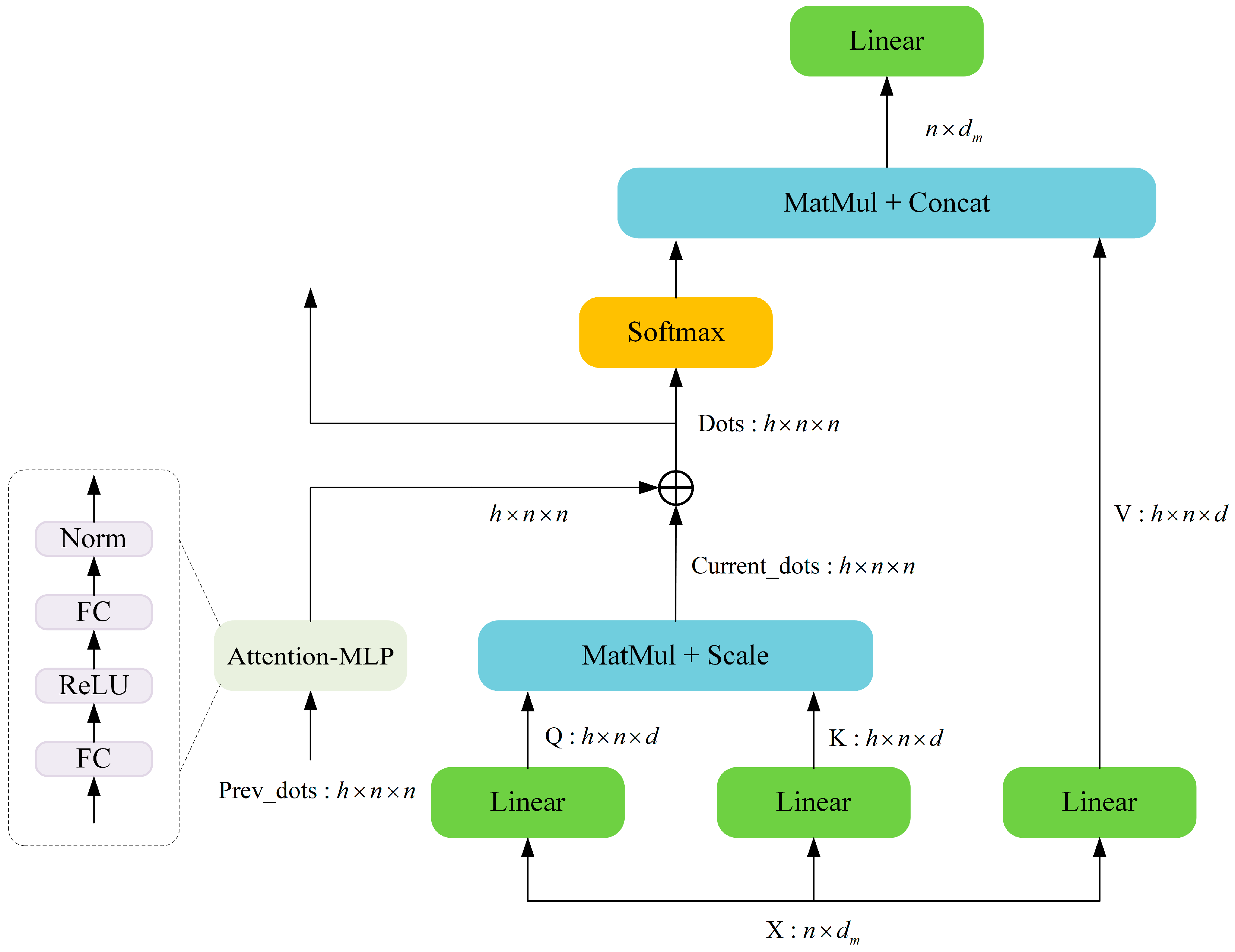
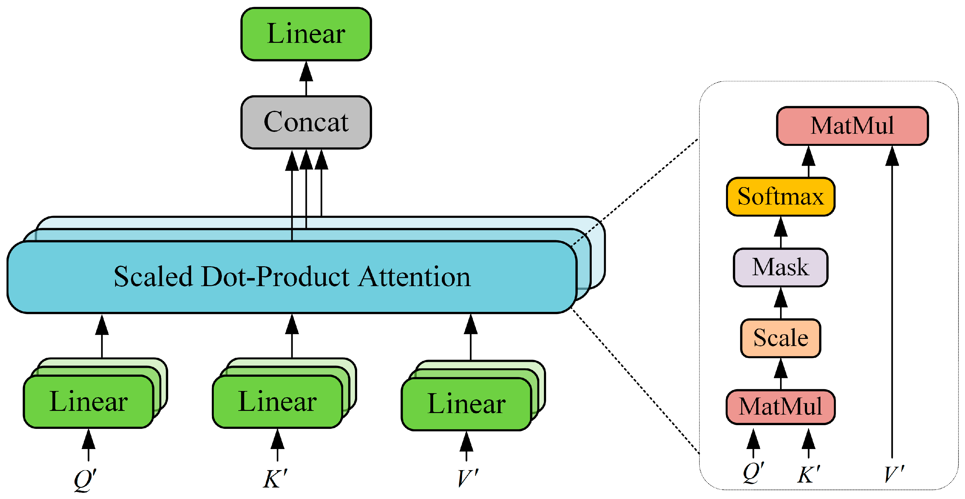
The structure of MHTSA is shown in Figure 3. MHTSA usually includes three feature inputs, namely query ($Q$), key ($K$), and value ($V$). In order to learn their different meanings, three learnable weight matrices are defined, which are $W_Q$, $W_K$, and $W_V$. The feature vector tokens are linearly mapped through these three weight matrices to obtain $Q\in {ℝ}^{n\times d}$, $K\in {ℝ}^{n\times d}$, and $V\in {ℝ}^{n\times d}$, where $n$ represents the number of feature vectors and $d$ represents their feature dimension. In order to conveniently explain the process of attention score transmission, we make the following definition of the calculation process:

$$D_{\mathrm{current}}^{\left(p\right)}={\displaystyle \frac{Q^{\left(p\right)}{\left(K^{\left(p\right)}\right)}^T}{\sqrt{d}}}$$

(10)

$${\tilde{D}}^{\left(p\right)}=\mathrm{A}-\mathrm{MLP}\left(D^{\left(p-1\right)}\right)=\mathrm{LN}\left({\mathrm{FC}}_2\left(\mathrm{ReLU}\left({\mathrm{FC}}_1\left(D^{\left(p-1\right)}\right)\right)\right)\right)$$

(11)

$$D^{\left(p\right)}=D_{\mathrm{current}}^{\left(p\right)}+{\tilde{D}}^{\left(p\right)}$$

(12)

where Equations (10)–(12) reflect the process of transferring the attention scores of layer $p-1$ to layer $p$ after the nonlinear transformation. The range of $p$ is in $\left[2,P\right]$, and $P$ denotes the maximum number of encoders in SPTE. $D_{\mathrm{current}}^p$ is the raw attention score of the $p$ layer. $\mathrm{A}-\mathrm{MLP}\left(·\right)$ performs a nonlinear transformation, where ${\mathrm{FC}}_1$ and ${\mathrm{FC}}_2$ are two fully connected layers designed to achieve nonlinear mapping of the attention scores from the previous layer, thereby enhancing feature representation. ${\tilde{D}}^{\left(p\right)}$ is obtained by performing $\mathrm{A}-\mathrm{MLP}\left(·\right)$ on the attention scores at layer $p-1$. $D^{\left(p\right)}$ represents the final attention score of the $p$ layer. For the sake of brevity, we omit the dimension transformation operation in the data processing.

After that, the Softmax function is used to convert the obtained attention scores into attention weights, and the attention weights are multiplied with $V^{\left(p\right)}$. The calculation process of each head is shown in Equation (13). Finally, all attention heads are connected, and the process is shown in Equation (14):

$${\mathrm{SA}}^{\left(p\right)}=\mathrm{Softmax}\left(D^{\left(p\right)}\right)V^{\left(p\right)}$$

(13)

$${\mathrm{MHTSA}}^{\left(p\right)}=\mathrm{Concat}\left({\mathrm{SA}}_1^{\left(p\right)},{\mathrm{SA}}_2^{\left(p\right)},\cdots ,{\mathrm{SA}}_h^{\left(p\right)}\right)W_o$$

(14)

where $h$ is the number of heads. $W_o$ is a weight parameter matrix, which is used to fuse the output of multiple heads to make the feature representation richer and more comprehensive.

The output generated by $\mathrm{MHTSA}$ is subsequently transmitted to the $\mathrm{MLP}$ block for further processing. The $\mathrm{MLP}$ block consists of two fully connected layers ($\mathrm{FC}$) and a Gaussian error linear unit ($\mathrm{GELU}$). The $\mathrm{MLP}$ block is defined as:

$$\mathrm{MLP}\left(X\right)={\mathrm{FC}}_4\left(\mathrm{GELU}\left({\mathrm{FC}}_3\left(X\right)\right)\right)$$

(15)

It is noteworthy that ${\mathrm{FC}}_3$ and ${\mathrm{FC}}_4$ in Equation (15) represent two fully connected layers within the standard MLP module.

Figure 4 illustrates the detailed architecture of the SPTE when $p=2$. In summary, the calculation process of the whole module can be summarized in more general formulas:

$$O_{\mathrm{MHTSA}}^{\left(p\right)}=\mathrm{MHTSA}\left(\mathrm{LN}\left(O^{\left(p-1\right)}\right)\right)+O^{\left(p-1\right)}$$

(16)

$$O^{\left(p\right)}=\mathrm{MLP}\left(\mathrm{LN}\left(O_{\mathrm{MHTSA}}^{\left(p\right)}\right)\right)+O_{\mathrm{MHTSA}}^{\left(p\right)}$$

(17)

where $\mathrm{LN}\left(·\right)$ stands for layer normalization, which effectively alleviates the problem of gradient disappearance or gradient explosion and improves the stability of the model. $O^{\left(p-1\right)}$ represents the input of the $p$th encoder and $O^{\left(p\right)}$ represents the output of the $p$th encoder. The input to the first encoder is $T_{\mathrm{in}}$.

In summary, the SPTE module enhances feature interaction among encoders through a similarity propagation mechanism. This mechanism utilizes attention scores from the previous layer as a form of historical memory and employs nonlinear transformations for abstraction and adaptation. As a result, the attention distributions learned in shallower layers are preserved within deeper networks, alleviating the issue of information degradation commonly encountered in deep architectures. This design not only strengthens the local detail features captured by shallow layers but also integrates global contextual information extracted from deeper layers, thereby creating a hierarchical attention enhancement that improves the model’s classification performance.

2.4. SpecFormer

Hyperspectral imaging not only provides fine spatial details but also contains rich spectral feature information. Extracting spectral features from hyperspectral images enhances the ability to recognize features, thereby improving the classification accuracy of models. The structure of the Spectral Transformer is illustrated in Figure 1. The selection of a self-attention mechanism for extracting spectral information offers several advantages.

First, Transformers possess the capability to effectively manage global dependencies within the spectral range, allowing them to capture complex nonlinear relationships between different bands more efficiently. By modeling the entire spectral sequence, Transformers can extract richer contextual information and enhance the global representational capacity of features, thus improving both the integrity and discriminative power of spectral features.

Second, Transformers can assign varying attention weights based on the significance of different features through their self-attention mechanism. Higher weights are allocated to key features that aid in distinguishing target classes, while lower attention weights are applied to noise and irrelevant information present in the spectral sequence. This mechanism enables models to autonomously amplify essential spectral features while effectively suppressing noisy bands, ultimately contributing to improved accuracy in HSI classification.

The input spectral information is $T_{\mathrm{spe}}\in {ℝ}^{1\times 1\times b}$, we connect $T_{\mathrm{spe}}$ with the learnable classification token, and perform position embedding, and finally obtain the spectral feature vector $T_{in}^{\prime }$.

$$T_{\mathrm{in}}^{\prime }=\left[T_{\mathrm{spe}0}^{cls},T_{\mathrm{spe}1},T_{\mathrm{spe}2},\cdots ,T_{\mathrm{speb}}\right]+{\mathrm{PE}}_{\mathrm{pos}}^{\prime }$$

(18)

In SpecFormer, we use traditional multi-head self-attention ($\mathrm{MHSA}$) (Figure 5) to first obtain $Q^{\prime }\in {ℝ}^{u\times d_Q}$, $K^{\prime }\in {ℝ}^{u\times d_K}$, and $V^{\prime }\in {ℝ}^{u\times d_V}$ by linearly mapping the three learnable weight matrices $W_Q^{\prime }$, $W_K^{\prime }$, and $W_V^{\prime }$ to the input. The self-attention formula is as follows:

$${\mathrm{SA}}^{\prime }=\mathrm{Softmax}\left({\displaystyle \frac{Q^{\prime }{K^{\prime }}^T}{\sqrt{d_K}}}\right)$$

(19)

where $d_K$ is the characteristic dimension of $K^{\prime }$.

$\mathrm{MHSA}$ calculates the multi-head attention values by using the same operation. Subsequently, the outputs from each attention head are merged. This process can be depicted by the following formula.

$$\mathrm{MHSA}=\mathrm{Concat}\left({\mathrm{SA}}_1^{\prime },{\mathrm{SA}}_2^{\prime },\cdots ,{\mathrm{SA}}_h^{\prime }\right)W_o^{\prime }$$

(20)

where $h$ is the number of heads and $W_o^{\prime }$ is a weight parameter matrix.

The MLP (multilayer perceptron) excels at capturing global feature interactions; however, it exhibits relatively weak capabilities in local feature extraction, often overlooking the local correlations present within spectral sequences. Additionally, the parameter count and computational complexity of MLPs are quite high. These factors can significantly limit the model’s performance. Therefore, we have opted to replace the MLP block with depthwise separable convolutions.

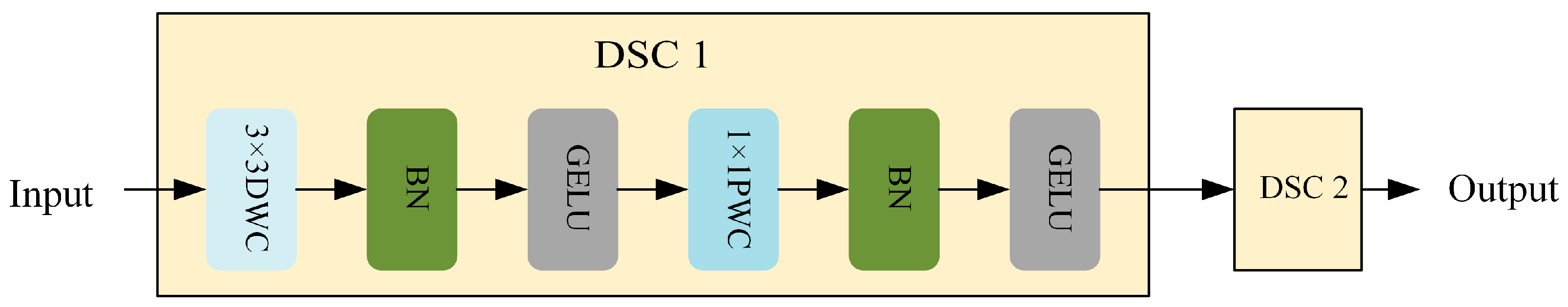
Compared to standard convolutional layers, depthwise separable convolutions require fewer parameters and exhibit lower computational complexity. However, standard convolutions possess stronger local feature extraction capabilities than their depthwise separable counterparts. To mitigate the potential accuracy loss associated with using depthwise separable convolutions, our model employs two such convolutional layers to further enhance feature representation. As illustrated in Figure 6, the Conv block is constructed from two modules of depthwise separable convolutions.

The depthwise separable convolution consists of two components: the channel-independent depthwise convolution and the cross-channel fusion pointwise convolution. Both the parameter count and the computational complexity are significantly lower than those of MLP blocks. In depthwise separable convolution, a depthwise convolution is first performed independently on each channel, followed by a pointwise convolution that executes $1\times 1$ convolutions to integrate information across channels. The formula governing this module is presented below:

$$\mathrm{DSC}=f_1\left(f_2\left(X\right)\right)$$

(21)

$$\mathrm{SpecFormer}={\mathrm{DSC}}_2\left({\mathrm{DSC}}_1\left(\mathrm{MHSA}\right)\right)$$

(22)

where $\mathrm{DSC}\left(·\right)$ is depthwise separable convolution, $f_1$ represents the composite function of pointwise convolution, BatchNorm, and GELU, and $f_2$ represents the composite function of depthwise convolution, BatchNorm, and GELU. $\mathrm{SpecFormer}$ is the output of the SpecFormer module.

2.5. Classification Head

In order to achieve the final feature classification, we have incorporated an MLP head following the concatenation of spatial and spectral features, as illustrated in Figure 1. Specifically, the MLP head constitutes the final component of the MLP architecture, which includes a LayerNorm and a fully connected layer. The LayerNorm serves to normalize the final features, thereby enhancing the stability of the model. The output dimension of the fully connected layer corresponds to the total number of target classes. Consequently, among the final output results, the class with the highest value represents the predicted classification result for that pixel.

2.6. Implementation

After data preprocessing, $X_1\in {ℝ}^{15\times 15\times 30}$ and $X_2\in {ℝ}^{1\times 1\times 30}$ are obtained. $X_1$ first performs a 3D convolution operation with 8 convolution kernels of size $3\times 3\times 3$ and then performs the 2D convolution operation with 64 convolution kernels of size $3\times 3$. Next, as the input of the HPSCA module, feature fusion is carried out to obtain 64 feature mappings with a size of $11\times 11$. Each feature map is flattened along the spatial dimension to obtain $1\times 121$ vectors. Adding learnable classification tokens and position embedding yields $T_{\mathrm{in}}\in {ℝ}^{122\times 64}$. After processing by the SPTE module, the first classification label $cls$ is the learned spatial feature, denoted as $H_{\mathrm{spa}}\in {ℝ}^{1\times 64}$. $X_2$ is used as the input of the Spectral Transformer. It obtains $T_{\mathrm{in}}^{\prime }\in {ℝ}^{31\times 64}$ by linear mapping, adding learnable classification tokens, and position embedding. After processing with SpecFormer, the first classification label corresponds to the learned spectral feature, which is denoted as $H_{\mathrm{spe}}\in {ℝ}^{1\times 64}$. Finally, the two features were concatenated into the classifier for classification.

3. Experimental Results and Analysis

In our experiments, we selected four publicly accessible HSI datasets to evaluate the performance of the proposed method. Subsequently, we will provide a detailed introduction to the information regarding these four datasets utilized in the experiment, along with a description of the configuration parameters employed. Following this, we will examine the influence of various parameters on model performance and present a quantitative analysis of classification results alongside visual outcomes and analyses. This will serve to demonstrate both the rationale behind our chosen parameters and the superiority of our model’s performance. Additionally, we conducted ablation experiments on the model to assess the specific impact of each component on classification accuracy. Finally, an analysis will be presented concerning parameter scale, number of floating-point operations, as well as training and testing times for all methods across the four datasets.

3.1. Introduction to Hyperspectral Datasets

To evaluate the classification performance of the model, we selected four HSI datasets for our experiments. These datasets include the Salinas dataset, WHU-Hi-LongKou dataset, WHU-Hi-HanChuan dataset, and the WHU-Hi-HongHu dataset.

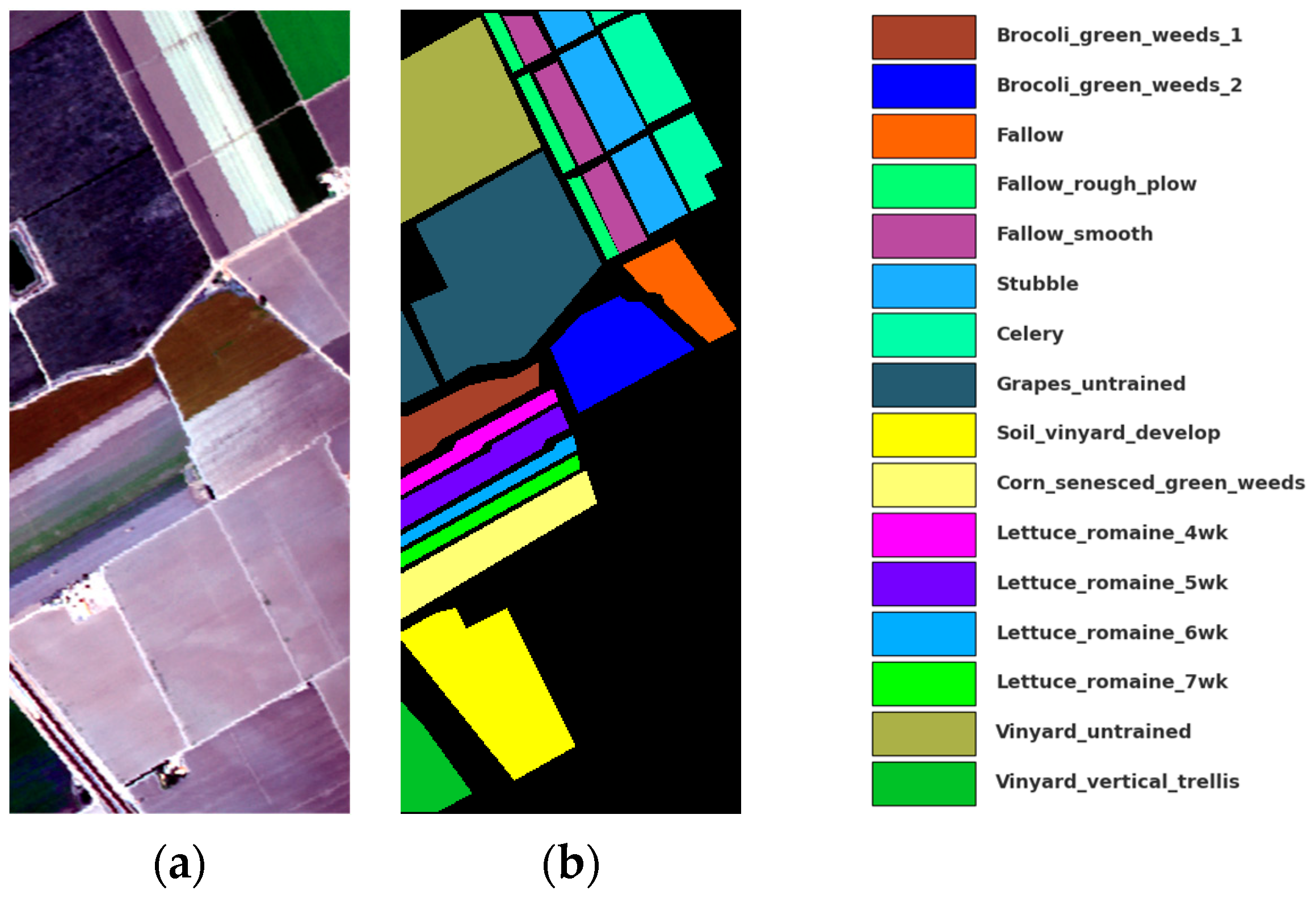
Salinas: The dataset was obtained using an Airborne Visible Infrared Imaging Spectrometer (AVIRIS) sensor in the Salinas Valley region of California. It encompasses 224 spectral bands, ranging from 0.4 microns to 2.5 microns, with a spatial resolution of 3.7 m. Due to the water absorption characteristics present in certain bands, 20 relevant bands were excluded from the dataset, resulting in a final selection of 204 bands for analysis. The dataset comprises a coverage area of 512 $\times$ 217 pixels and includes 16 distinct land cover types, as illustrated in Figure 7.

WHU-Hi-LongKou: The dataset was collected in Longkou Town, Hubei Province, China. The Headwall nano-hyperspectral imaging sensor, mounted on the DJI Matrice 600 Pro UAV platform, was utilized for data acquisition. The dataset comprises images with a resolution of 550 $\times$ 400 pixels. It covers a spectral range from 0.4 microns to 1 micron and includes a total of 270 bands. The spectral resolution is measured at 6 nm, while the spatial resolution is approximately 0.463 m, encompassing nine distinct land cover types. This information is illustrated in Figure 8.

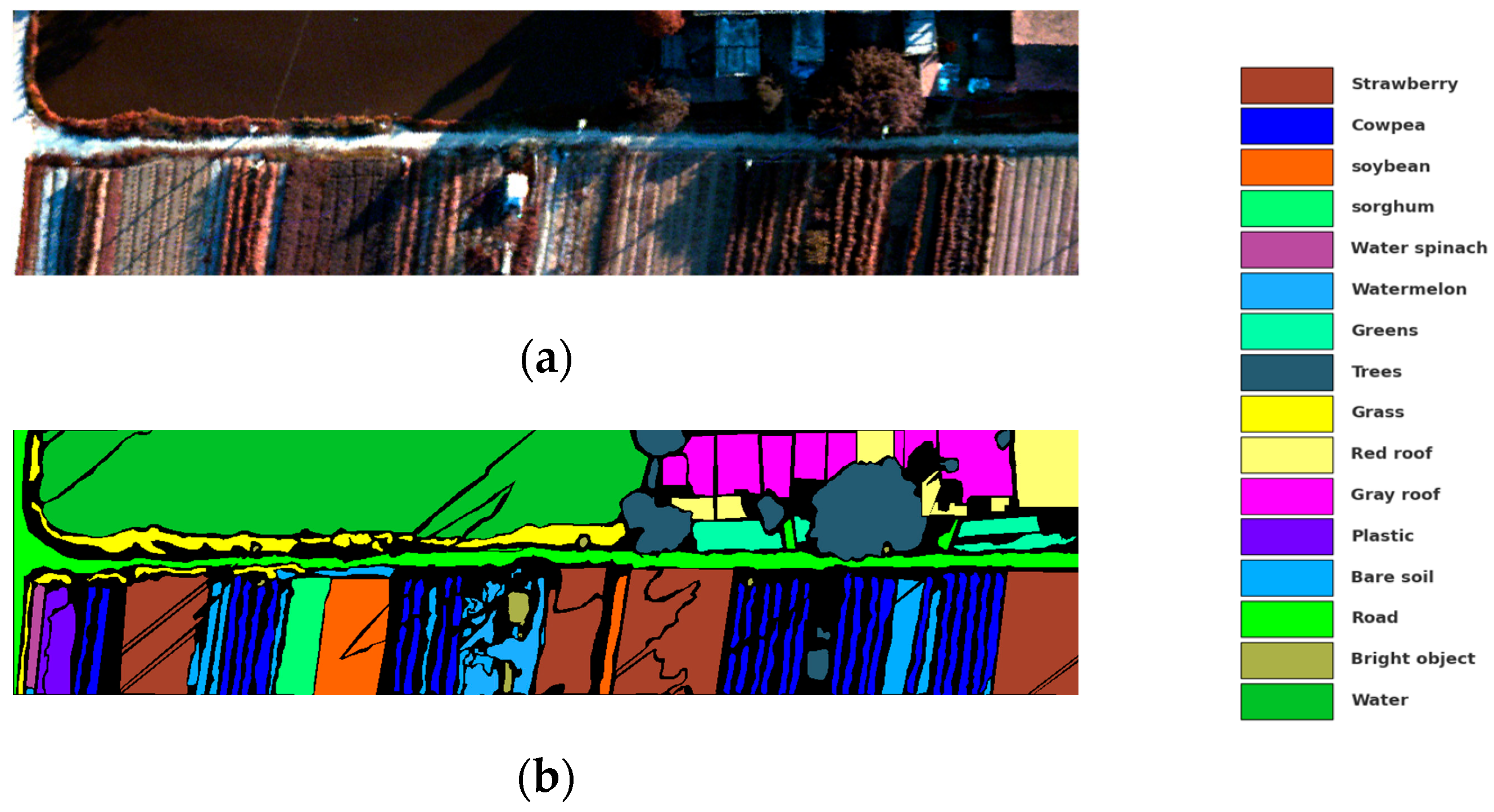
WHU-Hi-HanChuan: The dataset was collected in Hanchuan City, Hubei Province. The image data for this dataset were acquired using the Headwall nano-hyperspectral imaging sensor mounted on the Leica Aibot X6 UAV V1 platform. Each image has a resolution of 1217 $\times$ 303 pixels and encompasses spectral bands ranging from 0.4 microns to 1 micron, totaling 274 bands. The sensor features a spectral resolution of 6 nm and a spatial resolution of 0.109 m, while this dataset includes 16 distinct land cover types, as illustrated in Figure 9.

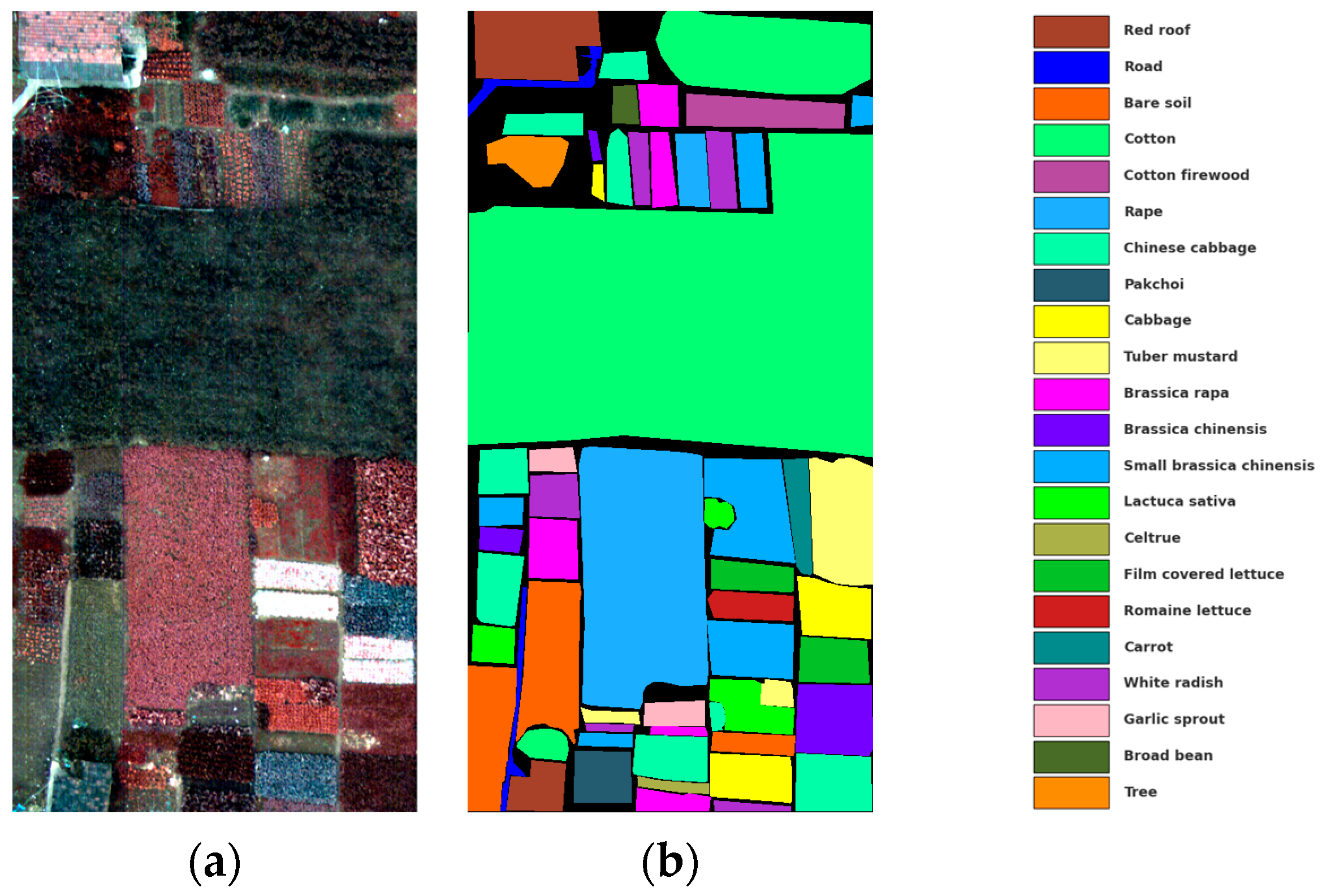
WHU-Hi-HongHu: The dataset was collected in Honghu City, Hubei Province, China, utilizing a Headwall nano-hyperspectral imaging sensor mounted on a DJI Matrice 600 Pro UAV platform. The dimensions of the images in this dataset are 940 $\times$ 475 pixels, with a spectral range extending from 0.4 microns to 1 micron, encompassing a total of 270 bands. Featuring a spectral resolution of 6 nm and a spatial resolution of 0.043 m, the dataset covers 22 distinct land cover types. This is illustrated in Figure 10.

3.2. Experimental Configuration

The classification performance of the proposed model was assessed using three quantitative metrics: overall accuracy (OA), average accuracy (AA), and kappa coefficient ($\kappa$). Specifically, OA is defined as the ratio of the number of samples accurately classified to the total number of samples in the test set. AA represents the mean classification accuracy across all classes, while $\kappa$ is closely associated with the confusion matrix and serves to measure the agreement between the classification results and true labels. Higher values for these evaluation metrics indicate superior performance.

The experimental environment is based on the Ubuntu operating system, utilizing the GeForce RTX 2080Ti GPU manufactured by NVIDIA Corporation in the United States. The programming language framework employed is Python 3.9, with PyCharm 2021.1.3 serving as the integrated development environment (IDE). We have configured the batch size to 64, selected Adaptive Moment Estimation (Adam) as the optimizer, set the learning rate at 0.001, and established a total of 100 epochs for training. For our dataset, we allocate 25 samples from each category to form the training set and another 25 samples for the validation set, while reserving the remaining samples for testing purposes. More detailed information can be founded at https://github.com/hfwiu/DBSSFormer-SP (accessed on 19 June 2025).

3.3. Classification Maps and Experimental Results

To assess the effectiveness of the proposed method, we conducted comparative trials involving our model and several representative classification methods: RSSAN [23], SPRN [45], SF [32], SSFTT [34], GAHT [36], MorphFormer [38], GSCViT [39], and MASSFormer [41]. To ensure fairness in the experimental outcomes, all methods were evaluated under identical settings across four datasets. In order to mitigate the influence of randomness on the results and enhance both reliability and stability in our evaluation process, we computed five sets of experimental averages for comparison purposes. These averages pertain to overall accuracy (OA), average accuracy (AA), and Cohen’s kappa ($\kappa$) across the four datasets; the noteworthy results are emphasized in bold.

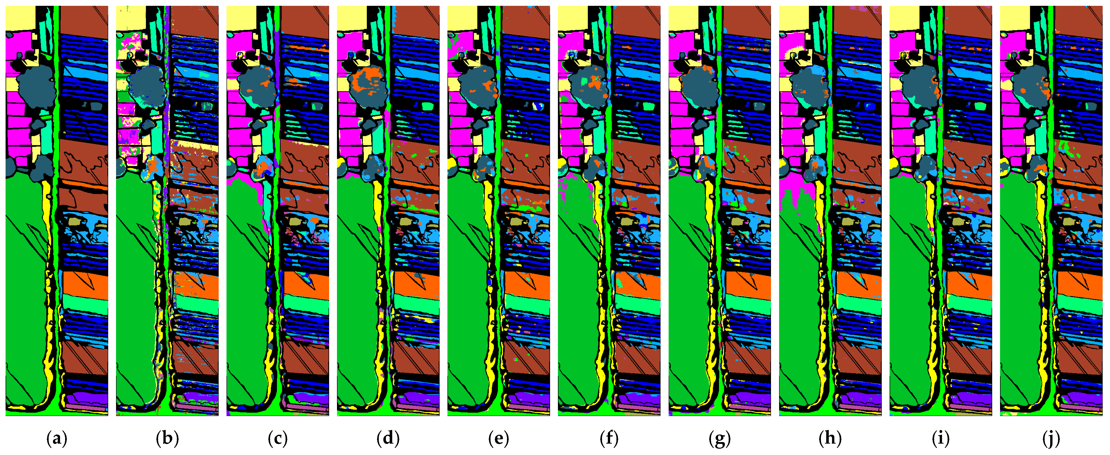
3.3.1. Classification Maps and Experimental Results for the Salinas Dataset

Table 1. OA, AA, $\kappa$, and classification results of each class for all methods on Salinas dataset (optimal results are highlighted in bold).

NO.	RSSAN	SPRN	SF	SSFTT	GAHT	MorphFormer	GSCViT	MASSFormer	Ours
1	99.71 ± 0.22	100.00 ± 0.00	99.95 ± 0.10	99.91 ± 0.18	99.99 ± 0.02	99.99 ± 0.02	99.60 ± 0.80	99.81 ± 0.21	99.95 ± 0.10
2	98.15 ± 1.09	100.00 ± 0.00	99.87 ± 0.10	99.99 ± 0.02	99.95 ± 0.10	99.99 ± 0.02	99.60 ± 0.54	99.89 ± 0.07	99.99 ± 0.01
3	97.99 ± 1.27	100.00 ± 0.00	99.60 ± 0.34	99.99 ± 0.02	100.00 ± 0.00	99.91 ± 0.19	99.82 ± 0.30	99.94 ± 0.08	100.00 ± 0.00
4	98.74 ± 1.39	99.79 ± 0.20	97.28 ± 1.63	98.84 ± 2.21	99.23 ± 0.53	98.41 ± 1.85	98.04 ± 0.70	98.72 ± 0.92	99.82 ± 0.32
5	96.50 ± 2.83	97.25 ± 1.07	96.93 ± 1.63	98.39 ± 1.20	98.33 ± 1.11	96.46 ± 3.82	99.20 ± 1.11	98.51 ± 1.28	98.68 ± 1.32
6	99.75 ± 0.38	99.84 ± 0.24	99.75 ± 0.41	99.09 ± 1.06	99.59 ± 0.60	99.81 ± 0.14	99.45 ± 1.07	98.71 ± 2.15	99.97 ± 0.03
7	95.83 ± 3.84	99.98 ± 0.05	98.80 ± 1.05	99.93 ± 0.10	99.96 ± 0.04	99.89 ± 0.10	99.78 ± 0.31	99.89 ± 0.10	99.94 ± 0.10
8	61.30 ± 19.90	86.80 ± 3.09	84.03 ± 5.21	87.27 ± 2.12	90.93 ± 2.09	89.47 ± 3.00	82.92 ± 2.20	89.01 ± 1.80	90.24 ± 4.42
9	97.11 ± 0.49	100.00 ± 0.00	99.99 ± 0.02	100.00 ± 0.00	100.00 ± 0.00	100.00 ± 0.00	99.97 ± 0.05	99.31 ± 0.33	100.00 ± 0.00
10	93.59 ± 2.55	95.67 ± 1.92	94.18 ± 2.69	95.91 ± 2.67	95.61 ± 3.81	95.67 ± 1.43	96.16 ± 3.29	95.82 ± 2.52	98.02 ± 1.45
11	98.15 ± 1.32	100.00 ± 0.00	99.41 ± 0.61	99.84 ± 0.31	100.00 ± 0.00	100.00 ± 0.00	99.96 ± 0.08	100.00 ± 0.00	100.00 ± 0.00
12	99.74 ± 0.32	99.81 ± 0.30	99.97 ± 0.03	99.60 ± 0.81	99.04 ± 0.78	99.70 ± 0.49	99.96 ± 0.04	99.98 ± 0.03	99.99 ± 0.02
13	95.22 ± 3.54	99.88 ± 0.15	99.95 ± 0.09	100.00 ± 0.00	98.98 ± 1.26	99.70 ± 0.44	97.23 ± 4.48	100.00 ± 0.00	100.00 ± 0.00
14	97.90 ± 1.89	99.94 ± 0.12	99.90 ± 0.15	99.73 ± 0.29	98.96 ± 1.06	99.75 ± 0.42	99.96 ± 0.08	99.63 ± 0.46	99.27 ± 0.58
15	84.57 ± 8.93	93.95 ± 2.12	94.67 ± 3.57	94.00 ± 2.17	94.15 ± 4.46	94.77 ± 2.80	97.24 ± 1.82	91.03± 2.10	96.57 ± 2.28
16	98.38 ± 1.07	99.92 ± 0.13	99.70 ± 0.59	98.87 ± 1.24	99.99 ± 0.02	99.97 ± 0.07	99.93 ± 0.14	99.70 ± 0.25	99.66 ± 0.24
OA (%)	88.12 ± 3.44	95.98 ± 0.82	95.20 ± 0.79	96.02 ± 0.65	96.82 ± 0.88	96.55 ± 0.62	95.55 ± 0.60	95.90 ± 0.45	97.26 ± 0.69
AA (%)	94.54 ± 1.11	98.30 ± 0.25	97.75 ± 0.33	98.21 ± 0.37	98.42 ± 0.45	98.34 ± 0.34	98.05 ± 0.29	98.12 ± 0.29	98.88 ± 0.17
$\kappa \times 100$	86.87 ± 3.75	95.52 ± 0.92	94.66 ± 0.88	95.57 ± 0.73	96.46 ± 0.98	96.16± 0.69	95.06 ± 0.67	95.43 ± 0.50	96.95 ± 0.77

presents the evaluation metrics of various methods applied to the Salinas dataset, while Figure 11 illustrates the corresponding classification maps. It is evident that our proposed method achieves remarkable classification accuracy, attaining nearly half of the highest accuracy in each category. The three evaluation metrics for our method are 97.26%, 98.88%, and 96.95%, respectively. In comparison to the second-best method, GAHT, our approach demonstrates improvements of 0.44%, 0.46%, and 0.49%. Among the other comparative methods, only RSSAN did not surpass an overall accuracy (OA) of 90%. The OAs for SPRN, SF, SSFTT, MorphFormer, GSCViT, and MASSFormer were recorded at 95.98%, 95.20%, 96.02%, 96.55%, 95.55%, and 95.90%, respectively. In the Salinas dataset, class 8, referred to as “untrained grapes”, and class 15, known as “untrained vineyards”, are both situated in the upper left region of the image and exhibit similar spectral characteristics. This overlap complicates the differentiation between these two classes. Both SF and GSCViT demonstrate significant areas of classification errors within the gray zone corresponding to Grapes_untrained. In contrast, the classification maps produced by our method show improved performance in this area, featuring relatively distinct boundaries.

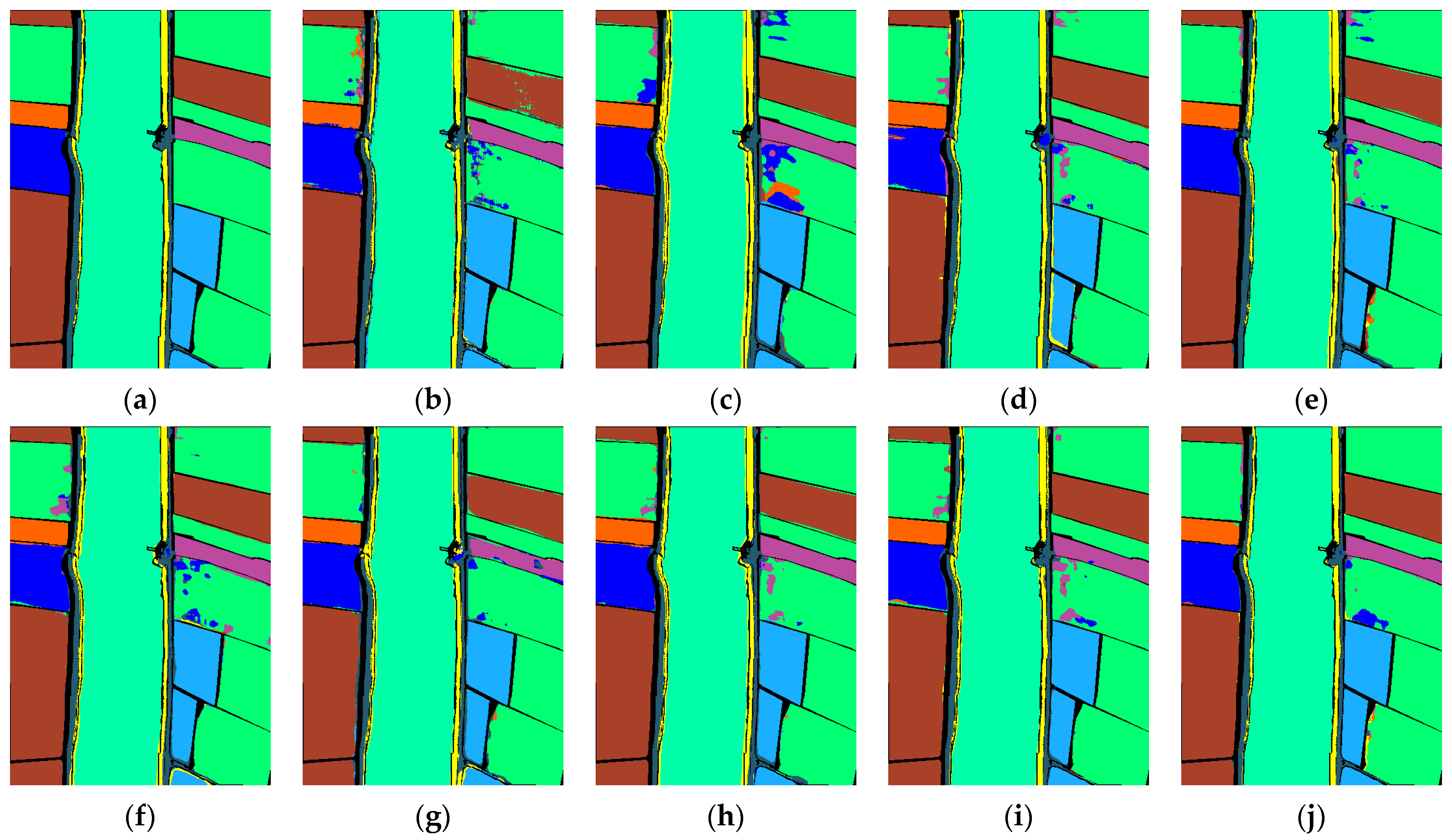
3.3.2. Classification Maps and Experimental Results for the LongKou Dataset

Table 2. OA, AA, $\kappa$, and classification results of each class for all methods on LongKou dataset (optimal results are highlighted in bold).

NO.	RSSAN	SPRN	SF	SSFTT	GAHT	MorphFormer	GSCViT	MASSFormer	Ours
1	97.74 ± 1.22	99.25 ± 0.20	99.50 ± 0.14	99.21 ± 0.45	99.59 ± 0.08	97.83 ± 1.40	99.10 ± 0.59	99.73 ± 0.18	99.61 ± 0.56
2	91.12 ± 4.85	98.01 ± 1.02	93.91 ± 1.51	98.63 ± 0.73	96.62 ± 1.60	97.55 ± 1.37	98.61 ± 0.99	97.15 ± 2.26	98.19 ± 0.79
3	94.18 ± 2.70	99.58 ± 0.17	99.55 ± 0.65	99.77 ± 0.34	99.50 ± 0.34	99.62 ± 0.42	99.72 ± 0.23	99.34 ± 0.48	98.79 ± 0.67
4	90.90 ± 3.14	92.64 ± 3.25	94.19 ± 2.35	96.57 ± 1.52	93.88 ± 1.30	95.30 ± 3.21	96.70 ± 1.01	97.12 ± 0.62	97.12 ± 1.24
5	93.55 ± 2.52	99.24 ± 0.44	98.61 ± 1.67	98.88 ± 0.66	98.86 ± 0.86	95.28 ± 5.80	98.42 ± 2.19	98.19 ± 1.05	99.82 ± 0.18
6	95.32 ± 2.18	95.57 ± 3.12	97.50 ± 2.31	98.36 ± 0.97	92.70 ± 3.72	96.07 ± 1.82	97.72 ± 1.03	99.16 ± 0.83	99.61 ± 0.23
7	98.46 ± 1.16	95.20 ± 2.37	99.68 ± 0.35	98.07 ± 1.06	96.91 ± 1.74	98.14 ± 1.48	97.00 ± 1.53	98.51 ± 1.68	99.92 ± 0.09
8	90.00 ± 4.26	91.32 ± 1.89	93.43 ± 2.56	93.99 ± 2.56	89.25 ± 3.54	88.95 ± 2.53	91.87 ± 0.63	90.52 ± 3.33	96.01 ± 2.21
9	89.14 ± 7.44	89.25 ± 2.12	95.07 ± 2.72	90.85 ± 3.30	92.28 ± 3.60	90.38 ± 4.24	90.77 ± 3.10	96.25 ± 1.08	98.35 ± 1.00
OA (%)	94.82 ± 1.77	95.09 ± 1.24	97.23 ± 0.63	97.55 ± 0.56	95.86 ± 0.96	96.51 ± 0.64	97.10 ± 0.46	97.94 ± 0.73	98.72 ± 0.35
AA (%)	93.38 ± 2.41	95.56 ± 0.91	96.83 ± 0.60	97.15 ± 0.51	95.51 ± 1.14	95.46 ± 1.19	96.66 ± 0.57	97.33 ± 0.60	98.60 ± 0.21
$\kappa \times 100$	93.27 ± 2.28	93.64 ± 1.59	96.39 ± 0.81	96.80 ± 0.72	94.62 ± 1.23	95.45 ± 0.83	96.22 ± 0.60	97.31 ± 0.95	98.32 ± 0.46

presents the classification performance indicators of various methods applied to the LongKou dataset, while Figure 12 illustrates the corresponding visual classification maps. Our proposed method demonstrates exceptional classification performance on this dataset, achieving OA, AA, and $\kappa$ of 98.72%, 98.60%, and 98.32%, respectively. In comparison to the second-best method, MASSFormer, our approach shows improvements of 0.78%, 1.27%, and 1.01% across these three evaluation metrics.

The overall accuracies for SPRN, RSSAN, SF, SSFTT, GAHT, MorphFormer, and GSCViT are recorded at 95.09%, 94.82%, 97.23%, 97.55%, 95.86%, 96.51%, and 97.10%, respectively; our proposed model surpasses these methods by margins of 3.63%, 3.90%, 1.49%, 1.17%, 2.89%, 2.21%, and 1.62%. Furthermore, in terms of category accuracy, our method consistently achieves over a remarkable threshold of more than 96% across all categories.

In the classification maps of the LongKou dataset, all comparison methods exhibit varying degrees of classification errors at the boundary between class 1 and class 2. Notably, even the second-best performing method, MASSFormer, encounters this issue. In contrast, our method demonstrates a remarkably clear delineation at the boundaries of these two categories. Furthermore, in classes 8 (“Roads and houses”) and 9 (“mixed weed”), our method’s classification maps are distinguished by their well-defined boundaries. These two classes are spatially adjacent with interconnected boundaries, making them particularly susceptible to classification errors.

3.3.3. Classification Maps and Experimental Results for the HanChuan Dataset

Table 3. OA, AA, $\kappa$, and classification results of each class for all methods on HanChuan dataset (optimal results are highlighted in bold).

NO.	RSSAN	SPRN	SF	SSFTT	GAHT	MorphFormer	GSCViT	MASSFormer	Ours
1	74.75 ± 9.65	95.10 ± 1.22	91.28 ± 2.60	89.90 ± 2.64	91.48 ± 2.17	89.99 ± 3.25	90.95 ± 2.62	91.20 ± 2.43	92.66 ± 2.67
2	68.70 ± 7.22	80.28 ± 2.50	86.85 ± 4.26	81.55 ± 3.86	80.82 ± 3.79	85.77 ± 3.43	87.69 ± 1.62	83.89 ± 4.78	89.97 ± 2.90
3	72.46 ± 9.56	89.23 ± 3.53	95.47 ± 0.58	93.58 ± 2.14	88.61 ± 3.72	93.03 ± 4.66	93.00 ± 4.57	93.36 ± 2.02	92.16 ± 4.74
4	93.28 ± 2.79	98.93 ± 0.56	98.19 ± 1.87	97.03 ± 0.36	97.63 ± 1.14	99.07 ± 0.66	98.33 ± 1.22	98.48 ± 1.58	98.76 ± 1.34
5	94.90 ± 6.55	99.98 ± 0.03	99.77 ± 0.34	98.49 ± 1.89	99.57 ± 0.30	98.24 ± 2.10	98.90 ± 1.35	99.72 ± 0.44	98.57 ± 1.72
6	60.22 ± 9.39	66.92 ± 5.22	85.09 ± 3.83	84.84 ± 7.68	80.52 ± 7.48	84.89 ± 5.65	87.25 ± 2.72	81.61 ± 2.21	83.60 ± 7.45
7	83.91 ± 7.81	97.75 ± 0.98	92.06 ± 1.64	94.65 ± 1.80	94.36 ± 2.22	95.78 ± 2.32	94.02 ± 3.37	92.14 ± 5.75	94.74 ± 1.48
8	55.30 ± 8.67	59.73 ± 8.93	75.81 ± 5.95	77.26 ± 4.16	73.17 ± 3.03	79.84 ± 3.23	72.24 ± 9.25	81.85 ± 4.02	84.02 ± 4.61
9	52.64 ± 14.15	48.15 ± 8.93	79.12 ± 1.69	88.49 ± 3.37	81.40 ± 2.18	86.98 ± 3.32	82.12 ± 6.97	88.72 ± 2.67	88.11 ± 4.07
10	83.15 ± 11.05	95.52 ± 1.12	97.81 ± 1.14	97.14 ± 0.93	93.23 ± 1.94	94.64 ± 1.66	97.00 ± 1.61	97.05 ± 1.68	96.91 ± 1.97
11	63.49 ± 21.49	95.70 ± 1.90	93.28 ± 2.23	94.81 ± 3.98	89.85 ± 2.71	95.90 ± 1.92	91.11 ± 4.03	93.68 ± 2.53	96.63 ± 0.93
12	74.84 ± 11.15	69.68 ± 2.01	95.05 ± 2.35	94.44 ± 3.73	92.32 ± 1.12	95.31 ± 3.08	96.09 ± 3.13	94.10 ± 3.80	92.09 ± 5.85
13	52.24 ± 13.75	50.06 ± 7.96	81.01 ± 3.05	78.90 ± 7.93	69.79 ± 7.02	84.35 ± 3.72	80.28 ± 1.46	80.67 ± 2.72	82.67 ± 4.03
14	54.86 ± 8.02	68.14 ± 10.04	72.71 ± 6.28	81.50 ± 6.87	79.50 ± 4.05	84.94 ± 2.80	85.04 ± 9.08	87.04 ± 3.46	86.96 ± 3.12
15	84.53 ± 6.90	82.63 ± 2.82	91.25 ± 2.70	96.63 ± 2.30	92.52 ± 5.10	95.05 ± 4.88	92.43 ± 7.10	96.24 ± 3.14	95.62 ± 1.79
16	93.90 ± 5.58	95.89 ± 0.93	97.37 ± 1.76	98.41 ± 1.70	94.02 ± 4.95	98.07 ± 1.92	96.17 ± 3.05	98.44 ± 0.76	98.96 ± 0.84
OA (%)	75.42 ± 2.38	85.37 ± 1.36	90.16 ± 0.92	90.79 ± 1.31	87.91 ± 1.87	91.67 ± 1.40	90.37 ± 1.71	91.86 ± 0.71	93.20 ± 0.55
AA (%)	72.70 ± 3.68	80.86 ± 1.02	89.51 ± 0.39	90.48 ± 0.59	87.42 ± 1.01	91.37 ± 0.68	90.16 ± 0.94	91.14 ± 0.37	92.03 ± 0.77
$\kappa \times 100$	71.54 ± 2.70	83.00 ± 1.55	88.54 ± 1.05	89.28 ± 1.49	85.96 ± 2.10	90.30 ± 1.60	88.80 ± 1.97	90.51 ± 0.81	92.06 ± 0.64

presents the classification performance metrics obtained by various methods on the HanChuan dataset, while Figure 13 illustrates the visual classification results. The HanChuan dataset utilized in this study contains numerous shadowed areas within the images, which pose significant challenges to the classification task. The overall accuracy (OA) of two CNN-based methods, namely RSSAN and SPRN, falls below 90%. Despite CNNs possessing robust local feature extraction capabilities, they struggle to effectively capture global features. This limitation adversely impacts their performance in classification tasks, resulting in a significantly inferior classification effect compared to the Transformer-based methods. Among the Transformer-based comparison methods, MASSFormer demonstrates superior classification performance, with the OA, average accuracy (AA), and kappa coefficient ($\kappa$) reaching 91.86%, 91.14%, and 90.51%, respectively. Our proposed method achieves even better classification outcomes with OA, AA, and $\kappa$ recorded at 93.20%, 92.03%, and 92.06%, respectively—an improvement of 1.34% over MASSFormer. In examining the classification maps for the HanChuan dataset, it is evident that category eight (“Tree”) poses considerable identification challenges; nearly all comparative methods exhibit errors in classifying this category. Notably, similar to findings from the LongKou dataset analysis, our classification map maintains clarity at class boundaries across different categories. Conversely, confusion errors are observed in both light blue and dark blue regions of the image’s lower right section as identified by MASSFormer et al., specifically between class two (“Cowpea”) and class thirteen (“Bare soil”).

3.3.4. Classification Maps and Experimental Results for the HongHu Dataset

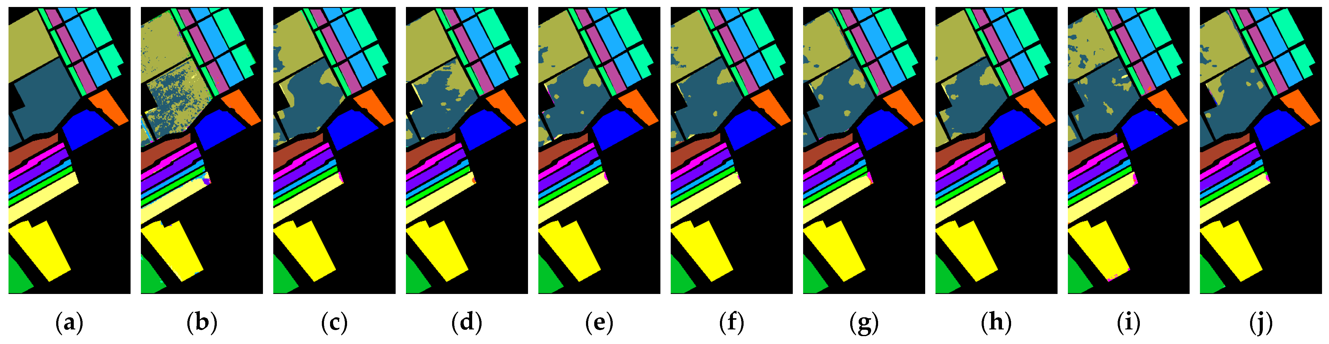
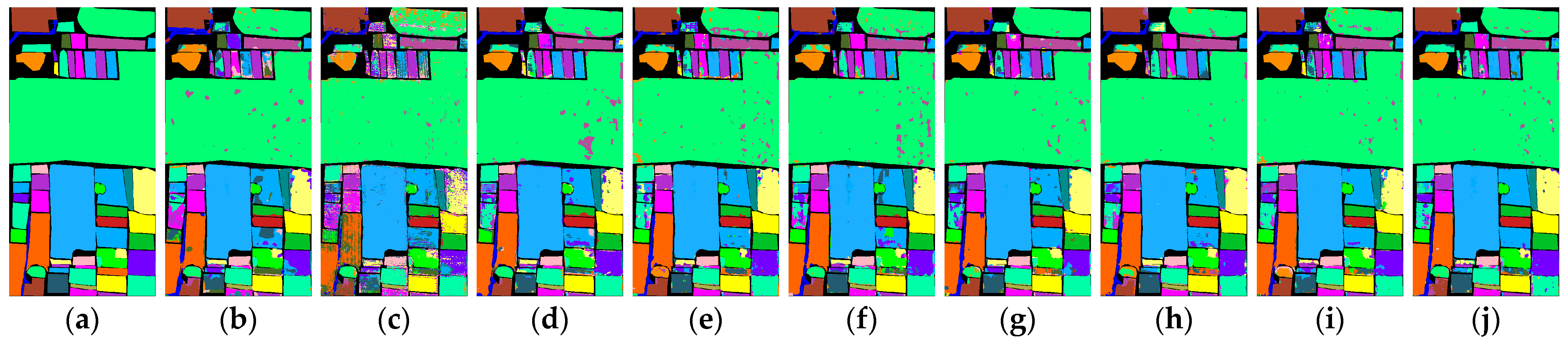
It can be observed from

Table 4. OA, AA, $\kappa$, and classification results of each class for all methods on HongHu dataset (optimal results are highlighted in bold).

No.	RSSAN	SPRN	SF	SSFTT	GAHT	MorphFormer	GSCViT	MASSFormer	Ours
1	83.94 ± 8.34	82.45 ± 5.16	94.27 ± 1.89	94.89 ± 1.39	93.30 ± 2.35	92.70 ± 2.52	92.33 ± 1.68	95.52 ± 0.42	94.69 ± 2.51
2	80.84 ± 8.36	85.29 ± 2.57	88.50 ± 5.74	93.43 ± 2.92	93.73 ± 3.07	92.26 ± 6.49	96.61 ± 3.16	94.76 ± 2.56	96.03 ± 1.79
3	74.75 ± 11.21	81.93 ± 1.75	82.87 ± 1.30	87.85 ± 1.26	86.11 ± 2.06	86.35 ± 0.84	85.70 ± 3.90	84.48 ± 2.16	87.83 ± 2.39
4	91.81 ± 1.48	95.15 ± 1.69	95.35 ± 1.85	94.65 ± 1.08	96.75 ± 1.07	97.42 ± 0.69	96.69 ± 2.27	97.04 ± 1.41	97.00 ± 1.33
5	86.73 ± 7.71	93.49 ± 1.87	94.83 ± 1.95	94.22 ± 1.76	95.03 ± 1.07	95.96 ± 2.28	96.90 ± 1.58	94.15 ± 2.93	95.02 ± 1.92
6	87.79 ± 3.34	91.64 ± 0.45	94.20 ± 3.06	95.21 ± 1.58	92.43 ± 0.93	93.69 ± 0.85	94.35 ± 2.15	95.91 ± 2.00	94.58 ± 1.24
7	54.29 ± 10.05	64.03 ± 3.37	78.98 ± 4.74	78.53 ± 6.55	75.79 ± 4.47	83.37 ± 4.75	82.39 ± 4.57	81.82 ± 2.54	84.60 ± 3.32
8	61.81 ± 4.51	61.93 ± 3.72	86.85 ± 3.54	89.15 ± 4.88	91.46 ± 3.25	89.28 ± 5.63	88.60 ± 6.31	86.44 ± 3.09	92.49 ± 1.75
9	90.68 ± 2.62	92.92 ± 1.85	96.21 ± 1.33	95.98 ± 2.11	95.35 ± 0.81	95.27 ± 2.04	96.64 ± 1.17	97.17 ± 2.38	96.44 ± 2.82
10	68.07 ± 7.04	78.42 ± 2.58	82.65 ± 2.86	90.45 ± 3.20	89.45 ± 1.97	93.07 ± 2.12	90.68 ± 2.84	89.79 ± 5.20	92.43 ± 1.30
11	50.44 ± 12.62	59.32 ± 5.40	86.28 ± 3.70	88.87 ± 5.79	84.36 ± 3.33	86.91 ± 1.29	87.97 ± 4.59	85.88 ± 2.33	87.28 ± 3.88
12	66.43 ± 9.69	69.61 ± 3.69	72.99 ± 3.22	82.65 ± 4.06	81.69 ± 2.67	83.47 ± 3.74	84.97 ± 3.38	86.07 ± 2.73	89.35 ± 1.69
13	56.60 ± 8.11	65.64 ± 6.93	72.08 ± 5.42	79.70 ± 3.11	78.95 ± 3.52	79.65 ± 4.20	81.14 ± 2.16	76.08 ± 3.96	83.39 ± 2.73
14	80.06 ± 7.20	85.81 ± 7.71	93.84 ± 3.69	94.83 ± 4.34	93.75 ± 1.38	97.18 ± 1.32	96.71 ± 1.88	97.10 ± 1.11	97.20 ± 1.87
15	87.96 ± 7.30	99.58 ± 0.40	98.68 ± 0.88	99.83 ± 0.22	99.75 ± 0.17	99.75 ± 0.40	99.71 ± 0.31	97.96 ± 1.79	99.03 ± 1.03
16	87.03 ± 7.98	91.04 ± 1.61	93.11 ± 3.00	97.60 ± 0.56	96.02 ± 1.33	96.42 ± 2.24	99.38 ± 0.60	96.66 ± 3.01	96.61 ± 2.11
17	91.95 ± 6.36	94.04 ± 3.86	93.95 ± 4.29	98.83 ± 0.58	96.59 ± 2.26	96.04 ± 2.02	97.22 ± 3.77	97.05 ± 3.24	99.58 ± 0.42
18	84.92 ± 2.88	97.38 ± 1.58	95.99 ± 1.39	96.67 ± 2.93	97.76 ± 1.31	97.20 ± 1.78	96.24 ± 2.16	96.34 ± 2.32	97.95 ± 2.14
19	79.71 ± 8.74	90.20 ± 1.74	92.24 ± 2.50	93.89 ± 2.26	90.30 ± 1.23	91.78 ± 0.91	92.76 ± 3.23	96.61 ± 1.25	97.49 ± 0.32
20	81.43 ± 10.55	87.47 ± 13.11	94.91 ± 3.24	97.92 ± 1.31	97.31 ± 1.37	98.24 ± 0.87	98.87 ± 0.63	98.88 ± 0.73	98.95 ± 0.92
21	90.81 ± 3.08	92.68 ± 11.48	96.96 ± 3.63	99.28 ± 0.87	97.20 ± 4.35	98.98 ± 1.45	96.95 ± 3.63	97.45 ± 2.11	99.83 ± 0.16
22	86.39 ± 4.88	98.98 ± 0.91	98.75 ± 1.13	98.54 ± 1.01	99.20 ± 0.74	99.20 ± 0.89	98.70 ± 0.77	98.97 ± 0.46	99.12 ± 0.76
OA (%)	81.86 ± 1.89	86.83 ± 0.56	90.68 ± 1.25	92.04 ± 0.62	91.93 ± 0.53	93.18 ± 0.61	93.06 ± 1.28	93.02 ± 0.60	93.94 ± 0.36
AA (%)	78.38 ± 2.81	84.50 ± 0.35	90.20 ± 0.70	92.86 ± 0.09	91.92 ± 0.55	92.92 ± 0.77	93.25 ± 0.63	92.82 ± 0.30	94.40 ± 0.34
$\kappa \times 100$	77.53 ± 2.34	83.55 ± 0.66	88.35 ± 1.52	90.05 ± 0.75	89.88 ± 0.65	91.44 ± 0.76	91.30 ± 1.56	91.23 ± 0.73	92.39 ± 0.44

and Figure 14 that, in the HongHu dataset, our method achieved superior classification results, with OA, AA, and $\kappa$ recorded at 93.94%, 94.40%, and 92.39%, respectively. The HongHu dataset presents significant challenges due to the diversity of crops, including various varieties of the same crop cultivated within the same region. In comparison to MorphFormer, which attained the highest classification accuracy among all evaluated methods, our approach improved upon three key metrics by margins of 0.76%, 1.48%, and 0.95%. Notably, our method surpassed a classification accuracy of over 90% across 17 out of the total 22 categories assessed. Conversely, two CNN-based methods demonstrated lower performance levels; specifically, SPRN achieved an OA of only 86.83%, while RSSAN recorded an OA of merely 81.86%. Among the Transformer-based methodologies, SF, SSFTT, GAHT, GSCViT, and MASSFormer yielded OAs of 90.68%, 92.04%, 91.93%, 93.18%, and approximately 93%, respectively. The OA of our model is 3.26%, 1.9%, 2.01%, 0.76%, 0.88%, and 0.92% higher than those of these methods, respectively.

In the classification maps of the HongHu dataset, SSFTT, GAHT, MorphFormer, GSCViT, and MASSFormer exhibit significant areas of classification errors in the green region at the top of the image. In contrast, our method demonstrates a relatively clean representation in this area of the classification map. This further substantiates that our approach achieves exceptional classification performance.

3.4. T-SNE Visualization

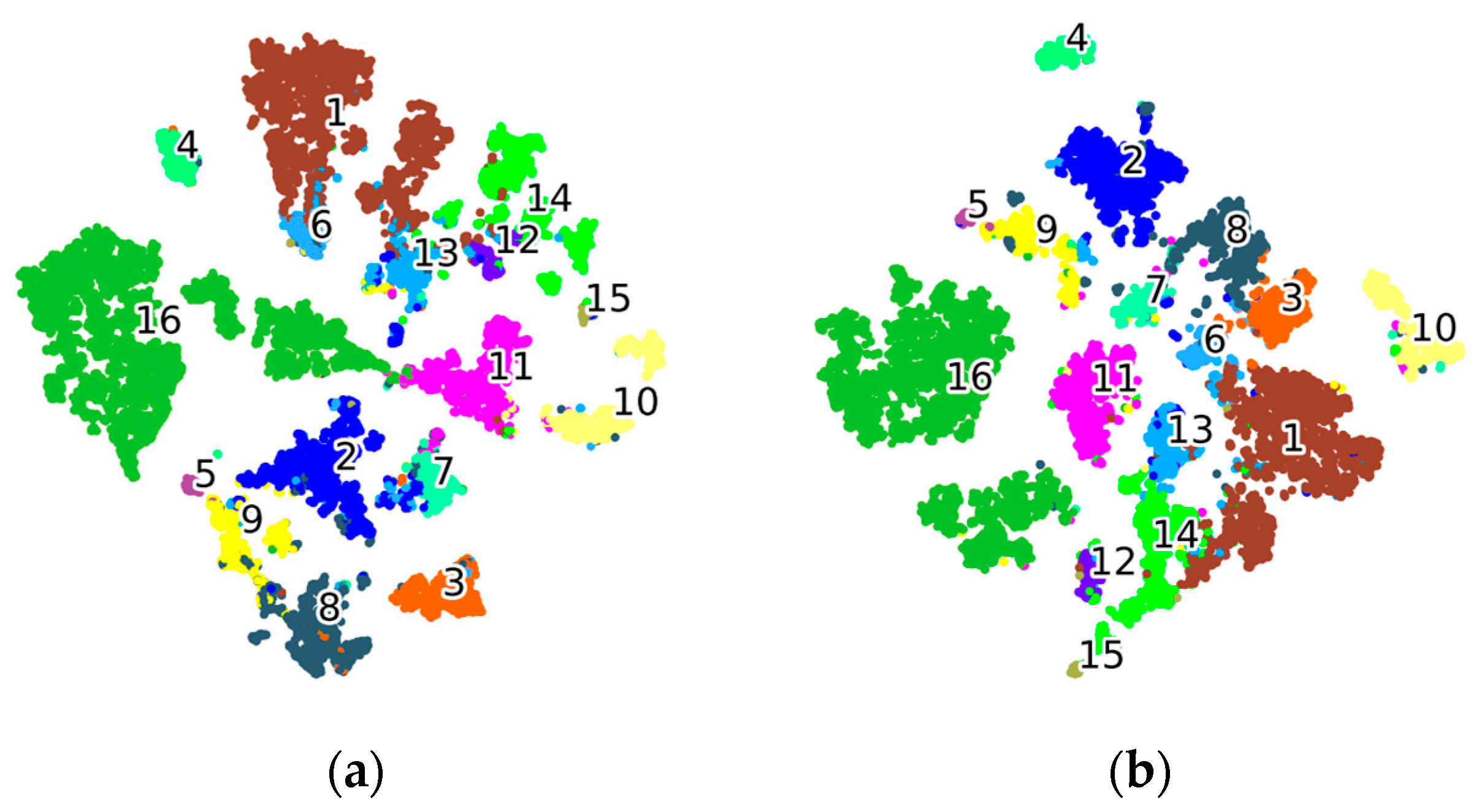
In order to better assess the effectiveness of the model, we generated t-distributed stochastic neighbor embedding (T-SNE) visualizations of the patterned features obtained by DBSSFormer-SP on the HanChuan dataset. In this dataset, MASSFormer achieved the second-best classification performance. Therefore, we compared the visualization results of DBSSFormer-SP with those of MASSFormer.

As illustrated in Figure 15, it is evident that our method effectively clusters samples of different categories within their respective subspaces in the T-SNE visualization. The boundaries are more distinct, and the overlapping regions have been significantly reduced. The intra-class compactness of DBSSFormer-SP surpasses that of MASSFormer, with most categories exhibiting a relatively compact cluster distribution and fewer outliers. This indicates that our model demonstrates greater consistency in feature extraction for similar samples. In contrast, the second and seventh classes of MASSFormer show noticeable confusion states. Our proposed method exhibits fewer inter-class errors. The comparison with MASSFormer highlights that our approach possesses superior feature discrimination and expressive capabilities.

3.5. Parametric Analysis

(1)

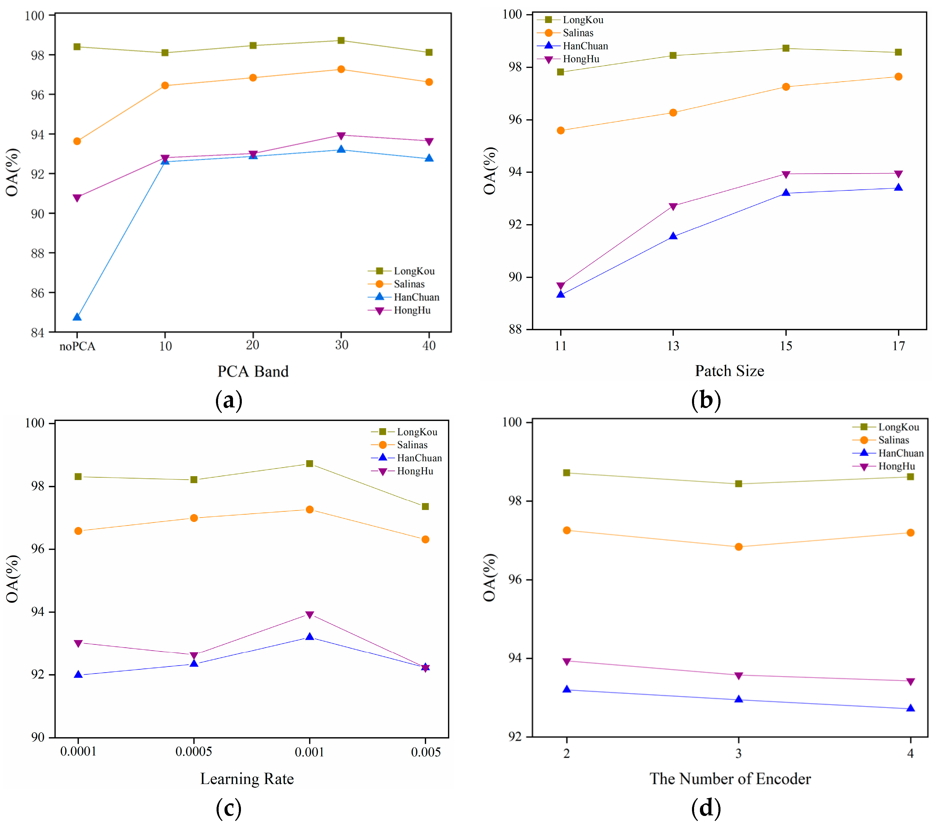
PCA band: The impact of the number of PCA bands on the experimental results cannot be overlooked. If dimensionality reduction is performed using PCA based on the information ratio, it may still retain a significant number of spectral bands. For large datasets such as LongKou, HanChuan, and HongHu, retaining a substantial number of spectral bands can consume considerable memory space and lead to increased training and testing times for a model. Therefore, we propose a set of fixed values for experimentation in order to select optimal parameters. Furthermore, we also took into account the experimental results obtained without performing PCA. The results are illustrated in Figure 16a. It is evident that the classification performance of the model is significantly poor without applying PCA for dimensionality reduction. This is particularly pronounced in the HanChuan dataset, where the overall accuracy falls below 90%. Following the dimensionality reduction through PCA, as the number of bands increases, the OA for the LongKou dataset, Salinas dataset, HanChuan dataset, and HongHu dataset initially rise before subsequently declining. The maximum OA for all four datasets occurs when the number of bands is set to 30: 98.72% for LongKou, 97.26% for Salinas, 93.2% for HanChuan, and 93.94% for HongHu. Consequently, we have determined to set the number of PCA bands to 30 in our analyses.

(2)

Patch size: The size of the patch window significantly influences the spatial perception capabilities of the model. While smaller patch sizes can effectively reduce computational complexity, they may fail to capture essential information fully. Conversely, larger patch sizes facilitate the acquisition of richer contextual information, thereby enhancing performance. However, excessively large window sizes may introduce redundant data, which can diminish the model’s discriminative power. To assess the impact of various patch sizes on classification performance, multiple sets of patch dimensions were established for experiments across four datasets while keeping other experimental parameters constant. Figure 16b illustrates the variation in overall accuracy (OA), corresponding to the different patch sizes across these datasets. As the window size increases, OA for the Salinas dataset consistently rises; at a window size of 17, OA reaches 97.65%, marking optimal classification performance. For both the HanChuan and HongHu datasets, OA initially increases with increasing window size before stabilizing. At a window size of 15, OAs are recorded at 93.2% and 93.94%, respectively. In contrast, for the LongKou dataset, OA first ascends and then descends as window size grows; it achieves its peak value of 98.72% when set to a window size of 15. When employing a patch size of 17, numerous parameters are introduced that escalate computational costs significantly. Therefore, we have opted to maintain a patch size of 15 to ensure adequate classification accuracy while preserving low model complexity.

(3)

Learning rate: The learning rate is a crucial hyperparameter in model training. Establishing an appropriate learning rate can significantly accelerate the convergence process, facilitate faster attainment of the global optimal solution, and enhance overall model performance. We select the optimal learning rate from a range of candidate values. Figure 16c illustrates the impact of various learning rates on overall accuracy (OA). It is evident that as the learning rate increases, so does the OA across all four datasets. The OA reaches its peak when the learning rate is set to 0.001. Beyond this point, although the learning rate continues to rise, there is a noticeable decline in OA for all four datasets to varying degrees. Consequently, we have determined that a learning rate of 0.001 will be employed for our model.

(4)

Number of encoders: The number of distinct Transformer encoders can significantly influence classification performance. We aim to utilize varying numbers of encoder blocks in SPTE and examine how the model’s classification performance evolves as the number of encoders increases. As illustrated in Figure 16d, it is evident that, when the number of encoders is set to 2, optimal classification accuracy is achieved across all four datasets. As the number of encoders rises, the overall accuracy (OA) on these datasets exhibits minor fluctuations within a small amplitude.

Figure 16. Impact of different parameters on OA. (a) PCA band. (b) Patch size. (c) Learning rate. (d) The number of encoders.

Figure 16. Impact of different parameters on OA. (a) PCA band. (b) Patch size. (c) Learning rate. (d) The number of encoders.

3.6. Ablation Experiments

3.6.1. Ablation Experiment of Similarity Propagation

To validate the effectiveness of the proposed similarity propagation mechanism in alleviating information degradation and deep attenuation in deep networks, we designed ablation experiments under different encoder depths. Specifically, we constructed network architectures with varying numbers of Transformer encoder layers (two, three, and four layers) across four hyperspectral datasets. We compared the impact on model classification performance based on whether or not the similarity propagation mechanism was incorporated (denoted as SP for models that include this mechanism and Non-SP for those that do not).

All experiments were conducted under the same conditions, repeated five times to obtain average values. The experimental results are presented in

Table 5. The quantitative results of experiments conducted on four datasets using varying numbers of encoders. (the optimal results are highlighted in bold).

Dataset	Number of Encoders	SP		Non-SP
		OA (%)	$\mathit{\kappa }\times 100$	OA (%)	$\mathit{\kappa }\times 100$
Salinas	2	97.26	96.95	96.00	95.54
	3	96.84	96.49	96.04	95.59
	4	97.20	96.89	95.94	95.48
LongKou	2	98.72	98.32	98.09	97.50
	3	98.44	97.96	97.50	96.73
	4	98.62	98.19	97.04	96.14
HanChuan	2	93.20	92.06	91.67	90.29
	3	92.95	91.77	90.48	88.91
	4	92.72	91.50	90.83	89.31
HongHu	2	93.94	92.39	92.26	90.32
	3	93.58	91.94	91.92	89.88
	4	93.43	91.76	92.05	90.05

. As the depth of the network increases, both models exhibit a certain degree of performance degradation, which aligns with the common phenomenon of feature deterioration observed in deep models. However, compared to models that do not employ a similarity propagation mechanism, those incorporating SP demonstrate superior classification accuracy across all datasets, particularly evident in deeper architectures. In the challenging HanChuan dataset, when the number of encoders increased from 2 to 4, the overall accuracy (OA) for SP decreased by 0.48%, while Non-SP’s OA declined by 0.84%. In the LongKou dataset, SP’s OA reduced by 0.1%, whereas Non-SP’s OA experienced a decrease of 1.05%. This indicates that the introduction of a similarity propagation mechanism effectively alleviates the issues of information degradation and attenuation in deep networks, thereby enhancing the classification performance and robustness of the model.

3.6.2. Ablation Experiment of Different Modules

The DBSSFormer-SP consists of three key components: HPSCA, SPTE, and SpecFormer. To evaluate the impact of each component on classification performance, ablation experiments were conducted across four datasets. This approach aimed to assess how each component influences the overall classification effectiveness. To ensure the stability and reliability of the experimental results, we conducted five independent experiments for all model configurations and calculated the average values to eliminate biases introduced by random factors.

Table 6. The influence of each module on the classification performance (the optimal results are highlighted in bold).

Dataset	HPSCA	SPTE	SpecFormer	OA (%)	AA (%)	$\mathit{\kappa }\times 100$
Salinas	√	√	√	97.26	98.88	96.95
	-	√	√	96.31	98.50	95.89
	√	TE	√	96.00	98.20	95.54
	√	√	-	96.21	98.48	95.78
LongKou	√	√	√	98.72	98.60	98.32
	-	√	√	98.16	98.19	97.59
	√	TE	√	98.09	98.61	97.50
	√	√	-	97.51	97.42	96.75
HanChuan	√	√	√	93.20	92.03	92.06
	-	√	√	92.25	91.65	90.97
	√	TE	√	91.67	91.04	90.29
	√	√	-	91.32	91.03	89.89
HongHu	√	√	√	93.94	94.40	92.39
	-	√	√	93.17	93.78	91.44
	√	TE	√	92.26	92.79	90.32
	√	√	-	93.28	93.62	91.57

presents the overall accuracy (OA), average accuracy (AA), and kappa ($\kappa$) values for each module within the four datasets.

TE refers to the approach of discarding the similarity propagation mechanism and employing two stacked encoders. It is evident that merely stacking two encoder modules results in a decline in classification accuracy across all four datasets. Notably, in the HongHu dataset, OA, AA, and $\kappa$ decrease by 1.68%, 1.61%, and 2.07%, respectively. The introduction of the similarity propagation mechanism enhances feature interaction between different layers, which plays a crucial role in improving the model’s classification accuracy. The absence of the HPSCA module leads to varying degrees of reduction in classification accuracy across the four datasets, with OA decreasing by 0.56%, 0.95%, 0.95%, and 0.77%, respectively. This outcome demonstrates that the HPSCA module can effectively enhance model performance by strengthening spatial feature representation. Spectral features encompass a substantial amount of discriminative information; thus, omitting the SpecFormer module significantly impairs classification accuracy as well. Specifically, on the HanChuan dataset, OA, AA, and $\kappa$ are reduced by 1.88%, 1.00%, and 2.17%, respectively. This evidence underscores the idea that spectral features are pivotal for enhancing classification accuracy while highlighting the necessity of integrating both types of features.

Despite the relatively limited improvement in model accuracy observed in certain scenarios, the validity of this ablation study can be substantiated through stable and repeated experiments conducted across multiple datasets.

3.7. Efficiency Evaluation

To evaluate the computational efficiency of DBSSFormer-SP, we compare the model parameters, FLOPs, training time, and testing time with the comparison methods in four datasets, and the results are shown in

Table 7. The computational efficiency comparison of the method proposed in this paper and the comparison method on four datasets (the optimal results are highlighted in bold).

Methods	Salinas		LongKou		HanChuan		HongHu		FLOPs (M)	Params (M)
	Train (s)	Test (s)	Train (s)	Test (s)	Train (s)	Test (s)	Train (s)	Test (s)
RSSAN	17.22	4.15	9.34	8.05	17.25	13.29	22.56	16.41	0.05	10.41
SPRN	15.08	6.09	8.43	12.19	15.10	20.38	20.28	25.02	0.18	39.52
SF	22.01	9.88	13.06	19.78	22.85	33.07	28.82	39.56	0.14	4.44
SSFTT	11.25	2.76	6.42	5.51	11.49	9.31	14.90	11.23	0.15	16.91
GAHT	34.79	20.65	16.54	33.75	29.33	56.73	38.80	68.77	0.73	164.97
MorphFormer	37.83	21.91	21.30	43.50	37.82	73.09	49.73	88.62	0.06	8.64
GSCViT	27.16	9.56	15.63	32.75	27.18	54.94	34.63	66.57	0.22	37.15
MASSFormer	19.75	9.21	11.49	18.54	19.35	30.36	25.87	37.44	0.30	38.35
Ours	33.80	20.14	20.50	40.35	33.99	68.97	44.36	81.27	0.23	30.18

.

The comparison methods based on Convolutional Neural Networks (CNNs), such as RSSAN, exhibit relatively simple structures. Consequently, both the number of parameters and floating-point operations (FLOPs) are comparatively low among all evaluated methods, resulting in shorter training and testing times. Notably, SSFTT demonstrates the shortest processing time among Transformer-based approaches, primarily due to its innovative transformation of features into semantic tokens via a Gaussian-weighted feature tokenizer. In contrast, GAHT has the highest number of parameters and FLOPs. This can be attributed to the presence of multiple Transformer blocks within GAHT, an initial embedding dimension set at 256, and fully connected layers incorporated in each block’s multilayer perceptron (MLP) module. These factors contribute significantly to both parameter count and computational complexity. It is noteworthy that the parameters and FLOPs of DBSSFormer-SP are lower than those of MASSFormer. Additionally, the FLOPs of DBSSFormer-SP are comparable to those of GSCViT, while its parameters are also lower than those of GSCViT. However, the time expenditure for DBSSFormer-SP exceeds that of MASSFormer and GSCViT. This can be attributed to the similarity propagation mechanism, where we apply a nonlinear transformation to the attention scores before passing them into Attention-MLP, which incurs significant computational overheads.

In summary, although our proposed method does not achieve the shortest runtime among all approaches evaluated, it consistently attains the highest classification accuracy across all datasets.

4. Discussion

DBSSFormer-SP demonstrates the highest classification accuracy, and the classification map produced by DBSSFormer-SP exhibits reduced noise levels, resulting in a cleaner overall image with clearer boundaries that closely resemble the ground truth map. In contrast, methods such as RSSAN across all datasets yield classified images that are notably fuzzy, with noise being particularly pronounced. On one hand, RSSAN does not preprocess the data and utilizes the original hyperspectral imaging (HSI) dataset as input for its model. The original HSI images contain substantial redundant information, which adversely affects classification accuracy. On the other hand, CNN-based approaches struggle to capture global features effectively; consequently, RSSAN’s classification performance is suboptimal in complex scenes. The OA on the HanChuan and HongHu datasets are only 75.42% and 81.86%, respectively. Although SPRN has achieved commendable classification results in the Salinas dataset through enhancements such as an improved residual block and spatial attention module, its performance remains insufficient in more intricate scenarios.

In the Transformer-based approach, while the classification accuracy surpasses that of CNN-based methods, there remains considerable noise in the classification map, and the edges are not distinctly defined. The spectral feature (SF) method solely focuses on spectral characteristics, neglecting the significance of spatial features, which results in suboptimal classification performance in complex scenes. The GSCViT model employs a grouped separable approach to extract local spatial spectral features and global spatial characteristics. However, it does not fully leverage the available spectral information. While GSCViT demonstrates high classification accuracy on simpler datasets, such as the SA and LK datasets, its overall accuracy (OA) on the HC dataset is only 90.37%. MorphFormer integrates morphological techniques into Vision Transformers (ViTs), yielding commendable classification results across both HanChuan and HongHu datasets. SSFTT and MASSFormer represent lightweight classification models that amalgamate CNNs with Transformers. SSFTT first extracts features through a shallow CNN before employing tokenization followed by a Transformer to derive semantic tokens. Conversely, MASSFormer utilizes a shallow CNN to extract local features which are then embedded within a Transformer framework. Both models have demonstrated high levels of classification accuracy across various datasets; however, it is noteworthy that MASSFormer’s encoder incorporates identical shallow features throughout its architecture—this may adversely affect its overall classification performance.

The methods discussed above represent lightweight models that demonstrate commendable classification performance within the HSIC domain. The GAHT model incorporates a stacked Transformer module and possesses the highest number of parameters among them. Consequently, we will compare GAHT with DBSSFormer-SP in our discussion. These two approaches differ significantly in their focus on attention mechanisms. GAHT employs Grouped Pixel Embedding (GPE) to extract global–local spectral–spatial features while constraining multi-head self-attention (MHSA) within a local context, effectively alleviating the common issue of attention dispersion found in Transformers. However, the GAHT method still faces certain limitations regarding modeling long-term dependencies and aggregating global features. In contrast, our proposed DBSSFormer enhances discriminative capabilities for complex scenes through an attention propagation mechanism that facilitates the flow of attention weights between different layers. Nevertheless, it is important to note that this similarity propagation mechanism relies heavily on the quality of attention from preceding layers and may be susceptible to erroneous guidance.

From the experiments conducted, it is evident that our proposed method achieves higher classification accuracy while utilizing fewer training samples. By incorporating the HPSCA module and SPTE module, DBSSFormer-SP effectively extracts more refined spatial features. Furthermore, we employ the SpecFormer module to comprehensively capture contextual information from the spectrum. The spatial features and spectral features are combined through concatenation. This approach preserves the complete representation of both types of features, providing the model with a richer information input during the final classification stage, thereby enhancing its accuracy in complex classification tasks.

Through the classification results obtained from DBSSFormer-SP across four datasets, as well as the ablation experiments conducted, it is evident that the similarity propagation mechanism positively contributes to enhancing model classification performance in all four datasets. This indicates that the effectiveness of the similarity propagation mechanism is not confined to a specific dataset, thereby demonstrating its reliability. Furthermore, we have also compiled statistics on the precision for each category. The results show that our method achieves a high level of classification accuracy regardless of whether the categories are easily distinguishable or more challenging to differentiate.

In particular, “Grapes_untrained” and “Vinyard_untrained” categories from the Salinas dataset—characterized by their spatial proximity and similar spectral characteristics—present significant classification challenges. Nevertheless, our method achieves superior classification accuracies for these categories at 90.24% and 96.57%, respectively. Additionally, shadow occlusion presents difficulties in classifying data within the HanChuan dataset; however, our approach demonstrates robust performance across this dataset as well, consistently outperforming other methods in terms of OA, AA, and $\kappa$. These findings underscore the effectiveness of our proposed method in achieving more precise feature classifications.

5. Conclusions

In this paper, we propose a Dual-Branch Spatial–Spectral Transformer with Similarity Propagation for HSIC, referred to as DBSSFormer-SP. This method extracts spatial and spectral features through two distinct branches. Firstly, we introduce the HPSCA module, which aims to perform feature mapping across various spatial directions, establish long-range dependencies, and model global spatial information. This approach enhances the attention given to significant features. Secondly, to better mitigate degradation issues during information transmission and strengthen inter-layer information interaction, we present the SPTE module. This module effectively fuses low-level features with high-level ones through nonlinear transformation, ensuring efficient information transfer and improving the classification performance of the model. Finally, we designed the SpecFormer module to facilitate long-range modeling of spectral sequences while enhancing correlations between local continuous bands using depth-separable convolution. This design significantly improves classification accuracy.

Thanks to the synergistic effects of the aforementioned modules, this method significantly enhances the modeling capability for spatial–spectral joint features. Consequently, the classification approach proposed in this paper, which is based on a similarity transfer mechanism and employs a dual-branch structure for modeling spatial–spectral characteristics, can more accurately identify crop types and distinguish between similar lineage crops. It maintains a high level of classification performance even in complex agricultural scenarios, providing reliable technical support for scientific farmland management and demonstrating considerable application value in precision agriculture detection.

The method we proposed still requires refinement. In the HPSCA module, we only partitioned in the horizontal and vertical directions without considering multi-directional attention, which resulted in insufficiently fine modeling of spatial structures. Additionally, the presence of nonlinear transformations during similarity propagation has led to prolonged training and testing times, failing to demonstrate the model’s lightweight characteristics. Therefore, in our future research, we will continuously refine the model to enhance its classification performance while maintaining its lightweight nature.