Article

A Deep Learning-Based Echo Extrapolation Method by Fusing Radar Mosaic and RMAPS-NOW Data

1
State Key Laboratory of Severe Weather Meteorological Science and Technology, CAMS, Beijing 100081, China
2
College of Electronic Engineering, Chengdu University of Information Technology, Chengdu 610225, China
3
Institute of Urban Meteorology, CMA, Beijing 100089, China
4
Hebei Provincial Meteorological Disaster Prevention and Environmental Meteorological Center, Shijiazhuang 050021, China
5
College of Atmospheric Sciences, Chengdu University of Information Technology, Chengdu 610225, China
*
Author to whom correspondence should be addressed.
Remote Sens. 2025, 17(14), 2356; https://doi.org/10.3390/rs17142356
Submission received: 15 May 2025 / Revised: 28 June 2025 / Accepted: 4 July 2025 / Published: 9 July 2025
(This article belongs to the Special Issue Advance of Radar Meteorology and Hydrology II)

Abstract

Radar echo extrapolation is a critical forecasting tool in the field of meteorology, playing an especially vital role in nowcasting and weather modification operations. In recent years, spatiotemporal sequence prediction models based on deep learning have garnered significant attention and achieved notable progress in radar echo extrapolation. However, most of these extrapolation network architectures are built upon convolutional neural networks, using radar echo images as input. Typically, radar echo intensity values ranging from −5 to 70 dBZ with a resolution of 5 dBZ are converted into 0–255 grayscale images from pseudo-color representations, which inevitably results in the loss of important echo details. Furthermore, as the extrapolation time increases, the smoothing effect inherent to convolution operations leads to increasingly blurred predictions. To address the algorithmic limitations of deep learning-based echo extrapolation models, this study introduces three major improvements: (1) A Deep Convolutional Generative Adversarial Network (DCGAN) is integrated into the ConvLSTM-based extrapolation model to construct a DCGAN-enhanced architecture, significantly improving the quality of radar echo extrapolation; (2) Considering that the evolution of radar echoes is closely related to the surrounding meteorological environment, the study incorporates specific physical variable products from the initial zero-hour field of RMAPS-NOW (the Rapid-update Multiscale Analysis and Prediction System—NOWcasting subsystem), developed by the Institute of Urban Meteorology, China. These variables are encoded jointly with high-resolution (0.5 dB) radar mosaic data to form multiple radar cells as input. A multi-channel radar echo extrapolation network architecture (MR-DCGAN) is then designed based on the DCGAN framework; (3) Since radar echo decay becomes more prominent over longer extrapolation horizons, this study departs from previous approaches that use a single model to extrapolate 120 min. Instead, it customizes time-specific loss functions for spatiotemporal attenuation correction and independently trains 20 separate models to achieve the full 120 min extrapolation. The dataset consists of radar composite reflectivity mosaics over North China within the range of 116.10–117.50°E and 37.77–38.77°N, collected from June to September during 2018–2022. A total of 39,000 data samples were matched with the initial zero-hour fields from RMAPS-NOW, with 80% (31,200 samples) used for training and 20% (7800 samples) for testing. Based on the ConvLSTM and the proposed MR-DCGAN architecture, 20 extrapolation models were trained using four different input encoding strategies. The models were evaluated using the Critical Success Index (CSI), Probability of Detection (POD), and False Alarm Ratio (FAR). Compared to the baseline ConvLSTM-based extrapolation model without physical variables, the models trained with the MR-DCGAN architecture achieved, on average, 18.59%, 8.76%, and 11.28% higher CSI values, 19.46%, 19.21%, and 19.18% higher POD values, and 19.85%, 11.48%, and 9.88% lower FAR values under the 20 dBZ, 30 dBZ, and 35 dBZ reflectivity thresholds, respectively. Among all tested configurations, the model that incorporated three physical variables—relative humidity (rh), u-wind, and v-wind—demonstrated the best overall performance across various thresholds, with CSI and POD values improving by an average of 16.75% and 24.75%, respectively, and FAR reduced by 15.36%. Moreover, the SSIM of the MR-DCGAN models demonstrates a more gradual decline and maintains higher overall values, indicating superior capability in preserving echo structural features. Meanwhile, the comparative experiments demonstrate that the MR-DCGAN (u, v + rh) model outperforms the MR-ConvLSTM (u, v + rh) model in terms of evaluation metrics. In summary, the model trained with the MR-DCGAN architecture effectively enhances the accuracy of radar echo extrapolation.

1. Introduction

Radar echo extrapolation technology plays a crucial role in short-term precipitation forecasting, weather modification, and operational effect assessment [1]. In the field of radar meteorology, rapid and accurate echo extrapolation has always been a focus of attention. Radar echo extrapolation involves constructing a time series using consecutive radar data periods, analyzing the distribution, movement speed, and directional changes of echoes, and employing a series of algorithms to predict the echo state for a future period [2]. Compared to numerical weather prediction, radar echo extrapolation technology can provide more timely and accurate predictions within 0–2 h, making it widely used by meteorological departments for monitoring and forecasting precipitation processes [3].
The main traditional techniques for radar echo extrapolation include cross-correlation methods [4,5], centroid tracking methods [6,7], and optical flow methods [8,9]. Cross-correlation is one of the most commonly used algorithms in echo extrapolation. The algorithm calculates the correlation coefficient of small regions in the radar echo image and determines the relative movement of the radar based on the size of the correlation between these regions. Zhang Yaping et al. [10] proposed DITREC, which offers better temporal and spatial continuity compared to TREC. The centroid tracking method primarily extracts features from radar echo cells, identifying significant characteristics such as the centroid and volume of the echo cells, but it performs poorly for weather processes involving multiple strong convective systems. The optical flow method, proposed by Gibson in 1979, infers the movement velocity of each pixel in both horizontal and vertical directions by analyzing the brightness changes of pixels in adjacent image frames, forming an optical flow field. This method performs better than cross-correlation in predicting complex weather situations. Bechini et al. [11] applied a multi-scale HS optical flow method, Cao Yong et al. [12] used the LK (Lucas–Kanade) optical flow method with image pyramid techniques, Pulkkinen et al. [13] applied the LK feature optical flow method to extrapolate rain band motion vectors, and Zhang Lei et al. [14] used RPM-SL for optical flow. These improvements have enhanced the computational efficiency and accuracy of optical flow methods.
However, traditional extrapolation methods face challenges when modeling complex, nonlinear processes such as short-term precipitation forecasting, as their modeling capabilities are insufficient to accurately capture the evolution trends of radar echoes.
In the era of meteorological big data, deep learning has found extensive applications in the field of meteorology [15,16,17,18,19,20,21,22,23], particularly experiencing rapid development in the area of radar echo extrapolation. Shi et al. proposed an end-to-end model by combining Convolutional Neural Networks (CNN) [24] and Long Short-Term Memory networks (LSTM) [25], resulting in the Convolutional LSTM Network (ConvLSTM) [26]. Building upon this, they introduced the Trajectory Gated Recurrent Unit (TrajGRU) [2], which more accurately captures the spatiotemporal evolution of radar echoes. Subsequently, various improved extrapolation models derived from ConvLSTM have been proposed. The RDCNN (Regional Deep Convolutional Neural Network) [27], an extrapolation method based on CNNs, incorporates a recurrent dynamic subnetwork and a probabilistic prediction layer. By leveraging the recurrent structure of convolutional layers, it enhances processing capabilities, demonstrating higher accuracy and extended prediction horizons compared to traditional methods. Du et al. [28] proposed a model combining a temporal attention Encoder–Decoder with a Bidirectional Long Short-Term Memory (Bi-LSTM), which adaptively learns multivariate temporal features and hidden correlations to improve extrapolation performance. Bonnet et al. [29] utilized a video prediction deep learning model (VPDL-PredRNN++) to forecast 1 h reflectivity image sequences in São Paulo, Brazil, achieving significant improvements in precipitation nowcasting. Huang Xingyou et al. [30] employed a ConvLSTM neural network trained with a weighted loss function using multi-year radar detection datasets. Their extrapolation results outperformed traditional optical flow methods, particularly in stratiform cloud precipitation forecasting compared to convective cloud scenarios. He et al. [31] proposed an improved Multi-Convolutional Gated Recurrent Unit (M-ConvGRU), which performs convolutional operations on input data and previous outputs of the GRU network to more effectively capture spatiotemporal correlations in radar echo images. Yang et al. [32] introduced a self-attention mechanism, embedding global spatiotemporal features into the original Spatiotemporal Long Short-Term Memory (ST-LSTM) to construct a self-attention integrated recurrent unit. Stacking multiple such units formed a radar echo extrapolation network, experimentally proven to outperform other models. Guo et al. [33] proposed a 3D-UNet-LSTM model based on the Extractor-Forecaster architecture, which uses a 3D UNet to extract spatiotemporal features from input radar images and models them via a Seq2Seq network, demonstrating superior capture of strong echo spatiotemporal variations.
Chen et al. [34] proposed a novel radar image extrapolation algorithm—Dynamic Multiscale Fusion Generative Adversarial Network (DMSF-GAN)—which effectively captures both the future location and structural patterns of radar echoes. Yao et al. [35] developed a prediction refinement neural network based on DyConvGRU and U-Net, which leverages dynamic convolution and a prediction refinement framework to enhance the model’s capability in predicting high-reflectivity echoes. He et al. [36] introduced a spatiotemporal LSTM model enhanced by multiscale contextual fusion and attention mechanisms, enabling the model to extract short-term contextual features across different radar image scales, thereby improving its perception of historical echo sequences.
In 2014, Goodfellow et al. proposed Generative Adversarial Networks (GANs) [37], which significantly improve the quality of predicted images by reducing blurriness. Since then, numerous GAN-based extrapolation models have emerged. Given that conventional deep learning models often suffer from detail loss and blurred outputs due to the mean squared error (MSE) loss function, Jing et al. [38] introduced the Adversarial Extrapolation Neural Network (AENN), which incorporates a conditional generator and two discriminators trained via adversarial optimization, demonstrating great potential for short-term weather forecasting. Yan et al. [39] proposed the Conditional Latent Generative Adversarial Network (CLGAN), which shows strong performance in capturing heavy precipitation events. Xu et al. [40] presented the UA-GAN model, which improves both image details and precipitation prediction accuracy. Zheng et al. [41] developed a spatiotemporal process reinforcement model (GAN-argcPredNet v1.0), which enhances prior information to reduce loss and improve prediction performance for heavy precipitation. Addressing the “spatial blurring” issue in deep learning-based radar nowcasting—caused by inadequate representation of spatial variability—Gong et al. [42] proposed the SVRE (Spatial Variability Representation Enhancement) loss function and the AGAN (Attentional Generative Adversarial Network) model. Ablation and comparative experiments confirmed the effectiveness of this method in improving nowcasting accuracy.
Despite these advances, most of the aforementioned models fundamentally rely on convolutional operations, which inevitably lead to increased blurriness over longer extrapolation periods due to the smoothing nature of convolutions. Furthermore, their inputs are typically not raw radar base data but instead pseudo-colored echo intensities ranging from −5 to 70 dBZ (with a resolution of 5 dBZ), which are converted to 0–255 grayscale images. This preprocessing causes substantial loss of echo details, limiting the models’ ability to capture complex and rapidly evolving precipitation patterns. Moreover, radar-based extrapolation models often lack physical constraints derived from atmospheric dynamics, thermodynamics, and microphysics. As a result, forecasting errors accumulate over time, particularly impairing the prediction of echo initiation and dissipation—issues that cannot be resolved through algorithmic improvements alone.
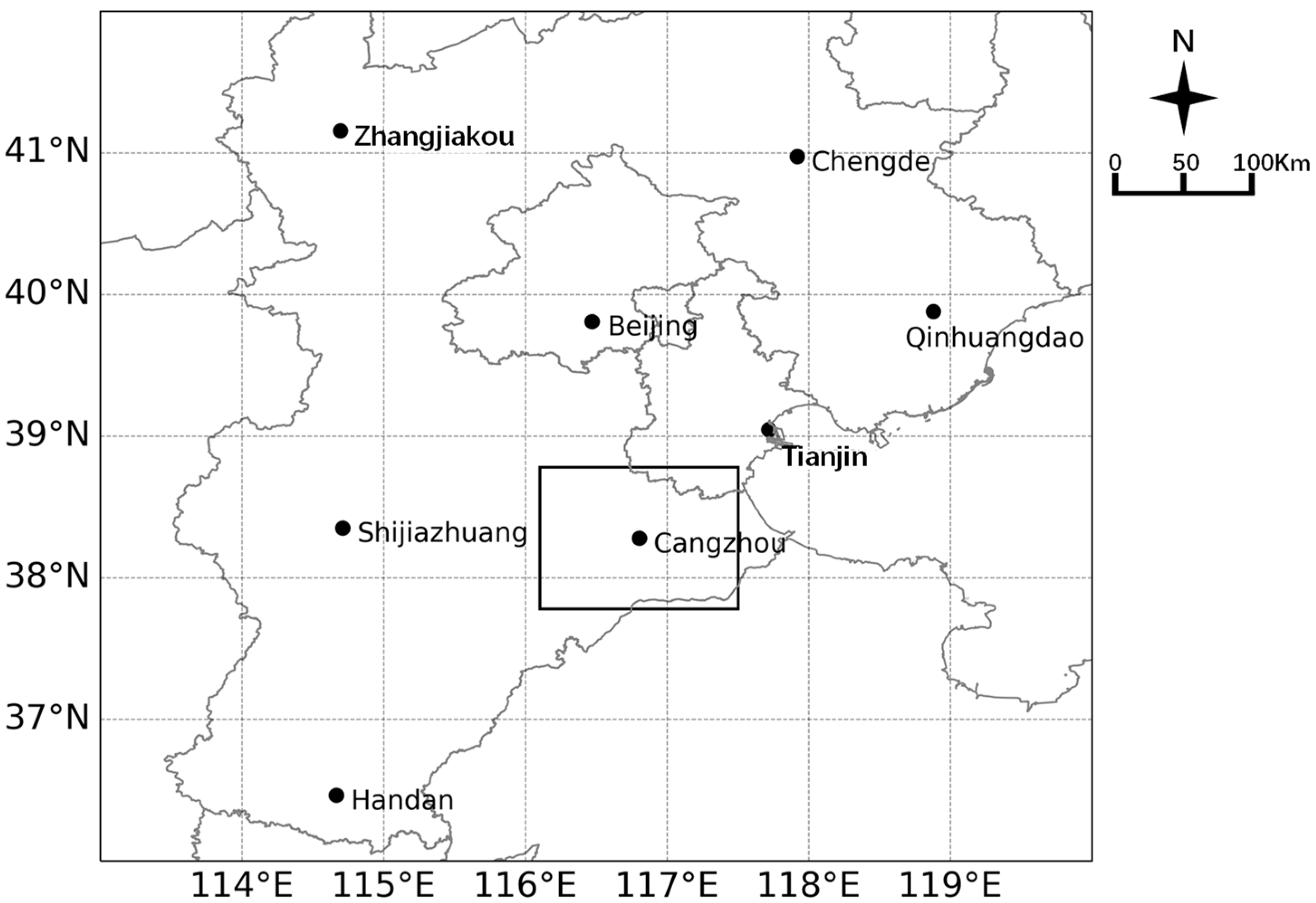
Benefiting from advancements in integrated meteorological observation systems, multi-source real-time data fusion analysis, and multiscale numerical forecasting models, regional meteorological centers in Beijing, Shanghai, Guangdong, and other areas in China have developed rapid update analysis and forecasting systems with a temporal resolution of 10–12 min and spatial resolution of 1 km. These systems provide initial fields capable of depicting real-time weather backgrounds with spatiotemporal resolutions comparable to radar observations. Therefore, effectively integrating such physical background information into deep learning-based radar echo extrapolation models—by fusing radar echoes with meteorological physical variables—can greatly enhance prediction accuracy.
To address the above challenges and leverage the emerging high-resolution weather background data, this study is motivated by two key objectives: (1) overcoming the blurriness and detail loss caused by conventional convolutional operations; (2) integrating physical constraints from meteorological background fields to improve the prediction of echo dynamics. The main contributions are as follows:
A fusion-encoder–decoder framework is designed for radar echo extrapolation, which couples deep convolutional generative adversarial networks (DCGAN) with time-series modeling to reduce echo blurriness and preserve fine-scale features.
Real-time weather background data (e.g., from RMAPS-NOW) are innovatively integrated into the deep learning model, providing physical constraints that mitigate error accumulation in long-term extrapolation.
The model assigns adaptive weights to long time sequences and strong echoes, significantly improving prediction accuracy for complex precipitation patterns, as validated by comprehensive experiments.

2. Data Sources and Data Preprocessing

The data used includes the North China radar composite reflectivity mosaic and the initial zero-field of the near-term numerical weather prediction subsystem (RMAPS-NOW) from the Beijing Urban Meteorological Research Institute’s next-generation rapid update multi-scale data analysis and forecasting system (RMAPS). Since this paper mainly discusses the feasibility of integrating weather background to improve radar echo extrapolation, and due to computational limitations, only the data within the range of 116.10–117.50°E and 37.77–38.77°N (indicated by the black box in Figure 1) is selected for training and modeling. This area is located in the southeastern part of Hebei Province, in the Heilonggang River Basin in the eastern Hebei Plain. It is situated in the eastern part of the Jizhong Plain, characterized by low and flat terrain with minimal undulation, sloping from southwest to northeast. The region experiences a warm temperate continental monsoon climate with distinct seasons and ample sunlight, and there is abundant and comprehensive surface meteorological data available for the area. The data covers the period from June to September, spanning from 2018 to 2022.

2.1. Radar Puzzle Data

The radar mosaic data were obtained from the “Tianqing” meteorological big data cloud platform, operated by the National Meteorological Information Center. The data have a spatial resolution of 0.01° and a temporal resolution of 6 min. Echo intensities below 0 dBZ were set to 0, while those exceeding 70 dBZ were capped at 70. The data were then normalized using Equation (1).
V n o r m = V i V min V max V min
In the equation, V n o r m denotes the normalized variable, V i represents the original data variable, and V m a x and V m i n are the predefined maximum and minimum values, respectively. After data selection, a total of 39,000 radar mosaic frames were obtained, of which 80% (31,200 frames) were used as the training set and 20% (7800 frames) as the test set. Each 180 min period, comprising 30 frames, was treated as a subset: the first 10 frames (corresponding to 60 min) were used as inputs, while the subsequent 20 frames (corresponding to 120 min) were used as labels for prediction.

2.2. RMAPS-NOW Data

The weather background data is sourced from the Beijing Urban Meteorological Research Institute’s next-generation rapid update multi-scale data analysis and forecasting system (RMAPS), specifically the near-term numerical weather prediction subsystem (RMAPS-NOW). This system integrates real-time data from over 2000 ground-based automatic stations with 5 min observations and results from the RMAPS-ST mesoscale numerical model. It provides real-time rapid analysis of regional high-resolution 3D atmospheric thermodynamic fields with a 10 min update cycle, as well as 0–2 h near-term numerical forecasts at 10 min intervals. The RMAPS coverage area is from 116.103°E to 117.503°E and from 37.770°N to 38.770°N, with a meridional resolution of 0.036° and a zonal resolution of 0.026°. To avoid limitations on echo extrapolation results due to model forecast accuracy, this study only uses the RMAPS-NOW initial zero-field data, which approximates actual conditions. The selected physical quantities are shown in Table 1.

2.3. Data Matching

Due to the differences in spatiotemporal resolution between RMAPS data and radar data, the radar mosaic data has a higher spatial resolution. To match the RMAPS data to the same spatial resolution as the radar, we use bilinear interpolation. Specifically, the weighted average of four RMAPS data points near the radar grid point is calculated, with closer data points assigned higher weights, in order to obtain the physical quantity values at the radar grid point location.
Considering that radar echoes typically lag behind weather background information, and to reduce interpolation errors, no interpolation is performed on the temporal axis between the radar data and RMAPS data. Instead, the 10 sets of RMAPS-NOW zero-field data for the preceding 100 min are directly matched with the 10 sets of radar mosaic data for the preceding 60 min.

3. Network Architecture Design and Model Training

3.1. ConvLSTM

Radar echoes are not only temporally interrelated, but more importantly, they also exhibit spatial correlation. Therefore, this study designs a network architecture that incorporates weather backgrounds based on the ConvLSTM framework, which has good capabilities for extracting temporal and spatial features. ConvLSTM is a neural network model that combines Convolutional Neural Networks (CNN) and LSTM. LSTM, a variant of Recurrent Neural Network (RNN), demonstrates strong long-term dependency modeling capabilities when processing sequential data. It selectively forgets and updates information through gating units, enabling better capture of long-term dependencies in time series. ConvLSTM, an extension of LSTM, introduces convolutional operations, allowing it to process both spatial and temporal information simultaneously (Equation (2)).
i t = σ ( W f [ H t 1 , X t ] + b i ) f t = σ ( W f [ H t 1 , X t ] + b f ) O t = σ ( W o [ H t 1 , X t ] + b o ) C t ~ = tanh ( W c [ H t 1 , X t ] + b c ) C t = f t C t 1 + i t C ~ t H t = O t tanh ( C t )
In the equation, ∗ denotes the convolution operation, i t is the input gate at time step t, X t is the input data at time step t (typically a convolved feature map); f t is the forget gate at time step t, with parameters similar to those of the input gate; O t is the output gate at time step t; C t and C t 1 are the cell states at time steps t and t − 1, respectively; C t ~ is the fused information at time step t; H t and H t 1 are the hidden states at time steps t and t − 1, respectively; W represents the corresponding convolutional kernel parameters; b is the bias term; σ is the sigmoid activation function, which avoids gradient vanishing and offers good convergence and computational efficiency; tanh is the hyperbolic tangent activation function, whose nonlinear transformation characteristics endow the network with the ability to learn complex relationships.

3.2. Radar Cell Encoding

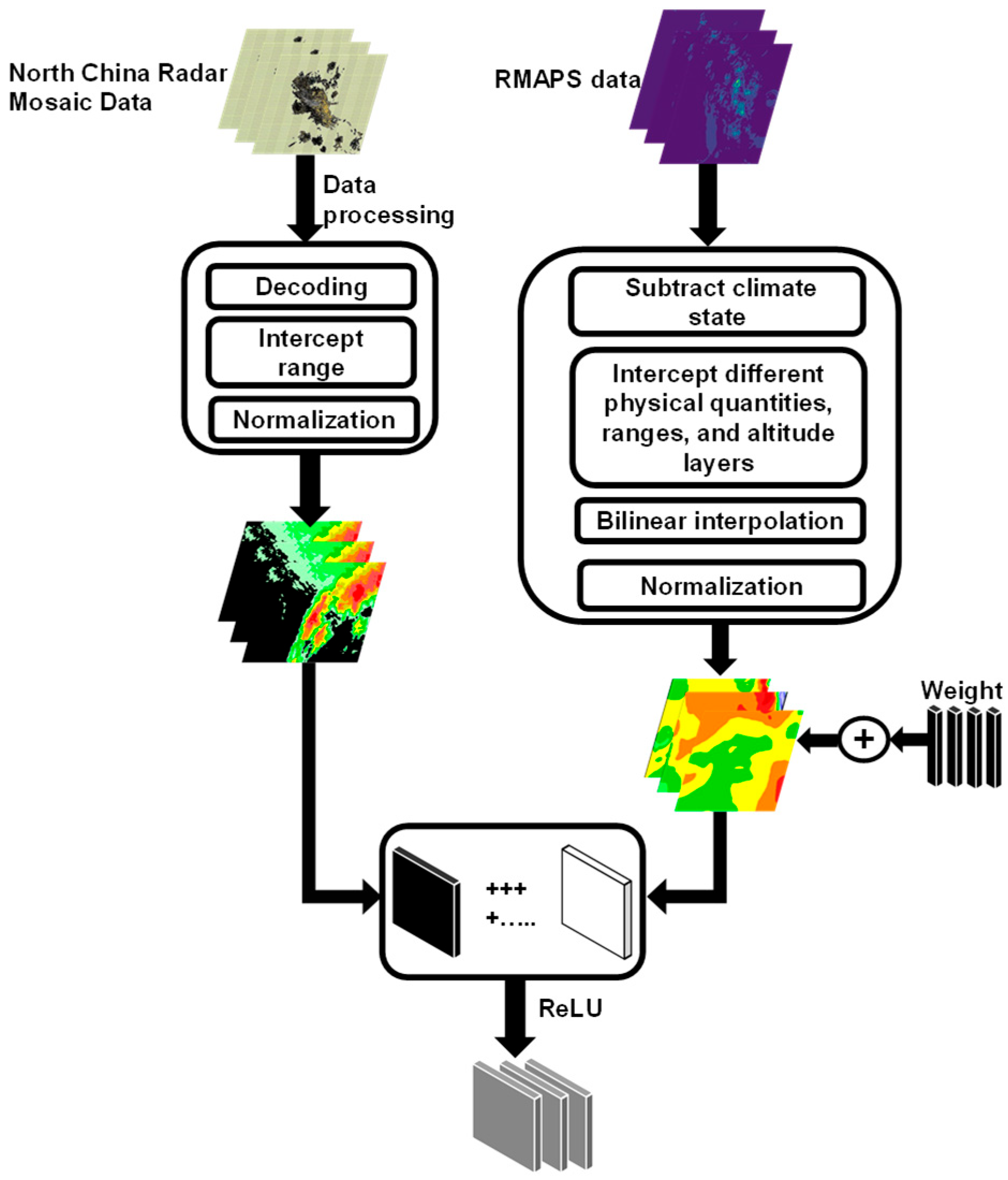
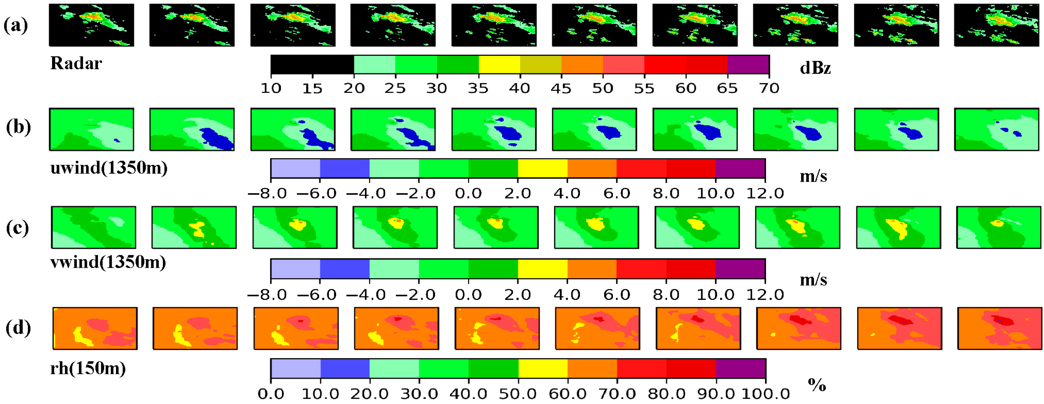
A radar cell was constructed by multiplying a given physical variable (e.g., relative humidity, u-wind, or v-wind) by an initially assigned weight and stacking it with the corresponding radar echo intensity matrix, thereby integrating information from a single physical variable (Figure 2). The weight is automatically optimized during the model training process. The formulation of the radar cell is given in Equation (3):
R a d a r c e l l _ o u t = R e L U ( w r [ 1 ] · x 1 + w r [ 2 ] · x 2 + w r [ 3 ] · x 3 + + w r [ i ] · x i + b r )
In this equation, R a d a r c e l l _ o u t represents the matrix resulting from the fusion of weather background information and radar echoes, reflecting the influence of external meteorological factors on the radar data. w _ r i denotes the learnable weight parameters, x i represents the input physical variables, and b r is a trainable bias term introduced to enhance the model’s adaptability. The ReLU activation function is applied to ensure non-negative outputs, thereby enforcing that the fusion process only introduces positive corrections to the data without introducing negative interference.
For each physical variable, 1 to 3 grid fields at different vertical levels were selected (see Table 1 for details). A scaling parameter (Scale) was used to adjust the relative weights of different physical variables. These variables were then fused with the corresponding radar echo sequences to generate multiple radar cells, each incorporating distinct background meteorological information. After applying weighting and normalization to each radar cell, they were further encoded into ConvLSTM cells based on the ConvLSTM architecture, and used as the input sequence for the ConvLSTM network.
Batch normalization was applied to both the previous hidden state H t 1 and the input ConvLSTM cell to enhance the model’s generalization ability and to mitigate issues such as gradient vanishing or explosion, thereby improving training efficiency and model performance. The ConvLSTM cell served as the input gate, performing forward propagation using convolutional operations, allowing spatially dependent information to flow across time steps through the computation and activation of various gates and cell states.
Finally, a Squeeze-and-Excitation Layer (SELayer) was introduced to return the attention-weighted hidden state H t and the updated cell state C t . The self-attention mechanism applied to the hidden state enhances the model’s ability to learn important channel features, thereby improving its representational capacity.

3.3. MR-DCGAN Network Architecture

In traditional radar echo extrapolation, the quality of predicted echoes significantly deteriorates as the forecast lead time increases, leading to issues such as difficulties in echo tracking, increased uncertainty in identification, and greater complexity in data processing. Moreover, deep learning-based echo extrapolation models typically rely on pixel-wise loss functions, which often result in image distortion during prediction. Deep Convolutional Generative Adversarial Networks (DCGANs) are capable of effectively capturing the spatial features of radar echo images and reconstructing them in a reverse manner, thereby alleviating the blurring problem commonly observed in extrapolated outputs.
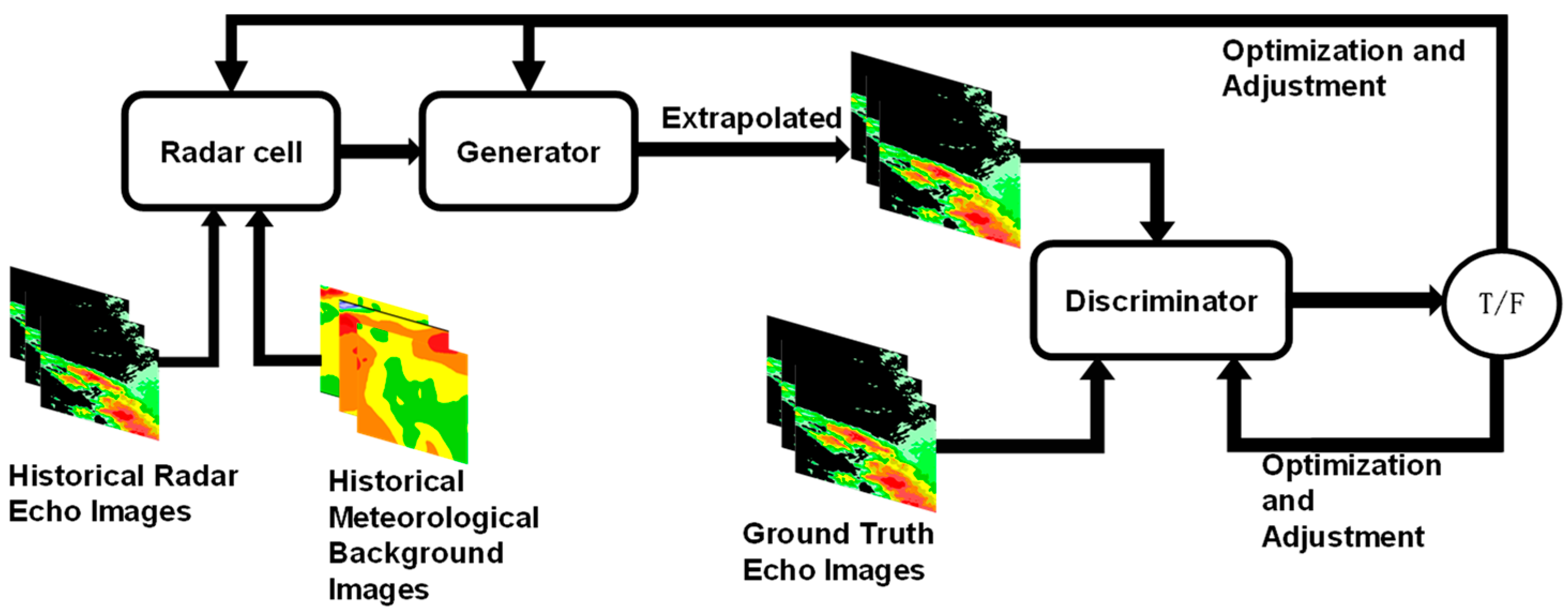
A generative adversarial network primarily consists of a generator and a discriminator The MR-DCGAN network architecture proposed in this study (Figure 3) builds upon the MR-ConvLSTM model (Figure 4) developed by Wang Shanhao et al. [
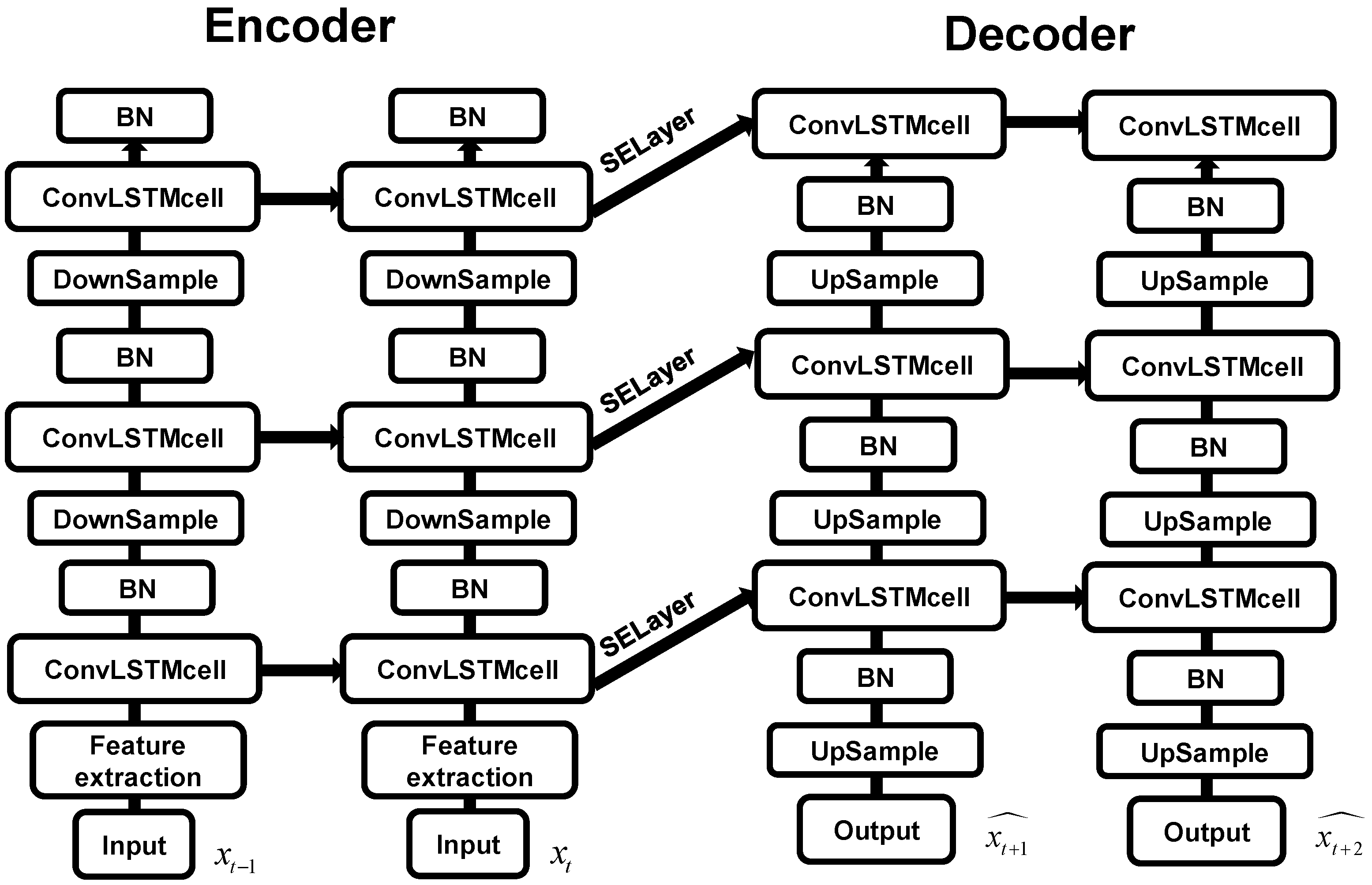
43]. In this architecture, we employed an Encoder–Decoder framework to predict spatio-temporal sequences. Building upon this structure, we integrated ConvLSTM cells constructed from multiple radar units of RMAPS-NOW into the encoder–decoder architecture, further developing the MR-ConvLSTM network architecture.
The encoder consists of three downsampling layers and three ConvLSTM cell layers. It transforms the input hidden states into a fixed-length vector encapsulating information from the input sequence. The hidden state from the final encoding step initializes the decoder’s hidden states. After each encoding step, the input to the ConvLSTM cells is downsampled via convolution to extract critical spatial features, enabling the ConvLSTM cells to better learn radar echo characteristics integrated with weather background information. Batch normalization is applied after each ConvLSTM cell layer to enhance model generalization. The Leaky-ReLU activation function is used to mitigate the vanishing gradient issue in the negative region.
The decoder prediction module comprises three upsampling layers and three ConvLSTM cell layers. At the input of each ConvLSTM cell layer, an SELayer (Squeeze-and-Excitation Layer) is introduced to strengthen skip connections between the encoder and decoder. The decoder processes the context vector from the encoder, using the last frame of the encoded input as its initial input. Through an attention mechanism, it learns features to generate the target sequence, achieving spatio-temporal prediction. After each decoding step, deconvolution (upsampling) is performed to expand the feature maps, allowing the ConvLSTM cells to learn upsampled features and reconstruct future radar echo sequences. Batch normalization is also applied after each ConvLSTM cell layer.
Finally, the output sequences are stacked and dimension-transformed. A CNN is applied at the decoder’s final stage to further adjust feature dimensions and enhance representational capacity, generating the predicted output. This process iterates to produce the final radar echo extrapolation sequence.
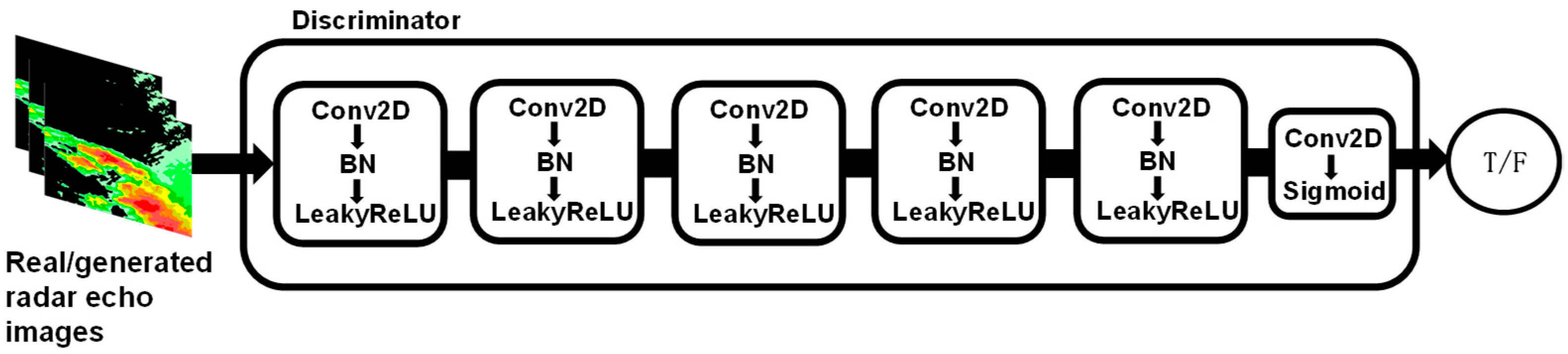
The discriminator is used to assess the authenticity of the input images. The network structure of the discriminator (Figure 5) consists of six layers. The first to fifth layers are composed of convolutional blocks, while the sixth layer includes a Conv2D convolutional layer followed by a Sigmoid activation function layer. Each convolutional block consists of a Conv2D convolutional layer, a BatchNorm layer for batch normalization, and a LeakyReLU activation function. This structure effectively extracts local features from the echo images and continuously optimizes the generator during training, ensuring that the generated echo predictions are more consistent with the ground truth. Additionally, it enhances the accuracy and stability of long-term extrapolation.
In this study, an alternating optimization strategy will be employed for model training to achieve a dynamic game relationship between the generator and the discriminator, thereby improving the quality and authenticity of the generated results. The training process consists of the following two main stages:
Discriminator Training Stage: During the discriminator training, the generator network and the module parameters for integrating weather background variables are kept fixed. The generator network, based on its own structure and parameters, generates simulated radar echo data from specific random noise or latent features. The module that integrates weather background variables takes into account various meteorological factors and generates data by fusing weather background physical variables with radar echo data through radar cells. This fusion ensures that the generated data better aligns with actual meteorological conditions. The real radar echo data and the simulated data generated by the generator are then input into the discriminator network. The discriminator network analyzes the input data features and determines whether the data is real radar echo data or simulated data. It uses an optimization algorithm to adjust its parameters to minimize the discrimination error. After multiple iterations of training, the discriminator’s parameters are continuously optimized, and its ability to discriminate improves, ultimately enabling accurate identification of real radar echo images, thereby providing feedback for generator training.
Generator Training Stage: During the generator training, the parameters of the discriminator network are fixed. The main task of the generator network is to generate radar echo image data based on the input random noise and latent features. The radar cells are responsible for fusing weather background physical variables with the radar echo data during the generation process, thereby enhancing the authenticity and plausibility of the output data. During training, the generator continuously generates new radar echo image data and inputs these data into the discriminator with fixed parameters for evaluation. The discriminator provides feedback on the authenticity of the generated data based on its judgment criteria. The generator then uses this feedback and optimization algorithms to adjust its parameters, allowing it to generate radar echo images that are as close as possible to real radar echoes, thus improving the spatiotemporal consistency and structural integrity of the generated samples.
Through alternating training of the generator and discriminator, the discriminator continuously improves its ability to distinguish between real and generated data, while the generator progressively optimizes itself during the adversarial process, causing the generated radar echo data to approach the real echo distribution. Ultimately, this process leads the model to reach a Nash Equilibrium, where the discriminator can no longer effectively distinguish between real and generated data, ensuring that the extrapolated results maintain consistency with real radar echoes in terms of data distribution, thereby improving the accuracy of long-term sequence predictions.

3.4. Custom Loss Function

In the Generative Adversarial Network (GAN), the discriminator is a logistic regression model, and thus the loss function is defined as binary cross-entropy loss, as shown in Equation (4):
B C E L oss i = 1 N i N [ y i log ( p i ) + ( 1 y i ) log ( 1 p i ) ]
where N is the number of samples, y i is the label value, p i is the predicted probability, and l t is the spatial dimension weight loss function (Equation (7)). For the discriminator, when i = 0, real samples are used to train the discriminator, with y i being the real value; when i = 1, generated samples are used to train the discriminator, with y i being the fake value; and when i = 2, generated samples are used to train the generator, with y i being the real value. The loss functions for the discriminator and generator used in this chapter are shown in Equations (5) and (6), respectively:
D l o s s = B C E L o s s 0 + B C E L o s s 1
G l o s s = B C E L o s s 2 + l ( t )
l ( t ) = i = 0 H 1 j = 0 W 1 w i , j , t | y p r e d , i , j , t y g d , i , j , t | + i = 0 H 1 j = 0 W 1 w i , j , t ( y p r e d , i , j , t y g d , i , j , t ) 2
To further improve the extrapolation performance of long time series, this chapter independently trains the model for each forecast time step based on different physical quantity inputs, thereby constructing 20 sub-models for extrapolation at different time steps. This time-step-specific training strategy allows the model to optimize at each time step, enabling each sub-model to more accurately learn the specific echo features within its corresponding time step. This approach reduces the mutual interference between different time steps, lowers model complexity, enhances the local generalization ability, and simultaneously improves the model’s adaptability to echo evolution across different time scales.
Although this method has higher computational requirements, fine-tuning parameters and optimization strategies can significantly improve overall prediction accuracy, especially in terms of maintaining strong echoes and restoring spatial details. Finally, through extensive experiments and tests, the optimal time-step weight matrix was determined, as shown in Table 2. The vertical dimension of this matrix represents the forecast time steps, while the horizontal dimension corresponds to different echo intensity ranges. This matrix is used to adjust the weights of each part in the loss function, further enhancing the extrapolation model’s prediction stability and accuracy across different echo intensity ranges.

3.5. Model Training

The focus of this study is to validate the performance of the radar echo extrapolation model, which incorporates weather background information, when integrating DCGAN and time-sequencing modeling methods. Therefore, in the comparative experiments, Unet and ConvLSTM models, which do not include weather background information, were selected as benchmark models to assess the improvements in extrapolation results brought about by the optimizations presented in this chapter. Considering computational constraints, no further algorithms were included for comparison to avoid introducing too many variables, which could impact the interpretability of the experimental results.
The experiments were based on MR-DCGAN, ConvLSTM, and Unet structures without the inclusion of physical quantities. Five different input encoding schemes were designed, and except for the ConvLSTM and Unet models that did not include physical quantities, the other architectures each trained 20 time-sequencing models. The experimental extrapolation models are shown in Table 3 below:
All experiments were conducted with the same hyperparameter configuration to ensure the comparability of the results. The initial learning rate was set to 0.0001, the batch size was 5, and the maximum number of iterations was 400. To prevent overfitting, an early stopping mechanism was implemented. If the loss function was not optimized over 30 consecutive epochs, the training process was prematurely terminated, and the best model parameters were saved. The Adam optimizer was used during the optimization process to further improve the model’s convergence and stability.

3.6. Evaluation Indicators

A binary classification model based on predefined thresholds, commonly used in meteorological operations, is employed to assess the model’s performance. The reflectivity thresholds are selected as 20, 30, and 35 dBZ, with a forecast time interval of 6 min. The model’s ability to correctly predict is evaluated using the Probability of Detection (POD), the False Alarm Rate (FAR) is used to assess erroneous predictions of events that did not occur, and the Critical Success Index (CSI) is used to measure the overall performance of the model (Equation (8)).
In Equation (8), each value is calculated from the confusion matrix (Table 4). The True Positives (TP) represent the points where both the predicted value and the actual value exceed the threshold, False Negatives (FN) represent the points where the predicted value exceeds the threshold but the actual value does not, False Positives (FP) represent the points where the predicted value is below the threshold but the actual value exceeds the threshold, and True Negatives (TN) represent the points where both the predicted and actual values are below the threshold.
By comparing the predicted values with the observed values for each grid point, the classification for each point is determined, and the evaluation metrics are then calculated. The methods for calculating POD, FAR, and CSI are shown in Equation (8). Higher values of POD and CSI indicate more accurate predictions, while a lower FAR value indicates better prediction accuracy.
P O D = T P T P + F N F A R = F P T P + F P C S I = T P T P + F N + F P
To more comprehensively evaluate the model, the Structural Similarity (SSIM) index was further introduced to assess the visual quality and structural preservation capabilities between predicted radar echo images and actual observational data. SSIM integrates luminance, contrast, and structural information of images. By calculating the similarity between predicted and real images across these features, it quantifies the model’s ability to retain fine-grained echo details. The SSIM formula is presented in Equation (9):
S S I M ( x , y ) = ( 2 μ x μ y + C 1 ) ( 2 σ x y + C 2 ) ( μ x 2 + μ y 2 + C 1 ) ( σ x 2 + σ y 2 + C 2 )
where x and y denote the real radar echo image and predicted echo image, respectively; μ X and μ y represent the pixel-wise means of x and y; σ x 2 and σ y 2 are their pixel variances; σ x y is the pixel covariance between them; constants C1 and C2 are primarily used to enhance numerical stability.

4. Model Evaluation

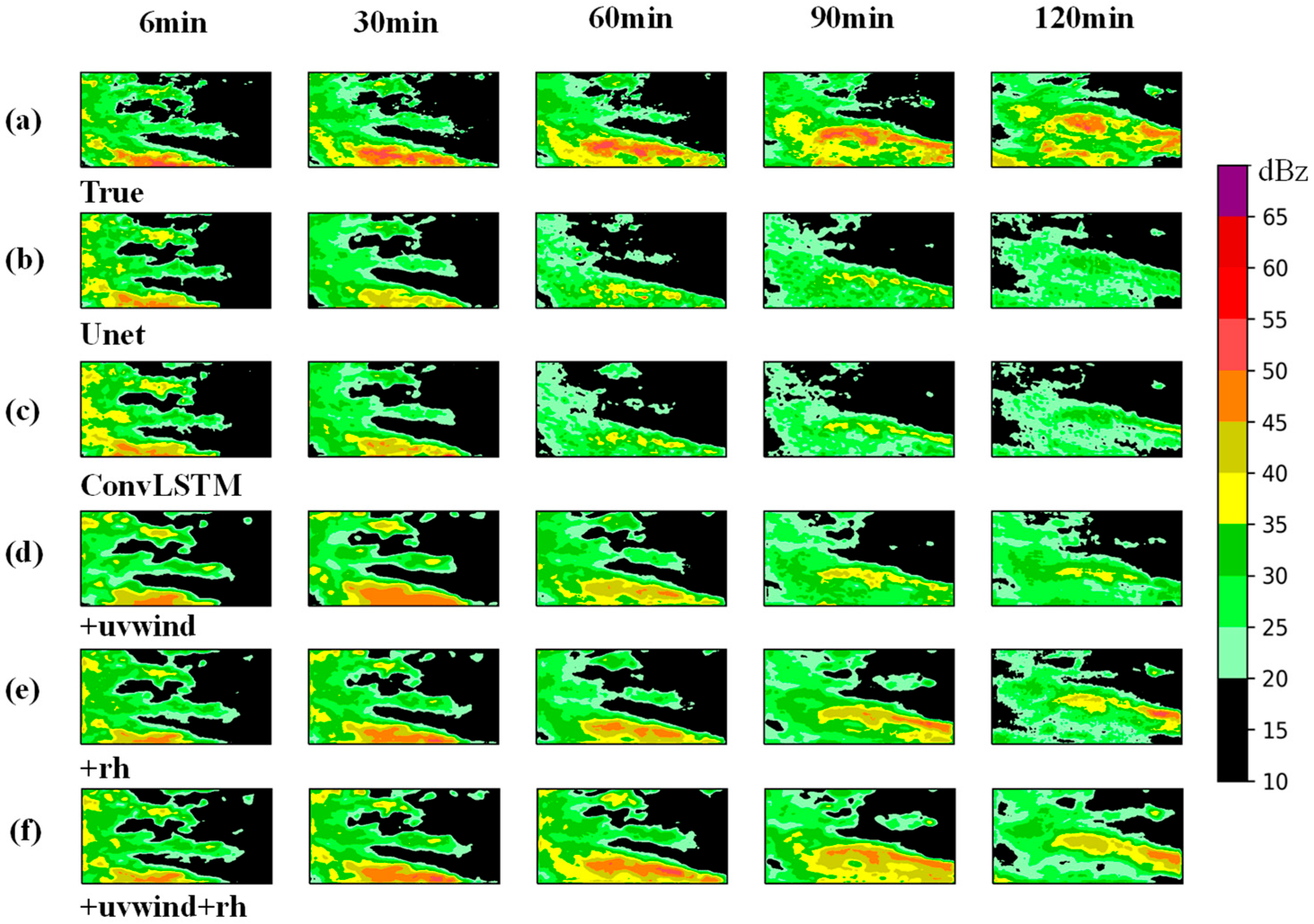
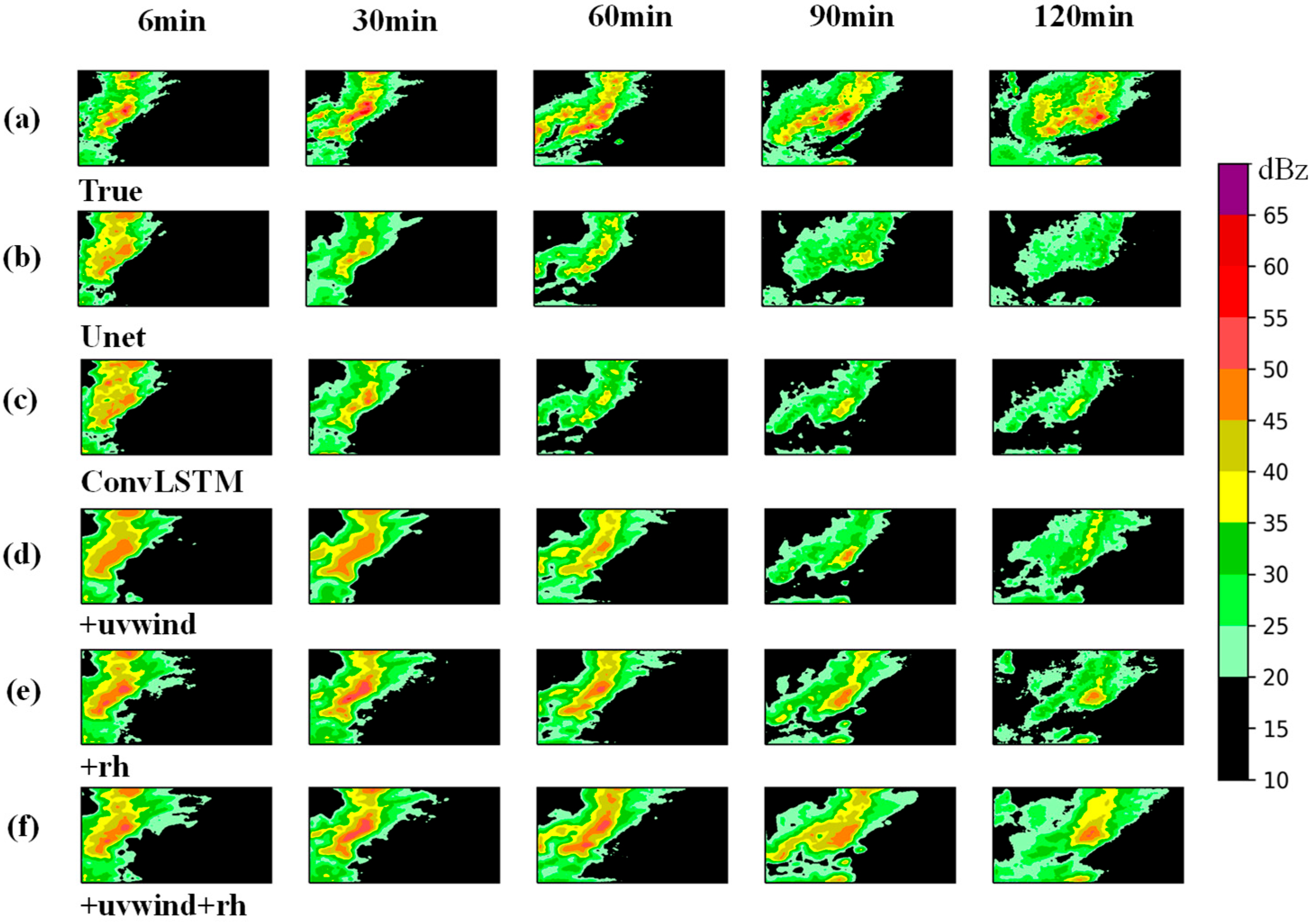
In this study, a total of 20 radar echo extrapolation models were trained based on three network architectures—Unet, ConvLSTM, and MR-DCGAN—and five different input encoding schemes. These models were then evaluated using a testing dataset to perform radar echo extrapolation and assess model performance.
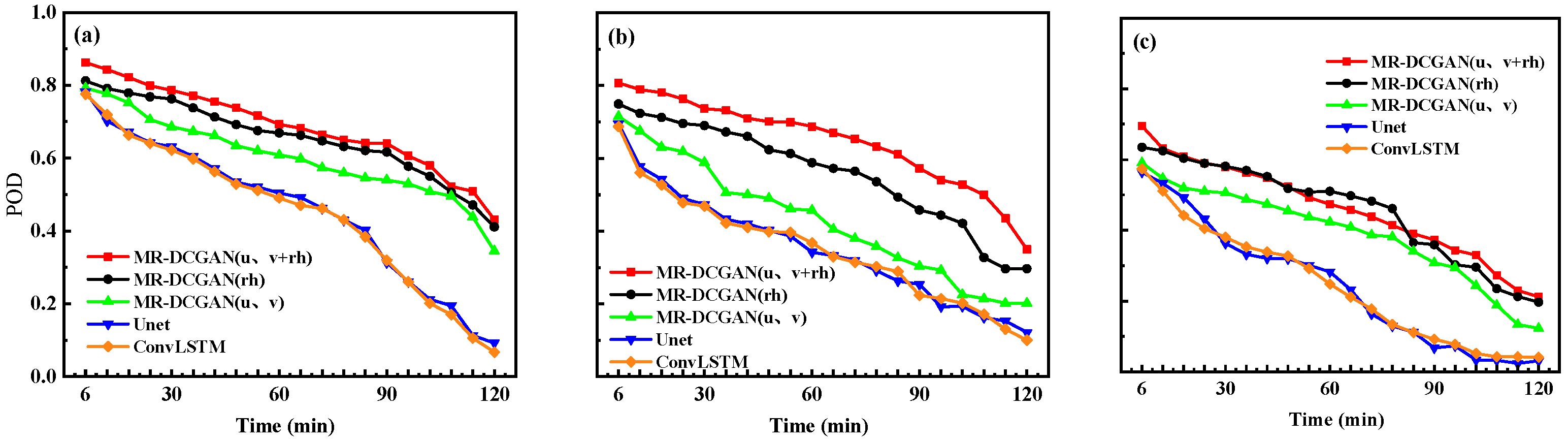
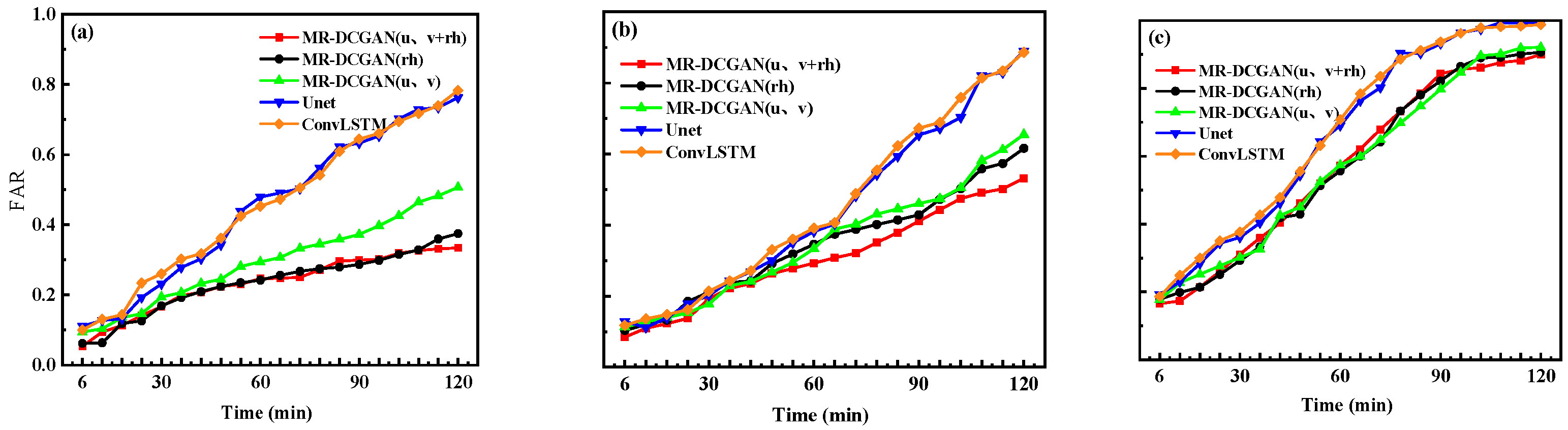
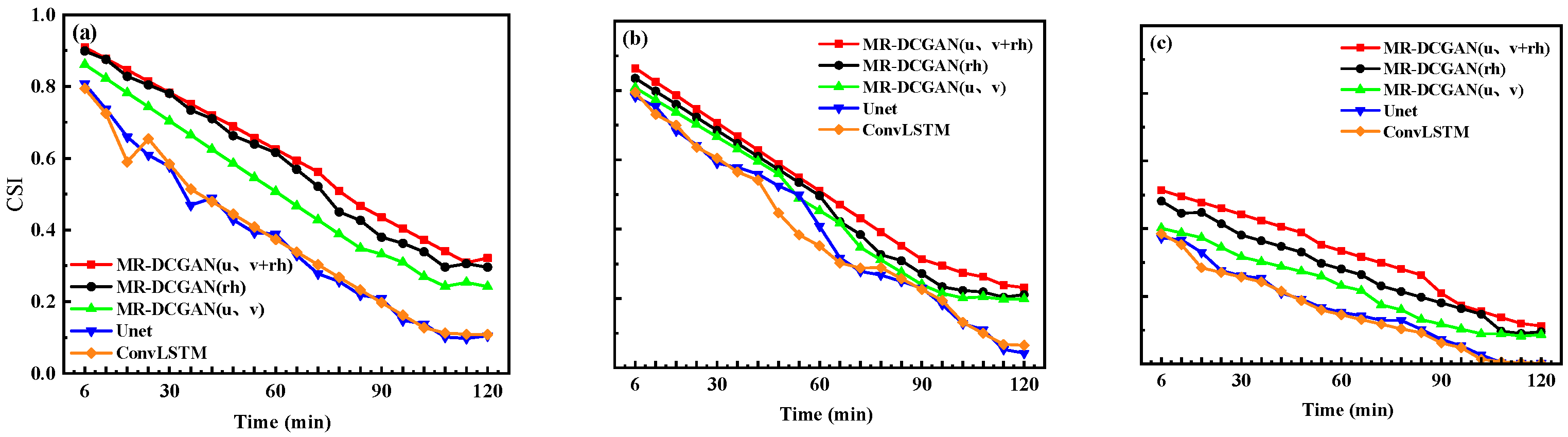
To comprehensively evaluate the extrapolation performance, radar echo intensity thresholds of 20, 30, and 35 dBZ were selected. For each threshold, the Probability of Detection (POD), False Alarm Rate (FAR), and Critical Success Index (CSI) were calculated for the different models on the test set.
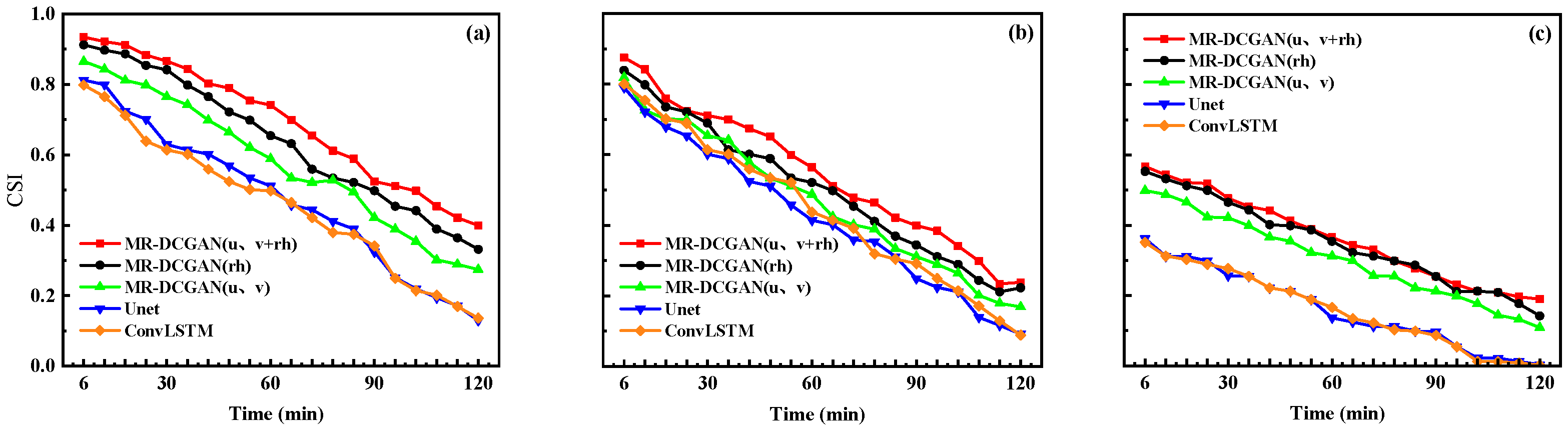
 Figure 6, Figure 7 and Figure 8 illustrate the extrapolation performance metrics over successive 6 min intervals for models trained with different input encodings based on the MR-DCGAN, Unet, and ConvLSTM architectures (without incorporating physical variables). Table 5 further presents the average values of POD, FAR, and CSI for the 120 min extrapolation horizon.
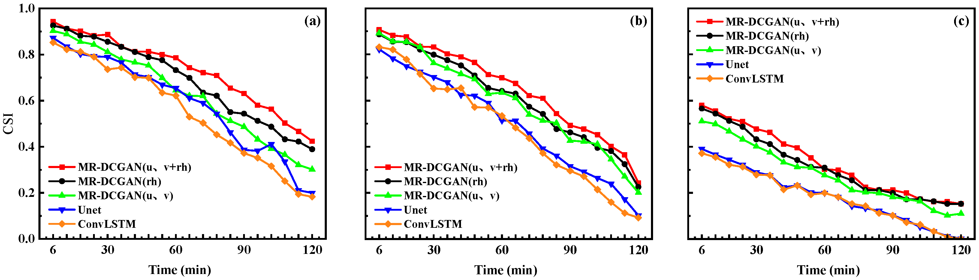
As shown in Figure 6, Figure 7 and Figure 8, and 
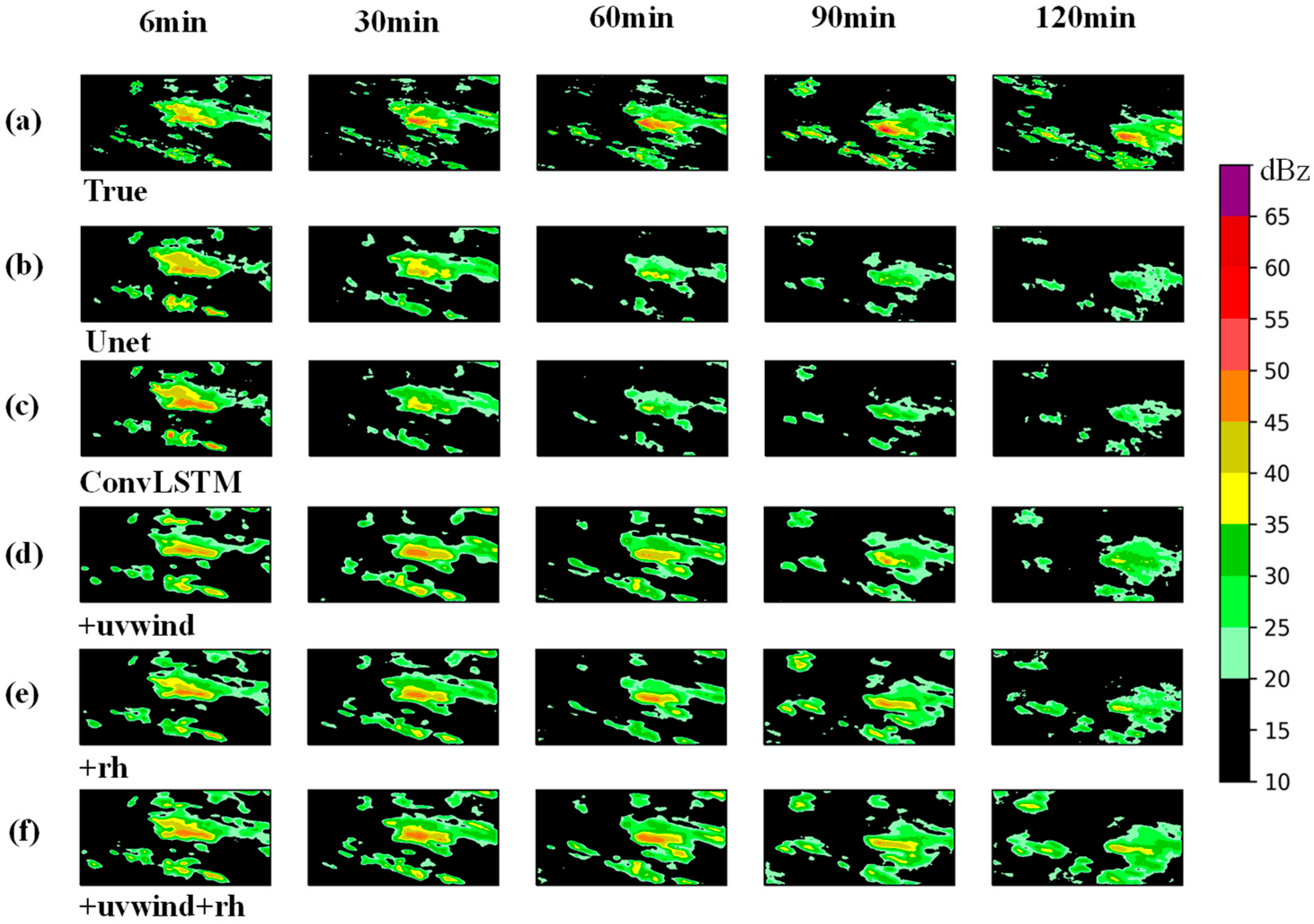
Table 5, with increasing radar echo intensity thresholds, both POD and CSI exhibit a declining trend, while FAR increases. In comparison to the Unet and ConvLSTM models, the extrapolation models trained with MR-DCGAN demonstrate significant improvements in CSI and POD across all thresholds, along with a marked reduction in FAR. Specifically, the CSI values of the MR-DCGAN model increase by 18.59%, 8.76%, and 11.28% over the Unet and ConvLSTM models at thresholds of 20 dBZ, 30 dBZ, and 35 dBZ, respectively. The corresponding improvements in POD are 19.46%, 19.21%, and 19.18%, while FAR is reduced by 19.85%, 11.48%, and 9.88%, respectively. These results indicate that incorporating physical variables can effectively enhance the accuracy of radar echo extrapolation and improve the model’s predictive capability under various echo intensity levels.
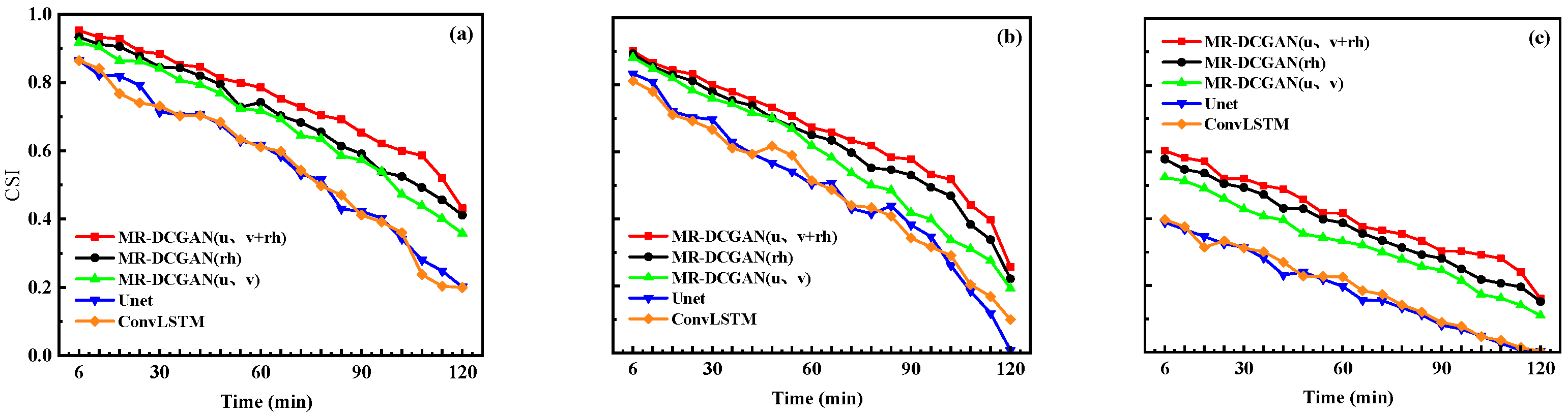
According to the results summarized in Table 4, the MR-DCGAN model incorporating three physical variables (u, v wind components, and relative humidity) significantly outperforms the models without physical variable integration across different radar reflectivity thresholds. Specifically, the Critical Success Index (CSI) and Probability of Detection (POD) show average improvements of 16.75% and 24.75%, respectively, while the False Alarm Ratio (FAR) decreases by an average of 15.36%.
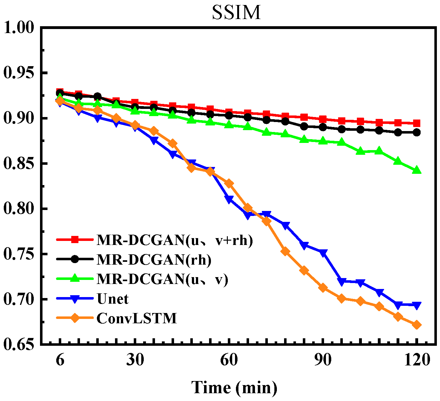
To further evaluate the visual quality of predicted images, this study introduced the SSIM metric for analysis. The variation curves of SSIM values over 20 time steps are presented in Figure 9. As shown in the figure, the SSIM values of all models gradually decline over time. Notably, the MR-DCGAN model proposed in this research exhibits a slower and more stable decay throughout the extrapolation process, with its superiority becoming particularly pronounced in the latter half of the prediction horizon. Among all configurations, the model integrating u/v and rh physical variables demonstrates the optimal performance.
These findings indicate that integrating complex physical variables can effectively enhance the model’s extrapolation capability for varying reflectivity intensities, leading to predictions that are more physically consistent and spatiotemporally coherent.

5. Model Application

The extrapolation results on the test dataset demonstrate that the model trained based on the MR-DCGAN architecture with incorporated meteorological background variables exhibits a significant advantage in radar echo extrapolation performance compared to the ConvLSTM and U-Net models without such background information. To further illustrate the improvements achieved by the proposed model, this section presents an analysis of three representative cases randomly selected from the test dataset.

5.1. Example 1

From 11:30 to 13:30 BJT on 25 June 2020, under the influence of an upper-level cold vortex, strong convective weather—including short-duration heavy rainfall, hail, and thunderstorm-induced gales—was observed in Cangzhou, Baoding, and Langfang, Hebei Province. Figure 10 shows the radar echoes of the first 10 time series in the input and the physical quantity data. Due to the limited length of the article, the input physical quantities for the subsequent individual cases will not be provided. The observed and extrapolated radar echo results at 6, 30, 60, 90, and 120 min are shown in Figure 11.
At 6 and 30 min, the models incorporating meteorological variables showed similar performance in predicting strong echoes, whereas models without physical variables significantly underestimated strong echoes. After 60 min, the predictive performance of all models declined. Notably, models without physical variables failed to capture echoes above 35 dBZ at 90 and 120 min. In contrast, models incorporating relative humidity (rh) and u/v wind components retained the ability to predict strong central echoes at 90 and 120 min, demonstrating superior capability in modeling echo dependencies over medium-to-long time horizons, as well as enhanced robustness in the temporal dimension.
To further evaluate the extrapolation accuracy of each model for this specific case, the variations in the Critical Success Index (CSI) over 6 min intervals under reflectivity thresholds of 20, 30, and 35 dBZ were analyzed and compared, as shown in Figure 12. The MR-DCGAN (u, v + rh) model demonstrates average CSI improvements of 21.6%, 12.3%, and 21.1% over the Unet model and 23.2%, 10.4%, and 20.1% over the ConvLSTM model at the 20, 30, and 35 dBZ thresholds, respectively. Among all models, the MR-DCGAN (u, v + rh) model shows the slowest decline in CSI, indicating its superior ability to maintain echo structure characteristics during medium- to long-term extrapolation and delivering enhanced prediction accuracy.

5.2. Example 2

From 03:00 to 05:00 on 12 August 2020, the eastern region of Hebei Province experienced a heavy rainfall event under the combined influence of the subtropical high, an upper-level trough, and a shear line. Figure 13 shows the actual observations and extrapolated predictions from different models at various time steps. Overall, the predictive accuracy of all models for strong echoes declined over time, especially after 90 min, with a noticeable deterioration in the integrity of the echo structure.
Among them, the models that did not incorporate physical variables showed a significant weakening of echo intensity at the 90–120 min forecast time, with little ability to effectively capture strong echoes above 45 dBZ, exhibiting a strong attenuation trend. In contrast, the three models that included physical variables were able to maintain the overall structure of strong echoes relatively well at the 90–120 min forecast time. The MR-DCGAN (u, v + rh) model demonstrated a certain ability to predict strong echoes above 45 dBZ, with echo distribution being more continuous compared to the models without physical variables. This model was able to more fully predict the spatial structure and intensity characteristics of the heavy precipitation region.
The variation curves of the CSI evaluation metrics for the extrapolation results of each model at 20, 30, and 35 dBZ reflectivity conditions, with a 6 min interval over 20 time steps, are shown in Figure 14. The CSI values of the MR-DCGAN (u, v + rh) model are, on average, 14.2%, 15.3%, and 14.6% higher than those of the models without physical variables (Unet, ConvLSTM), and 17.9%, 17.2%, and 15.1% higher, respectively. It can be concluded that models incorporating physical variables yield higher CSI values than those without. Among them, the MR-DCGAN model with rh, u, and v as input variables performs the best, with its CSI values consistently higher than those of models without physical variables. Even under higher reflectivity thresholds, the model still exhibits good prediction performance.

5.3. Example 3

From 15:00 to 17:00 on 17 July 2021, under the influence of the shear line on the edge of the subtropical high, heavy, to very heavy rainfall occurred in Beijing, Shijiazhuang, Baoding, and Xingtai. The real-time and extrapolated results at 6, 30, 60, 90, and 120 min are shown in Figure 15.
Overall, the extrapolation results are similar to those in Cases 1 and 2. The model that did not incorporate physical quantities showed a more significant decline in predicting the central strong echoes after 60 min. The models that introduced either relative humidity (rh) or u/v winds showed a smaller prediction range for the central echoes at 90 and 120 min. However, the model that incorporated both rh and u/v winds produced predictions that were much closer to the real situation, with a larger predicted range for strong echoes.
Under the conditions of 20, 30, and 35 dBZ reflectivity values, the variations in the CSI evaluation metrics for different models at 6 min intervals are shown in Figure 16. From the overall trend of the line graphs, the MR-DCGAN (u, v + rh) model continues to maintain a leading performance. Its performance in case three testing is, on average, 18.3%, 17.1%, and 19.8% higher than the models without physical variables (Unet, ConvLSTM), and 18.8%, 16.6%, and 21.1% higher, respectively.
The combination of weather background parameter data and radar echo data can be used for the implementation of radar echo extrapolation in the 0–2 h range. Through both qualitative and quantitative analysis of three different cases, the visualization results indicate that the extrapolation model incorporating physical quantities performs better than the model without physical quantities for radar echo extrapolation. Moreover, the more complex the physical quantities introduced into the radar extrapolation model, the better the extrapolation performance. The Generative Adversarial Network (GAN) also improves the clarity of the predicted images, demonstrating a certain level of extrapolation capability across different radar echo threshold ranges.

6. Comparative Experiment

To better demonstrate the advantages of the MR-DCGAN architecture in radar echo extrapolation, a comparative experiment was conducted by selecting the MR-ConvLSTM [43] architecture for comparison with the proposed architecture in this paper. The comparative model adopted was the MR-ConvLSTM (u, v + rh) model with the best test performance, while the MR-DCGAN (u, v + rh) model with the optimal performance in this study was also chosen for intuitive result presentation. The test dataset was the same as the echo extrapolation model’s test data for the Cangzhou region used in this paper. To eliminate the influence of different data dimensions, all selected data were uniformly normalized, which effectively improved the comparability of the data and the stability of model training, ensuring the scientificity and rigor of testing the generalization ability of the MR-DCGAN (u, v + rh) model.
In the comparative experiment, POD (Probability of Detection), FAR (False Alarm Rate), CSI (Critical Success Index), and SSIM (Structural Similarity Index) were selected as evaluation metrics. These metrics not only enable quantitative evaluation of the models’ precipitation prediction capabilities but also comprehensively reflect the similarity between the predicted images and the real echo images. By using these four numerical indicators, the extrapolation performance of the models can be tested more objectively.
According to Table 6, the CSI of the MR-DCGAN (u, v + rh) model was on average 4.08%, 3.79%, and 3.15% higher than that of the MR-ConvLSTM (u, v + rh) model under the reflectivity thresholds of 20 dBZ, 30 dBZ, and 35 dBZ, respectively. The POD increased by 2.24%, 1.72%, and 2.99%, while the FAR decreased by 2.39%, 1.47%, and 4.19%. These experimental data demonstrate that the MR-DCGAN (u, v + rh) model outperforms the MR-ConvLSTM (u, v + rh) model in radar echo extrapolation tasks under the same test dataset. It can improve the prediction rate while reducing the false alarm rate, further indicating that the MR-DCGAN (u, v + rh) model has better extrapolation performance.
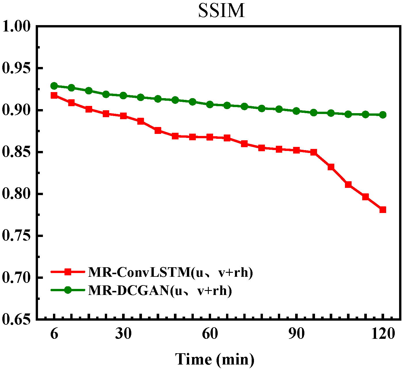
Figure 17 shows the variation trend of the Structural Similarity Index (SSIM) for the two models in radar echo prediction tasks. It can be seen that the decay process of the SSIM index is relatively smooth for both the MR-DCGAN (u, v + rh) and MR-ConvLSTM (u, v + rh) models, indicating that both models can maintain a certain structural similarity during prediction. In the initial stage of prediction, the echo images generated by the MR-DCGAN (u, v + rh) model exhibit higher similarity to the real echoes, suggesting that this model has better structural fidelity in short-term prediction.
In summary, the MR-DCGAN (u, v + rh) model exhibits superior performance in short-term prediction and demonstrates strong generalization capabilities across various time intervals in extrapolation tasks. It can adapt more stably to diverse meteorological conditions, thereby enhancing the reliability and applicability of radar echo prediction.

7. Discussion

In recent years, deep learning-based radar echo extrapolation has become the mainstream extrapolation algorithm. However, most of these extrapolation network architectures are based on convolutional discriminative networks, which take radar echo images as input and transform pseudo-color echo intensities, ranging from −5 to 70 dBZ with a resolution of 5 dB, into grayscale images with values from 0 to 255. This process inevitably loses many echo details. As the extrapolation time increases, the convolutional smoothing effect causes the image to become increasingly blurry. Furthermore, the evolution of radar echoes is actually the result of interactions between weather background processes. With advancements in technology, a large volume of detection data with various spatial and temporal resolutions is becoming available. The greatest advantage of deep learning lies in its ability to model based on big data. Effectively utilizing large amounts of real-time minute-level data from ground automatic stations is a key strength of deep learning in meteorology.
Therefore, this study introduces a Generative Adversarial Network (GAN), incorporating the physical product fields of the initial zero field from the near-term numerical prediction subsystem (RMAPS-NOW) of the Beijing Urban Meteorological Research Institute’s next-generation fast-update multi-scale data analysis and forecasting system. These physical fields are encoded together with radar mosaic data with a resolution of 0.5 dB. Multiple radar cells are constructed as input, and based on deep convolutional GANs, a multi-channel radar echo extrapolation network architecture (MR-DCGAN) is designed. Given that extrapolation models experience echo attenuation when predicting long time series, a custom spatial-temporal decay correction loss function is designed for each extrapolation time series. The models are trained independently to achieve 120 min extrapolation with 20 separate models.

8. Conclusions

This study utilizes radar mosaic data from the North China region from June to September of 2018–2022, along with physical product fields of the initial zero field from the RMAPS-NOW subsystem, and encodes these together to construct multiple radar cells as input. The MR-DCGAN architecture is designed using deep convolutional GANs. Considering the problem of echo attenuation during long-term extrapolation, a custom loss function for spatial-temporal decay correction is introduced for each time series, and 20 models are independently trained to achieve 120 min extrapolation. The MR-DCGAN multi-channel echo extrapolation network architecture was designed. This improves previous deep learning-based radar echo extrapolation architectures in three aspects and results in radar echo extrapolation models that incorporate weather background physical variables. Comparative analysis of the test set and application examples for two models shows that incorporating weather background parameters significantly improves the accuracy of radar echo extrapolation. The longer the extrapolation time, the more physical variables are introduced, leading to better results and greater generalization ability.
Although the study is limited by computational power and only tested on a small region with three physical variables, the results are promising. This demonstrates that integrating high-resolution, fast-assimilated weather background fields into radar-based echo extrapolation models is a correct and highly promising research direction. If more meteorological elements from different altitudes, as well as terrain and underlying surface factors, are incorporated, and models are created for regions with similar climate backgrounds and then fused into a larger model, the radar echo extrapolation effect can be significantly improved, thus enhancing short-term forecasting accuracy.

Author Contributions

Conceptualization, S.W. and Z.H.; methodology, Z.H.; software, Z.H.; validation, S.W., F.W. and J.C.; formal analysis, F.W., R.L. and L.W.; investigation, S.W.; resources, Z.H.; data curation, S.W.; writing—original draft preparation, S.W.; writing—review and editing, Z.H. and L.W.; visualization, S.W.; supervision, Z.H.; project administration, Z.H.; funding acquisition, Z.H. All authors have read and agreed to the published version of the manuscript.

Funding

This research was supported by the Key Laboratory of High Impact Weather (special), China Meteorological Administration (2024-K-02), Natural Science Foundation of Hebei Province of China (D2024304002), The Open Foundation of China Meteorological Administration Hydro-Meteorology Key Laboratory (23SWQXM007), Innovation and Development Special Project of China Meteorological Administration (CXFZ2025J106, CXFZ2024J001), the State Key Laboratory of Severe Weather (Grant No. 2022LASW-B06), and the Open Research Fund Project of Fujian Meteorological Bureau (2022K03).

Data Availability Statement

The original contributions presented in the study are included in the article, further inquiries can be directed to the corresponding author.

Conflicts of Interest

The authors declare no conflicts of interest. The funders had no role in the design of the study; in the collection, analyses, or interpretation of data; in the writing of the manuscript; or in the decision to publish the results.

References

  1. Ravuri, S.; Lenc, K.; Willson, M.; Kangin, D.; Lam, R.; Mirowski, P.; Fitzsimons, M.; Athanassiadou, M.; Kashem, S.; Madge, S.; et al. Skillful Precipitation Nowcasting using Deep Generative Models of Radar. Nature 2021, 597, 672–677. [Google Scholar] [CrossRef] [PubMed]
  2. Shi, X.; Gao, Z.; Lausen, L.; Wang, H.; Yeung, D.Y.; Wong, W.K.; Woo, W.C. Deep learning for precipitation nowcasting: A benchmark and a new model. Adv. Neural Inf. Process. Syst. 2017, 30. [Google Scholar]
  3. Gang, T.; Lianghua, C.; Fan, W.; Hongmei, X. Verification and evaluation of the 2020 Yangtze River flood precipitation nowcasting based on optical flow radar extrapolation. Heavy Rain Disasters 2021, 40, 316–325. [Google Scholar]
  4. Zhang, F.; Lai, C.; Chen, W. Weather radar echo extrapolation method based on deep learning. Atmosphere 2022, 13, 815. [Google Scholar] [CrossRef]
  5. Jing, J.; Li, Q.; Peng, X. MLC-LSTM: Exploiting the spatiotemporal correlation between multi-level weather radar echoes for echo sequence extrapolation. Sensors 2019, 19, 3988. [Google Scholar]
  6. Mecklenburg, S.; Joss, J.; Schmid, W. Improving the nowcasting of precipitation in an Alpine region with an enhanced radar echo tracking algorithm. J. Hydrol. 2000, 239, 46–68. [Google Scholar]
  7. Yu, X.T.; Yu, Z.W.; Rui, X.P.; Li, F.; Xi, Y.; Chen, H. Discussion about the determination methods of weighted centroid of dBZ on vector radar echoes. Procedia Eng. 2012, 29, 2240–2246. [Google Scholar]
  8. Zhang, C.; Zhou, X.; Zhuge, X.; Xu, M. Learnable optical flow network for radar echo extrapolation. IEEE J. Sel. Top. Appl. Earth Obs. Remote Sens. 2020, 14, 1260–1266. [Google Scholar]
  9. Woo, W.; Wong, W. Operational application of optical flow techniques to radar-based rainfall nowcasting. Atmosphere 2017, 8, 48. [Google Scholar] [CrossRef]
  10. Zhang, Y.; Chen, M.; Xia, W.; Cui, Z.; Yang, H. Estimation of weather radar echo motion field and its application in precipitation nowcasting. Acta Meteorol. Sin. 2006, 64, 631–646. [Google Scholar]
  11. Bechini, R.; Chandrasekar, V. An enhanced optical flow technique for radar nowcasting of precipitation and winds. J. Atmos. Ocean. Technol. 2017, 34, 2637–2658. [Google Scholar]
  12. Cao, Y.; Bao, H.J.; Zhang, H.D. Seamless quantitative precipitation forecast model based on rapid rolling update. J. Hohai Univ. 2021, 49, 303–308. [Google Scholar]
  13. Pulkkinen, S.; Chandrasekar, V.; Niemi, T. Lagrangian Integro-Difference Equation Model for Precipitation Nowcasting. J. Atmos. Ocean. Technol. 2021, 38, 2125–2145. [Google Scholar]
  14. Zhang, L.; Wei, M.; Li, N. Application of improved optical flow method in echo extrapolation prediction. Sci. Technol. Eng. 2014, 14, 133–137. [Google Scholar]
  15. Moraux, A.; Dewitte, S.; Cornelis, B.; Munteanu, A. A deep learning multimodal method for precipitation estimation. Remote Sens. 2021, 13, 3278. [Google Scholar]
  16. Yin, X.; Hu, Z.; Zheng, J.; Zuo, Y.; Jiang, H.; Zhu, Y. Filling in the Dual Polarization Radar Echo Occlusion Based on Deep Learning. J. Appl. Meteor. Sci. 2022, 33, 581–593. [Google Scholar]
  17. Jiang, H.; Hu, Z.; Zheng, J. High resolution nowcasting experiment of severe convections based on deep learning. Acta Meteor Sin. 2019, 80, 715–727. (In Chinese) [Google Scholar]
  18. Jiang, H.; Hu, Z.; Zheng, J.; Wang, L.; Zhu, Y. Study on quantitative precipitation estimation by polarimetric radar using deep learning. Adv. Atmos. Sci. 2024, 41, 1147–1160. [Google Scholar] [CrossRef]
  19. Yin, X.; Hu, Z.; Zheng, J.; Li, B.; Zuo, Y. Study on Radar Echo-Filling in an Occlusion Area by a Deep Learning Algorithm. Remote Sens. 2021, 13, 1779. [Google Scholar]
  20. Zhu, Y.; Hu, Z.; Yuan, S.; Zheng, J.; Lu, D.; Huang, F. Raindrop Size Distribution Prediction by an Improved Long Short-Term Memory Network. Remote Sens. 2022, 14, 4994. [Google Scholar] [CrossRef]
  21. Tian, H.; Hu, Z.; Wang, F.; Xie, P.; Xu, F.; Leng, L. Radar Echo Recognition of Gust Front Based on Deep Learning. Remote Sens. 2024, 16, 439. [Google Scholar]
  22. Wang, D.; Wang, G.; Liu, L.; Zhong, S. Comparative analysis of short-term precipitation based on radar echo extrapolation and mesoscale model forecast. Plateau Meteorol. 2014, 33, 811–822. [Google Scholar]
  23. Wang, G.; Zhao, C.; Liu, L.; Wang, H. Error analysis of radar echo extrapolation forecast. Plateau Meteorol. 2013, 32, 874–883. [Google Scholar]
  24. Li, Z.; Liu, F.; Yang, W.; Peng, S.; Zhou, J. A Survey of Convolutional Neural Networks: Analysis, Applications, and Prospects. IEEE Trans. Neural Netw. Learn. Syst. 2022, 33, 6999–7019. [Google Scholar] [PubMed]
  25. Hochreiter, S.; Schmidhuber, J. Long short-term memory. Neural Comput. 1997, 9, 1735–1780. [Google Scholar] [PubMed]
  26. Shi, X.; Chen, Z.; Wang, H.; Yeung, D.Y.; Wong, W.K.; Woo, W.C. Convolutional LSTM Network: A Machine Learning Approach for Precipitation Nowcasting. Adv. Neural Inf. Process. Syst. 2015, 28. [Google Scholar] [CrossRef]
  27. Shi, E.; Li, Q.; Gu, D.; Zhao, Z. A method of weather radar echo extrapolation based on convolutional neural networks. In Proceedings of the MultiMedia Modeling: 24th International Conference, MMM 2018, Bangkok, Thailand, 5–7 February 2018; Proceedings, Part I 24. Springer International Publishing: Berlin/Heidelberg, Germany, 2018; pp. 16–28. [Google Scholar]
  28. Du, S.; Li, T.; Yang, Y.; Horng, S.-J. Multivariate time series forecasting via attention-based encoder–decoder framework. Neurocomputing 2020, 388, 269–279. [Google Scholar]
  29. Bonnet, S.M.; Evsukoff, A.; Morales Rodriguez, C.A. Precipitation nowcasting with weather radar images and deep learning in são paulo, brasil. Atmosphere 2020, 11, 1157. [Google Scholar] [CrossRef]
  30. Huang, X.; Ma, Y.; Hu, S. Extrapolation and effect analysis of weather radar echo sequence based on deep learning. Acta Meteorol. Sin. 2021, 79, 817–827. [Google Scholar]
  31. He, W.; Xiong, T.; Wang, H.; He, J.; Ren, X.; Yan, Y.; Tan, L. Radar echo spatiotemporal sequence prediction using an improved ConvGRU deep learning model. Atmosphere 2022, 13, 88. [Google Scholar] [CrossRef]
  32. Yang, Z.; Wu, H.; Liu, Q.; Liu, X.; Zhang, Y.; Cao, X. A self-attention integrated spatiotemporal LSTM approach to edge-radar echo extrapolation in the Internet of Radars. ISA Trans. 2023, 132, 155–166. [Google Scholar]
  33. Guo, S.; Sun, N.; Pei, Y.; Li, Q. 3D-UNet-LSTM: A Deep Learning-Based Radar Echo Extrapolation Model for Convective Nowcasting. Remote Sens. 2023, 15, 1529. [Google Scholar]
  34. Chen, S.; Shu, T.; Zhao, H.; Wan, Q.; Huang, J.; Li, C. Dynamic Multiscale Fusion Generative Adversarial Network for Radar Image Extrapolation. IEEE Trans. Geosci. Remote Sens. 2022, 60, 5115811. [Google Scholar] [CrossRef]
  35. Yao, J.; Xu, F.; Qian, Z.; Cai, Z. A Forecast-Refinement Neural Network Based on DyConvGRU and U-Net for Radar Echo Extrapolation. IEEE Access 2023, 11, 53249–53261. [Google Scholar] [CrossRef]
  36. He, G.; Qu, H.; Luo, J.; Cheng, Y.; Wang, J.; Zhang, P. An Long Short-Term Memory Model with Multi-Scale Context Fusion and Attention for Radar Echo Extrapolation. Remote Sens. 2024, 16, 376. [Google Scholar]
  37. Goodfellow, I.; Pouget-Abadie, J.; Mirza, M.; Xu, B.; Warde-Farley, D.; Ozair, S.; Courville, A.; Bengio, Y. Generative Adversarial Nets. In Proceedings of the Advances in Neural Information Processing Systems 27, Annual Conference on Neural Information Processing Systems 2014, Montreal, QC, Canada, 8–13 December 2014; pp. 2672–2680. [Google Scholar]
  38. Jing, J.R.; Li, Q.; Ding, X.Y.; Sun, N.L.; Tang, R.; Cai, Y.L. AENN: A generative adversarial neural network for weather radar echo extrapolation. Int. Arch. Photogramm. Remote Sens. Spat. Inf. Sci. 2019, 42, 89–94. [Google Scholar]
  39. Ji, Y.; Gong, B.; Langguth, M.; Mozaffari, A.; Mache, K.; Schultz, M.; Zhi, X. CLGAN: A GAN-based video prediction model for precipitation nowcasting. EGUsphere 2022, 2022, 1–23. [Google Scholar]
  40. Xu, L.; Niu, D.; Zhang, T.; Chen, P.; Chen, X.; Li, Y. Two-Stage UA-GAN for Precipitation Nowcasting. Remote Sens. 2022, 14, 5948. [Google Scholar]
  41. Zheng, K.; Tan, Q.; Ruan, H.; Zhang, J.; Luo, C.; Tang, S.; Yi, Y.; Tian, Y.; Cheng, J. GAN-argcPredNet v2. 0: A Radar Echo Extrapolation Model based on Spatiotemporal Process Intensification. Geosci. Model Dev. 2023, 17, 399–413. [Google Scholar]
  42. Gong, A.; Li, R.; Pan, B.; Chen, H.; Ni, G.; Chen, M. Enhancing spatial variability representation of radar nowcasting with generative adversarial networks. Remote Sens. 2023, 15, 3306. [Google Scholar]
  43. Wang, S.; Hu, Z.; Wang, F.; Chen, J. Research on radar echo extrapolation based on ConvLSTM incorporating RMAPS-NOW data. Acta Meteorol. Sin. 2024, 82, 554–567. [Google Scholar] [CrossRef]
Figure 1. The RMAPS-NOW forecast field (full image) and the data range selected for model training, testing, and case 1 to 3 in this article (with a black box); the black dots represent the radar stations deployed for the business network.
Remotesensing 17 02356 g001
Figure 2. Radar cell structure diagram.
Remotesensing 17 02356 g002
Figure 3. Diagram of the MR-DCGAN Network Architecture.
Remotesensing 17 02356 g003
Figure 4. Network Structure of MR-ConvLSTM for Radar Echo Extrapolation.
Remotesensing 17 02356 g004
Figure 5. Discriminator network structure diagram.
Remotesensing 17 02356 g005
Figure 6. POD variation curves at 6 min intervals for different extrapolation models on the test set with radar echo intensity thresholds of 20 dBZ (a), 30 dBZ (b), and 35 dBZ (c). The horizontal axis represents the 20 forecast time steps (120 min), and the vertical axis indicates the POD values.
Remotesensing 17 02356 g006
Figure 7. FAR variation curves at 6-min intervals for different extrapolation models on the test set with radar echo intensity thresholds of 20 dBZ (a), 30 dBZ (b), and 35 dBZ (c). The horizontal axis represents the 20 forecast time steps (120 min), and the vertical axis indicates the FAR values.
Remotesensing 17 02356 g007
Figure 8. CSI variation curves at 6 min intervals for different extrapolation models on the test set with radar echo intensity thresholds of 20 dBZ (a), 30 dBZ (b), and 35 dBZ (c). The horizontal axis represents the 20 forecast time steps (120 min), and the vertical axis indicates the CSI values.
Remotesensing 17 02356 g008
Figure 9. Variation Curves of SSIM Metrics for Different Models Horizontal axis: 20 prediction time series (120 min); Vertical axis: SSIM values.
Remotesensing 17 02356 g009
Figure 10. Previous 10 times input data for case 1 ((a). radar echoes, (b). u (1350 m), (c). v (1350 m), (d). rh (150 m)).
Remotesensing 17 02356 g010
Figure 11. Radar echo extrapolation results at 6, 30, 60, 90, and 120 min for different models from 11:30 to 13:30 BJT on 25 June 2020: (a) observed radar echoes; (b) extrapolation using the Unet-based model; (c) extrapolation using the ConvLSTM-based model; (d) MR-DCGAN model incorporating u and v wind components; (e) MR-DCGAN model incorporating relative humidity (rh); (f) MR-DCGAN model incorporating both u/v wind components and relative humidity (rh).
Remotesensing 17 02356 g011
Figure 12. The 6 min interval CSI variation curves of different extrapolation models for test case 1 with reflection thresholds of 20 dBZ (a), 30 dBZ (b), and 35 dBZ (c). The horizontal axis represents 20 predicted time series (120 min), and the vertical axis represents the magnitude of the CSI values.
Remotesensing 17 02356 g012
Figure 13. Radar echo extrapolation results at 6, 30, 60, 90, and 120 min for different models from 03:00 to 05:00 BJT on 12 August 2020: (a) observed radar echoes; (b) extrapolation using the Unet-based model; (c) extrapolation using the ConvLSTM-based model; (d) MR-DCGAN model incorporating u and v wind components; (e) MR-DCGAN model incorporating relative humidity (rh); (f) MR-DCGAN model incorporating both u/v wind components and relative humidity (rh).
Remotesensing 17 02356 g013
Figure 14. The 6 min interval CSI variation curves of different extrapolation models for test case 2 with reflection thresholds of 20 dBZ (a), 30 dBZ (b), and 35 dBZ (c). The horizontal axis represents 20 predicted time series (120 min), and the vertical axis represents the magnitude of the CSI values.
Remotesensing 17 02356 g014
Figure 15. Radar echo extrapolation results at 6, 30, 60, 90, and 120 min for different models from 15:00 to 17:00 BJT on 17 July 2021: (a) observed radar echoes; (b) extrapolation using the Unet-based model; (c) extrapolation using the ConvLSTM-based model; (d) MR-DCGAN model incorporating u and v wind components; (e) MR-DCGAN model incorporating relative humidity (rh); (f) MR-DCGAN model incorporating both u/v wind components and relative humidity (rh).
Remotesensing 17 02356 g015
Figure 16. The 6 min interval CSI variation curves of different extrapolation models for test case 3 with reflection thresholds of 20 dBZ (a), 30 dBZ (b), and 35 dBZ (c). The horizontal axis represents 20 predicted time series (120 min), and the vertical axis represents the magnitude of the CSI values.
Remotesensing 17 02356 g016
Figure 17. The variation curves of SSIM indices for different models. The horizontal axis represents 20 prediction time series (120 min), and the vertical axis represents the SSIM values.
Remotesensing 17 02356 g017
Table 1. The introduced physical quantity, altitude level, and the setting of maximum and minimum values for normalization.
NameUnitMaximumMinimumLevel
u-wind m · s 1 20−181350 m
v-wind m · s 1 20−181350 m
rh%1000150 m
Table 2. Custom Loss Function Weight Matrix.
t (min)(0, 15 dBZ](15, 30 dBZ](30, 45 dBZ](45, 60 dBZ](60, 70 dBZ]
61141020
122282040
1833123060
2444164080
30552050100
36682560120
427103070140
488113580160
549124090180
60101345100200
66111450110230
72121656120250
78131772130270
84141878150290
90151984170300
96162190180320
1021722100190350
1081823110200380
1141924120220380
1202025135230400
Table 3. Experimental Extrapolation Models.
ModelIntroduction of Physical Quantities
ConvLSTMWithout introducing physical quantities
UnetWithout introducing physical quantities
MR-DCGANRh (150 m)
MR-DCGANu, v (1350 m)
MR-DCGANu, v (1350 m) and rh (150 m)
Table 4. The confusion Matrix.
PredictionTrue
TP11
FN01
FP10
TN00
Table 5. Average performance metrics over a 120 min extrapolation on the test set for different models under reflectivity thresholds of 20, 30, and 35 dBZ. The best results are highlighted in bold (M-D denotes MR-DCGAN).
RTModelPODFARCSI
20 dBZUnet
ConvLSTM
0.4568
0.4492
0.4514
0.4547
0.3718
0.3762
M-D (u, v)0.60230.29640.5061
M-D (rh)0.65490.23420.5747
M-D (u, v + rh)0.68560.23280.5991
30 dBZUnet
ConvLSTM
0.3521
0.3496
0.4448
0.4551
0.3940
0.3838
M-D (u, v)0.42750.35170.4512
M-D (rh)0.55680.34590.4723
M-D (u, v + rh)0.64470.30760.5065
35 dBZUnet
ConvLSTM
0.2417
0.2423
0.6686
0.6756
0.1621
0.1541
M-D (u, v)0.38800.57540.2214
M-D (rh)0.45510.57070.2735
M-D (u, v + rh)0.45830.57380.3179
Table 6. The average values of each index for 120 min extrapolation of different models on the test sets with reflectivity thresholds of 20, 30, and 35 dBZ. The bold indicates the best performance.
RTModelPODFARCSI
20 dBZMR-ConvLSTM (u, v + rh)0.76140.14480.7136
MR-DCGAN (u, v + rh)0.78380.12090.7544
30 dBZMR-ConvLSTM (u, v + rh)0.74820.19720.6928
MR-DCGAN (u, v + rh)0.76540.18250.7370
30 dBZMR-ConvLSTM (u, v + rh)0.62540.28220.5326
MR-DCGAN (u, v + rh)0.65530.24030.5641
Disclaimer/Publisher’s Note: The statements, opinions and data contained in all publications are solely those of the individual author(s) and contributor(s) and not of MDPI and/or the editor(s). MDPI and/or the editor(s) disclaim responsibility for any injury to people or property resulting from any ideas, methods, instructions or products referred to in the content.

