


UAS Remote Sensing for Coastal Wetland Vegetation Biomass Estimation: A Destructive vs. Non-Destructive Sampling Experiment


Abstract
1. Introduction
2. Materials and Methods
2.1. Study Area
2.2. Data Collection
2.2.1. sUAS Data Collection
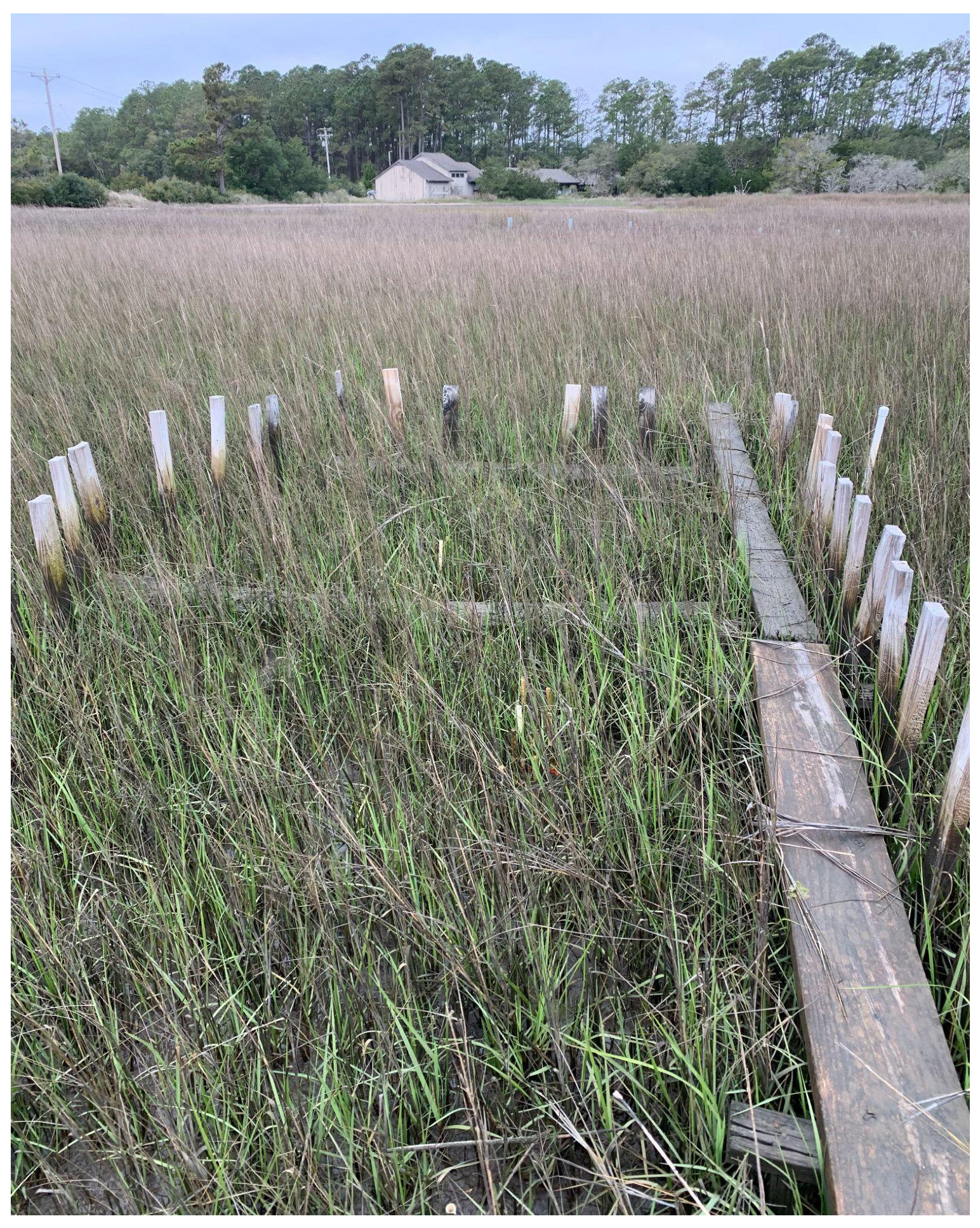
2.2.2. Non-Destructive Biomass Data Collection
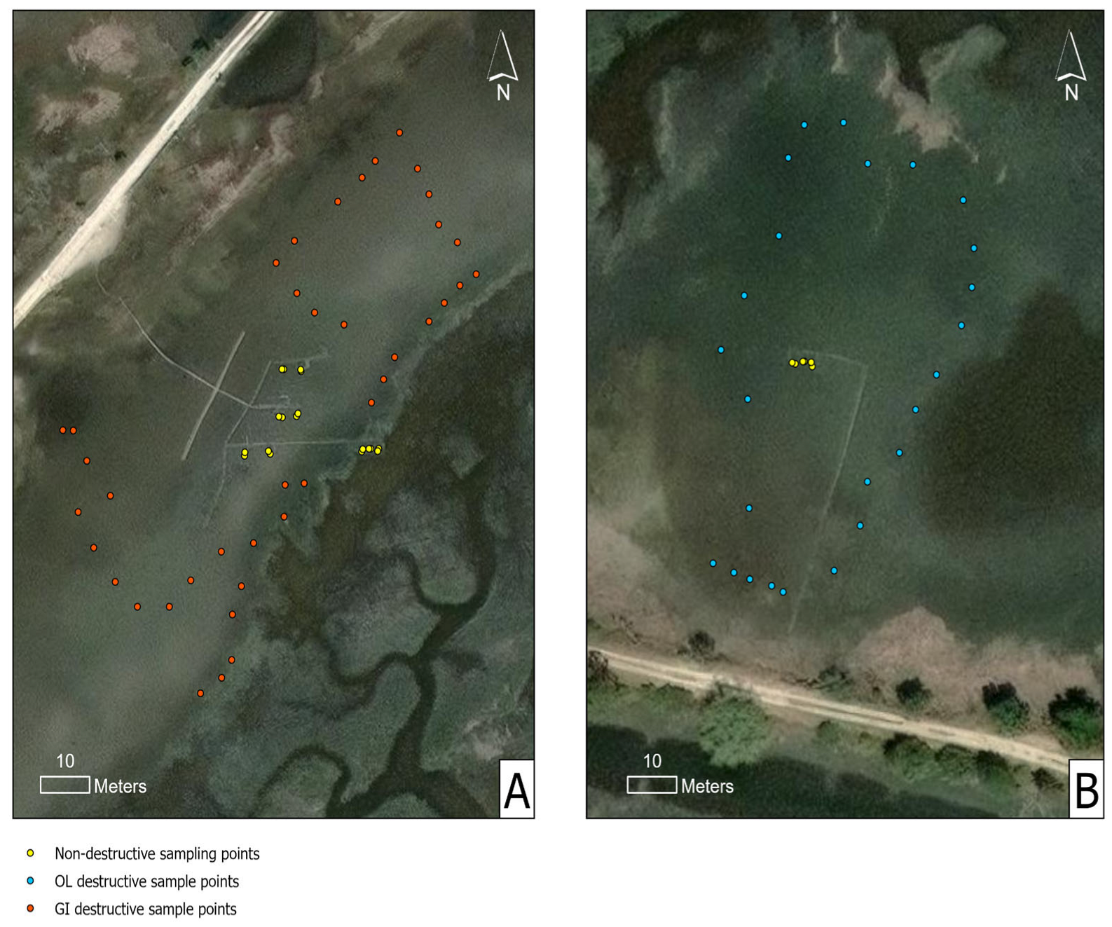
2.2.3. Destructive Biomass Data Collection
2.3. Approaches
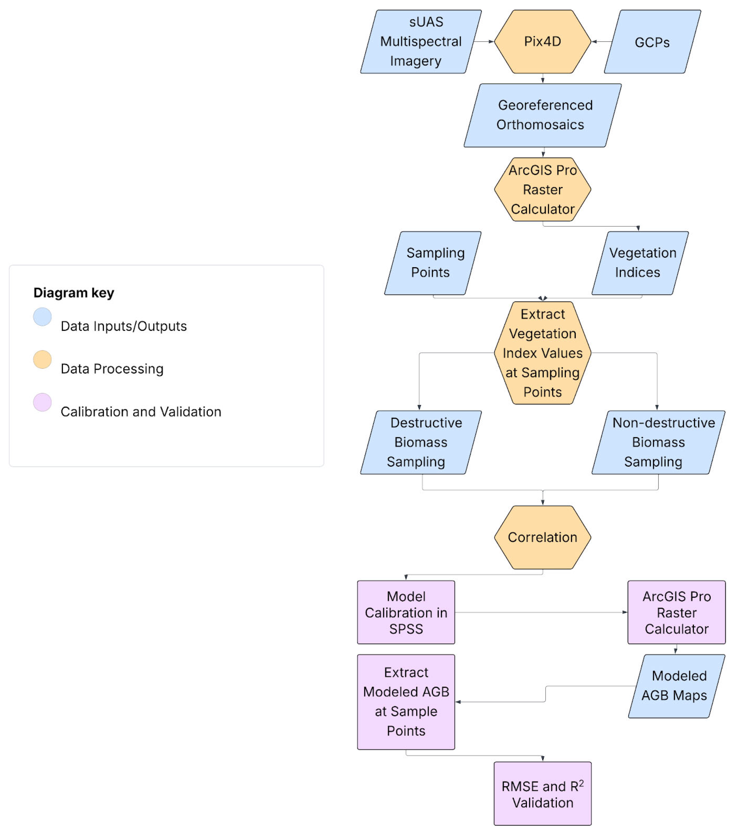
2.3.1. sUAS Data Processing
2.3.2. sUAS-Based Biomass Modeling
3. Results
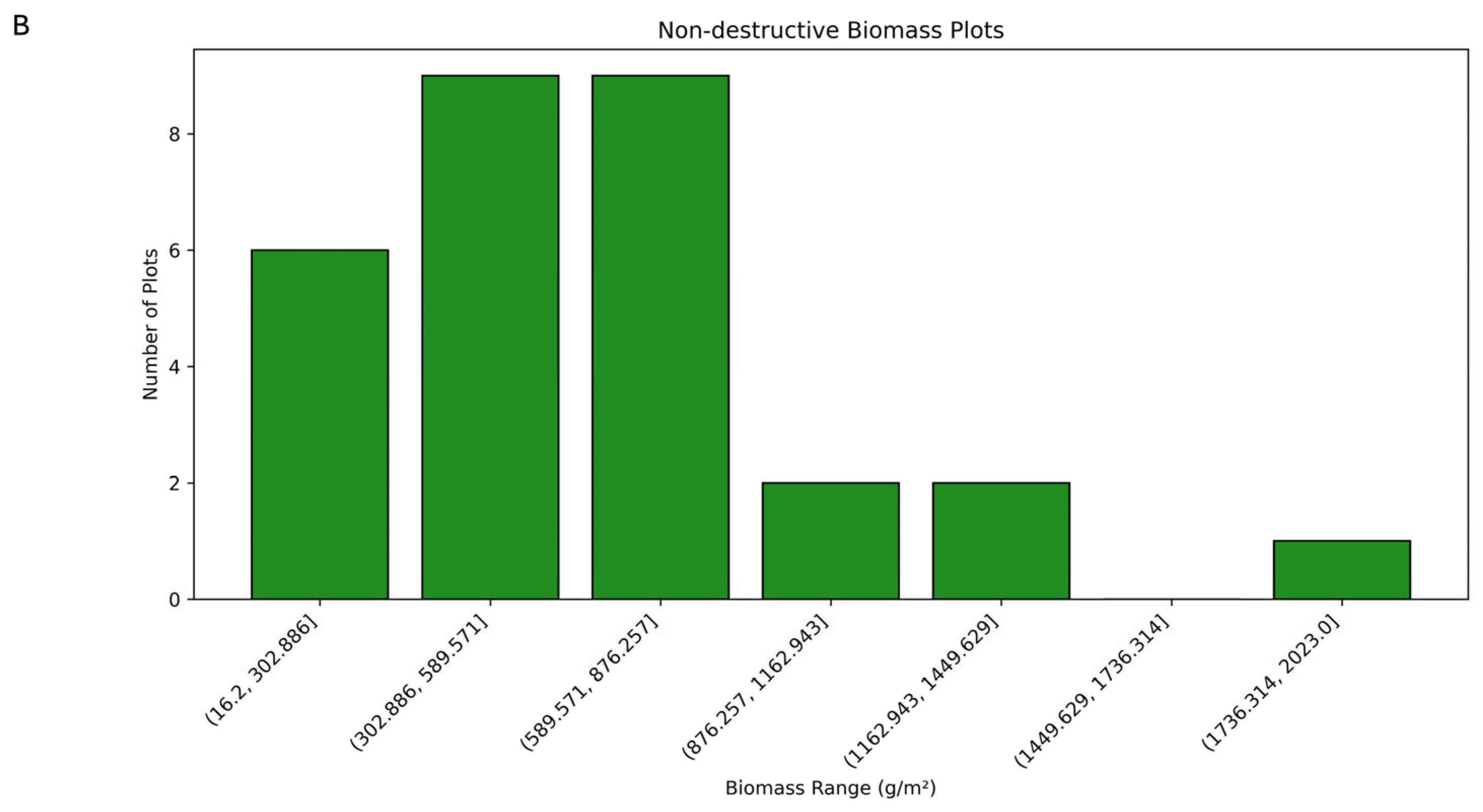
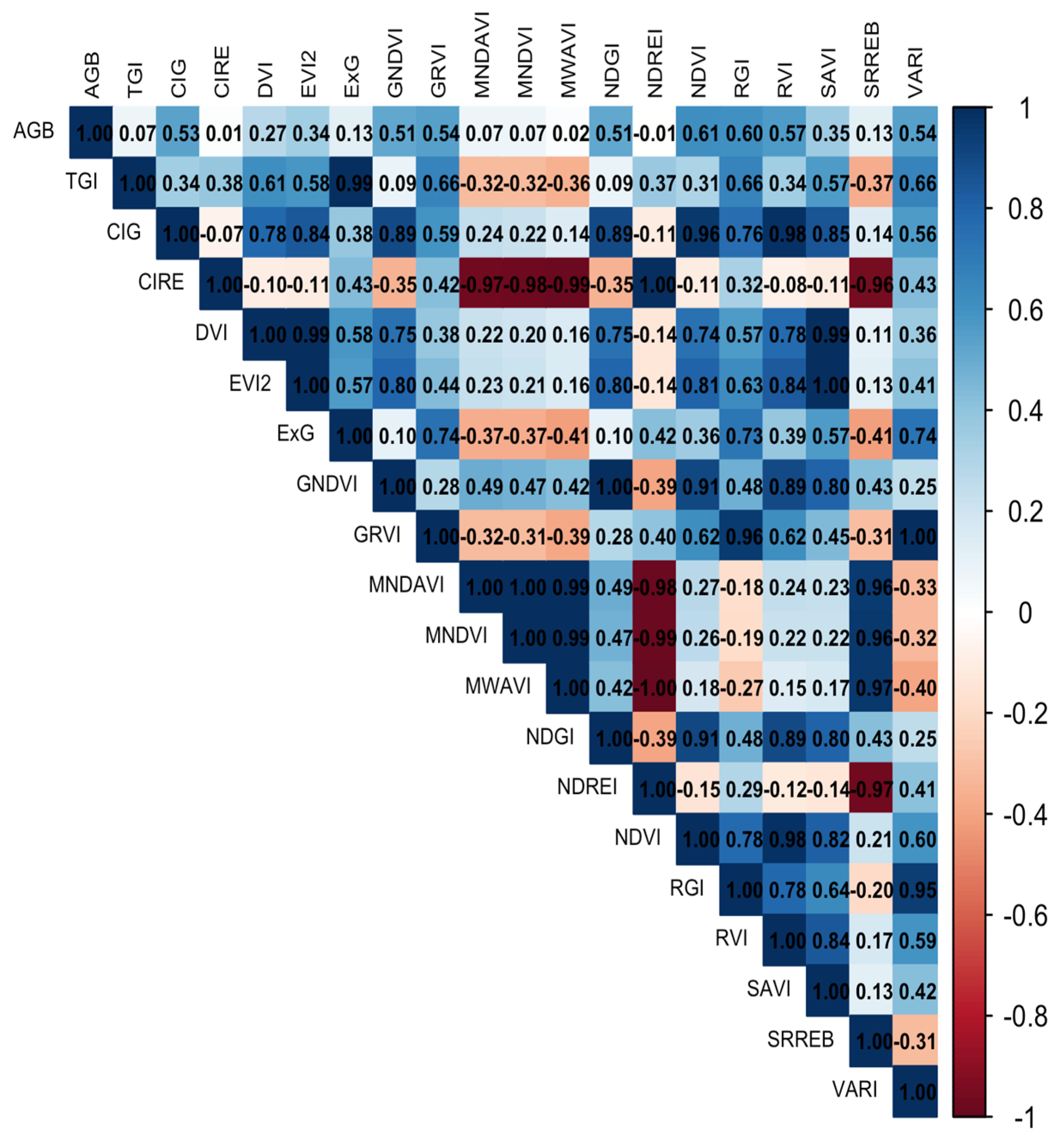
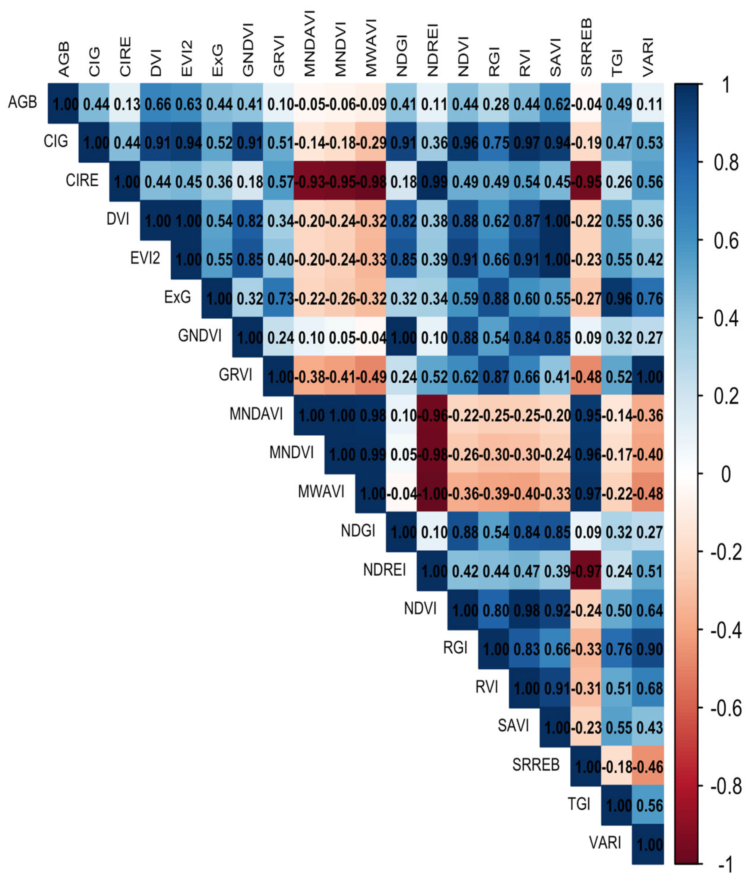
3.1. Biomass Values and Correlations for Destructive and Non-Destructive Samples
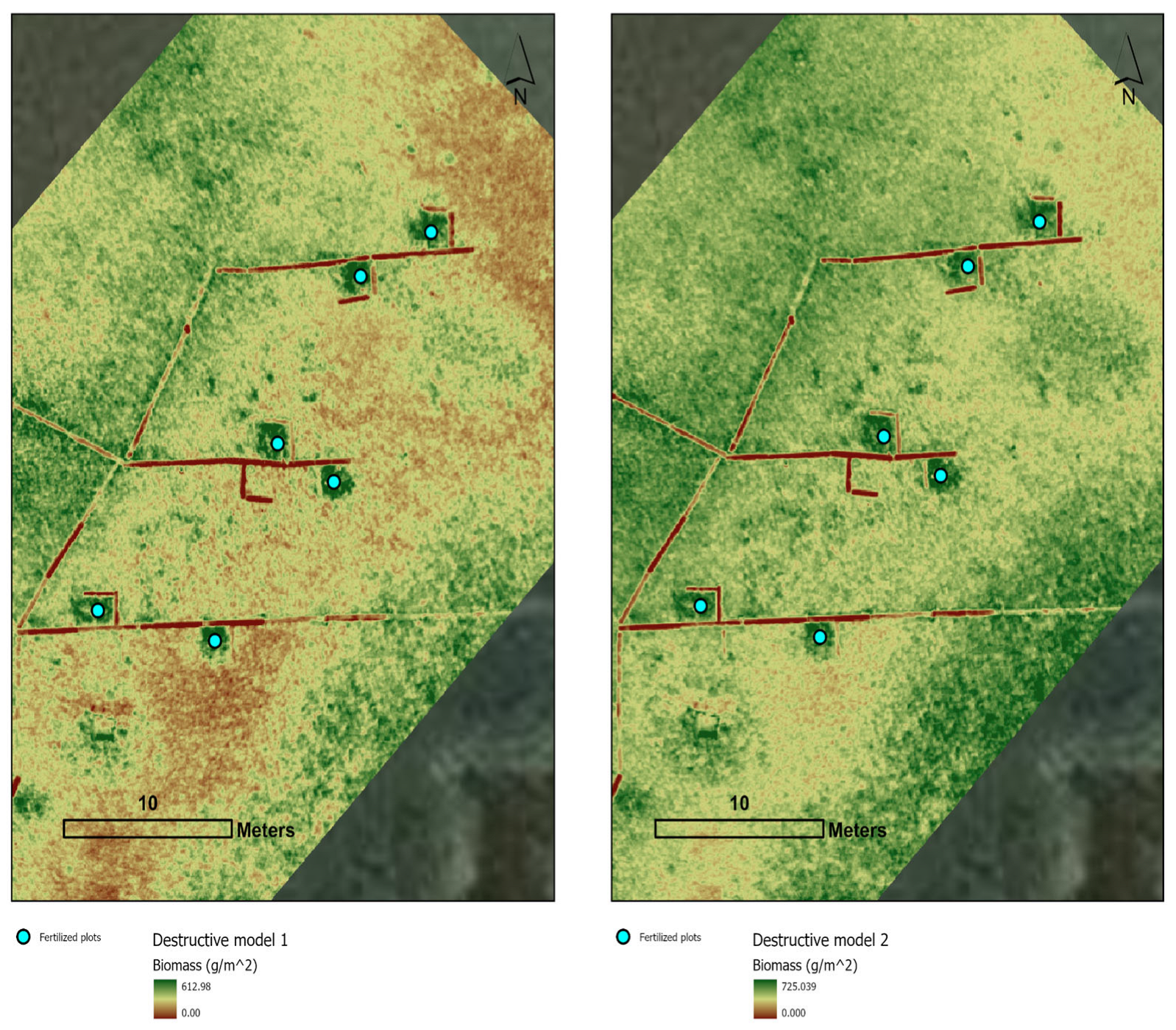
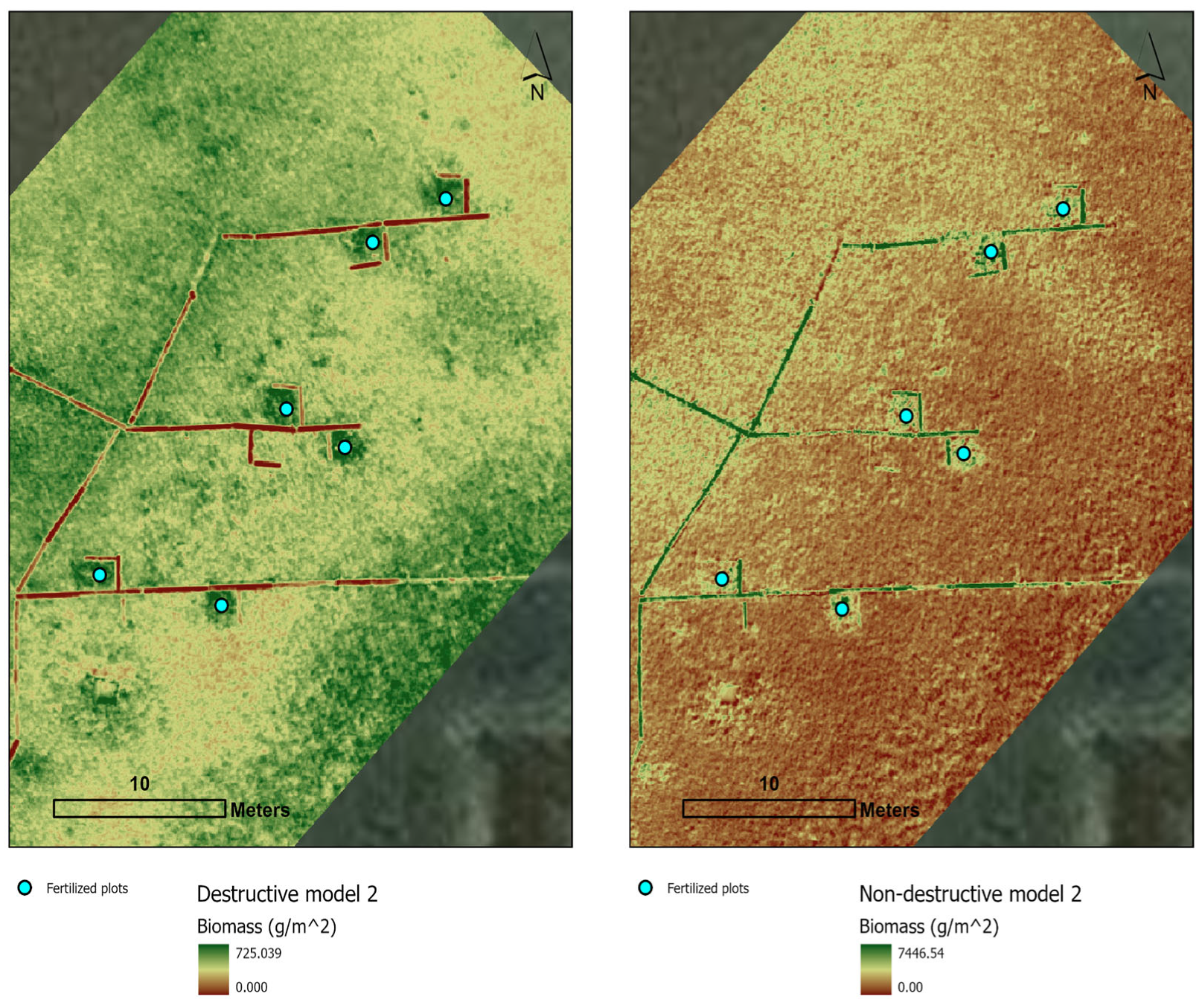
3.2. Models and Maps for Destructive and Non-Destructive Samples
3.3. Model Validation
4. Discussion
5. Conclusions
Author Contributions
Funding
Data Availability Statement
Acknowledgments
Conflicts of Interest
References
- Mitsch, W.J.; Gosselink, J.G. Wetlands, 5th ed.; John Wiley & Sons: Hoboken, NJ, USA, 2015. [Google Scholar]
- Turner, R.E.; Verhoeven, J.T.; Grobicki, A.; Davis, J.; Liu, S.R.; An, S.Q. The Changshu Declaration on wetlands: Final resolution adopted at the 10th INTECOL International Wetlands Conference, Changshu, People’s Republic of China, 19–24 September 2016. Ecol. Eng. 2017, 101, 1–2. [Google Scholar] [CrossRef]
- Sacande, M.; Martucci, A.; Vollrath, A. Monitoring Large-Scale Restoration Interventions from Land Preparation to Biomass Growth in the Sahel. Remote Sens. 2021, 13, 3767. [Google Scholar] [CrossRef]
- de Almeida, D.R.A.; Stark, S.C.; Valbuena, R.; Broadbent, E.N.; Silva, T.S.; de Resende, A.F.; Ferreira, M.P.; Cardil, A.; Silva, C.A.; Amazonas, N.; et al. A New Era in Forest Restoration Monitoring. Restor. Ecol. 2019, 28, 8–11. [Google Scholar] [CrossRef]
- Viani, R.A.; Barreto, T.E.; Farah, F.T.; Rodrigues, R.R.; Brancalion, P.H. Monitoring Young Tropical Forest Restoration Sites: How Much to Measure? Trop. Conserv. Sci. 2018, 11, 1940082918780916. [Google Scholar] [CrossRef]
- Conroy, B.M.; Hamylton, S.M.; Kumbier, K.; Kelleway, J.J. Assessing the structure of coastal forested wetland using field and remote sensing data. Estuar. Coast. Shelf Sci. 2022, 271, 107861. [Google Scholar] [CrossRef]
- Park, S.; Hwang, Y.; Lee, J.; Um, J. Evaluating operational potential of UAV transect mapping for wetland vegetation survey. J. Coast. Res. 2021, 114 (Suppl. S1), 474–478. [Google Scholar] [CrossRef]
- Abeysinghe, T.; Simic Milas, A.; Arend, K.; Hohman, B.; Reil, P.; Gregory, A.; Vázquez-Ortega, A. Mapping invasive Phragmites australis in the old woman creek estuary using UAV remote sensing and machine learning classifiers. Remote Sens. 2019, 11, 1380. [Google Scholar] [CrossRef]
- Amali, P.; Chow-Fraser, P.; Rupasinghe, P.A. Identification of most spectrally distinguishable phenological stage of invasive Phragmites australis in Lake Erie wetlands (Canada) for accurate mapping using multispectral satellite imagery. Wetl. Ecol. Manag. 2019, 27, 513–538. [Google Scholar] [CrossRef]
- Cao, J.; Leng, W.; Liu, K.; Liu, L.; He, Z.; Zhu, Y. Object-based mangrove species classification using unmanned aerial vehicle hyperspectral images and digital surface models. Remote Sens. 2018, 10, 89. [Google Scholar] [CrossRef]
- Mohler, R.L.; Morse, J.M. Using UAV imagery to map invasive Phragmites australis on the Crow Island State Game Area, Michigan, USA. Wetl. Ecol. Manag. 2022, 30, 1213–1229. [Google Scholar] [CrossRef]
- Pricope, N.G.; Halls, J.N.; Dalton, E.G.; Minei, A.; Chen, C.; Wang, Y. Precision mapping of coastal wetlands: An integrated remote sensing approach using unoccupied aerial systems light detection and ranging and multispectral data. J. Remote Sens. 2024, 4, 0169. [Google Scholar] [CrossRef]
- Rupasinghe, P.A.; Milas, A.S.; Arend, K.; Simonson, M.A.; Mayer, C.; Mackey, S. Classification of shoreline vegetation in the western basin of Lake Erie using airborne hyperspectral imager HSI2, Pleiades and UAV data. Int. J. Remote Sens. 2018, 40, 3008–3028. [Google Scholar] [CrossRef]
- Samiappan, S.; Turnage, G.; Hathcock, L.A.; Moorhead, R. Mapping of invasive Phragmites (common reed) in Gulf of Mexico coastal wetlands using multispectral imagery and small unmanned aerial systems. Int. J. Remote Sens. 2016, 38, 2861–2882. [Google Scholar] [CrossRef]
- Windle, A.E.; Staver, L.W.; Elmore, A.J.; Scherer, S.; Keller, S.; Malmgren, B.; Silsbe, G.M. Multi-temporal high-resolution marsh vegetation mapping using unoccupied aircraft system remote sensing and machine learning. Front. Remote Sens. 2023, 4, 1140999. [Google Scholar] [CrossRef]
- Zheng, J.; Hao, Y.; Wang, Y.; Zhou, S.; Wu, W.; Yuan, Q.; Gao, Y.; Guo, H.; Cai, X.; Zhao, B. Coastal wetland vegetation classification using pixel-based, object-based and deep learning methods based on RGB-UAV. Land 2022, 11, 2039. [Google Scholar] [CrossRef]
- Doughty, C.L.; Cavanaugh, K.C. Mapping coastal wetland biomass from high resolution unmanned aerial vehicle (UAV) imagery. Remote Sens. 2019, 11, 540. [Google Scholar] [CrossRef]
- Doughty, C.L.; Ambrose, R.F.; Okin, G.S.; Cavanaugh, K.C. Characterizing spatial variability in coastal wetland biomass across multiple scales using UAV and satellite imagery. Remote Sens. Ecol. Conserv. 2021, 7, 411–429. [Google Scholar] [CrossRef]
- Niu, X.; Chen, B.; Sun, W.; Feng, T.; Yang, X.; Liu, Y.; Liu, W.; Fu, B. Estimation of coastal wetland vegetation aboveground biomass by integrating UAV and satellite remote sensing data. Remote Sens. 2024, 16, 2760. [Google Scholar] [CrossRef]
- Martínez Prentice, R.; Villoslada, M.; Ward, R.D.; Bergamo, T.F.; Joyce, C.B.; Sepp, K. Synergistic use of Sentinel-2 and UAV-derived data for plant fractional cover distribution mapping of coastal meadows with digital elevation models. Biogeosciences 2024, 21, 1411–1431. [Google Scholar] [CrossRef]
- Wang, Z.; Ke, Y.; Lu, D.; Zhuo, Z.; Zhou, Q.; Han, Y.; Sun, P.; Gong, Z.; Zhou, D. Estimating fractional cover of saltmarsh vegetation species in coastal wetlands in the Yellow River Delta, China using ensemble learning model. Front. Mar. Sci. 2022, 9, 1077907. [Google Scholar] [CrossRef]
- Zhou, Z.; Yang, Y.; Chen, B. Estimating Spartina alterniflora fractional vegetation cover and aboveground biomass in a coastal wetland using SPOT6 satellite and UAV data. Aquat. Bot. 2017, 144, 38–45. [Google Scholar] [CrossRef]
- Curcio, A.C.; Peralta, G.; Aranda, M.; Barbero, L. Evaluating the performance of high spatial resolution UAV-photogrammetry and UAV-LiDAR for salt marshes: The Cádiz Bay study case. Remote Sens. 2022, 14, 3582. [Google Scholar] [CrossRef]
- White, L.; Ryerson, R.A.; Pasher, J.; Duffe, J. State of science assessment of remote sensing of great lakes coastal wetlands: Responding to an operational requirement. Remote Sens. 2020, 12, 3024. [Google Scholar] [CrossRef]
- Belloli, T.F.; de Arruda, D.C.; Guasselli, L.A.; Cunha, C.S.; Korb, C.C. Modeling wetland biomass and aboveground carbon: Influence of plot size and data treatment using remote sensing and random forest. Land 2025, 14, 616. [Google Scholar] [CrossRef]
- Lu, L.; Luo, J.; Xin, Y.; Duan, H.; Sun, Z.; Qiu, Y.; Xiao, Q. How can UAV contribute in satellite-based Phragmites australis aboveground biomass estimating? Int. J. Appl. Earth Obs. Geoinf. 2022, 114, 103024. [Google Scholar] [CrossRef]
- Xu, Y.; Qin, Y.; Li, B.; Li, J. Estimating vegetation aboveground biomass in Yellow River Delta coastal wetlands using Sentinel-1, Sentinel-2 and Landsat-8 imagery. Ecol. Inform. 2025, 87, 103096. [Google Scholar] [CrossRef]
- Alvarez-Vanhard, E.; Houet, T.; Mony, C.; Lecoq, L.; Corpetti, T. Can UAVs fill the gap between in situ surveys and satellites for habitat mapping? Remote Sens. Environ. 2020, 243, 111780. [Google Scholar] [CrossRef]
- Morgan, G.R.; Wang, C.; Morris, J.T. RGB Indices and Canopy Height Modelling for Mapping Tidal Marsh Biomass from a Small Unmanned Aerial System. Remote Sens. 2021, 13, 3406. [Google Scholar] [CrossRef]
- Lishawa, S.C.; Carson, B.D.; Brandt, J.S.; Tallant, J.M.; Reo, N.J.; Albert, D.A.; Monks, A.M.; Lautenbach, J.M.; Clark, E. Mechanical harvesting effectively controls young Typha spp. invasion and unmanned aerial vehicle data enhances post-treatment monitoring. Front. Plant Sci. 2017, 8, 619. [Google Scholar] [CrossRef]
- Shew, D.M.; Linthurst, R.A.; Seneca, E.D. Comparison of production computation methods in a southeastern North Carolina Spartina alterniflora salt marsh. Estuaries 1981, 4, 97–109. [Google Scholar] [CrossRef]
- Ge, C.; Zhang, C.; Zhang, Y.; Fan, Z.; Kong, M.; He, W. Synergy of UAV-LiDAR Data and Multispectral Remote Sensing Images for allometric estimation of Phragmites australis aboveground biomass in coastal wetland. Remote Sens. 2024, 16, 3073. [Google Scholar] [CrossRef]
- Fehrmann, L.; Kleinn, C. General Considerations about the Use of Allometric Equations for Biomass Estimation on the Example of Norway Spruce in Central Europe. For. Ecol. Manag. 2006, 236, 412–421. [Google Scholar] [CrossRef]
- Djomo, A.N.; Ibrahima, A.; Saborowski, J.; Gravenhorst, G. Allometric Equations for Biomass Estimations in Cameroon and Pan Moist Tropical Equations Including Biomass Data from Africa. For. Ecol. Manag. 2010, 260, 1873–1885. [Google Scholar] [CrossRef]
- Kuyah, S.; Dietz, J.; Muthuri, C.; Jamnadass, R.; Mwangi, P.; Coe, R.; Neufeldt, H. Allometric Equations for Estimating Biomass in Agricultural Landscapes: II. Belowground Biomass. Agric. Ecosyst. Environ. 2012, 158, 225–234. [Google Scholar] [CrossRef]
- Kebede, B.; Soromessa, T. Allometric Equations for Aboveground Biomass Estimation of Olea europaea l. Subsp. Cuspidata in Mana Angetu Forest. Ecosyst. Health Sustain. 2018, 4, 1433951. [Google Scholar] [CrossRef]
- Morris, J.T.; Haskin, B. A 5-yr record of aerial primary production and stand characteristics of Spartina alterniflora. Ecology 1990, 71, 2209–2217. [Google Scholar] [CrossRef]
- Dickerman, J.A.; Stewart, A.J.; Wetzel, R.G. Estimates of net annual aboveground production: Sensitivity to sampling frequency. Ecology 1986, 67, 650–659. [Google Scholar] [CrossRef]
- National Science Foundation. CAREER: Wetland Remote Sensing Using Drones for Carbon and Biomass Monitoring (Award No. 2348767). 2023. Available online: https://www.nsf.gov/awardsearch/showAward?AWD_ID=2348767 (accessed on 12 January 2025).
- Morris, J.; Sundberg, K. LTREB: Aboveground Biomass, Plant Density, Annual Aboveground Productivity, and Plant Heights in Control and Fertilized Plots in a Spartina Alterniflora-Dominated Salt Marsh, North Inlet, Georgetown, SC: 1984–2020; Ver 5; Environmental Data Initiative: Albuquerque, NM, USA, 2021. [Google Scholar] [CrossRef]
- Zhou, R.; Yang, C.; Li, E.; Cai, X.; Wang, X. Aboveground biomass estimation of wetland vegetation at the species level using unoccupied aerial vehicle RGB imagery. Front. Plant Sci. 2023, 14, 1181887. [Google Scholar] [CrossRef] [PubMed]
- Wu, N.; Zhang, C.; Zhuo, W.; Shi, R.; Zhu, F.; Liu, S. Assessment of the impact of coastal wetland saltmarsh vegetation types on aboveground biomass inversion. Remote Sens. 2024, 16, 4762. [Google Scholar] [CrossRef]
- Morgan, G.R.; Hodgson, M.E.; Wang, C.; Schill, S.R. Unmanned Aerial Remote Sensing of Coastal Vegetation: A Review. Ann. GIS 2022, 28, 385–399. [Google Scholar] [CrossRef]
- Taddia, Y.; Pellegrinelli, A.; Corbau, C.; Franchi, G.; Staver, L.W.; Stevenson, J.C.; Nardin, W. High-Resolution Monitoring of Tidal Systems Using UAV: A Case Study on Poplar Island, Md (USA). Remote Sens. 2021, 13, 1364. [Google Scholar] [CrossRef]
- Dai, W.; Li, H.; Chen, X.; Xu, F.; Zhou, Z.; Zhang, C. Saltmarsh Expansion in Response to Morphodynamic Evolution: Field Observations in the Jiangsu Coast Using UAV. J. Coast. Res. 2020, 95 (Suppl. S1), 433–437. [Google Scholar] [CrossRef]
- Barr, J.R.; Green, M.C.; DeMaso, S.J.; Hardy, T.B. Detectability and Visibility Biases Associated with Using a Consumer-grade Unmanned Aircraft to Survey NESTING Colonial Waterbirds. J. Field Ornithol. 2018, 89, 242–257. [Google Scholar] [CrossRef]
- Boon, M.A.; Drijfhout, A.P.; Tesfamichael, S. Comparison of A Fixed Wing and Multi-rotor Uav for Environmental Mapping Applications: A Case Study. Int. Arch. Photogramm. Remote Sens. Spat. Inf. Sci. 2017, XLII-2, 47–54. [Google Scholar] [CrossRef]
- Farris, A.S.; Defne, Z.; Ganju, N.K. Identifying Salt Marsh Shorelines from Remotely Sensed Elevation Data and Imagery. Remote Sens. 2019, 11, 1795. [Google Scholar] [CrossRef]
- Pinton, D.; Canestrelli, A.; Wilkinson, B.; Ifju, P.; Ortega, A. A New Algorithm for Estimating Ground Elevation and Vegetation Characteristics in Coastal Salt Marshes from High-resolution Uav-based Lidar Point Clouds. Earth Surf. Process. Landf. 2020, 45, 3687–3701. [Google Scholar] [CrossRef]
- Yi, W.; Wang, N.; Yu, H.; Jiang, Y.; Zhang, D.; Li, X.; Lv, L.; Xie, Z. An enhanced monitoring method for spatio-temporal dynamics of salt marsh vegetation using Google Scholar Earth Engine. Estuar. Coast. Shelf Sci. 2024, 298, 108658. [Google Scholar] [CrossRef]
- Sun, S.; Wang, Y.; Song, Z.; Chen, C.; Zhang, Y.; Chen, X.; Chen, W.; Yuan, W.; Wu, X.; Ran, X.; et al. Modelling aboveground biomass carbon stock of the Bohai Rim Coastal Wetlands by integrating remote sensing, terrain, and climate data. Remote Sens. 2021, 13, 4321. [Google Scholar] [CrossRef]
- Curcio, A.C.; Barbero, L.; Peralta, G. Enhancing salt marshes monitoring: Estimating biomass with drone-derived habitat-specific models. Remote Sens. Appl. Soc. Environ. 2024, 35, 101216. [Google Scholar] [CrossRef]
- Lumbierres, M.; Méndez, P.F.; Bustamante, J.; Soriguer, R.; Santamaría, L. Modeling biomass production in seasonal wetlands using MODIS NDVI land surface phenology. Remote Sens. 2017, 9, 392. [Google Scholar] [CrossRef]


| Index | Equation | Sources |
|---|---|---|
| Normalized Difference Vegetation Index | [30,44,45] | |
| Visible Atmospherically Resistant Index 2 | [46,47] | |
| Soil-Adjusted Vegetation Index 1 | [13,45] | |
| Simple Ratio | Ratio between any two bands. Example: | [48,49] |
| Chlorophyll Index Green | [30] | |
| Chlorophyll Index RedEdge | [30] | |
| Difference Vegetation Index | [45] | |
| Enhanced Vegetation Index 2 | [30] | |
| Excess Green Index 2 | [47] | |
| Relative Green Index 2 | [47] | |
| Green Normalized Difference Vegetation Index | [30] | |
| Green-Red Vegetation Index 2 | [47] | |
| Modified Normalized Difference Aquatic Vegetation Index | [49] | |
| Modified Normalized Difference Vegetation Index | [49] | |
| Modified Water-Adjusted Vegetation Index 1 | [49] | |
| Normalized Difference Green Index | [48] | |
| Normalized Difference Red Edge Index | [48] | |
| Ratio Vegetation Index | [45] | |
| Triangular Greenness Index 2 | [46] |
| Models | Variables | Equation | R2 |
|---|---|---|---|
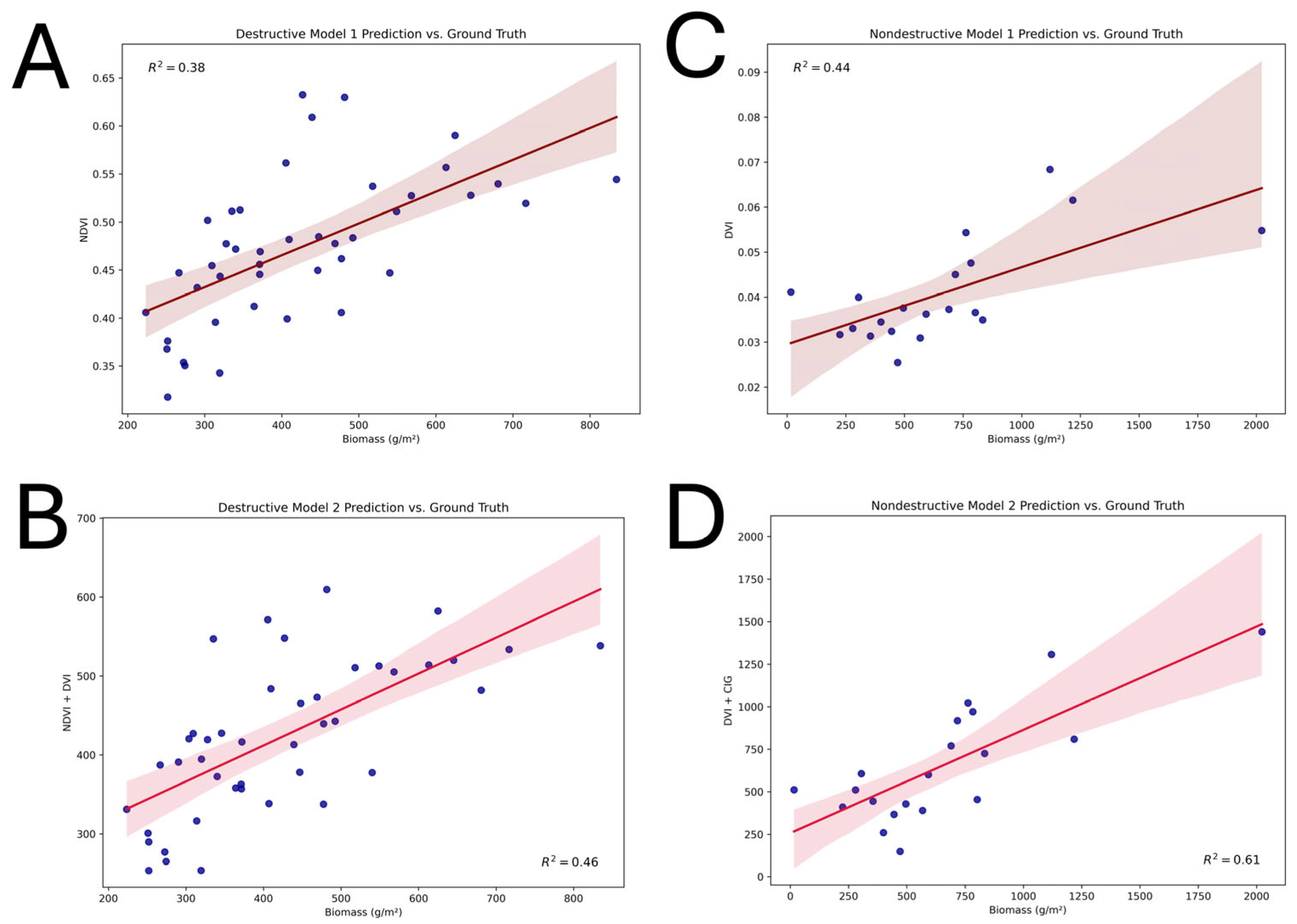
| Destructive Samples Model 1 | NDVI | AGB = −115.094 + 1136.393(NDVI) | 0.38 |
| Destructive Samples Model 2 | NDVI, DVI | AGB = −147.314 + 1716.872(NDVI) − 3759.493(DVI) | 0.46 |
| Non-Destructive Samples Model 1 | DVI | AGB = −395.775 + 25792.653(DVI) | 0.44 |
| Non-Destructive Samples Model 2 | DVI, CIG | AGB = −862.319 + 61084.777(DVI) − 748.207(CIG) | 0.61 |
| Models | Variables | Validation RMSE (g/m2) |
|---|---|---|
| Destructive Samples Model 1 | NDVI | 73.17 |
| Destructive Samples Model 2 | NDVI, DVI | 70.91 |
| Non-Destructive Samples Model 1 | DVI | 344.73 |
| Non-Destructive Samples Model 2 | DVI, CIG | 214.86 |
Disclaimer/Publisher’s Note: The statements, opinions and data contained in all publications are solely those of the individual author(s) and contributor(s) and not of MDPI and/or the editor(s). MDPI and/or the editor(s) disclaim responsibility for any injury to people or property resulting from any ideas, methods, instructions or products referred to in the content. |
© 2025 by the authors. Licensee MDPI, Basel, Switzerland. This article is an open access article distributed under the terms and conditions of the Creative Commons Attribution (CC BY) license (https://creativecommons.org/licenses/by/4.0/).
Share and Cite
Morgan, G.R.; Stevenson, L.; Wang, C.; Avtar, R. UAS Remote Sensing for Coastal Wetland Vegetation Biomass Estimation: A Destructive vs. Non-Destructive Sampling Experiment. Remote Sens. 2025, 17, 2335. https://doi.org/10.3390/rs17142335
Morgan GR, Stevenson L, Wang C, Avtar R. UAS Remote Sensing for Coastal Wetland Vegetation Biomass Estimation: A Destructive vs. Non-Destructive Sampling Experiment. Remote Sensing. 2025; 17(14):2335. https://doi.org/10.3390/rs17142335
Chicago/Turabian StyleMorgan, Grayson R., Lane Stevenson, Cuizhen Wang, and Ram Avtar. 2025. "UAS Remote Sensing for Coastal Wetland Vegetation Biomass Estimation: A Destructive vs. Non-Destructive Sampling Experiment" Remote Sensing 17, no. 14: 2335. https://doi.org/10.3390/rs17142335
APA StyleMorgan, G. R., Stevenson, L., Wang, C., & Avtar, R. (2025). UAS Remote Sensing for Coastal Wetland Vegetation Biomass Estimation: A Destructive vs. Non-Destructive Sampling Experiment. Remote Sensing, 17(14), 2335. https://doi.org/10.3390/rs17142335