

Principles of Correction for Long-Term Orbital Observations of Atmospheric Composition, Applied to AIRS v.6 CH4 and CO Data
 ,
,  ,
,
Abstract
1. Introduction
2. Materials and Methods
- P—atmospheric pressure at the station level, mbar
- P0—atmospheric pressure at sea level equal to 1013 mbar
- P is pressure in the layer of given height h;
- P0—pressure at sea level;
- h − h0—height difference equal to h when calculated for sea level, m;
- R—universal gas constant;
- T—absolute temperature in Kelvin degrees;
- M—molar mass of air;
- g—gravitational acceleration.
- a is the slope coefficient (hereinafter SC) of the regression
- b is the shift coefficient (error term) of the regression.
3. Results
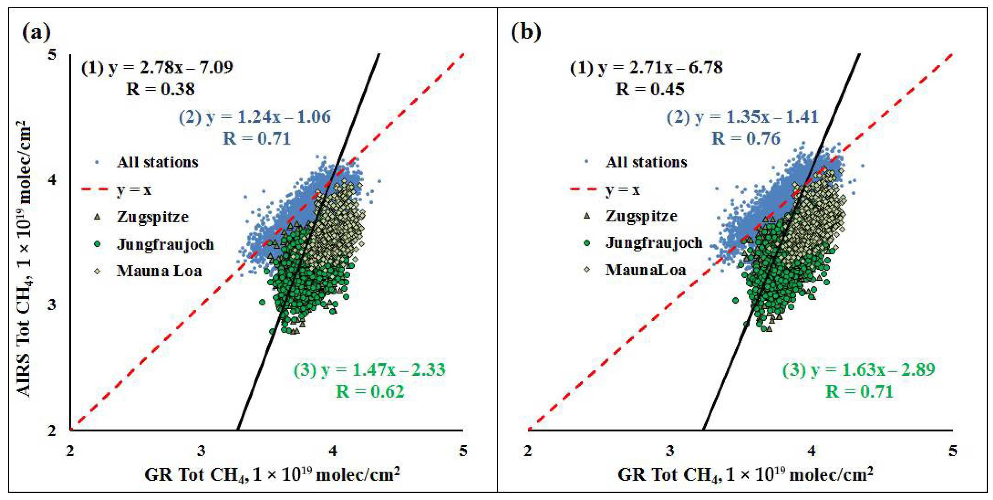
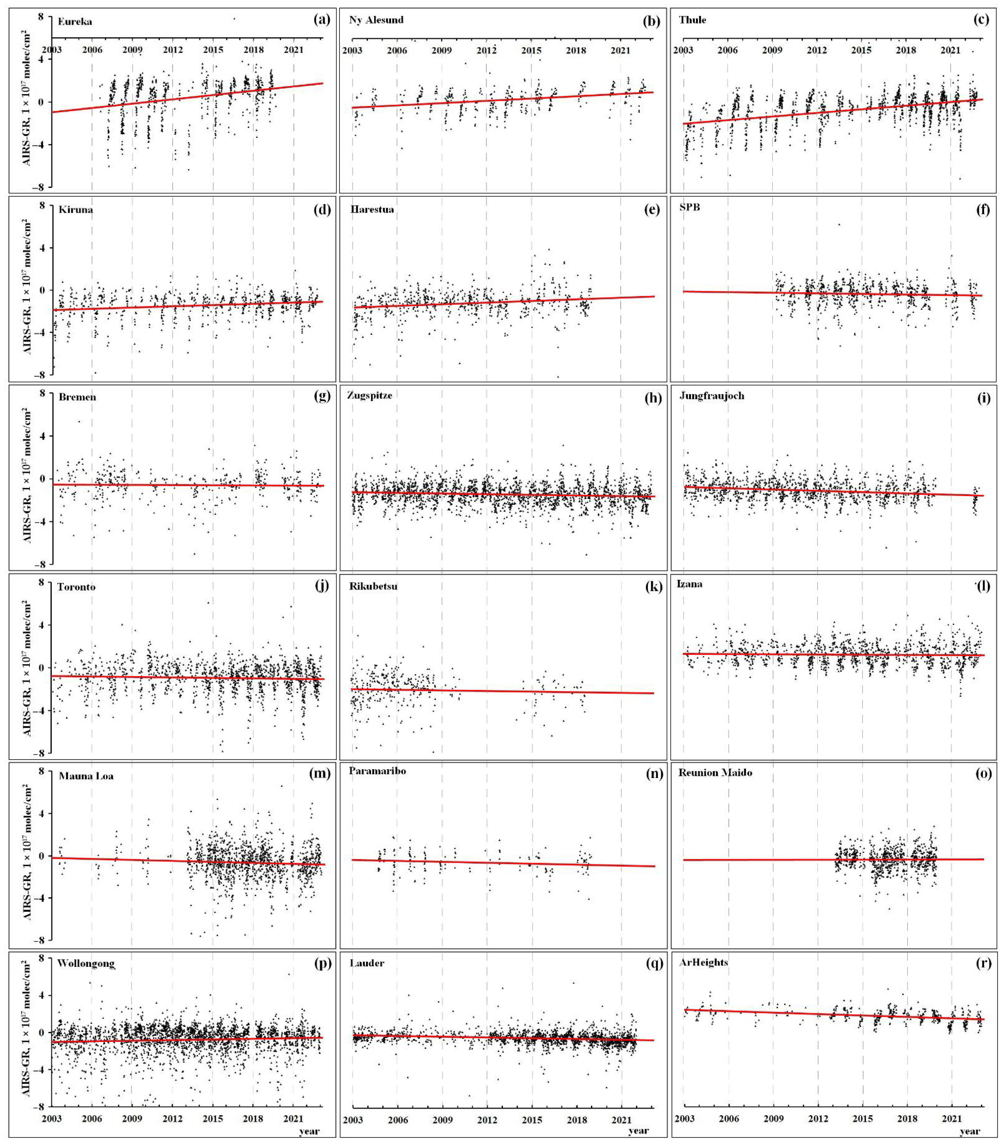
3.1. AIRS v.6 CH4 TC Product
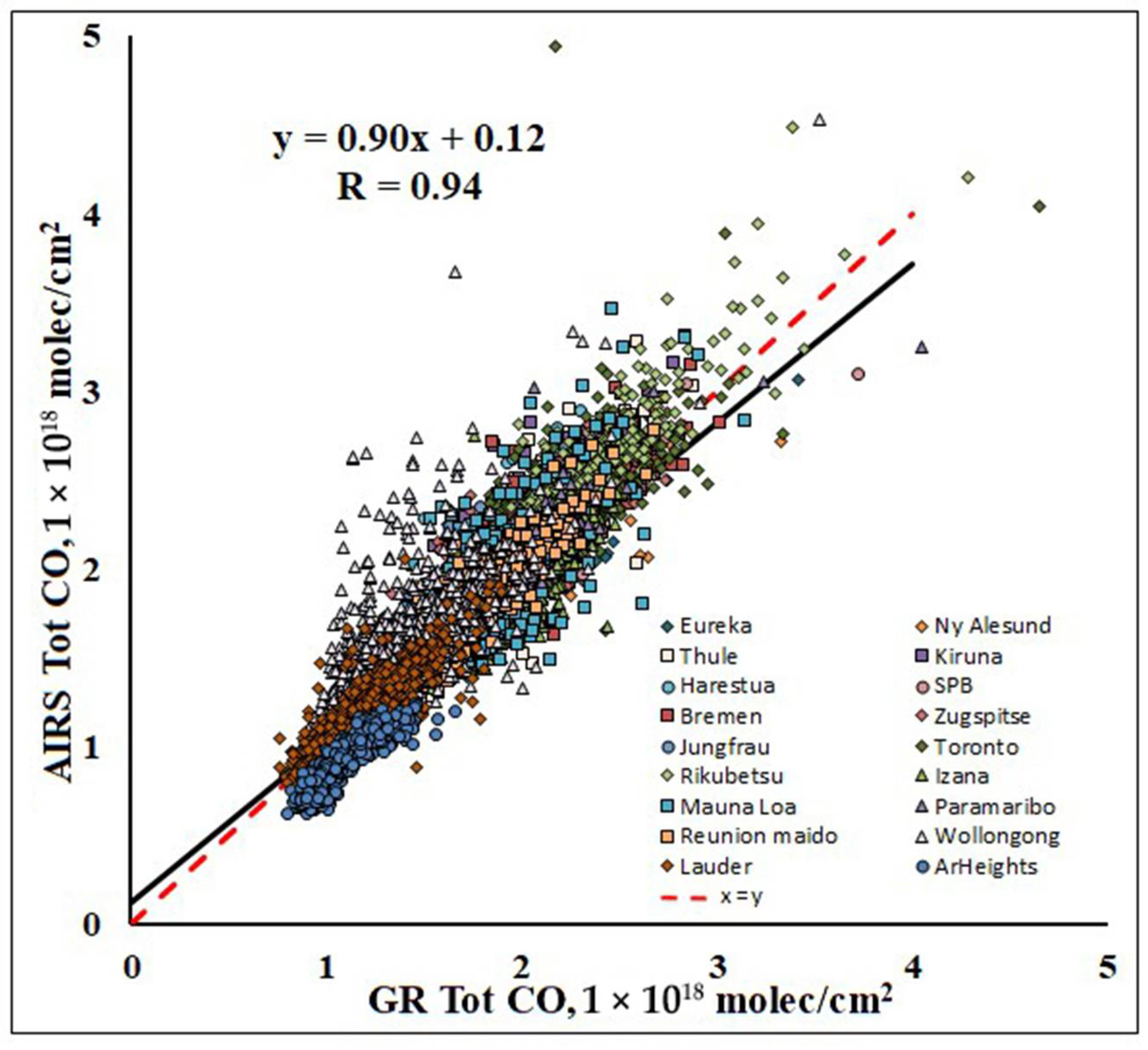
3.2. AIRS v.6 CO TC Product
4. Discussion
5. Conclusions
Supplementary Materials
Author Contributions
Funding
Data Availability Statement
Acknowledgments
Conflicts of Interest
Abbreviations
| AIRS | Atmospheric InfraRed Sounder |
| TC | Total Column |
| NDACC | Network for the Detection of Atmospheric Composition Change |
| OCO | Orbiting Carbon Observatory |
| MOPITT | Measurements Of Pollution In The Troposphere |
| MODIS | MOderate Resolution Imaging Spectroradiometer |
| OMI | Ozone Monitoring Instrument |
| IASI | Infrared Atmospheric Sounding Interferometer |
| NASA | National Aeronautics and Space Administration |
| TCCON | Total Carbon Column Observing Network |
| TROPOMI | TROPOspheric Monitoring Instrument |
| VMR | Volume Mixing Ratio |
| FTIR | Fourier Transform InfraRed spectrometer |
| SC | Slope Coefficient |
| SSD | Satellite Spectrometer Drift |
References
- Eldering, A.; O’Dell, C.W.O.; Wennberg, P.; Crisp, D.; Gunson, M.R.; Viatte, C.; Avis, C.; Braverman, A.; Castano, R.; Chang, A.; et al. The Orbiting Carbon Observatory-2: First 18 months of science data products. Atmos. Meas. Tech. 2017, 10, 549–563. [Google Scholar] [CrossRef]
- Orbiting Carbon Observatory 3, National Aeronautics and Space Administration. 2019. Available online: https://d2pn8kiwq2w21t.cloudfront.net/documents/oco-3-fact-sheet-4-pages.pdf (accessed on 2 February 2025).
- Jiang, Z.; Worden, J.R.; Worden, H.; Deeter, M.; Jones, D.B.A.; Arellano, A.F.; Henze, D.K. A fifteen-year record of CO emissions constrained by MOPITT CO observations. Atmos. Chem. Phys. 2017, 17, 4565–4583. [Google Scholar] [CrossRef]
- Fortems-Cheiney, A.; Broquet, G.; Pison, I.; Saunois, M.; Potier, E.; Berchet, A.; Dufour, G.; Siour, G.; Denier van der Gon, H.; Dellaert, S.N.C.; et al. Analysis of the anthropogenic and biogenic NOx emissions over 2008–2017: Assessment of the trends in the 30 most populated urban areas in Europe. Geophys. Res. Lett. 2021, 48, e2020GL092206. [Google Scholar] [CrossRef]
- Buchholz, R.R.; Worden, H.M.; Park, M.; Francis, G.; Deeter, M.N.; Edwards, D.P.; Emmons, L.K.; Gaubert, B.; Gille, J.; Martínez-Alonso, S.; et al. Air pollution trends measured from Terra: CO and AOD over industrial, fire-prone, and background regions. Remote Sens. Environ. 2021, 256, 112275. [Google Scholar] [CrossRef]
- Yurganov, L.; Rakitin, V. Two decades of satellite observations of carbon monoxide confirm the increase in Northern Hemispheric Wildfires. Atmosphere 2022, 13, 1479. [Google Scholar] [CrossRef]
- Jiang, Z.; Zhu, R.; Miyazaki, K.; McDonald, B.C.; Klimont, Z.; Zheng, B.; Boersma, K.F.; Zhang, Q.; Worden, H.; Worden, J.R.; et al. Decadal variabilities in tropospheric nitrogen oxides over United States, Europe, and China. J. Geophys. Res. Atmos. 2022, 127, e2021JD035872. [Google Scholar] [CrossRef]
- Jin, X.; Zhu, Q.; Cohen, R.C. Direct estimates of biomass burning NOx emissions and lifetimes using daily observations from TROPOMI. Atmos. Chem. Phys. 2021, 21, 15569–15587. [Google Scholar] [CrossRef]
- Schmidt, A.; Leadbetter, S.; Theys, N.; Carboni, E.; Witham, C.S.; Stevenson, J.A.; Birch, C.E.; Thordarson, T.; Turnock, S.; Barsotti, S.; et al. Satellite detection, long-range transport, and air quality impacts of volcanic sulfur dioxide from the 2014–2015 flood lava eruption at Bárðarbunga (Iceland). J. Geophys. Res. Atmos. 2015, 120, 9739–9757. [Google Scholar] [CrossRef]
- Huang, M.; Carmichael, G.R.; Pierce, R.B.; Jo, D.S.; Park, R.J.; Flemming, J.; Emmons, L.K.; Bowman, K.W.; Henze, D.K.; Davila, Y.; et al. Impact of intercontinental pollution transport on North American ozone air pollution: An HTAP phase 2 multi-model study. Atmos. Chem. Phys. 2017, 17, 5721–5750. [Google Scholar] [CrossRef]
- Hu, Q.; Goloub Ph Veselovskii, I.; Bravo-Aranda, J.-A.; Popovici, I.E.; Podvin, T.; Haeffelin, M.; Lopatin, A.; Dubovik, O.; Pietras, C.; Huang, X.; et al. Long-range-transported Canadian smoke plumes in the lower stratosphere over northern France. Atmos. Chem. Phys. 2019, 19, 1173–1193. [Google Scholar] [CrossRef]
- Yurganov, L.N.; McMillan, W.W.; Dzhola, A.V.; Grechko, E.I.; Global, A.I.R.S.; Yurganov, L.N.; McMillan, W.W.; Dzhola, A.V.; Grechko, E.I. Global AIRS and MOPITT CO measurements: Validation, comparison, and links to biomass burning variations and carbon cycle. J. Geophys. Res. 2008, 113, D09301. [Google Scholar] [CrossRef]
- Hegarty, J.D.; Cady-Pereira, K.E.; Payne, V.H.; Kulawik, S.S.; Worden, J.R.; Kantchev, V.; Worden, H.M.; McKain, K.; Pittman, J.V.; Commane, R.; et al. Validation and error estimation of AIRS MUSES CO profiles with HIPPO, ATom, and NOAA GML aircraft observations. Atmos. Meas. Tech. 2022, 15, 205–223. [Google Scholar] [CrossRef]
- Gruzdev, A.N.; Elohov, A.S. Comparison of data of OMI long-term measurements of NO2 contents in the stratosphere and troposphere with the results of ground-based measurements. Izv. Atmos. Ocean. Phys. 2023, 59, 78–99. [Google Scholar] [CrossRef]
- Aumann, H.H.; Chahine, M.T.; Gautier, C.; Goldberg, M.; Kalnay, E.; McMillin, L.; Revercomb, H.; Rosenkranz, P.W.; Smith, W.L.; Staelin, D.; et al. AIRS/AMSU/HSB on the Aqua mission: Design, science objectives, data products and processing systems. IEEE Trans. Geosci. Remote Sens. 2003, 41, 253–264. [Google Scholar] [CrossRef]
- Susskind, J.; Blaisdell, J.M.; Iredell, L.; Susskind, J.; Blaisdell, J.M.; Iredell, L. Improved methodology for surface atmospheric soundings error estimates quality control procedures: The atmospheric infrared sounder science team version-6 retrieval algorithm. J. Appl. Remote Sens. 2014, 8, 084994. [Google Scholar] [CrossRef]
- Rakitin, V.S.; Shtabkin Yu, A.; Elansky, N.F.; Pankratova, N.V.; Skorokhod, A.I.; Grechko, E.I.; Safronov, A.N. Comparison results of satellite and ground-based spectroscopic measurements of CO, CH4, and CO2 total contents. Atmos. Ocean. Opt. 2015, 28, 533–542. [Google Scholar] [CrossRef]
- Wang, P.; Elansky, N.F.; Timofeev Yu, M.; Wang, G.; Golitsyn, G.S.; Makarova, M.V.; Rakitin, V.S.; Stabkin Yu Skorokhod, A.I.; Grechko, E.I.; Fokeeva, E.V.; et al. Long-term trends of carbon monoxide total columnar amount in urban areas and background regions: Ground-and satellite-based spectroscopic measurements. Adv. Atmos. Sci. 2018, 35, 785–795. [Google Scholar] [CrossRef]
- Krol, M.; Peters, W.; Hooghiemstra, P.; George, M.; Clerbaux, C.; Hurtmans, D.; McInerney, D.; Sedano, F.; Bergamaschi, P.; El Hajj, M.; et al. How much CO was emitted by the 2010 fires around Moscow? Atmos. Chem. Phys. 2013, 13, 4737–4747. [Google Scholar] [CrossRef]
- Yurganov, L.N.; Rakitin, V.; Dzhola, A.; August, T.; Fokeeva, E.; George, M.; Gorchakov, G.; Grechko, E.; Hannon, S.; Karpov, A.; et al. Satellite-and ground-based CO total column observations over 2010 Russian fires: Accuracy of top-down estimates based on thermal IR satellite data. Atmos. Chem. Phys. 2011, 11, 7925–7942. [Google Scholar] [CrossRef]
- Safronov, A.N.; Fokeeva, E.V.; Rakitin, V.S.; Grechko, E.I.; Shumskii, R.A. Severe wildfires near Moscow, Russia, in 2010: Modeling of carbon monoxide pollution and comparisons with observations. Remote Sens. 2015, 7, 395–429. [Google Scholar] [CrossRef]
- Abed, F.G.; Al-Salihi, A.M.; Rajab, J.M. Space-borne observation of methane from atmospheric infrared sounder: Data analysis and distribution over Iraq. J. Appl. Adv. Res. 2017, 4, 256–264. [Google Scholar] [CrossRef]
- Zou, M.; Xiong, X.; Wu, Z.; Li, S.; Zhang, Y.; Chen, L. Increase of Atmospheric Methane Observed from Space-Borne and Ground-Based Measurements. Remote Sens. 2019, 11, 964. [Google Scholar] [CrossRef]
- Rakitin, V.S.; Skorokhod, A.I.; Pankratova, N.V.; Shtabkin Yu, A.; Rakitina, A.V.; Wang, G.; Vasilieva, A.V.; Makarova, M.V.; Wang, P. Recent changes of atmospheric composition in background and urban Eurasian regions in XXI-th century. IOP Conf. Ser. Earth Environ. Sci. 2020, 606, 012048. [Google Scholar] [CrossRef]
- Reddy, P.J.; Taylor, C. Downward trend in methane detected in a northern Colorado oil and gas production region using AIRS satellite data. Earth Space Sci. 2022, 9, e2022EA002609. [Google Scholar] [CrossRef]
- Rodionova, N.V. Correlation of ground-based and satellite measurements of methane concentration in the surface layer of the atmosphere in the Tiksi Region. Izv. Atmos. Ocean. Phys. 2022, 58, 1610–1618. [Google Scholar] [CrossRef]
- AIRS/AMSU/HSB. Version 6 Data Release User Guide; Olsen, E.T., Ed.; Jet Propulsion Laboratory, California Institute of Technology: Pasadena, CA, USA, 2017. Available online: https://docserver.gesdisc.eosdis.nasa.gov/repository/Mission/AIRS/3.3_ScienceDataProductDocumentation/3.3.4_ProductGenerationAlgorithms/V6_Data_Release_User_Guide.pdf (accessed on 1 March 2024).
- Xiong, X.; Barnet, C.; Maddy, E.; Sweeney, C.; Liu, X.; Zhou, L.; Goldberg, M.; Xiong, X.; Barnet, C.; Maddy, E.; et al. Characterization and validation of methane products from the Atmospheric Infrared Sounder (AIRS). J. Geophys. Res. 2008, 113, 2005–2012. [Google Scholar] [CrossRef]
- Kulawik, S.S.; Worden, J.R.; Payne, V.H.; Fu, D.; Wofsy, S.C.; McKain, K.; Sweeney, C.; Daub, B.C., Jr.; Lipton, A.; Polonsky, I.; et al. Evaluation of single-footprint AIRS CH4 profile retrieval uncertainties using aircraft profile measurements. Atmos. Meas. Tech. 2021, 14, 335–354. [Google Scholar] [CrossRef]
- Zhou, L.; Warner, J.; Nalli, N.R.; Wei, Z.; Oh, Y.; Bruhwiler, L.; Liu, X.; Divakarla, M.; Pryor, K.; Kalluri, S.; et al. Spatiotemporal Variability of Global Atmospheric Methane Observed from Two Decades of Satellite Hyperspectral Infrared Sounders. Remote Sens. 2023, 15, 2992. [Google Scholar] [CrossRef]
- Laughner, J.L.; Toon, G.C.; Mendonca, J.; Petri, C.; Roche, S.; Wunch, D.; Blavier, J.-F.; Griffith, D.W.T.; Heikkinen, P.; Keeling, R.F.; et al. The Total Carbon Column Observing Network’s GGG2020 data version. Earth Syst. Sci. Data 2024, 16, 2197–2260. [Google Scholar] [CrossRef]
- De Mazière, M.; Thompson, A.M.; Kurylo, M.J.; Wild, J.D.; Bernhard, G.; Blumenstock, T.; Braathen, G.O.; Hannigan, J.W.; Lambert, J.-C.; Leblanc, T.; et al. The Network for the Detection of Atmospheric Composition Change (NDACC): History, status and perspectives. Atmos. Chem. Phys. 2018, 18, 4935–4964. [Google Scholar] [CrossRef]
- Zhou, M.; Langerock, B.; Vigouroux, C.; Sha, M.K.; Ramonet, M.; Delmotte, M.; Mahieu, E.; Bader, W.; Hermans, C.; Kumps, N.; et al. Atmospheric CO and CH4 time series and seasonal variations on Reunion Island from ground-based in situ and FTIR (NDACC and TCCON) measurements. Atmos. Chem. Phys. 2018, 18, 13881–13901. [Google Scholar] [CrossRef]
- Rakitin, V.S.; Kazakov, A.V.; Elansky, N.F. Multifunctional software of the OIAP RAS for processing and analysis of orbital data on the atmospheric composition: Tasks, possibilities, application results, and ways of development. In Proceedings of the 29th International Symposium on Atmospheric and Ocean Optics: Atmospheric Physics, Moscow, Russia, 26–30 June 2023; Volume 12780, p. 127805T. [Google Scholar] [CrossRef]
- Flores, E.; Viallon, J.; Moussay, P.; Wielgosz, R.I. Accurate Fourier transform infrared (FT-IR) spectroscopy measurements of nitrogen dioxide (NO2) and nitric acid (HNO3) calibrated with synthetic spectra. Appl. Spectrosc. 2013, 67, 1171–1178. [Google Scholar] [CrossRef]
- Hase, F. Improved instrumental line shape monitoring for the ground-based, high-resolution FTIR spectrometers of the network for the detection of atmospheric composition change. Atmos. Meas. Tech. 2012, 5, 603–610. [Google Scholar] [CrossRef]
- Petri, C.; Warneke, T.; Jones, N.; Ridder, T.; Messerschmidt, J.; Weinzierl, T.; Geibel, M.; Notholt, J. Remote sensing of CO2 and CH4 using solar absorption spectrometry with a low resolution spectrometer. Atmos. Meas. Tech. 2012, 5, 1627–1635. [Google Scholar] [CrossRef]
- Timofeev Yu, M.; Polyakov, A.V.; Virolainen Ya, A.; Makarova, M.V.; Ionov, D.V.; Poberovsky, A.V.; Imhasin, H.H. Estimates of trends of climatically important atmospheric gases near St. Petersburg. Izv. Atmos. Ocean. Phys. 2020, 56, 79–84. [Google Scholar] [CrossRef]
- Hrgian, A.H. Fizika Atmosfery (Atmospheric Physics); Leningrad: Hydrometeorological Izd.: Saint-Petersburg, Russia, 1969; 644p. (In Russian) [Google Scholar]
- Yurganov, L.; McMillan, W.; Grechko, E.; Dzhola, A. Analysis of global and regional CO burdens measured from space between 2000 and 2009 and validated by ground-based solar tracking spectrometers. Atmos. Chem. Phys. 2010, 10, 3479–3494. [Google Scholar] [CrossRef]
- Jet Propulsion Laboratory California Institute of Technology. AIRS Version 7 Level 3, Product User Guide; Jet Propulsion Laboratory California Institute of Technology: Pasadena, CA, USA, 2020. Available online: https://docserver.gesdisc.eosdis.nasa.gov/public/project/AIRS/V7_L3_User_Guide.pdf (accessed on 1 March 2024).
- Khalil, M.A.K.; Rasmussen, R.A. Sources, sinks, and seasonal cycles of atmospheric methane. J. Geophys. Res. 1983, 88, 5131–5144. [Google Scholar] [CrossRef]
- Warneke, T.; Meirink, J.F.; Bergamaschi, P.; Grooß, J.-U.; Notholt, J.; Toon, G.C.; Velazco, V.; Goede, A.P.H.; Schrems, O. Seasonal and latitudinal variation of atmospheric methane: A ground-based and ship-borne solar IR spectroscopic study. Geophys. Res. Lett. 2006, 33, L14812. [Google Scholar] [CrossRef]
- Dianov-Klokov, V.I.; Yurganov, L.N. Spectroscopic measurements of atmospheric carbon monoxide and methane. 2: Seasonal variations and long-term trends. J. Atmos. Chem. 1989, 8, 153–164. [Google Scholar] [CrossRef]
- Dianov-Klokov, V.I.; Yurganov, L.N.; Grechko, E.I.; Dzhola, A.V. Spectroscopic measurements of atmospheric carbon monoxide and methane. 1: Latitudinal distribution. J. Atmos. Chem. 1989, 8, 139–151. [Google Scholar] [CrossRef]
- Borger, C.; Beirle, S.; Wagner, T. Analysis of global trends of total column water vapour from multiple years of OMI observations. Atmos. Chem. Phys. 2022, 22, 10603–10621. [Google Scholar] [CrossRef]
- Timofeyev Yu Virolainen, Y.; Makarova, M.; Poberovsky, A.; Polyakov, A.; Ionov, D.; Osipov, S.; Imhasin, H. Ground-based spectroscopic measurements of atmospheric gas composition near Saint Petersburg (Russia). J. Mol. Spectrosc. 2016, 323, 2–14. [Google Scholar] [CrossRef]

| Parameter | Satellite Product | Encoding | Variable for Extraction |
|---|---|---|---|
| CH4 TC | Standard L3 v.6 IR AIRS Only Daily | AIRS3STD | TotCH4_A * Total column CH4, ascending, 1° × 1° resolution, molecules/cm2 |
| CO TC | Standard L3 *IR AIRS Only Daily | AIRS3STD | TotCO_A. Total CO column, ascending, 1° × 1° resolution, molecules/cm2 |
| Altitude | - | - | Topography Topography of the Earth in meters above the geoid, resolution 1° × 1°, m |
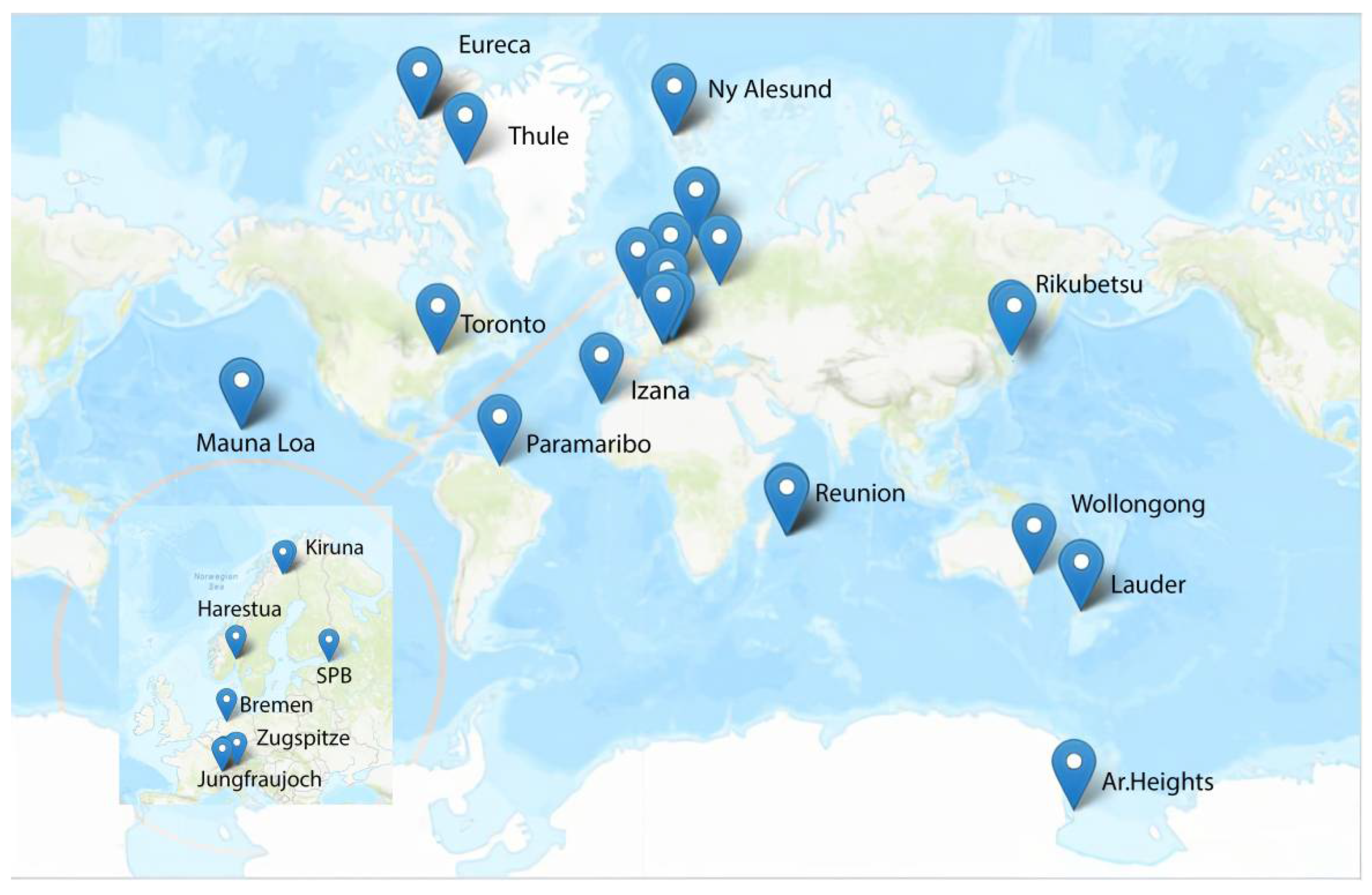
| № | Station | Latitude/Longitude, ° | Altitude, m a.s.l. | Sea Level Conversion Factor | Measur. Period | Measured Parameter |
|---|---|---|---|---|---|---|
| 1 | Eureka, Canada | 80.0N/86.4W | 610 | 0.926 | 2006–2020 | CH4/CO |
| 2 | Ny Ålesund, Norway | 78.9N/11.9E | 15 | 0.998 | 2003–2022 | CH4/CO |
| 3 | Thule, Greenland | 76.5N/68.7W | 220 * | 0.973 | 2003–2022 | CH4/CO |
| 4 | Kiruna, Sweden | 67.8N/20.4E | 419 | 0.949 | 2003–2022 | CH4/CO |
| 5 | Harestua, Norway | 60.2N/10.8E | 596 | 0.928 | 2009–2020 | CH4 |
| 2003–2018 | CO | |||||
| 6 | St. Petersburg, Russian Federation | 59.9N/29.8E | 20 | 0.997 | 2009–2022 | CH4/CO |
| 7 | Bremen, Germany | 53.1N/8.8E | 27 | 0.997 | 2003–2022 | CH4/CO |
| 8 | Zugspitze, Germany | 47.4N/11.0E | 2964 | 0.690 | 2003–2022 | CH4/CO |
| 9 | Jungfraujoch, Switzerland | 46.5N/8.0E | 3580 | 0.638 | 2003–2022 | CH4/CO |
| 10 | Toronto—TAO, Canada | 43.7N/79.4W | 174 | 0.978 | 2002–2019 ** | CH4 |
| 2003–2022 | CO | |||||
| 11 | Rikubetsu, Japan | 43.5N/143.8E | 380 | 0.953 | 2003–2019 | CH4 |
| 2003–2018 | CO | |||||
| 12 | Izaña, Tenerife, Spain | 28.3N/16.5W | 2367 | 0.743 | 2003–2022 | CH4/CO |
| 13 | Mauna Loa, HI, United States | 19.5N/155.9W | 3397 | 0.653 | 2003–2022 | CH4/CO |
| 14 | Paramaribo, Suriname | 5.7N/55.2W | 23 | 0.997 | 2004–2022 | CH4 |
| 2004–2018 | CO | |||||
| 15 | Reunion Island, Maido, France | 21.1S/55.4E | 2155 | 0.763 | 2013–2019 | CH4/CO |
| 16 | Wollongong, Australia | 34.4S/150.9E | 30 | 0.996 | 2003–2022 | CH4/CO |
| 17 | Lauder, New Zealand | 45.0S/169.7E | 370 | 0.955 | 2003–2021 | CH4/CO |
| 18 | Arrival Heights, Antarctica | 77.8S/166.7E | 184 | 0.977 | 2003–2022 | CH4/CO |
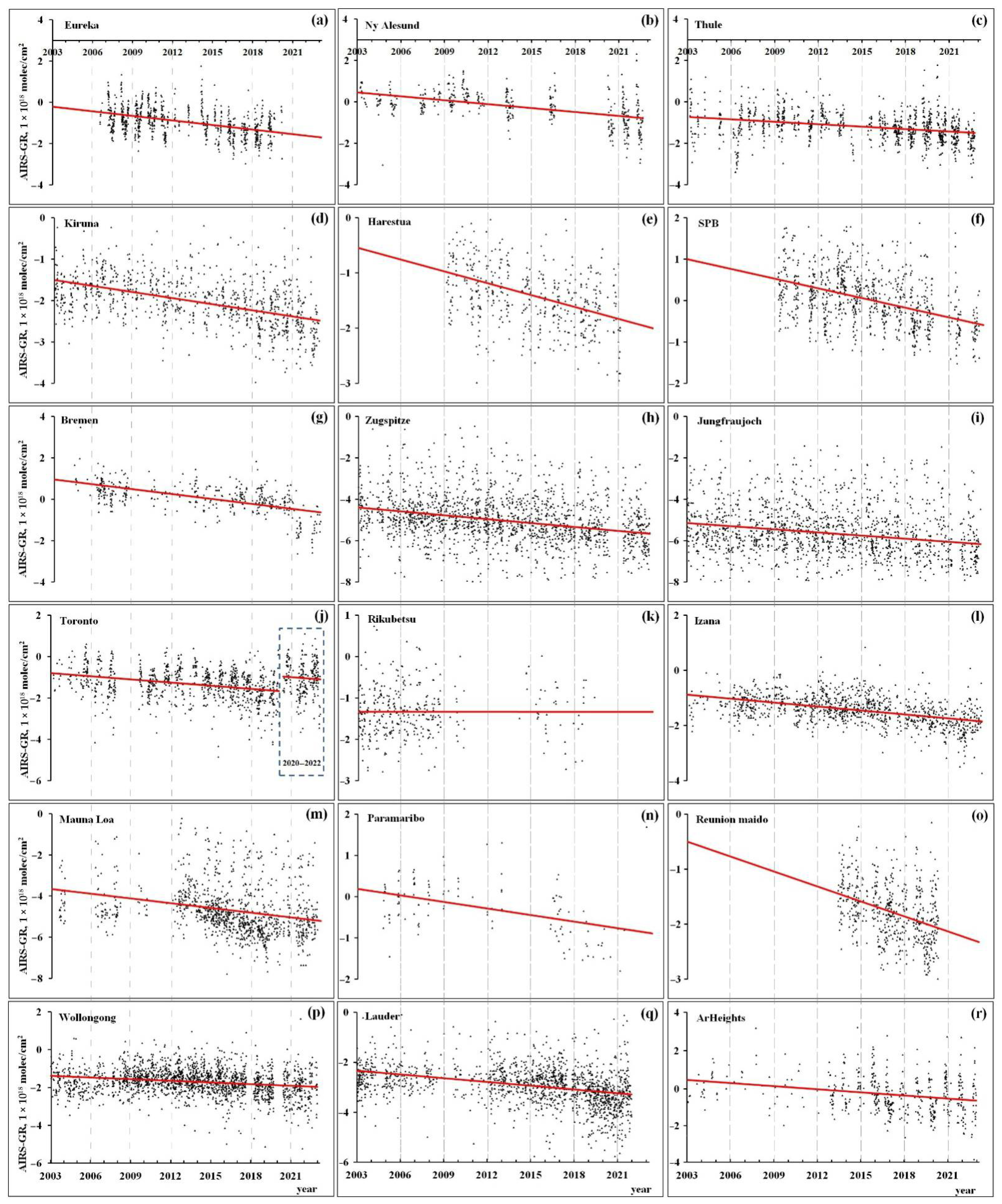
| No. | Monitoring Site | Slope of Difference Trend, Molecules/cm2 (×10)13 | Number of Synchronised Measurements (Pairs) |
|---|---|---|---|
| 1 | Eureka | −2.02 ± 2.86 | 810 |
| 2 | Ny Alesund | −1.82 ± 3.05 | 417 |
| 3 | Thule | −1.07 ± 2.02 | 1027 |
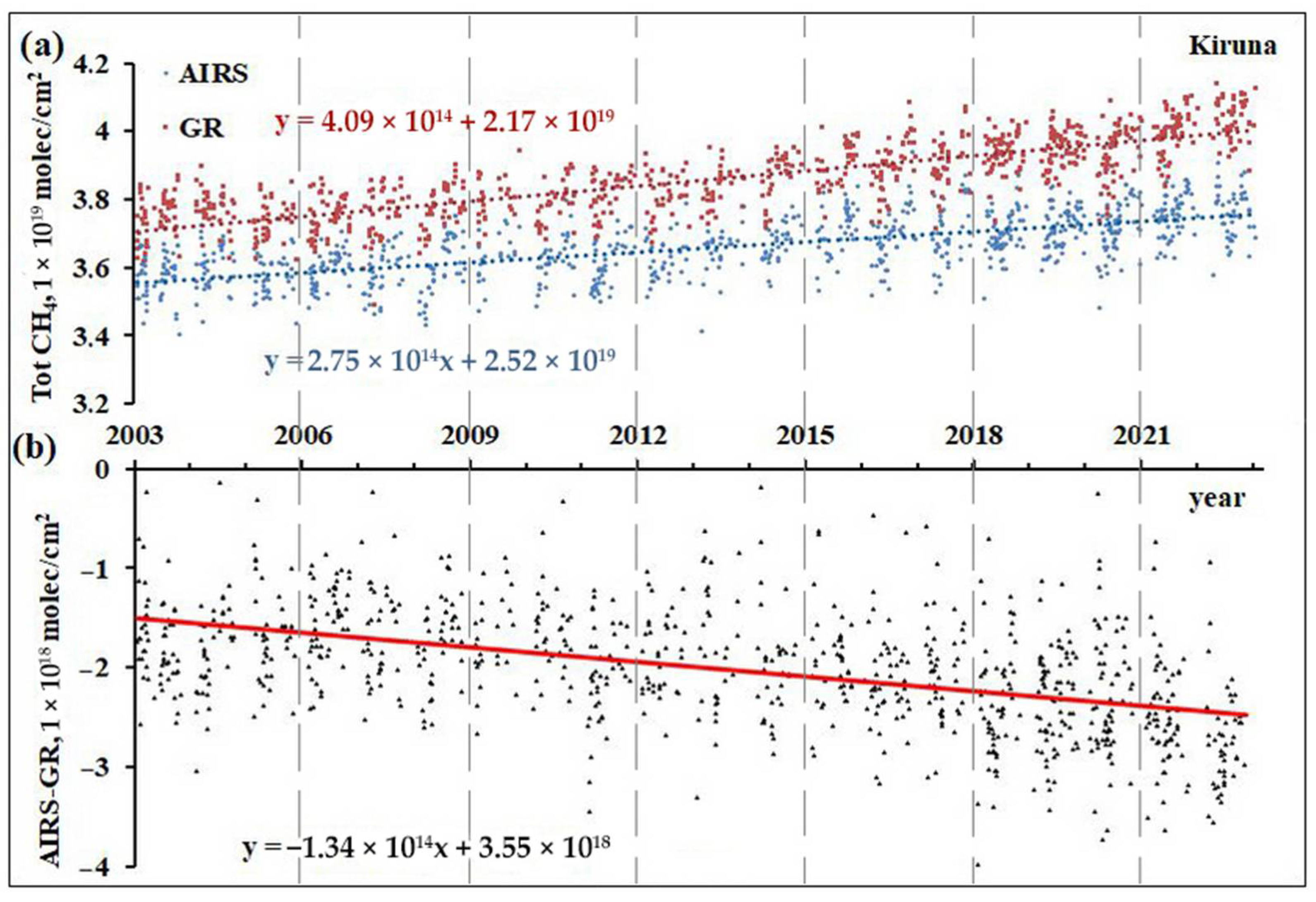
| 4 | Kiruna | −1.34 ± 1.54 | 907 |
| 5 | Harestua | −1.98 ± 4.50 | 462 |
| 6 | SPB | −2.18 ± 3.02 | 859 |
| 7 | Bremen | −2.42 ± 2.97 | 356 |
| 8 | Zugspitze | −1.75 ± 2.76 | 1721 |
| 9 | Jungfraujoch | −1.40 ± 3.27 | 1441 |
| 10 | Toronto | −1.43 ± 2.96 | 863 |
| 11 | Rikubetsu | ND * | 364 |
| 12 | Izana | −1.33 ± 1.48 | 1081 |
| 13 | Mauna Loa | −2.14 ± 4.63 | 1082 |
| 14 | Paramaribo | ND* | 122 |
| 15 | Reunion Maido | −2.54 ± 5.64 | 542 |
| 16 | Wollongong | −0.81 ± 1.67 | 1963 |
| 17 | Lauder | −1.37 ± 1.81 | 1578 |
| 18 | Arrival Heights | −1.49 ± 5.06 | 492 |
| Average | −1.69 ± 3.08 |
| No. | Monitoring Site | Original Data | Corrected Data | ||
|---|---|---|---|---|---|
| Correlation, R | Orthogonal Regression Equation | Correlation, R | Orthogonal Regression Equation | ||
| 1 | Eureka | 0.62 | 0.62x + 1.35 × 10¹⁹ | 0.72 | 0.83x + 6.00 × 10¹⁸ |
| 2 | Ny Alesund | 0.74 | 0.65x + 1.31 × 10¹⁹ | 0.82 | 0.97x + 1.74 × 10¹⁸ |
| 3 | Thule | 0.66 | 0.86x + 3.99 × 10¹⁸ | 0.76 | 1.22x − 8.74 × 10¹⁸ |
| 4 | Kiruna | 0.84 | 0.78x + 6.54 × 10¹⁸ | 0.90 | 1.07x − 4.07 × 10¹⁸ |
| 5 | Harestua | 0.58 | 1.20x − 1.22 × 10¹⁹ | 0.75 | 0.91x + 2.63 × 10¹⁸ |
| 6 | SPB | 0.69 | 0.85x + 5.70 × 10¹⁸ | 0.78 | 1.06x − 1.53 × 10¹⁸ |
| 7 | Bremen | 0.81 | 0.62x + 1.48 × 10¹⁹ | 0.88 | 0.89x + 4.97 × 10¹⁸ |
| 8 | Zugspitze | 0.48 | 1.32x − 1.74 × 10¹⁹ | 0.61 | 1.53x − 2.49 × 10¹⁹ |
| 9 | Jungfraujoch | 0.46 | 1.39x − 2.08 × 10¹⁹ | 0.58 | 1.61x − 2.85 × 10¹⁹ |
| 10 | Toronto | 0.58 | 0.56x + 1.61 × 10¹⁹ | 0.67 | 0.89x + 3.72 × 10¹⁸ |
| 11 | Rikubetsu | 0.61 | 1.24x − 1.03 × 10¹⁹ | 0.67 | 1.61x − 2.43 × 10¹⁹ |
| 12 | Izana | 0.83 | 0.81x + 6.15 × 10¹⁸ | 0.90 | 1.14x − 6.51 × 10¹⁸ |
| 13 | Mauna Loa | 0.36 | 2.02x − 4.57 × 10¹⁹ | 0.49 | 2.01x − 4.44 × 10¹⁹ |
| 14 | Paranaribo | 0.58 | 0.37x + 2.41 × 10¹⁹ | 0.68 | 0.76x + 9.40 × 10¹⁸ |
| 15 | Reunion Maido | 0.46 | 1.36x − 1.63 × 10¹⁹ | 0.59 | 1.52x − 2.16 × 10¹⁹ |
| 16 | Wollongong | 0.69 | 1.04x − 3.34 × 10¹⁸ | 0.78 | 1.38x − 1.53 × 10¹⁹ |
| 17 | Lauder | 0.65 | 1.08x − 6.05 × 10¹⁸ | 0.77 | 1.36x − 1.58 × 10¹⁹ |
| 18 | Arrival Heights | 0.38 | 1.29x − 1.04 × 10¹⁹ | 0.53 | 1.58x − 1.99 × 10¹⁹ |
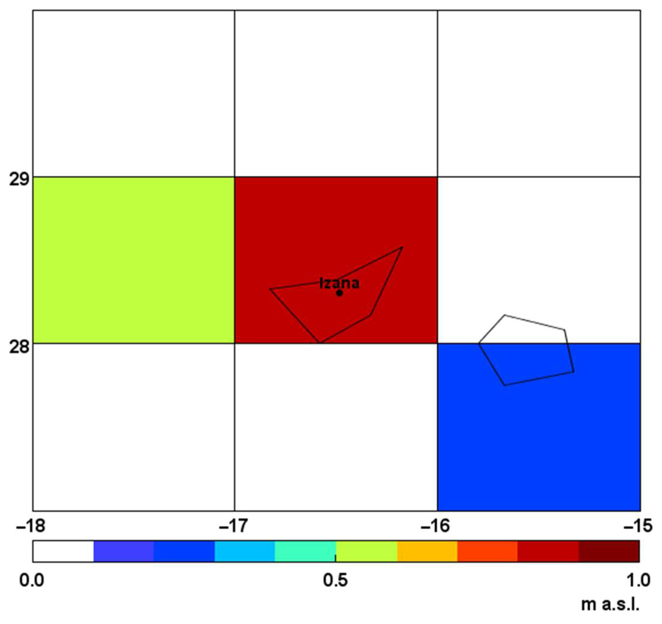
| No. | Monitoring Site | Actual Altitude, m a.s.l. | AIRS-Based Altitude, m a.s.l. |
|---|---|---|---|
| 1 | Zugspitze | 2964 | 1264 |
| 2 | Jungfraujoch | 3580 | 1551 |
| 3 | Izana | 2367 | 1 |
| 4 | Mauna Loa | 3397 | 1301 |
| 5 | Reunion Maido | 2155 | 0 |
| No. | Monitoring Site | Initial Trend, %/Year | Trend After Drift Correction, %/Year | |||
|---|---|---|---|---|---|---|
| AIRS | GR | Δ, AIRS-GR | AIRS | Δ, AIRS-GR | ||
| 1 | Eureka | 0.14 ± 0.03 | 0.33 ± 0.03 | −0.19 | 0.30 ± 0.03 | 0.03 |
| 2 | Ny Alesund | 0.27 ± 0.03 | 0.44 ± 0.03 | −0.17 | 0.42 ± 0.03 | 0.02 |
| 3 | Thule | 0.21 ± 0.02 | 0.31 ± 0.02 | −0.10 | 0.37 ± 0.02 | 0.06 |
| 4 | Kiruna | 0.27 ± 0.02 | 0.39 ± 0.02 | −0.11 | 0.43 ± 0.02 | 0.05 |
| 5 | Harestua | 0.25 ± 0.05 | 0.46 ± 0.05 | −0.21 | 0.44 ± 0.04 | −0.02 |
| 6 | SPB | 0.28 ± 0.03 | 0.48 ± 0.03 | −0.20 | 0.43 ± 0.03 | −0.05 |
| 7 | Bremen | 0.30 ± 0.03 | 0.53 ± 0.03 | −0.23 | 0.46 ± 0.03 | −0.07 |
| 8 | Zugspitze | 0.29 ± 0.03 | 0.42 ± 0.01 | −0.13 | 0.47 ± 0.03 | 0.05 |
| 9 | Jungfraujoch | 0.33 ± 0.03 | 0.41 ± 0.02 | −0.08 | 0.51 ± 0.03 | 0.10 |
| 10 | Toronto | 0.24 ± 0.02 | 0.37 ± 0.03 | −0.12 | 0.40 ± 0.02 | 0.03 |
| 11 | Rikubetsu | 0.27 ± 0.04 | 0.26 ± 0.03 | 0.01 | 0.43 ± 0.04 | 0.18 |
| 12 | Izana | 0.32 ± 0.01 | 0.43 ± 0.01 | −0.11 | 0.48 ± 0.01 | 0.04 |
| 13 | Mauna Loa | 0.30 ± 0.05 | 0.46 ± 0.02 | −0.16 | 0.46 ± 0.04 | 0.01 |
| 14 | Paranaribo | 0.20 ± 0.03 | 0.35 ± 0.06 | −0.15 | 0.35 ± 0.03 | 0 |
| 15 | Reunion Maido | 0.28 ± 0.05 | 0.50 ± 0.02 | −0.22 | 0.44 ± 0.05 | −0.06 |
| 16 | Wollongong | 0.33 ± 0.02 | 0.39 ± 0.01 | −0.06 | 0.49 ± 0.02 | 0.10 |
| 17 | Lauder | 0.24 ± 0.02 | 0.36 ± 0.01 | −0.11 | 0.41 ± 0.02 | 0.06 |
| 18 | Arrival Heights | 0.25 ± 0.05 | 0.40 ± 0.03 | −0.15 | 0.41 ± 0.05 | 0.01 |
| Average | 0.26 ± 0.03 | 0.40 ± 0.02 | 0.43 ± 0.03 | |||
| No. | Monitoring Site | Slope of Difference, Molecules/cm2 (×10)12 | R | AIRS Trend, %/Year | GR Trend, %/Year | Δ, AIRS-GR | Number of Compared Pairs |
|---|---|---|---|---|---|---|---|
| 1 | Eureka | 36.8 ± 8.20 | 0.80 | −0.13 ± 0.18 | −0.84 ± 0.26 | 0.70 | 777 |
| 2 | NY Alesund | 19.2 ± 5.61 | 0.95 | −0.79 ± 0.24 | −1.15 ± 0.30 | 0.36 | 415 |
| 3 | Thule | 30.3 ± 3.28 | 0.93 | −0.60 ± 0.10 | −1.15 ± 0.14 | 0.54 | 1315 |
| 4 | Kiruna | 10.1 ± 3.72 | 0.92 | −0.80 ± 0.14 | −0.93 ± 0.16 | 0.13 | 752 |
| 5 | Harestua | 13.8 ± 5.39 | 0.91 | −1.19 ± 0.20 | −1.37 ± 0.21 | 0.18 | 681 |
| 6 | SPB | −4.89 ± 5.25 | 0.93 | −0.89 ± 0.25 | −0.80 ± 0.26 | 0.10 | 793 |
| 7 | Bremen | −1.33 ± 6.12 | 0.90 | −0.98 ± 0.23 | −0.93 ± 0.22 | 0.05 | 428 |
| 8 | Zugspitse | −5.59 ± 1.99 | 0.91 | −0.78 ± 0.10 | −0.61 ± 0.09 | 0.17 | 2137 |
| 9 | Jungfrau | −10.9 ± 2.78 | 0.92 | −1.11 ± 0.15 | −0.82 ± 0.14 | 0.29 | 1219 |
| 10 | Toronto | −3.93 ± 4.45 | 0.85 | −0.87 ± 0.14 | −0.76 ± 0.14 | 0.11 | 1479 |
| 11 | Rikubetsu | −5.17 ± 11.2 | 0.93 | −1.40 ± 0.42 | −1.21 ± 0.43 | 0.19 | 352 |
| 12 | Izana | −1.88 ± 3.16 | 0.88 | −0.45 ± 0.13 | −0.43 ± 0.13 | 0.01 | 1154 |
| 13 | Mauna Loa | −8.64 ± 7.18 | 0.85 | −0.95 ± 0.26 | −0.73 ± 0.30 | 0.23 | 1278 |
| 14 | Paramaribo | −8.14 ± 11.1 | 0.87 | −0.89 ± 0.39 | −0.71 ± 0.37 | 0.17 | 175 |
| 15 | Reunion maido | 0.76 ± 8.95 | 0.94 | 1.27 ± 0.59 | 1.23 ± 0.62 | 0.04 | 818 |
| 16 | Wollongong | 6.28 ± 3.80 | 0.79 | −0.33 ± 0.13 | −0.48 ± 0.16 | 0.15 | 2579 |
| 17 | Lauder | −7.81 ± 1.96 | 0.89 | −0.03 ± 0.13 | 0.22 ± 0.14 | 0.25 | 1695 |
| 18 | Arrival Heights | −14.2 ± 3.22 | 0.90 | −0.28 ± 0.26 | 0.24 ± 0.31 | 0.52 | 483 |
| Average | −0.62 ± 0.22 | −0.62 ± 0.24 |
Disclaimer/Publisher’s Note: The statements, opinions and data contained in all publications are solely those of the individual author(s) and contributor(s) and not of MDPI and/or the editor(s). MDPI and/or the editor(s) disclaim responsibility for any injury to people or property resulting from any ideas, methods, instructions or products referred to in the content. |
© 2025 by the authors. Licensee MDPI, Basel, Switzerland. This article is an open access article distributed under the terms and conditions of the Creative Commons Attribution (CC BY) license (https://creativecommons.org/licenses/by/4.0/).
Share and Cite
Rakitin, V.; Fedorova, E.; Skorokhod, A.; Kirillova, N.; Pankratova, N.; Elansky, N. Principles of Correction for Long-Term Orbital Observations of Atmospheric Composition, Applied to AIRS v.6 CH4 and CO Data. Remote Sens. 2025, 17, 2323. https://doi.org/10.3390/rs17132323
Rakitin V, Fedorova E, Skorokhod A, Kirillova N, Pankratova N, Elansky N. Principles of Correction for Long-Term Orbital Observations of Atmospheric Composition, Applied to AIRS v.6 CH4 and CO Data. Remote Sensing. 2025; 17(13):2323. https://doi.org/10.3390/rs17132323
Chicago/Turabian StyleRakitin, Vadim, Eugenia Fedorova, Andrey Skorokhod, Natalia Kirillova, Natalia Pankratova, and Nikolai Elansky. 2025. "Principles of Correction for Long-Term Orbital Observations of Atmospheric Composition, Applied to AIRS v.6 CH4 and CO Data" Remote Sensing 17, no. 13: 2323. https://doi.org/10.3390/rs17132323
APA StyleRakitin, V., Fedorova, E., Skorokhod, A., Kirillova, N., Pankratova, N., & Elansky, N. (2025). Principles of Correction for Long-Term Orbital Observations of Atmospheric Composition, Applied to AIRS v.6 CH4 and CO Data. Remote Sensing, 17(13), 2323. https://doi.org/10.3390/rs17132323