Abstract
While space weather indices (e.g., F10.7, Dst index) are commonly employed to characterize ionospheric activity levels, the Global Mean Electron Content (GMEC) provides a more direct and comprehensive indicator of the global ionospheric state. This metric demonstrates greater potential than space weather indices for calibrating empirical ionospheric models such as IRI-2020. The COSMIC-2 constellation enables continuous, all-weather global ionospheric monitoring via radio occultation, unimpeded by land–sea distribution constraints, with over 8000 daily occultation events suitable for GMEC modeling. This study developed two lightweight GMEC models using COSMIC-2 data: (1) a POD GMEC model based on slant TEC (STEC) extracted from Level 1b podTc2 products and (2) a PROF GMEC model derived from vertical TEC (VTEC) calculated from electron density profiles (EDPs) in Level 2 ionPrf products. Both backpropagation neural network (BPNN)-based models generate hourly GMEC outputs as global spatial averages. Critically, GMEC serves as an essential intermediate step that addresses the challenges of utilizing spatially irregular occultation data by compressing COSMIC-2’s ionospheric information into an integrated metric. Building on this compressed representation, we implemented a convolutional neural network (CNN) that incorporates GMEC as an auxiliary feature to calibrate IRI-2020’s global ionospheric maps. This approach enables computationally efficient correction of systemic IRI TEC errors. Experimental results demonstrate (i) 48.5% higher accuracy in POD/PROF GMEC relative to IRI-2020 GMEC estimates, and (ii) the calibrated global IRI TEC model (designated GCIRI TEC) reduces errors by 50.15% during geomagnetically quiet periods and 28.5% during geomagnetic storms compared to the original IRI model.
1. Introduction
The ionosphere is a key region of the Sun–Earth space environment and serves as a critical interface for energy exchange between the Earth’s atmosphere and outer space. It also plays a significant role in the propagation and performance of radio signals and communication systems. Monitoring the ionosphere is essential for revealing the coupling mechanisms of the Sun–Earth system and mitigating the impacts of space weather phenomena, such as solar flares and coronal mass ejections. This process provides critical support for safeguarding the accuracy of satellite navigation systems and the reliability of communication infrastructures [1].
Various parameters are used to characterize ionospheric activity, which can be broadly classified into two categories. The first includes indices related to external drivers of the ionosphere, such as the F10.7 index, sunspot numbers (SSNs), Kp index, and Disturbance Storm Time index (Dst). As the ionosphere is influenced by both solar and geomagnetic activity, the total electron content (TEC) of the ionosphere often shows strong correlations with these space weather indicators. The second category includes parameters that directly describe the physical state of the ionosphere, such as peak electron density and TEC. In particular, vertical TEC refers to the integral of electron density along the vertical column from the bottom to the top of the ionosphere [2]. TEC monitoring plays a vital role in correcting satellite navigation errors and in characterizing ionospheric disturbances in near-Earth space.
The Global Mean Electron Content (GMEC) represents a weighted average of the TEC across the entire ionosphere. By averaging TEC values on a global scale, GMEC effectively suppresses local ionospheric variations and highlights the overall characteristics of the ionosphere. As a result, it serves as a more suitable metric than regional TEC for studying long-term global ionospheric trends [3]. Since GMEC directly reflects the intensity of global ionospheric activity, it offers a more representative measure of the ionospheric state than traditional solar and geomagnetic indices. However, unlike other indices of solar–terrestrial activity (such as Dst index and SSN), GMEC cannot be directly observed. It must be calculated using global ionospheric models, such as the global ionospheric maps released by IGS ionosphere associate analysis centers (IAACs) [4].
The development of radio occultation (RO) technology has provided new opportunities for ionospheric monitoring. GNSS-based radio occultation leverages dual-frequency receivers onboard low Earth orbit (LEO) satellites, such as COSMIC-2 mission, to capture GNSS signals as they are occulted by the Earth’s atmosphere. By analyzing changes in the refractive index along the signal propagation path, atmospheric parameters can be retrieved [5,6]. RO technology offers several key advantages, including all-weather capability, global coverage, high vertical resolution, and near-real-time capabilities, making it particularly effective in compensating for the lack of ionospheric observation data in specific regions, such as over oceans, thereby enabling the acquisition of global ionospheric data [7].
Although RO has already demonstrated significant success in ionospheric electron density profiling and global ionospheric map construction, no prior research has explored its application in constructing a Global Mean Electron Content model. Given its immunity to tropospheric effects and ground infrastructure constraints, as well as its global coverage and fine vertical resolution, radio occultation provides a promising alternative for developing a robust and independent GMEC model, potentially overcoming the limitations of traditional ground-based methods.
Compared to existing global ionospheric map (GIM)-derived GMEC products (e.g., from CODE/IGS), the COSMIC-2-based GMEC demonstrates significant advantages: (1) Infrastructure: the former requires hundreds of globally distributed GNSS ground stations and communication links, whereas the latter relies solely on a limited constellation of occultation satellites and satellite-to-ground communication technology. (2) Processing complexity: the former depends on complex global ionospheric modeling workflows, while the latter holds the potential for a lightweight GMEC indicator model. (3) Spatial coverage: the former exhibits data voids over oceanic regions, whereas the latter achieves uniform observational coverage across both oceanic and terrestrial domains. Notably, COSMIC-2 observations are confined to low and mid-latitudes, warranting investigation into whether this limited spatial coverage sufficiently characterizes global ionospheric variability.
Due to the heterogeneous nature of radio occultation observations—including slant TEC (STEC) along satellite ray paths and retrieved vertical electron density profiles—it is challenging to establish a nonlinear relationship with global GMEC using traditional mathematical approaches such as linear regression. Machine learning (ML) techniques, with their inherent capability to model complex nonlinear relationships, offer a promising solution for this task [8,9,10]. As such, ML methods are adopted in this study to construct the GMEC model. On the other hand, space weather parameters—including GMEC—play a critical role in monitoring ionospheric variability and updating ionospheric models. Previous studies have demonstrated that incorporating solar and geomagnetic activity indices into ionospheric modeling can significantly enhance model accuracy [11,12,13,14]. For instance, Liu et al. [9] proposed an LSTM-based ionospheric forecasting model augmented with solar extreme ultraviolet (EUV) and Dst indices, achieving a prediction accuracy of 1.27 TECU during geomagnetic storms and 0.86 TECU during quiet periods. Gao et al. [14] developed a convolutional LSTM model that refines IRI-derived TEC values using F10.7, SSN, Dst, and Kp indices as additional input channels, resulting in a 40.8% accuracy improvement during years of high solar activity. Since GMEC more directly reflects the global ionospheric state compared to other space weather indices, integrating RO-based GMEC into empirical ionospheric models for global TEC correction holds great potential for significantly improving model performance.
In this study, we propose an equivalent global mean TEC model based on a backpropagation neural network (BPNN), which uses COSMIC-2 occultation data and the solar activity index F10.7 as inputs. The accuracy of the global mean TEC model and its response to geomagnetic storms are validated. Furthermore, we introduce a convolutional neural network (CNN) that incorporates global mean TEC as an additional feature to refine the IRI-2020 global TEC model, in order to assess the calibration capability of GMEC for empirical global ionospheric TEC models.
2. Materials and Methods
2.1. COSMIC-2 Data
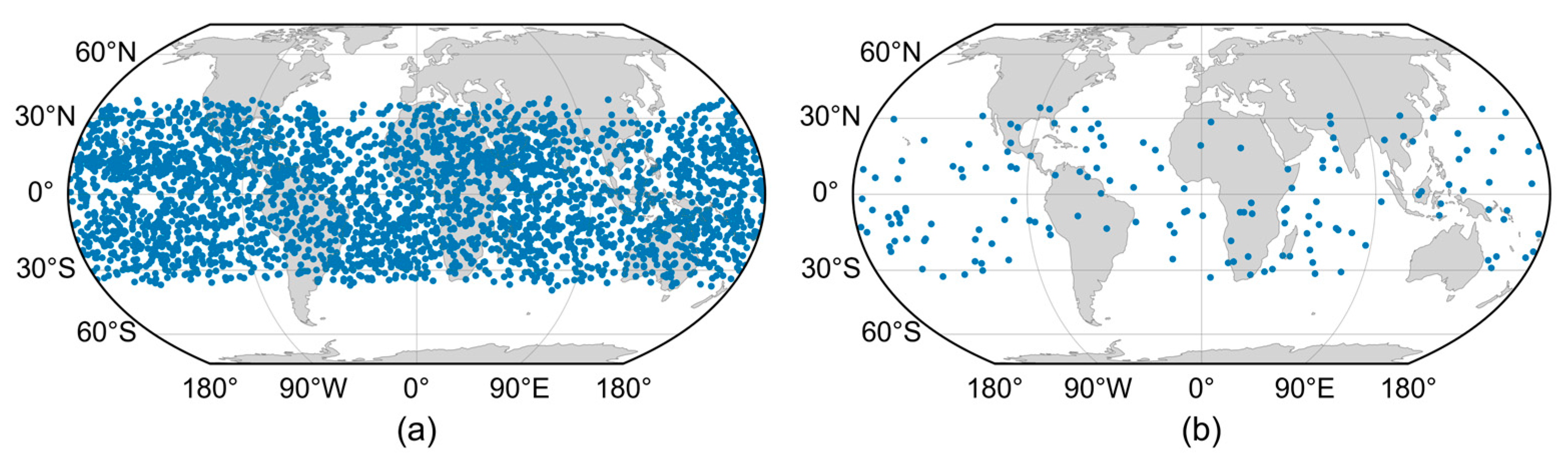
COSMIC-2 is a satellite system developed through a collaboration between the National Space Organization of Taiwan (NSPO) and the National Oceanic and Atmospheric Administration (NOAA) of the United States. The system was successfully launched in June 2019, replacing the retired COSMIC-1 satellites [6]. This constellation consists of six satellites equipped with next-generation GNSS Radio Occultation payloads, with an orbital inclination of 24 degrees and an altitude of approximately 550 km [15]. Figure 1 illustrates the concept of GNSS-RO. GNSS-RO refers to the process in which the relative motion between a LEO satellite and a GNSS satellite causes the signal path to cut into or out of the edge of the atmosphere [16]. The near-horizontal incident angle of the signal provides GNSS-RO with rich horizontal stratification information. The raw data from COSMIC-2 are processed by the data processing center operated by the University Corporation for Atmospheric Research (UCAR). The data sources used in this study include the Level 2 ionPrf product and the Level 1b podTc2 product from COSMIC-2. The ionPrf product provides electron density profile data derived using the Abel inversion algorithm. Given that the ionPrf inversion assumes spherical symmetry and neglects errors caused by the drift of the occultation point during the occultation event, a comparative model using the lower-level Level 1b podTc2 product as input was also designed. The podTc2 product provides absolute TEC data along the ray path at the time of the occultation event (see Table 1). The COSMIC-2 mission delivers more than 8000 radio occultation events daily. Figure 2 shows the global distribution of occultation events from COSMIC-2 within a 1-day and 1 h time frame. As seen, the occultation events provide coverage over global mid- and low-latitude regions, offering an advantage over ground-based GNSS networks, which are typically limited to land-based distributions.
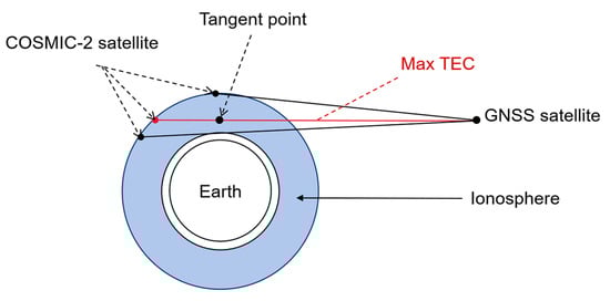
Figure 1.
COSMIC-2 ionospheric radio occultation observations.

Table 1.
Selected input features for the two types of data from COSMIC-2.

Figure 2.
Global distribution of occultation events: (a) full day of 1 February 2024; (b) from 7:00 to 8:00 a.m. on 2 February 2024.
For the two data sources, different input features were selected to represent the information contained in each radio occultation event (see Table 1). For the ionPrf product, the model input features include the location of the occultation event (longitude, latitude) and the VTEC obtained by integrating the electron density profile data. For the podTc2 product, due to the spatial inhomogeneity of the ionosphere, both the location of the tangent point and the azimuth angle of the ray’s incidence affect the TEC along the ray path. To account for the differences between occultation events, the model uses the maximum TEC value of each occultation event, the location of the tangent point location (latitude and longitude), and the azimuth angle of the LEO satellite as the data features for each event (see Figure 1 and Figure 3). The maximum TEC value during each radio occultation event typically occurs within the tangent point altitude range of approximately 250 to 400 km, which corresponds to the region where the TEC density in the ionosphere is predominantly concentrated.
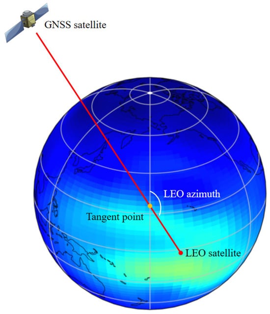
Figure 3.
The influence of occultation tangent point location and incidence azimuth angle on the STEC of radio occultation observations.
2.2. F10.7
F10.7 represents the solar radio flux at a wavelength of 10.7 cm. It effectively reflects the influence of solar activity on the plasma density in the upper atmosphere and ionosphere, making it a key parameter for studying the relationship between solar activity and Earth’s ionosphere [17].
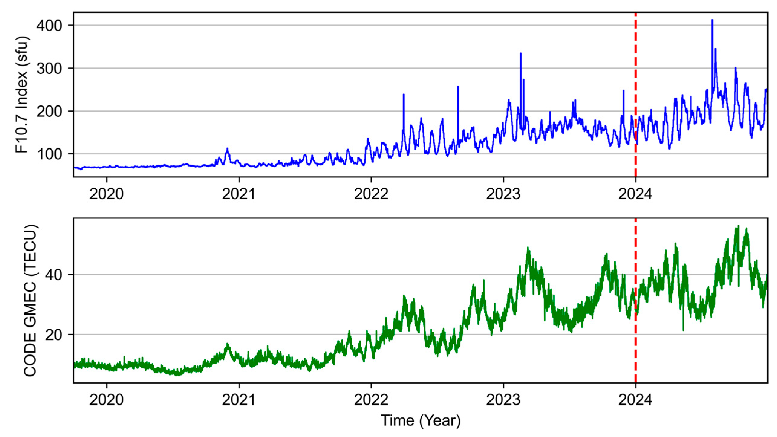
To account for the impact of solar activity on the ionosphere, F10.7 is used as an additional feature in the GMEC model. Figure 4 shows the time series of the F10.7 index during the experiment. It is evident that there is a certain correlation between the global mean TEC and variations in solar activity. In the figure, the red dashed line (31 December 2023) marks the boundary where data before this date were used for model training and validation, while the data after this date were used for model testing. As the 25th solar cycle began in December 2019, during the experiment, both the GMEC and the F10.7 index generally exhibited similar upward trends, reaching a peak in 2024. Intense solar activity presents significant challenges in ionospheric parameter modeling.
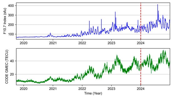
Figure 4.
Time series of F10.7 (top) and GMEC (bottom) during the experiment. Data before the red dashed line (31 December 2023) were used for training and validation, while data after the red dashed line were used for testing. The GMEC is calculated based on CODE GIM.
2.3. CODE GIM
The GIM provided by the Center for Orbit Determination in Europe (CODE) are gridded TEC maps represented by spherical harmonics (SHs) based on GNSS measurements from global ground stations [18]. The GIM data are provided in the Ionospheric Map Exchange (IONEX) format, with a spatial resolution of 5° (longitude) × 2.5° (latitude), meaning that each time step contains 5183 VTEC grid points (71 × 73) [19]. Since 19 October 2014, the temporal resolution of the CODE GIM has been updated from the original 2 h to 1 h [19]. In this study, we used CODE GIM data covering the period from 1 October 2019, to 31 December 2024, and computed the corresponding Global Mean Electron Content (GMEC) for each hour, which served as the output for training the equivalent GMEC model.
The formula for calculating GMEC based on the CODE ionospheric grid is as follows [20]:
where represents the TEC at the CODE grid point (i,j), denotes the geographic latitude of the grid point, and and are the differences in longitude and latitude directions for the spherical rectangle. represents the Earth’s average radius, taken as 6371 km in this study.
2.4. International Reference Ionosphere 2020 Model (IRI-2020)
The International Reference Ionosphere (IRI) model, developed by the Committee on Space Research (COSPAR) and the International Union of Radio Science (URSI), serves as the international standard for specifying Earth’s ionospheric parameters [21]. The IRI model describes the monthly average values of electron and ion densities as well as temperatures in the altitude range from 50 km to 2000 km, and provides VTEC from the lower boundary (60–80 km) to the user-specified upper boundary [22]. The latest version of the model is IRI-2020 [23].
Using the IRI-2020 model, global TEC distribution maps were calculated with a resolution consistent with that of the CODE GIM. The temporal resolution is 1 h, and the spatial resolution is 5° (longitude) × 2.5° (latitude).
2.5. Dataset Division
Using the ionPrf and podTc2 data products provided by the COSMIC-2 satellite, along with the F10.7 solar activity index, a feature set was constructed. The dataset covers the period from 1 October 2019, to 31 December 2024. The data are divided into 1 h intervals, with data from the half-hour before and after each hour’s timestamp forming a sample feature set. Within each time window, the GMEC value for the corresponding period is used as the target label, thereby constructing the sample dataset.
To ensure the accuracy and reliability of model evaluation, the data are divided into training, validation, and test sets based on time intervals. Specifically, data from 1 October 2019, to 31 December 2023, are used as the training and validation set, with an 8:2 ratio between the two. Data from 2024 serve as the test set, ensuring that the test set is completely independent of the training and validation sets and includes geomagnetic storm events, which allow for testing the model’s performance under extreme conditions. The training set is used to optimize and update model parameters via gradient descent to fit the model; the validation set is used to assess model performance, ensuring that overfitting or underfitting does not occur; the test set is then used to evaluate the model’s generalization ability when processing new, unseen data. Based on this division, a total of 34,942, 3883, and 9150 data samples were obtained for training, validation, and testing, respectively.
2.6. GMEC Model Construction
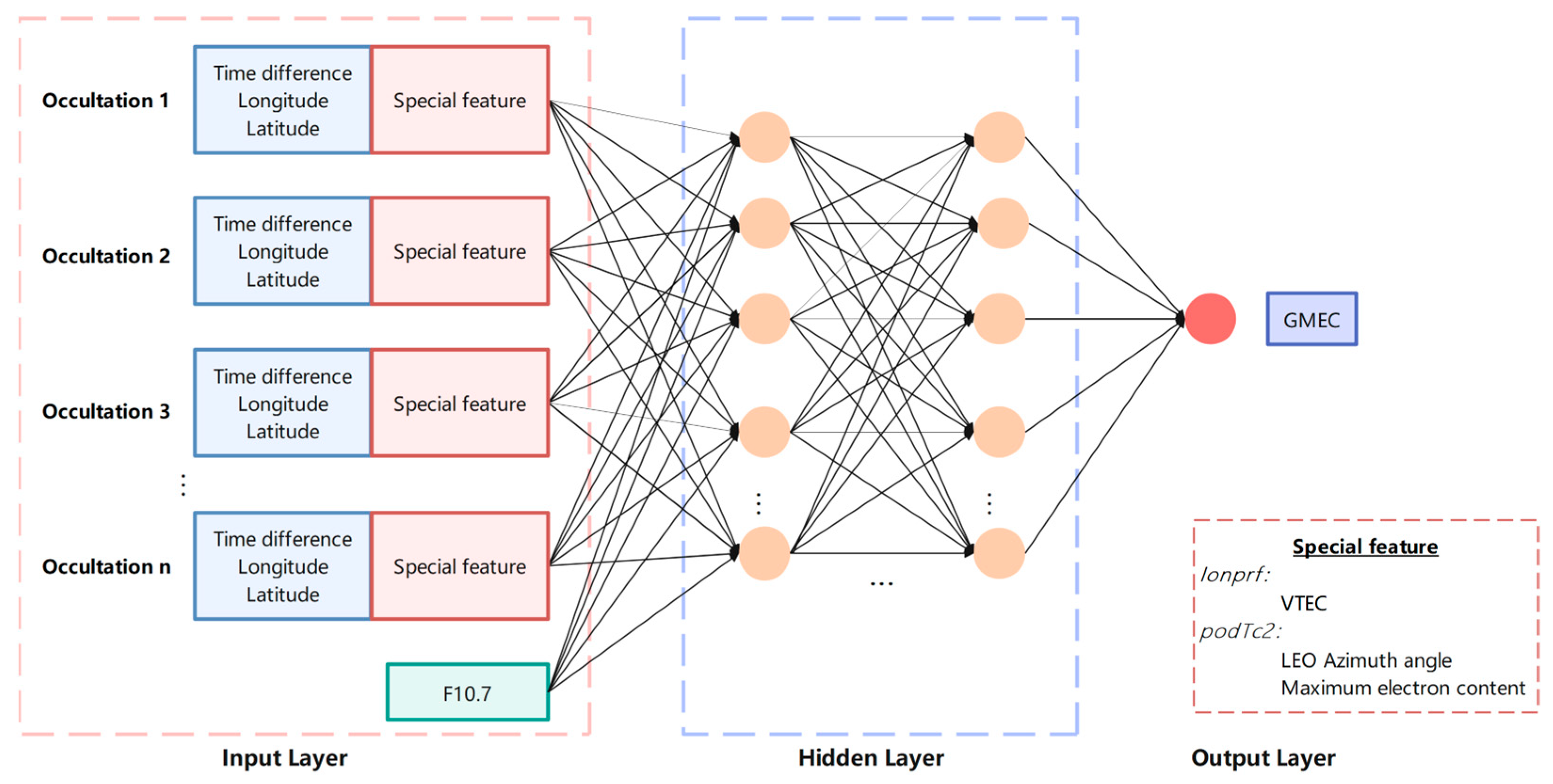
The backpropagation neural network (BPNN) is an artificial neural network based on a multilayer perceptron (MLP) architecture, widely used for regression and classification tasks. It consists of an input layer, multiple hidden layers, and an output layer, where the neurons in each layer are connected through weighted sums and undergo nonlinear transformations via an activation function. The BPNN computes outputs through forwardpropagation and adjusts the network’s weights through backpropagation. During backpropagation, the gradient of the loss function with respect to the network parameters is calculated using gradient descent, and the weights are updated according to the gradient to minimize the error. The advantage of BPNN lies in its ability to learn complex nonlinear relationships through the hidden layers, making it suitable for handling highly complex tasks.
Although there is a significant relationship between the VTEC data provided by the ionPrf product and the maximum electron content values provided by the podTc2 product, and the global mean TEC (GMEC), this relationship is complex and nonlinear, making it difficult to model accurately using precise mathematical or physical equations. Therefore, we utilize a BPNN model to predict the GMEC. Figure 5 illustrates the structure of the BPNN.
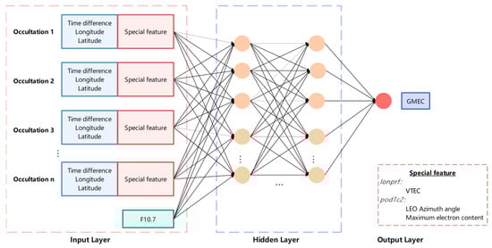
Figure 5.
Structure of the BPNN model for global mean TEC (GMEC).
Two approaches were designed for modeling GMEC (see Table 2). The PROF solution uses the VTEC obtained by vertically integrating the ionPrf electron density profile product, along with related features, as input features. In contrast, the POD solution uses the maximum electron content from the podTc2 product, along with related features, as input features. The final output is the predicted value of global mean TEC (GMEC). Table 2 provides a detailed description of the processing strategies for both approaches. For input parameters with different time resolutions, the data were resampled at 1 h intervals, consistent with the time resolution used by the GIM TEC product. To ensure the continuity of angular parameter inputs, such as longitude, latitude, and azimuth angle, all angular data were converted into sine and cosine components:
where represents angular variables such as longitude, latitude, and azimuth angle, and and are the transformed input features.
Table 2.
BPNN-based GMEC modeling schemes.
Furthermore, to ensure data dimensionality alignment, the number of occultation events for each time period is set to the maximum number of occultation events. When the actual number of occultation events is fewer than the maximum, the remaining observations are padded with zeros, and a label feature (0 or 1) is added to denote valid or invalid observations.
The input data dimensions for the PROF model are N × K1, where N represents the maximum number of occultation events and K1 is the number of input features, including VTEC, the time difference between the occultation event and the GMEC reference time, the sine and cosine components of the longitude and latitude of the occultation event, and the valid observation label.
The input data dimensions for the POD model are N × K2, where N represents the maximum number of occultation events and K2 is the number of input features, including MAX TEC; the time difference between the occultation event and the GMEC reference time; the sine and cosine components of the longitude, latitude, and azimuth angle of the LEO satellite; and the valid observation label.
The design of the BPNN model includes five hidden layers, each with a size of 64 neurons, and employs the Rectified Linear Unit (ReLU) activation function to introduce non-linearity. The output layer has a size of 1, corresponding to the predicted value of the Global Mean Electron Content (GMEC). During the training process, the mean squared error (MSE) is used as the loss function. The Adam optimizer is chosen, with the learning rate set to 0.001. The Adam optimizer features an adaptive learning rate, which dynamically adjusts the learning rate based on the gradient of each parameter, accelerating the model’s convergence and improving training stability. To prevent overfitting, an early stopping strategy is implemented. Specifically, training is halted early if the validation loss does not improve for 10 consecutive epochs, thus avoiding excessive fitting to the training data. During training, the loss for each epoch is computed and output in real-time, including both training and validation losses, to monitor the model’s performance. The test set is used for the final evaluation of the model’s performance, with the test loss and root mean square error (RMSE) calculated to further verify the accuracy of the model’s predictions.
2.7. GMEC-Based Calibration of the IRI-2020 Model
Related studies have shown that solar and geomagnetic activity indices can be used for ionospheric TEC modeling to improve model accuracy. Compared to indirect indicators of ionospheric activity such as F10.7, SSN, and Dst, GMEC more directly represents the overall level of global ionospheric activity. Based on this, we propose a method to calibrate the IRI-2020 GIM using the GMEC model constructed from COSMIC-2 data. Figure 6 illustrates the structure of the CNN architecture.
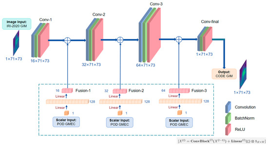
Figure 6.
Convolutional neural network (CNN) architecture incorporating GMEC as an additional feature.
The model is constructed using an artificial neural network. It takes the IRI-2020 GIM and the corresponding GMEC at each time step as inputs, and outputs the calibrated GIM product for the same time. To extract features from the input data, a convolutional neural network (CNN) is employed to process the IRI-2020 GIM, while the GMEC is incorporated as an additional feature and fused with the extracted representations for enhanced modeling.
The designed neural network accepts two types of input: one is the global ionospheric grid map from IRI-2020 with a spatial dimension of 71 × 73, and the other is the scalar GMEC predicted by the POD model. The output of the network is a 71 × 73 global ionospheric map corresponding to the CODE GIM. For dataset partitioning, the period from 1 October 2019, to 31 December 2023, is used for training and validation, with an 8:2 split. The data from 2024 is reserved for testing.
For the image input , convolutional layers are employed to extract spatial features. Assuming the input image has dimensions , where and denote the height and width, respectively, and is the number of channels, the convolutional operation can be expressed as
Here, represents the convolutional kernel, is the bias term, and is the resulting feature map. After multiple convolutional layers, the output feature map has dimensions , where is the number of output channels.
For the scalar input , a fully connected (dense) layer is used to transform the data, defined as
In this expression, and are the weights and bias of the fully connected layer, and is the output feature representation of the scalar input.
After extracting features from both input sources, feature fusion is performed at an intermediate stage of the network. Specifically, we adopt an element-wise addition strategy to combine the image and scalar features:
This fusion method involves broadcasting the scalar-derived feature map to match the spatial dimensions of the image feature map, thereby enabling both data types to jointly influence subsequent convolutional layers. The fused feature map is then passed through a final convolutional layer to produce the output prediction :
where and are the weights and bias of the final convolutional layer.
During training, the model uses mean squared error (MSE) as the loss function and applies the ReLU activation function throughout the network. The Adam optimizer—an adaptive optimization algorithm—was employed with an initial learning rate of 0.001. A batch size of 32 was used. To ensure optimal performance, the model with the lowest validation loss was selected and retained.
2.8. Model Evaluation
To quantitatively assess the predictive performance of the proposed model, we employed the following standard evaluation metrics: the root mean square error (RMSE), the mean absolute error (MAE), and Pearson correlation coefficient (R). These metrics measure the discrepancy between the model predictions and the corresponding ground truth values and are defined as follows:
where denotes the total number of samples, represents the model-predicted values, and denotes the corresponding ground truth values.
3. Results
3.1. GMEC Accuracy Validation
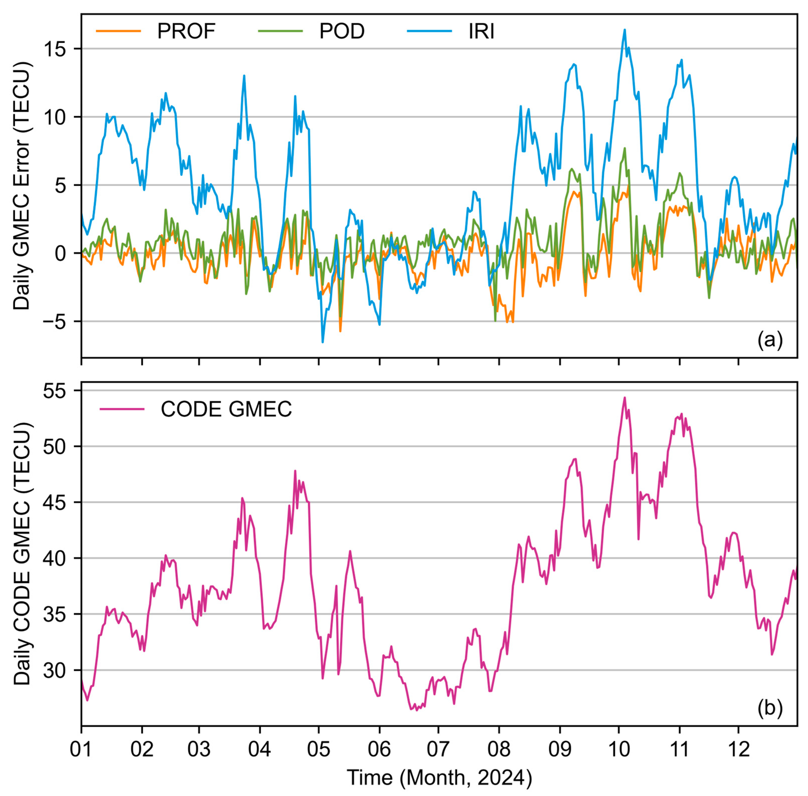
Both the Global Mean Electron Content derived from podTc2 data (POD GMEC) and the Global Mean Electron Content derived from ionPrf data (PROF GMEC) demonstrate significantly improved accuracy compared to the GMEC derived from the IRI-2020 model. Figure 7a presents the daily mean error time series for the 2024 test dataset, where CODE GMEC is used as the reference, and the error profiles of POD GMEC, PROF GMEC, and IRI-derived GMEC (IRI GMEC) are compared. Figure 7b shows the daily mean time series of CODE GMEC in 2024. As shown in the figure, the IRI GMEC error exhibits pronounced high-frequency and large-amplitude fluctuations throughout the test period, and the fluctuation amplitude shows a clear correlation with the magnitude of the CODE GMEC, with peak errors occasionally exceeding 10 TECU. In contrast, the errors of both PROF GMEC and POD GMEC exhibit minor fluctuations around 0 TECU, maintaining relatively stable amplitude variations. The pattern of their error peaks and troughs shows a certain degree of correlation with CODE GMEC. During the period from September to November, when CODE GMEC errors reach higher magnitudes, the errors of PROF GMEC and POD GMEC also peak, slightly exceeding 5 TECU. These results demonstrate that both COSMIC-2–based models are capable of accurately estimating GMEC, closely aligning with the reference CODE GMEC values. Moreover, they effectively capture the overall temporal dynamics of the global ionosphere.

Figure 7.
(a) Daily mean error time series of three GMEC models for the 2024 test dataset. (b) Daily mean time series of CODE GMEC in 2024.
Table 3 summarizes the statistical performance of the three GMEC approaches over the entire test period. The IRI-2020 model yields a mean absolute error (MAE) of 5.5 TECU and a root mean square error (RMSE) of 6.8 TECU. In comparison, the POD model achieves an MAE of 2.2 TECU and an RMSE of 3.5 TECU, representing improvements of 60.0% and 48.5%, respectively. The PROF model records an MAE of 2.5 TECU and an RMSE of 3.5 TECU, corresponding to improvements of 54.5% and 48.5%, respectively.
Table 3.
GMEC accuracy of the POD, PROF, and IRI-2020 models on the 2024 test dataset.
Figure 8 displays the error scatter density plot and error distribution histogram for the GMEC estimates derived from the IRI-2020 model, POD model, and PROF model, compared with the reference CODE GMEC values during the 2024 test period. The color bar indicates the kernel density estimation (KDE) of the scatter plot, representing the relative density of data points in the two-dimensional space. The linear correlation between the IRI GMEC and the CODE GMEC is relatively weak, with a correlation coefficient of 0.691. The scatter plot shows a higher number of outliers, and the points are more widely dispersed away from the diagonal, validating the limitations of this model in estimating GMEC. In contrast, the POD GMEC shows a strong linear relationship with the CODE GMEC, with a correlation coefficient of 0.918. The density scatter plot indicates that the POD model provides highly accurate and stable GMEC estimates in most periods, with minimal estimation errors and dense scatter points clustered near the diagonal. In comparison, the PROF model exhibits a slightly lower correlation coefficient of 0.883, indicating a slightly weaker linear relationship than the POD model. The scatter plot for the PROF model shows a relatively more dispersed trend, suggesting that its GMEC estimation accuracy is somewhat lower. The estimation errors for both the POD and PROF models are generally stable and concentrated. The error distribution for the POD GMEC and the PROF GMEC is centered around 0 TECU, with most errors falling within the range of ±10 TECU, exhibiting characteristics close to a Gaussian distribution. In contrast, the error distribution for the IRI GMEC is more dispersed, with larger errors ranging from −10 TECU to 20 TECU, and the error is not centered around 0 TECU, indicating significant systematic bias.
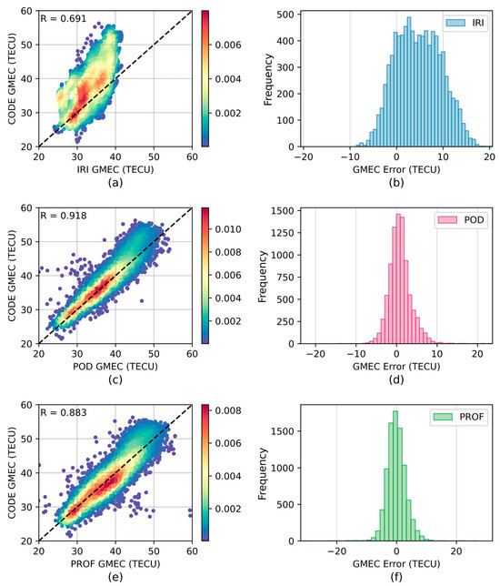
Figure 8.
Scatter density plots (left) and error distribution histograms (right) of GMEC estimates from the IRI-2020 (top), POD (middle), and PROF (bottom) models compared with the CODE GMEC during the 2024 test period.
Overall, as an empirical ionospheric model, IRI-2020 exhibits significant limitations in accurately representing GMEC. Among the two proposed modeling approaches, the POD model demonstrates superior performance, offering the highest prediction accuracy and strongest correlation with the reference values, while the PROF model shows slightly lower performance by comparison.
3.2. GMEC Response to Geomagnetic Storms
The occurrence of geomagnetic storms leads to significant ionospheric disturbances worldwide, with GMEC serving as an important indicator of these disturbances. To assess the responsiveness of the POD GMEC and the PROF GMEC to geomagnetic storms, a case study was conducted on the POD and PROF models during three major geomagnetic disturbance events in 2024.
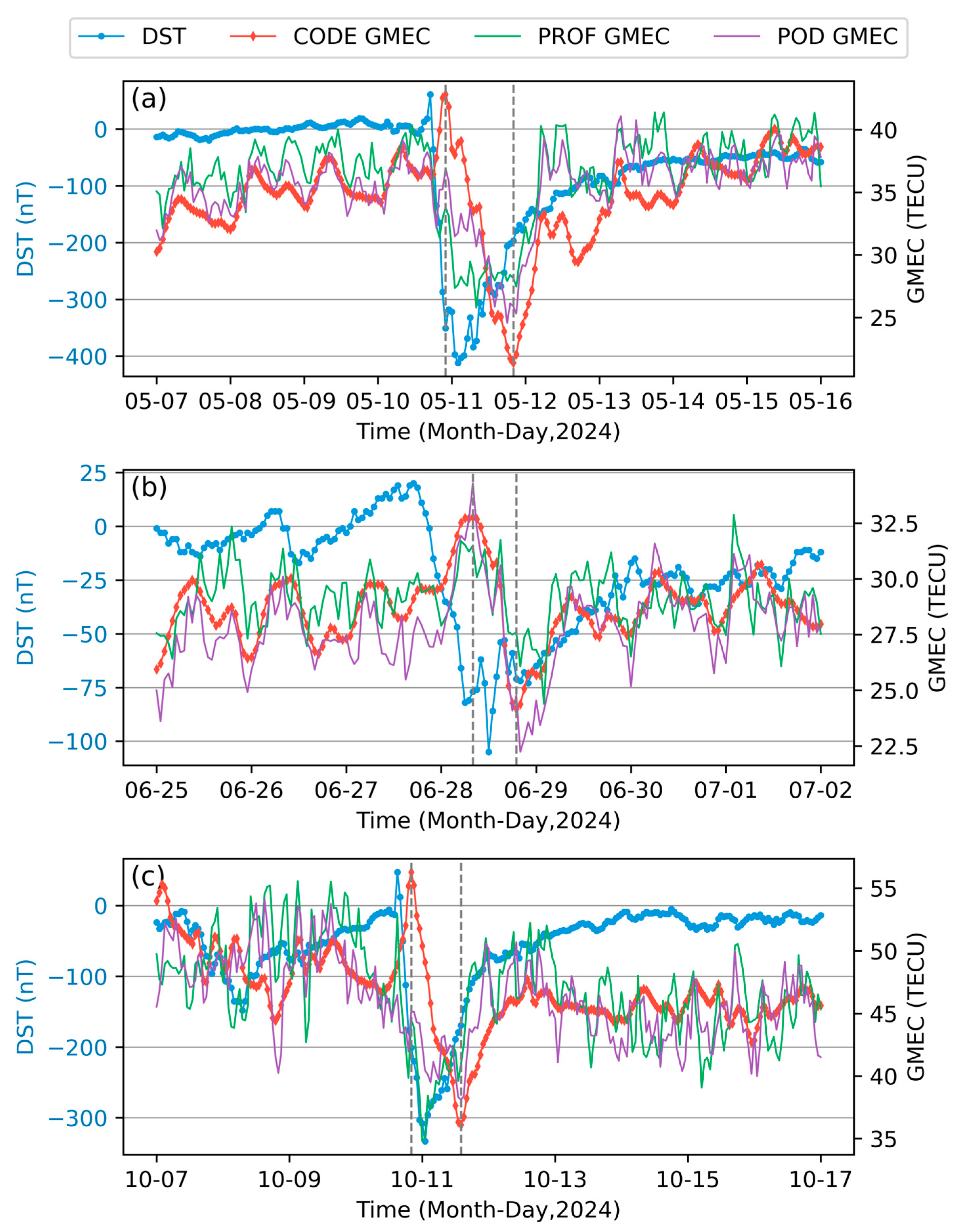
Figure 9 presents the time series of GMEC values alongside the Dst index during these three storm periods. Specifically, Figure 9a–c correspond to the geomagnetic storms that occurred on 10–13 May, 28–29 June, and 10–11 October of 2024, respectively. The minimum Dst values during these events reached –412 nT, –335 nT, and –105 nT, indicating strong storm intensities. The vertical dashed lines in the figure indicate the times of the maximum and minimum values of the CODE GMEC, highlighting the key moments of ionospheric disturbances during each geomagnetic storm. All three events were triggered by coronal mass ejections impacting the Earth’s magnetosphere. Prior to the onset of the storms, the geomagnetic field remained relatively stable with Dst values near zero. Following each storm event, the Dst value gradually recovers back to near zero, indicating the restoration of the geomagnetic field. Notably, significant disturbances in GMEC were observed during each of the three storm periods. A clear correlation was found between storm intensity and GMEC fluctuation magnitude—stronger geomagnetic storms were associated with more pronounced GMEC variations.
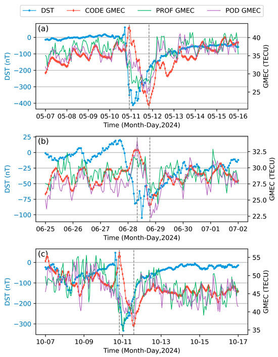
Figure 9.
Time series of CODE GMEC, POD GMEC, PROF GMEC, and Dst index during three geomagnetic storm events in 2024 test set: (a) 7–16 May 2024; (b) 25 June–2 July 2024; (c) 7–17 October 2024.
The CODE GMEC clearly characterizes both the positive and negative phase disturbances of the ionospheric storm induced by geomagnetic storms. Before the storm occurs, the Dst index remains near zero with minor fluctuations, and during this period, the fluctuations in the CODE GMEC are also relatively small. In the initial phase of the storm, the Dst index briefly increases, followed by a rapid decline into the main storm phase, where the Dst index drops sharply into negative values. During this rapid decline in the Dst index, the CODE GMEC also shows a temporary increase, followed by a distinct downward trend. Compared to the Dst index, there is a slight delay in the time at which the CODE GMEC reaches its minimum value. In the recovery phase of the storm, as the Dst value gradually rises back toward zero, the CODE GMEC similarly recovers to a state close to its pre-storm condition. The response of GMEC exhibits a lag effect relative to changes in the magnetic field.
The overall fluctuation trends and intensity changes of the POD GMEC and PROF GMEC before and after geomagnetic storms are consistent with those of the CODE GMEC. During the storm, however, there is a numerical discrepancy between the PROF GMEC and CODE GMEC in terms of the magnitude of the positive phase peak and the negative phase trough. Specifically, after the storm begins, as the Dst index rapidly decreases, both the POD GMEC and PROF GMEC show a positive phase peak. However, the positive phase peak for both the POD GMEC and PROF GMEC is generally lower than that of the CODE GMEC. Once the Dst index reaches its minimum value, the POD GMEC and PROF GMEC also exhibit a minimum value after a brief lag. It is noteworthy that the positive phase peak of the POD GMEC and PROF GMEC after the storm is significantly lower than that of the CODE GMEC, which may be related to the limited coverage of occultation observations. The three geomagnetic storms were caused by coronal mass ejections reaching Earth, with high-energy ions entering the ionosphere through the polar regions. Therefore, after the storm, the CODE GMEC shows a positive phase peak. However, since COSMIC-2’s observational range is limited between latitudes 45° N and 45° S, it is unable to effectively capture ionospheric anomalies in the polar regions, resulting in a smaller response during this phase.
Compared to the CODE GMEC, both the POD GMEC and PROF GMEC exhibit more pronounced fluctuations, with the POD GMEC showing greater instability than the PROF GMEC. This instability may stem from the limited number of radio occultation events available for modeling within each one-hour observation window, making the model more susceptible to the influence of individual measurements. Additionally, the PROF product is derived under the assumption of spherical symmetry, which inherently introduces inversion errors. Despite these factors, the POD GMEC demonstrates better agreement with the CODE GMEC than the PROF GMEC, exhibiting smaller discrepancies in both the timing and magnitude of the minimum values.
3.3. IRI-2020 Model Calibration
To verify the calibration capability of the convolutional neural network with additional GMEC features on the empirical global ionospheric model, the CODE GIM product was used as the reference. Accuracy analysis was performed on the IRI-2020 global TEC map (IRI TEC) and the model corrected using GMEC during both a quiet period (5 January 2024) and a geomagnetic storm period (28 June 2024). Since the POD GMEC has slightly higher accuracy than the PROF GMEC, operates at a lower product level, and does not rely on the spherically symmetric inversion process, only the POD GMEC-Calibrated IRI Global TEC Model (referred to as GCIRI TEC) was analyzed.
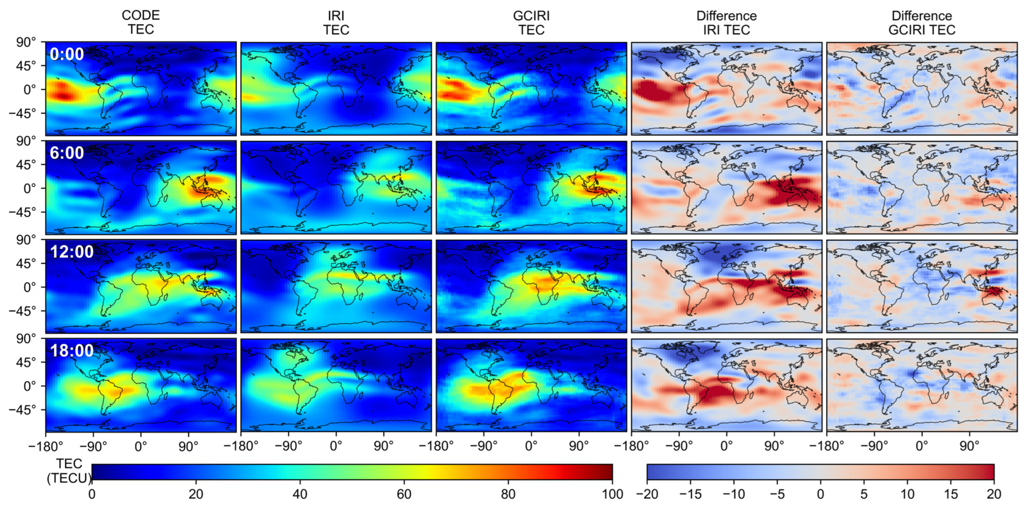
During the ionospheric quiet period, the GCIRI TEC shows a significant improvement in accuracy compared to the IRI TEC model. Figure 10 illustrates the TEC distribution maps for the CODE TEC, IRI TEC, and GCIRI TEC over six-hour intervals on 5 January 2024, during the geomagnetic quiet period, along with the error distribution maps for IRI TEC and GCIRI TEC. From the global TEC distribution, the GCIRI TEC is closer to the CODE TEC than the IRI TEC, both in terms of overall distribution and local details. This is particularly evident in regions of stronger ionospheric activity (higher TEC values), where the GCIRI TEC more accurately reflects the true TEC values. Further analysis of the TEC error distribution shows that the corrected IRI TEC model significantly reduces estimation errors worldwide, with notable improvements in both underestimated and overestimated areas.
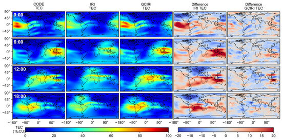
Figure 10.
Difference maps between IRI TEC, GCIRI TEC, and CODE TEC during quiet period (5 January 2024).
Figure 11 presents the error distribution histograms for the GCIRI TEC model and the IRI TEC model over the entire day of 5 January 2024, during the geomagnetic quiet period. The error distribution of the GCIRI TEC model is centered around 0 TECU, with most error values concentrated within ±10 TECU, showing a more focused distribution compared to the IRI TEC model. In contrast, the original IRI TEC model exhibits a more dispersed error distribution with larger errors. The average error (Mean), mean absolute error (MAE), and root mean square error (RMSE) for the IRI TEC model are −0.4 TECU, 6.7 TECU, and 8.8 TECU, respectively. For the GCIRI TEC model, the Mean, MAE, and RMSE are −0.8 TECU, 3.2 TECU, and 4.4 TECU, respectively. The GCIRI TEC model shows improvements of 52.09% and 50.07% in the MAE and RMSE metrics, respectively, indicating a significant increase in accuracy. The experimental results demonstrate that the corrected IRI TEC model exhibits higher accuracy and predictive capability in estimating ionospheric TEC, showing a clear advantage over the original IRI-2020 model.
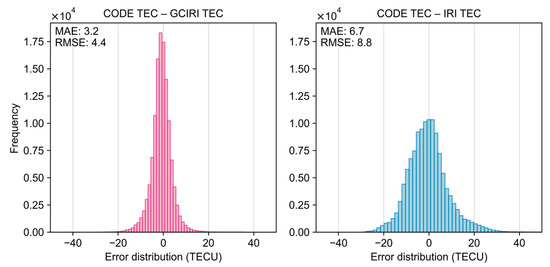
Figure 11.
Error distribution histograms of IRI TEC and GCIRI TEC relative to reference CODE TEC during quiet period (5 January 2024).
Figure 12 presents the variation in RMSE for the GCIRI TEC and IRI TEC relative to the CODE TEC over Universal Time (UT) on 5 January 2024, during a geomagnetically quiet period. Given the stable geomagnetic conditions on that day, the ionosphere remained relatively undisturbed, resulting in minor fluctuations in the TEC. Overall, the RMSE fluctuations of the GCIRI TEC and IRI TEC are both less than 2 TECU, and the temporal variation patterns of RMSE with respect to UT were largely consistent between the two models. Notably, the GCIRI consistently achieved a 4–5 TECU reduction in RMSE compared to IRI, which aligns well with the calibration performance observed in the four representative time periods presented in Figure 10.
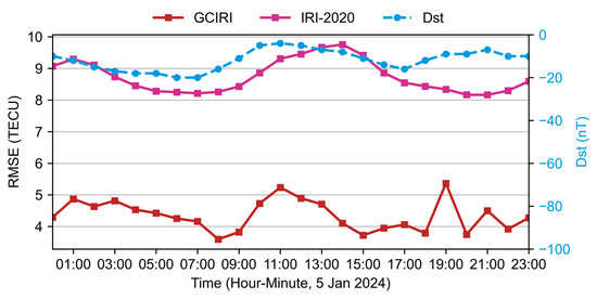
Figure 12.
Variation in RMSE of GCIRI TEC and IRI TEC relative to CODE TEC over UT during quiet period (5 January 2024).
Figure 13 presents RMSE statistics across different latitudes. The IRI TEC exhibits substantial latitudinal variability in RMSE, ranging from 3.8 TECU to 14.1 TECU, with notably inferior performance in low-latitude regions and high-latitude areas of the Southern Hemisphere. In contrast, the GCIRI TEC demonstrates significant accuracy improvements, maintaining RMSE values between 2.6 TECU and 6.7 TECU. Elevated errors for the GCIRI are primarily confined to equatorial latitudes (−20° to 20°), while the most pronounced accuracy enhancements occur at mid-to-high Southern Hemisphere latitudes.

Figure 13.
Variation in RMSE of GCIRI TEC and IRI TEC relative to CODE TEC with latitude during quiet period (5 January 2024).
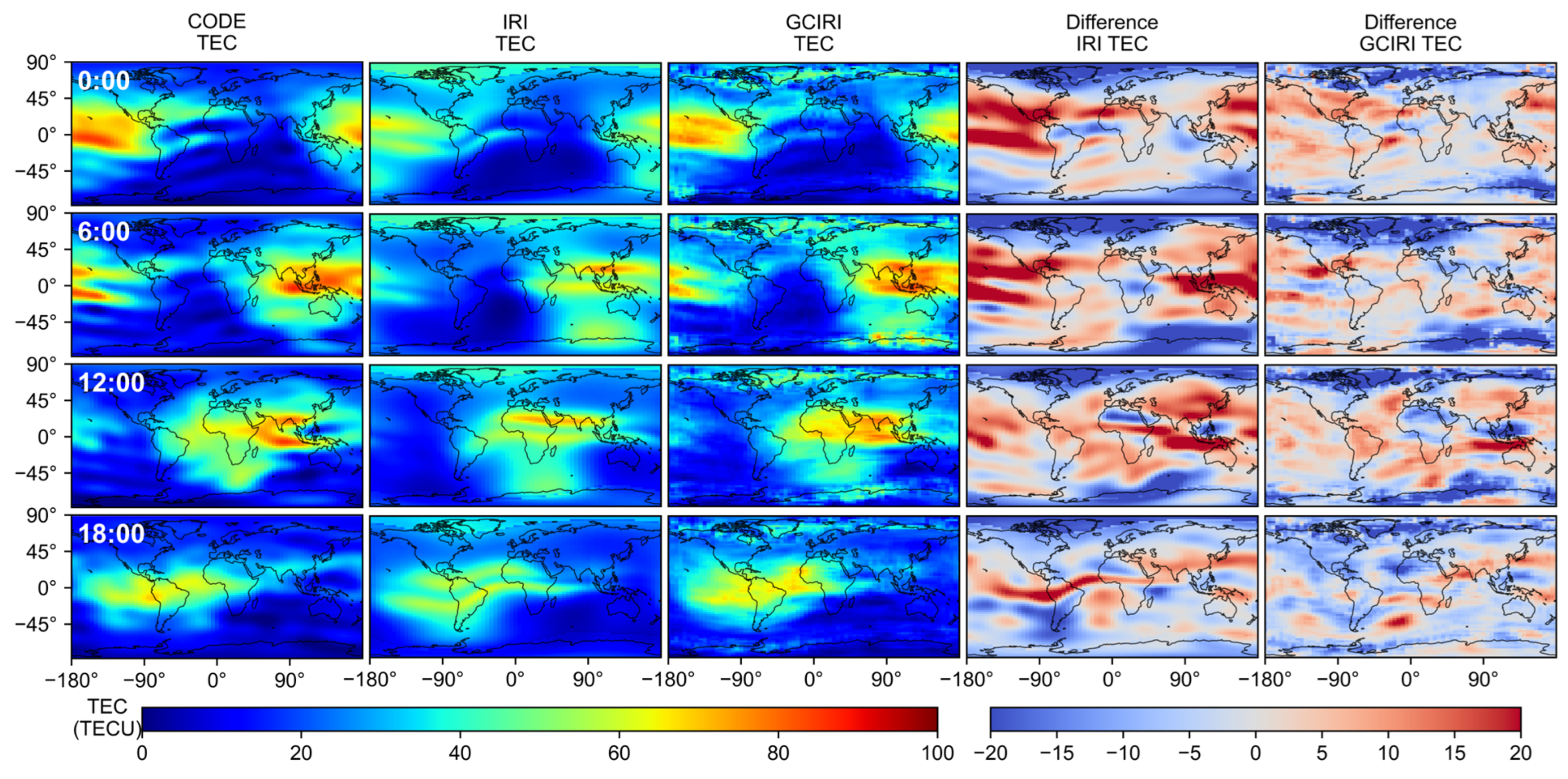
Similarly, during the geomagnetic storm period, the GCIRI TEC also shows a significant improvement in accuracy compared to IRI TEC. Figure 14 presents the difference maps between the IRI TEC, GCIRI TEC, and CODE TEC over six-hour intervals during the geomagnetic storm on 28 June 2024. During the geomagnetic disturbance, the IRI TEC failed to accurately reflect global ionospheric TEC variations, resulting in significant discrepancies with the CODE TEC. Specifically, the error maps revealed substantial regions of both underestimation and overestimation. This indicates that the IRI TEC model exhibits considerable errors in capturing ionospheric changes during geomagnetic storms. In contrast, the GCIRI TEC more accurately mirrors the true global ionospheric TEC variations, with its distribution aligning more closely with the CODE TEC. Additionally, the GCIRI TEC model significantly reduced the areas of underestimation and overestimation in the error maps, demonstrating a higher level of accuracy.
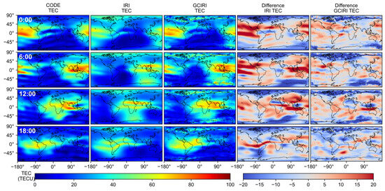
Figure 14.
Difference maps between the IRI TEC, GCIRI TEC, and CODE TEC during the geomagnetic storm period (28 June 2024).
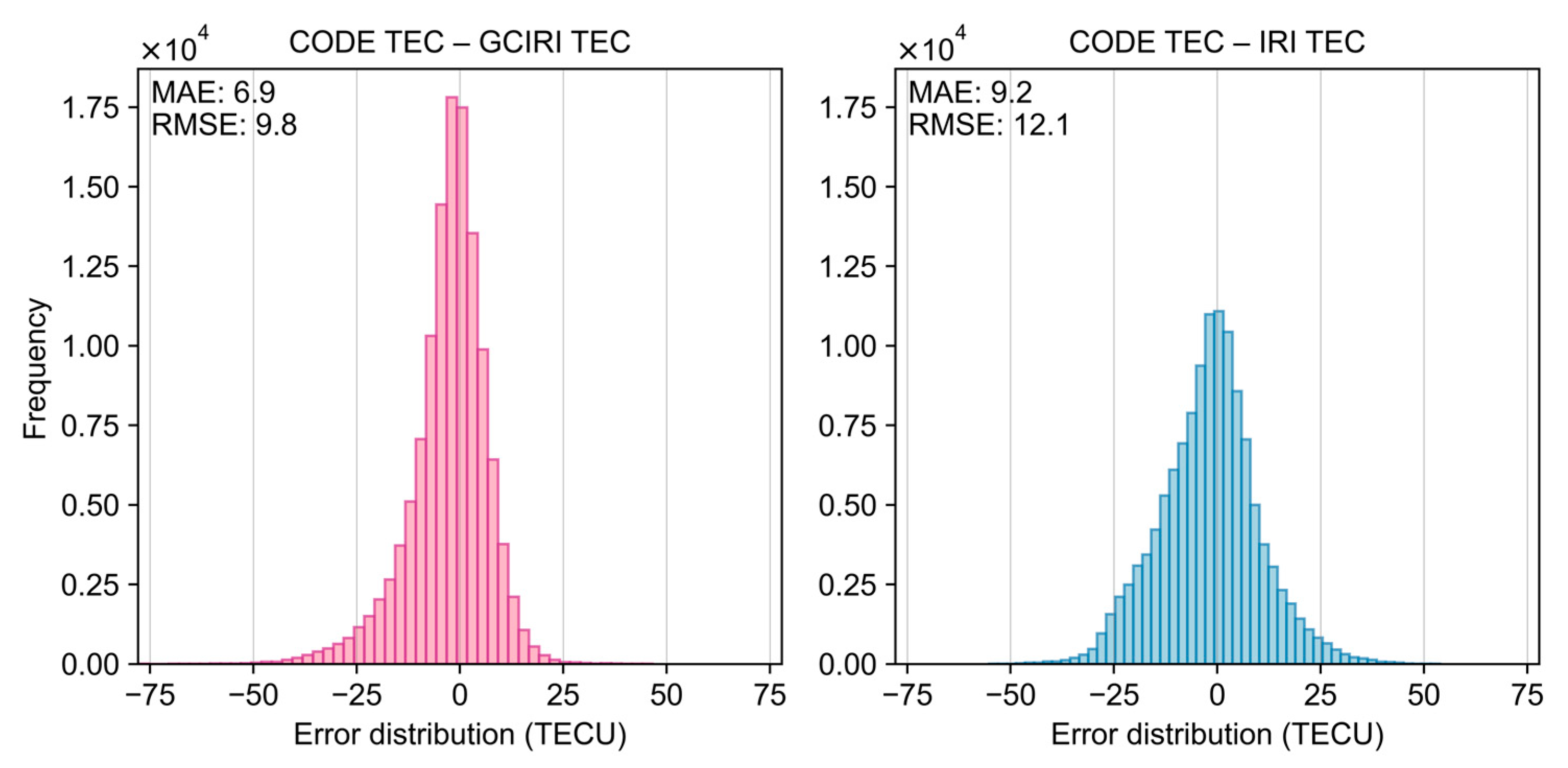
Figure 15 presents the error distribution histograms for the GCIRI TEC and IRI TEC models throughout the entire day during the geomagnetic storm on 28 June 2024. Compared to the original IRI TEC model, the GCIRI TEC model aligns more closely with the CODE TEC. The error distribution of the IRI TEC model has a broader range, spanning from −50 TECU to +50 TECU, while the error distribution of the corrected IRI TEC model is notably narrower, indicating an improvement in accuracy. The IRI TEC model has a Mean, MAE, and RMSE of −1.9 TECU, 9.2 TECU, and 12.1 TECU, respectively. In contrast, the GCIRI TEC model has a Mean, MAE, and RMSE of −2.8 TECU, 6.9 TECU, and 9.8 TECU. The GCIRI TEC model shows improvements of 24.9% in MAE and 19.2% in RMSE, demonstrating enhanced accuracy.
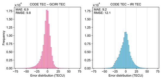
Figure 15.
Error distribution histograms of the IRI TEC and GCIRI TEC relative to the reference CODE TEC during the geomagnetic storm period (28 June 2024).
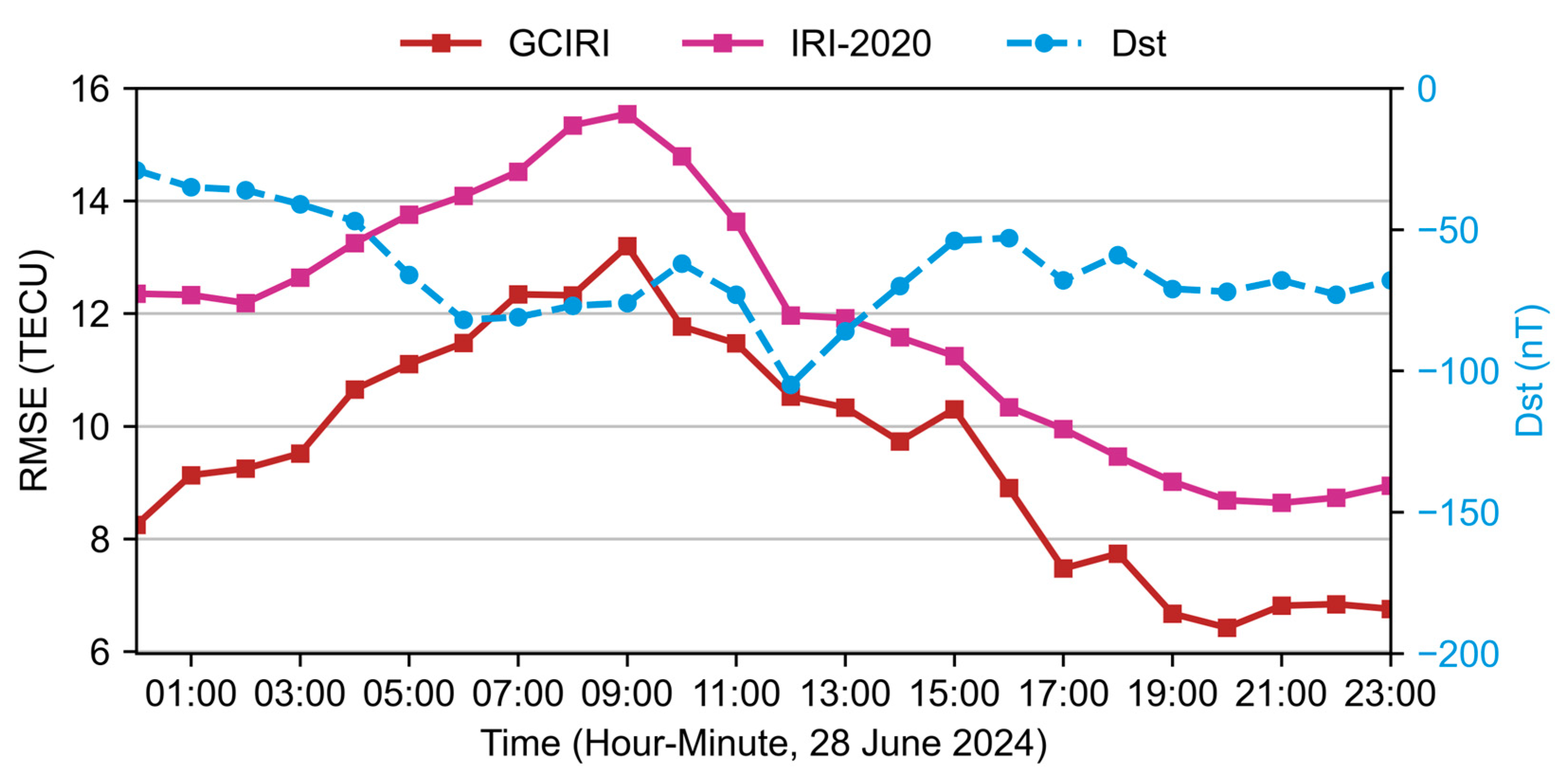
Figure 16 presents the variation in RMSE of the GCIRI TEC and IRI TEC relative to the CODE TEC over UT time during the geomagnetic storm period on 28 June 2024. Under geomagnetically disturbed conditions, ionospheric activity intensifies significantly, resulting in larger fluctuations, with RMSE reaching 12–16 TECU for IRI and 8–13 TECU for GCIRI. Overall, GCIRI exhibits lower RMSE values compared to IRI, with a consistent improvement of approximately 1 to 4 TECU, indicating that GCIRI maintains a certain degree of robustness even under strong geomagnetic disturbances. Notably, starting from 00:00, the RMSE of both models increases gradually, reaching a peak around 09:00, and declining to stabilized low-error levels after 17:00 UT. This diurnal variation closely aligns with the trend of Dst index, reflecting a typical ionospheric response to geomagnetic storm activity.

Figure 16.
Variation in RMSE of GCIRI TEC and IRI TEC relative to CODE TEC over UT during geomagnetic storm period (28 June 2024).
Since the variation in TEC is closely related to both latitude and longitude, and the observational coverage of the COSMIC-2 satellite constellation is geographically constrained, the performance of the GCIRI TEC varies across different regions. In the low- and mid-latitude bands (−45° to 45°), where ionospheric activity is more intense, the IRI model tends to significantly overestimate TEC. In contrast, the GCIRI model demonstrates substantial improvements in this region, providing a more accurate representation of localized ionospheric structures such as equatorial anomalies. At higher latitudes, where ionospheric variability is relatively mild, the IRI model often underestimates TEC. However, due to the limited COSMIC-2 data availability in these regions, the performance gains of GCIRI in high-latitude areas are comparatively modest. In the longitudinal direction, GCIRI exhibits relatively consistent improvements across different longitudes, with no significant variation, primarily because COSMIC-2 observations are uniformly distributed in longitude.
It is worth noting that the GCIRI TEC model exhibits an uneven structure in the polar regions. This may be due to the non-smooth edges of the IRI TEC in the polar regions during geomagnetic storms, a feature that the convolutional neural network captures and amplifies in the reconstructed image. The new model shows limitations in overcoming this non-smooth edge effect, which should be taken into consideration during its application. In addition, Figure 10 and Figure 14 reveal noticeable small-scale variations in the GCIRI TEC, along with slight numerical discontinuities. These features highlight a current limitation of the CNN model. Nevertheless, the accuracy of the GCIRI TEC model during geomagnetic storms is significantly superior to that of the original IRI TEC model. Overall, the GCIRI TEC model demonstrates relatively good performance both during geomagnetic quiet periods and storm periods.
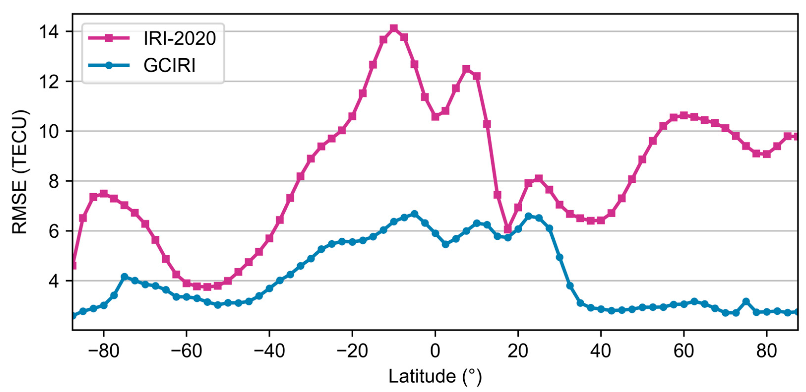
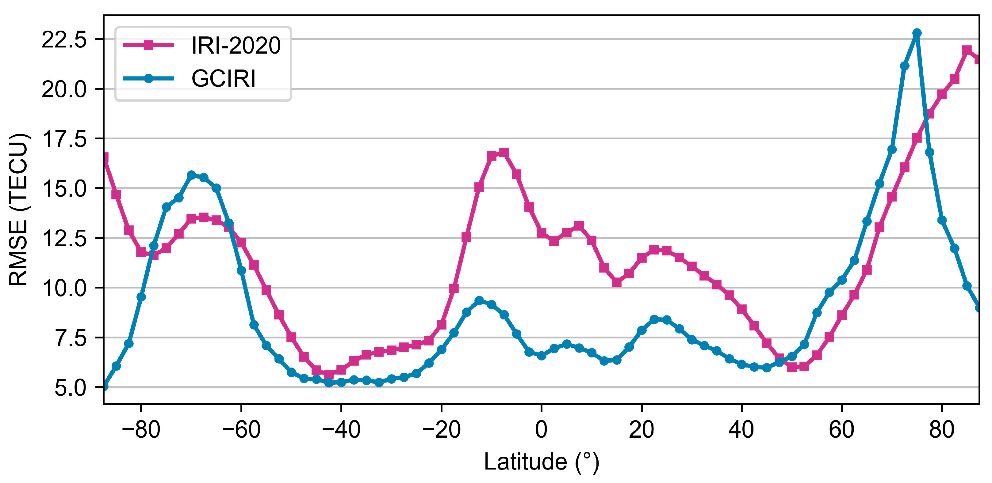
Figure 17 displays latitude-dependent RMSE distributions for the selected day. The IRI TEC exhibits substantial RMSE variability (5–22 TECU) across latitudes, with degraded accuracy particularly evident in low- and high-latitude regions. Similarly, the GCIRI TEC demonstrates significant accuracy improvements at mid–low latitudes (−20° to 40°). However, GCIRI underperforms IRI in polar regions beyond ±70° latitude—a limitation likely attributable to COSMIC-2’s observational gap in these areas.
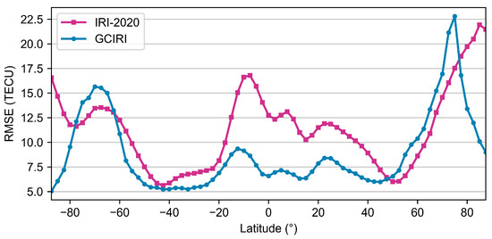
Figure 17.
Variation in RMSE of GCIRI TEC and IRI TEC relative to CODE TEC with latitude during geomagnetic storm period (28 June 2024).
Furthermore, the accuracy of the IRI TEC and GCIRI TEC throughout the year 2024 was compared. Figure 18 presents a time series histogram of the monthly average RMS differences between the IRI-2020 model and CODE GIM, before and after calibration. As shown in the figure, the RMS values after calibration are consistently lower than those before calibration. This improvement is particularly notable during the peak months of September, October, and November. Before calibration, the monthly RMS values ranged from a minimum of 11.5 TECU to a maximum of 22.9 TECU, with an annual mean of 15.8 TECU. After calibration, the RMS values were significantly reduced, with a minimum of 5.2 TECU, a maximum of 17.1 TECU, and an annual mean of 11.1 TECU. Overall, the RMS was improved by 29.9% over the course of 2024. These results demonstrate that the calibrated model significantly enhances the accuracy of the IRI-2020 model, improves its performance under complex ionospheric conditions, and substantially reduces discrepancies with the CODE GIM. This highlights the effectiveness of the calibration in refining empirical ionospheric modeling.
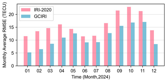
Figure 18.
Monthly average RMSE histograms of the IRI TEC and GCIRI TEC relative to the reference CODE TEC in the 2024 test set.
4. Discussion
Based on space-based GNSS radio occultation observations and machine learning methods, we have developed a GMEC model independent of traditional ground-based GNSS data and used GMEC and machine learning techniques to calibrate empirical ionospheric TEC models.
The L1b-level STEC observation data from the COSMIC-2 satellites provide a new data dimension for GMEC modeling. Their global coverage effectively fills the observational gaps left by ground-based GNSS, especially in oceanic and polar regions (Figure 2). Notably, the POD solution, based on raw STEC observations, demonstrates superior accuracy (correlation coefficient of 0.918) compared to the PROF solution, which uses Abel inversion-derived data (correlation coefficient of 0.883). This discrepancy may be due to the limitations of the spherical symmetry assumption. In the electron density inversion process, the horizontal gradient of the ionosphere is simplified, leading to the introduction of errors in the PROF solution [24]. In contrast, the POD solution avoids such systematic errors by directly utilizing line-of-sight path TEC observations.
In terms of magnetic storm response mechanisms, both the POD GMEC and PROF GMEC exhibit phase characteristics synchronized with the CODE GIM. However, they show insufficient amplitude in the positive phase response during ionospheric storms. This discrepancy may be attributed to the lack of observational coverage in the polar regions by the COSMIC-2 satellites (Figure 2). The ionospheric storm response in the polar regions has been confirmed as a key process driving ionospheric changes during magnetic storms [25,26]. These findings suggest that future model optimizations should focus on addressing the issue of missing data in the polar regions.
GMEC reflects the overall state of the global ionosphere and can be used to calibrate global empirical TEC models. Unlike the approaches of Zhang Wen et al. [27] and Liu Lei et al. [28], who use updated IG index-driven IRI models, we employ convolutional neural networks (CNNs) with a 5 × 5 convolution kernel to extract features from the IRI grid (see Figure 6). This approach establishes a nonlinear mapping relationship between ionospheric disturbances and global features (GMEC) in the spatial dimension. Similarly, Gao Xin et al. [14] proposed an IRI-2020 ionospheric TEC reconstruction method, which constructs four input grid channels based on factors like F10.7, SSN, Dst index, and Kp index, along with the TEC grid channel of IRI-2020 for model training. The model’s accuracy was improved by 40.8% during quiet periods and 43% during magnetic storm periods. In comparison, the architecture of our model is simpler, using only the GMEC single factor as an additional feature to construct the CNN. In terms of calibration performance, our method demonstrated a higher accuracy improvement during quiet periods, reaching 50.1%, while the improvement during magnetic storm periods was slightly lower at approximately 28.5%. This difference may be due to missing data in the polar regions during magnetic storms. Future improvements could involve increasing the availability of polar region observations to enhance GMEC estimation accuracy. Furthermore, the CNN model developed in this study still exhibits certain limitations. Although the GCIRI TEC demonstrates a significant improvement in accuracy compared to the IRI TEC, the results show noticeable small-scale TEC variations and slight numerical discontinuities. These artifacts indicate that the current model still has room for improvement in terms of spatial continuity and smoothness.
5. Conclusions
In this study, an equivalent global mean TEC model was developed using the backpropagation neural network (BPNN) method, with COSMIC-2 occultation data and the solar activity index F10.7 as inputs for training. The ionPrf and podTc2 products from COSMIC-2, as well as CODE GIM TEC grid maps with a 1 h time resolution, were collected from 2019 to 2024 to calculate the corresponding global mean TEC (GMEC). F10.7 was used as an additional feature for model training. The GMEC was then evaluated using a test set based on 2024 data. Compared to the IRI GMEC, the equivalent global mean TEC models (POD GMEC and PROF GMEC), trained using the BPNN method, showed good agreement with the reference true value, CODE GMEC, in terms of trend variations. This indicates that, despite the limited spatial coverage of COSMIC-2 observations, these data still possess a strong capability to represent global ionospheric variability. Furthermore, the estimated POD GMEC and PROF GMEC demonstrated similar responses to magnetic storm events as CODE GMEC. However, both GMEC models showed a weak response to the positive phase ionospheric disturbances following the magnetic storms, which may be attributed to the lack of observational data from the polar regions.
Furthermore, we propose a convolutional neural network (CNN) approach that uses global mean TEC (GMEC) as an additional feature to calibrate the IRI-2020 global TEC model. The accuracy of the calibrated model was then evaluated to assess GMEC’s ability to calibrate the empirical global ionospheric TEC model. Experimental results demonstrate that, compared to the original IRI-2020 empirical model, the IRI TEC model calibrated with the POD GMEC significantly reduces the difference between the IRI TEC and CODE TEC, while better capturing ionospheric variations during magnetic storm periods. The calibrated IRI TEC model showed accuracy improvements of 50.1% during geomagnetic quiet periods and 28.5% during magnetic storm periods compared to the original IRI TEC model. The lower correction accuracy during magnetic storms may be attributed to the weak GMEC response due to insufficient polar region observations.
Future research could consider acquiring additional ionospheric observation data from the polar regions to further improve the estimation accuracy of the global mean TEC and enhance the calibration effectiveness of the IRI-2020 model.
6. Patents
The technology related to the findings of this study has been granted a patent by the China National Intellectual Property Administration (CNIPA), with the patent number [ZL 2025 1 0170773.2].
Author Contributions
Conceptualization, Y.L., W.W. and L.Z.; methodology, L.Z.; software, Y.L. and L.Z.; validation, Y.L. and L.Z.; formal analysis, Y.L. and L.Z.; investigation, Y.L.; resources, Y.Y. and L.Z.; data curation, Y.L.; writing—original draft preparation, Y.L.; writing—review and editing, L.Z.; visualization, Y.L.; supervision, L.Z.; project administration, L.Z. and Y.Y.; funding acquisition, Y.Y. All authors have read and agreed to the published version of the manuscript.
Funding
This research was funded by the National Natural Science Foundation of China, Grant No. 42304022, 42388102, 42330105; the Wuhan Natural Science Foundation Exploration Program: Chenguang Program, Grant No 2024040801020237; and Nanning Major Science and Technology Project, Grant No 20241027.
Data Availability Statement
The COSMIC-2 products were obtained online (https://data.cosmic.ucar.edu/gnss-ro/cosmic2/, accessed on 12 October 2024). The solar index F10.7 and Dst index products were obtained from the website (https://omniweb.gsfc.nasa.gov/form/dx1.html, accessed on 25 October 2024).
Acknowledgments
The authors would like to thank UCAR for providing the COSMIC-2 ionPrf and podTc2 products.
Conflicts of Interest
The authors declare no conflicts of interest.
References
- Jakowski, N. Ionosphere Monitoring. In Springer Handbook of Global Navigation Satellite Systems; Teunissen, P.J.G., Montenbruck, O., Eds.; Springer International Publishing: Cham, Germany, 2017; pp. 1139–1162. [Google Scholar]
- Bust, G.S.; Mitchell, C.N. History, Current State, and Future Directions of Ionospheric Imaging. Rev. Geophys. 2008, 46, 000212. [Google Scholar] [CrossRef]
- Hocke, K. Oscillations of Global Mean TEC. J. Geophys. Res. Space Phys. 2008, 113, 012798. [Google Scholar] [CrossRef]
- Hernández-Pajares, M.; Juan, J.M.; Sanz, J.; Orus, R.; Garcia-Rigo, A.; Feltens, J.; Komjathy, A.; Schaer, S.C.; Krankowski, A. The IGS VTEC Maps: A Reliable Source of Ionospheric Information since 1998. J. Geod. 2009, 83, 263–275. [Google Scholar] [CrossRef]
- Huang, D.; Huang, C.; Li, J.; Yan, H.; Yu, N. GPS Radio Occultation Technology for Monitoring Earth’s Atmosphere. Adv. Earth Sci. 1997, 12, 217–223. [Google Scholar] [CrossRef]
- Xue, Z.; Bao, Y.; Tang, G.; Cheng, W.; Zhu, M.; Yuan, S. Quality Analysis of COSMIC-2 Occultation Inversion Data. Remote Sens. Technol. Appl. 2022, 38, 453–466. [Google Scholar] [CrossRef]
- Liu, J.; Zhao, Y.; Zhang, X. Current Status and Prospect of GNSS Radio Occultation Ionosphere Inversion Technology. J. Wuhan Univ. Technol. 2010, 35, 631–635. [Google Scholar]
- McGranaghan, R.M.; Mannucci, A.J.; Verkhoglyadova, O.; Malik, N. Finding Multiscale Connectivity in Our Geospace Observational System: Network Analysis of Total Electron Content. J. Geophys. Res. Space Phys. 2017, 122, 7683–7697. [Google Scholar] [CrossRef]
- Liu, L.; Zou, S.; Yao, Y.; Wang, Z. Forecasting Global Ionospheric TEC Using Deep Learning Approach. Space Weather 2020, 18, e2020SW002501. [Google Scholar] [CrossRef]
- Liu, L.; Morton, Y.J.; Liu, Y. ML Prediction of Global Ionospheric TEC Maps. Space Weather 2022, 20, e2022SW003135. [Google Scholar] [CrossRef]
- Olwendo, O.J.; Baki, P.; Cilliers, P.J.; Mito, C.; Doherty, P. Comparison of GPS TEC Variations with IRI-2007 TEC Prediction at Equatorial Latitudes During a Low Solar Activity (2009–2011) Phase over the Kenyan Region. Adv. Space Res. 2013, 52, 1770–1779. [Google Scholar] [CrossRef]
- Rao, S.S.; Chakraborty, M.; Kumar, S.; Singh, A.K. Low-Latitude Ionospheric Response from GPS, IRI and TIE-GCM TEC to Solar Cycle 24. Astrophys. Space Sci. 2019, 364, 216. [Google Scholar] [CrossRef]
- Shi, C.; Zhang, T.; Wang, C.; Wang, Z.; Fan, L. Comparison of IRI-2016 Model with IGS VTEC Maps During Low and High Solar Activity Period. Results Phys. 2019, 12, 555–561. [Google Scholar] [CrossRef]
- Gao, X.; Yao, Y.; Wang, Y. Reconstruction of Global Ionospheric TEC Maps from IRI-2020 Model Based on Deep Learning Method. J. Geod. 2024, 98, 10. [Google Scholar] [CrossRef]
- Weiss, J.-P.; Schreiner, W.S.; Braun, J.J.; Xia-Serafino, W.; Huang, C.-Y. COSMIC-2 Mission Summary at Three Years in Orbit. Atmosphere 2022, 13, 1409. [Google Scholar] [CrossRef]
- Lu, H.; Ye, S.; Zhang, Q.; Xia, P.; E, S. Analysis of the Spatiotemporal Variations of the Ionosphere in China over the Past 15 Years Using COSMIC-1/2 IonPrf Products. J. Wuhan Univ. Technol. 2024, 49, 765–774. [Google Scholar] [CrossRef]
- Tapping, K.F. The 10.7 Cm Solar Radio Flux (F10.7). Space Weather 2013, 11, 394–406. [Google Scholar] [CrossRef]
- Schaer, S.; Helvétique des Sciences Naturelles; Commission Géodésique. Mapping and Predicting the Earth’s Ionosphere Using the Global Positioning System; Institut für Geodäsie und Photogrammetrie an der Eidg, Technische Hochschule Zürich: Zürich, Switzerland, 1999; Volume 59. [Google Scholar]
- Ren, X.; Yang, P.; Liu, H.; Chen, J.; Liu, W. Deep Learning for Global Ionospheric TEC Forecasting: Different Approaches and Validation. Space Weather 2022, 20, e2021SW003011. [Google Scholar] [CrossRef]
- Afraimovich, E.L.; Astafyeva, E.I.; Oinats, A.V.; Yasukevich, Y.V.; Zhivetiev, I.V. Global Electron Content: A New Conception to Track Solar Activity. Ann. Geophys. 2008, 26, 335–344. [Google Scholar] [CrossRef]
- Rawer, K.; Bilitza, D.; Ramakrishnan, S. Goals and Status of the International Reference Ionosphere. Rev. Geophys. 1978, 16, 177–181. [Google Scholar] [CrossRef]
- Bilitza, D.; Altadill, D.; Truhlik, V.; Shubin, V.; Galkin, I.; Reinisch, B.; Huang, X. International Reference Ionosphere 2016: From Ionospheric Climate to Real-Time Weather Predictions. Space Weather 2017, 15, 418–429. [Google Scholar] [CrossRef]
- Bilitza, D.; Pezzopane, M.; Truhlik, V.; Altadill, D.; Reinisch, B.W.; Pignalberi, A. The International Reference Ionosphere Model: A Review and Description of an Ionospheric Benchmark. Rev. Geophys. 2022, 60, e2022RG000792. [Google Scholar] [CrossRef]
- Aragon-Angel, A.; Hernandez-Pajares, M.; Zornoza, J.M.J.; Subirana, J.S. Improving the Abel Transform Inversion Using Bending Angles from FORMOSAT-3/COSMIC. GPS Solut. 2010, 14, 23–33. [Google Scholar] [CrossRef]
- Mendillo, M. Storms in the Ionosphere: Patterns and Processes for Total Electron Content. Rev. Geophys. 2006, 44, 000193. [Google Scholar] [CrossRef]
- Gulyaeva, T.L.; Veselovsky, I.S. Two-Phase Storm Profile of Global Electron Content in the Ionosphere and Plasmasphere of the Earth. J. Geophys. Res. Space Phys. 2012, 117, 018017. [Google Scholar] [CrossRef]
- Zhang, W.; Huo, X.; Yuan, Y.; Li, Z.; Wang, N. Algorithm Research Using GNSS-TEC Data to Calibrate TEC Calculated by the IRI-2016 Model over China. Remote Sens. 2021, 13, 4002. [Google Scholar] [CrossRef]
- Liu, L.; Yao, Y.; Zou, S.; Kong, J.; Shan, L.; Zhai, C.; Zhao, C.; Wang, Y. Ingestion of GIM-Derived TEC Data for Updating IRI-2016 Driven by Effective IG Indices over the European Region. J. Geod. 2019, 93, 1911–1930. [Google Scholar] [CrossRef]


Disclaimer/Publisher’s Note: The statements, opinions and data contained in all publications are solely those of the individual author(s) and contributor(s) and not of MDPI and/or the editor(s). MDPI and/or the editor(s) disclaim responsibility for any injury to people or property resulting from any ideas, methods, instructions or products referred to in the content. |
© 2025 by the authors. Licensee MDPI, Basel, Switzerland. This article is an open access article distributed under the terms and conditions of the Creative Commons Attribution (CC BY) license (https://creativecommons.org/licenses/by/4.0/).