Article

Disagreements in Equivalent-Factor-Based Valuation of County-Level Ecosystem Services in China: Insights from Comparison Among Ten LULC Datasets

1
Department of Land Resource Management, School of Public Administration, China University of Geosciences, Wuhan 430074, China
2
Wuhan Planning & Design Institute (Wuhan Transportation Development Strategy Institute), Wuhan 430014, China
3
Key Laboratory of the Ministry of Natural Resources for Research on the Rule of Law, 388 Lumo Road, Hongshan District, Wuhan 430074, China
*
Author to whom correspondence should be addressed.
Remote Sens. 2025, 17(13), 2320; https://doi.org/10.3390/rs17132320
Submission received: 16 May 2025 / Revised: 1 July 2025 / Accepted: 1 July 2025 / Published: 6 July 2025

Abstract

Valuation of ecosystem services (ESs) is crucial for understanding the benefits provided by ecosystems and informing sustainable management and policy decisions related to ecosystem protection. This study explores the disagreements in ecosystem service value (ESV) at the county level across China in 2020 by comparing ten land cover datasets of varying resolutions from 500 to 10 m, using the equivalent factor method. Significant disagreements in ESV estimates are identified, revealing spatial heterogeneity and large inconsistencies among estimates from different datasets, even with high spatial resolution (10 m). Across all counties, the typical discrepancy in ESV estimates between any two datasets reaches 3503 CNY/ha, and the ESV estimates for each county show an average coefficient of variation (CV) of 0.186 across the ten datasets, indicating considerable inconsistency attributable to dataset selection. The results highlight that ESV evaluations based on the CLCD, Globeland30, and GLC-FCS30 datasets demonstrate higher consistency and reliability, making them suitable for regional ecosystem service valuation. Both the landscape configurations and the area disparities of different land types have significant impacts on ESV disagreement. This study provides valuable insights into the applicability of different datasets for ESV evaluation, thereby enhancing the reliability of ESV assessments and supporting informed decision making in ecosystem management.

1. Introduction

Evaluating ecosystem services (ESs) is fundamental to understanding the ecological, economic, and social benefits natural ecosystems provide [1,2]. These evaluations inform natural resources management, conservation strategies, and adaptation finance flows by quantifying these benefits in monetary terms. However, due to differences in data sources, there have traditionally been considerable disagreements in estimates of ESV [3,4]. For example, from previous studies, ESV estimates of Wuhan, China, range from CNY 5.28 billion to CNY 114.847 billion [5,6], with a percentage difference of up to 182.42%, affecting the reliability and applicability of the results. Quantifying these disagreements is crucial, as it enhances transparency in ESV evaluations and helps decision makers and stakeholders better understand the potential risks and limitations associated with valuation results [7,8]. Moreover, by addressing disagreements, decision makers can better allocate finance flows, prioritize conservation efforts, and set realistic expectations for ecosystem management outcomes [9].
Among various valuation approaches, the equivalent factor method, initially proposed by Costanza et al. [10], has been widely used worldwide due to its standardized framework, operational simplicity, and good explainability [11]. Internationally, this method has been applied across diverse ecological and socio-economic contexts, including global- and continental-scale ecosystem assessments [10,12], global wetland evaluations [13], and regional studies in European [14], African [15,16], and American watersheds [17]. These applications highlight their versatility and widespread acceptance as a practical tool for ecosystem service valuation. Building upon these international applications, the method was further introduced and revised in China by Xie and his colleagues [18,19] through a series of surveys involving 500 Chinese ecologists to better align the framework with China’s diverse ecological conditions. Given its ease of application at large scales, the equivalent factor method has been extensively adopted for regional and national ESV assessments in China, providing important references for ecological conservation planning and policy initiatives. Regional ESV estimated based on the equivalent factor method has important references for guiding payment for ecosystem services programs in China [20,21]. Previous research indicates that more than half of ESV-related studies have relied on this approach [21,22]. Therefore, ESV estimates derived from the equivalent factor method have played—and will continue to play—a significant role in ecosystem management.
A critical prerequisite for employing the equivalent factor method in ESV evaluation is the availability of high-quality land cover data [23]. In recent decades, the proliferation of global satellite imagery and advancements in remote sensing techniques have led to the creation of numerous freely accessible land cover datasets at both global and national scales [24]. These data products are the essential basis for ESV assessments at regional, national, and global levels. Researchers and decision makers widely utilize these freely available land cover datasets, particularly for large-scale ESV evaluations. For example, the ESRI data developed by the European Space Agency [25], the CGLS_LC100 product from the Copernicus Global Land Service [26], the GlobCover data from the European Space Agency [27], and the ESA_CCI land cover dataset [28] have provided crucial support for ESV assessments at various scales.
Chinese researchers have also contributed to the development of several global- and national-scale land cover datasets, such as the FROM-GLC dataset developed by Tsinghua University [29], the CLCD dataset developed by Wuhan University [30], the Globeland30 dataset developed by the National Geomatics Center of China [31], the GLC_FCS30 dataset developed by the Chinese Academy of Sciences [32], and the CNLUCC dataset [33]. Among these datasets, CLCD, CNLUCC, ESRI, ESA_CCI, and Globeland30 have been used for regional- and national-scale ESV assessments in China. Comparatively, ESV evaluations based on datasets such as AI Earth [34], CGLS_LC100, GLC_FCS30, MDC12Q1 [35], and World Cover [36] are seldom reported in national-scale ES valuation in China. These datasets are expected to become more widely used in future ESV estimates, as researchers and decision makers often assume that high-resolution land cover datasets inherently yield more reliable and accurate results. However, this assumption does not always hold true in practice, as high-resolution datasets may introduce their complexities and potential sources of disagreement [37].
Due to variations in satellite sensors, land cover classification systems, and interpretation methodologies used to generate land cover datasets, significant inconsistencies often arise in the mapped land cover patterns across different datasets [38,39]. Most existing comparative studies on land cover datasets have primarily focused on evaluating classification accuracy, consistency, and thematic agreement across products [40,41,42,43], for example, through pixel-based comparison, confusion matrix analysis, or spatial overlap metrics. However, less attention has been paid to how these differences in land cover representations translate into inconsistencies in downstream ecological applications, particularly in ecosystem service valuation (ESV). In reality, even slight differences in land cover classification can significantly influence ecosystem types’ estimated extent and distribution, leading to diverging ESV results. As a result, substantial discrepancies exist in regional ESV estimates derived from different land cover datasets using the equivalent factor method. For example, researchers estimated Beijing’s ESV in 2000 to be CNY 28.211 billion [44] and CNY 21.061 billion [45], respectively, revealing a considerable difference of 29%. Similarly, different studies [46,47] estimated the ESV of the Sanjiang Plain in the same year to be CNY 166.029 billion and CNY 134.417 billion, respectively, reflecting a 21% difference. These examples highlight the substantial disagreements and pervasive inconsistencies in ESV evaluations that arise from differences in data sources.
Previous studies have explored the disagreement in ESV evaluations arising from using various land cover datasets [48]. For instance, Schulp, et al. [49] conducted a quantitative comparative analysis of the disagreements associated with different data sources for five Europe ecosystem services. Their results indicated significant disagreements in ESV estimates for erosion protection and flood regulation services. Similarly, Song [50] utilized nine global land cover datasets to quantify the annual average value and its fluctuation range of global ecosystem services, which varied between USD 35.0 and 56.5 trillion annually. Also, ESVs estimated following the equivalent factor method can differ from those estimated by the other methods [21,51]. These studies acknowledge the inconsistency in ESV assessment results when different land cover datasets are employed, highlighting the importance of carefully considering the impact of dataset selection on ESV outcomes.
Although existing research has made progress in identifying the disagreements of ESV assessments derived from different land cover products, several limitations remain. For instance, few studies have conducted quantitative analyses of the spatial heterogeneity of disagreement in county-level ESV assessments that involve the latest high-resolution land cover datasets. Additionally, explicit indications of the applicability of different land cover products for ESV assessment are still lacking at the national and county levels. Furthermore, previous research investigating these inconsistencies primarily relied on earlier-generation datasets, typically with coarser spatial resolutions (around 1 km) [52]. Several new land use and land cover products offer a very high resolution of 10 m. However, recent comparative analyses of these high-resolution datasets, primarily within the field of remote sensing, mainly focus on specific regions or emphasize the comparison of product accuracy rather than evaluating their inconsistency in ESV estimations. In order to conduct further research, this study incorporates widely used land cover datasets and systematically quantifies their impact on ESV estimates. It further identifies spatial heterogeneity in disagreements and provides region-specific recommendations to support more informed dataset selection in ecosystem service assessments.
Using the equivalent factor method, we employ ten land cover data products with varying resolutions, interpretation accuracies, and classification systems to evaluate and compare county-level ESVs in China. These datasets encompass nearly all applicable land cover datasets with medium to high spatial resolution, ranging from 500 m to 10 m. The primary objectives of this study are to (1) quantify the magnitude and spatial heterogeneity of ESV disagreements arising from different land cover datasets at the county level, (2) evaluate the applicability and consistency of each dataset for ESV assessments, and (3) explore the potential drivers of ESV inconsistency, including landscape configuration and ecosystem type area disagreement. Through these objectives, this study seeks to enhance the reliability of ESV evaluated using the equivalent factor method. It provides a valuable reference for choosing fit-for-county datasets for ecosystem service evaluation and management. The findings can inform the stakeholders to pay attention to the disagreement of ESV in the management of ESs.

2. Materials

2.1. Study Area and Evaluation Units of ESV

China hosts various ecosystems due to its vast territory, diverse topography, and climate. Grasslands, forests, croplands, and deserts are the dominant types, covering 82.8% of the national land area [53]. Forests and croplands prevail in the eastern monsoon region, grasslands and deserts dominate the arid northwest, and the Qinghai–Tibet Plateau features unique alpine meadows, deserts, and permafrost. In China, the county or district is the basic administration unit for policymaking regarding ecosystem management. Therefore, this study selected 2898 county- or district-level administrative units in China as the evaluation units based on the geographic information dataset publicly released by the National Geomatics Center of China in 2021. The ESV of these units for 2020 was assessed using ten different land cover data products. Subsequently, the disagreement in the ESV estimates across these units was quantitatively analyzed.

2.2. Data Sources and Preprocessing

2.2.1. Land Cover Data

This study employed ten widely used land cover datasets for ESV assessment. These ten datasets were selected based on two criteria: (1) full spatial coverage of China and (2) data availability for 2020 or close to it. The datasets include both global-scale products, such as AI Earth [34], CGLS_LC100 [26], ESA_CCI [28], ESRI [25], GLC_FCS30 [32], Globeland30 [31], MDC12Q1 [35], and World Cover [36], as well as China-specific products, such as CLCD [30] and CNLUCC [33]. These raster datasets have spatial resolutions ranging from 10 to 500 m and utilize different land cover classification systems and interpretation methods. Table S1 in the Supplemental Materials provides detailed information on these land cover datasets. Since the CGLS-LC100 dataset does not have data available for 2020, the most recent data from 2019 was used as a substitute. Given that the actual land cover change within one year is negligible compared to the differences among datasets, this substitution is considered acceptable in large-scale analyses [54].

2.2.2. Data Processing

To minimize the influence of spatial projection distortion in the area summation of different land types within each county, the coordinate systems of all ten datasets were uniformly converted to the Krasovsky_1940_Albers equal-area projection (central meridian: 104°E; first standard parallel: 25°N; second standard parallel: 47°N). Subsequently, invalid pixel values in the land cover datasets were removed. For instance, ocean-related pixels in the CNLUCC dataset were excluded since this study focuses solely on terrestrial ecosystems. Similarly, default pixel values or those representing cloud cover in the GLC-FCS30 and ESRI datasets were also eliminated to prevent them from affecting the subsequent assessments.
Next, a unified land cover classification system was established to reconcile the differences in ecosystem classifications and land cover categories across the datasets. This step is essential for comparing ESV assessment results from different land cover products and is the foundation for subsequent comparative analyses. This study adopts the ecosystem services classification system proposed by Xie et al. [55] and reclassifies the land cover categories in the ten datasets into a standardized classification scheme. To ensure the scientific validity of this harmonization, we referred to the technical documentation of each land cover product and several comparative studies [56,57,58,59]. These references helped us align fine-scale land classes across datasets with consistent broader ecosystem types. This unified classification system reduces the complexity and disagreement of ESV assessments caused by the large number of categories and inconsistencies in their descriptions across different datasets. Following a comprehensive comparison and analysis of the classification systems of each dataset, the land cover categories were reclassified into nine ecosystem types, ensuring that as much detail as possible was retained. These nine ecosystem types include cropland, forest, shrubland, grassland, wetland, desert, water bodies, glaciers and snow, and built-up areas. The correspondence between the original classification systems of the ten datasets and the unified classification system adopted in this study is presented in Table S2 of the Supplemental Materials.

3. Methods

3.1. ESV Evaluation Method

3.1.1. Calculation of the Standard Equivalent Factor

This study employs the equivalent factor method to calculate the ESV of a county/district, which necessitates determining the standard equivalent factor. The standard equivalent refers to the monetary value represented by one equivalent factor of ecosystem service function within a standard unit area. It is measured using the monetary value of the average natural grain yield per hectare of cropland in China. According to Xie, Lu, Leng, Zhen, and Li [19], the economic value of one standard unit of ecosystem service is equivalent to 1/7 of the monetary value of food production per unit area of cropland. Therefore, the formula for calculating the standard equivalent factor is as follows:
E a = 1 7 i = 1 n m i p i q i M
where E a is the economic value of food production service provided by cropland per unit area in the study area (CNY/hm2); n depicts the number of major grain crop types in the study area; m i is the sown area of crop type i (hm2); p i represents the yield per unit area of crop type i (kg/hm2); q i is the price of crop type i (CNY/kg); M denotes the total sown area of the n major grain crops (hm2). To eliminate the influence of annual fluctuations in the monetary values of major grain crops on ESV assessments, this study combines the average price, unit yield, and sown area of three major grain crops in China (rice, wheat, and corn) from 2016 to 2020 to calculate the standard equivalent factor, which is CNY 2211.45/hm2. We chose to use an identical equivalent factor for all counties. Given our focus on evaluating the uncertainty caused by different land cover datasets, this uniform approach does not affect the core analysis based on relative variation metrics such as the coefficient of variation.

3.1.2. Evaluation of ESV

Based on the equivalent table of ESV for the unit area provided by Xie, Lu, Leng, Zhen, and Li [19], the ESV of each county/district is calculated using Equation (2). The evaluation process excludes marine ESV and assumes that the ESV of built-up areas is 0. The formula is as follows:
E S V = j = 1 m i = 1 n A i × E i , j
where E S V is the total ecosystem service value of a county/district; E i , j denotes the value coefficient of service type j provided by ecosystem type i ; A i is the area of ecosystem type i ; n depicts the number of ecosystem types in the study area; and m is the number of service types provided by each ecosystem.

3.2. Disagreement Measurement of ESV Evaluation

3.2.1. Coefficient of Variation: Measuring ESV Disagreement for Each County

The coefficient of variation (CV) value indicates the degree of dispersion among ESV estimates for a given county/district using different land cover datasets. CV is defined as the ratio of the standard deviation to the mean value of estimated ESVs and can be calculated using the following formula:
C V i = σ i μ i × 100 %
where C V i is the CV value for county/district i based on ESV estimates from ten land cover datasets; μ i is the mean ESV for county/district i based on estimates from ten land cover datasets; σ i depicts the standard deviation of ESVs for county/district i based on estimates from ten land cover datasets. The CV value can effectively represent the degree of inconsistency or stability in ESVs estimated from different datasets. A smaller CV value indicates lower disagreement in the ESV for the county/district i estimated from the ten different land cover datasets.

3.2.2. Confidence Interval: Range Estimation of ESV Based on Multiple Land Cover Data

The ESV estimated for a region based on different land cover data can be considered a random variable that follows a normal distribution with unknown mean and variance. An ESV derived from a specific land cover dataset can be treated as a sample for estimating the true ESV of a county. In this study, we use ten land cover products to estimate the ESV of a county, resulting in ten samples of the ESV random variable. Since the sample size is small, the t-distribution can approximate the county’s true ESV. The probability density function of the t-distribution with n degrees of freedom is defined as follows:
f x , n = Γ n + 1 2 n π Γ n 2 1 + x 2 n n + 1 2
where f x , n is the probability density function of the t-distribution; x is the parameter of the function; n is the degree of freedom ( n = 9 in this study); Γ x is a Gamma function; X n ¯ denotes the mean of the samples, i.e., the mean ESV of a given region based on estimates from ten land cover products; S n represents the standard deviation of the samples.
We use X n ¯ as an approximation of the mean μ of the ESV random variable, meaning we treat the mean ESV estimated from the ten land cover datasets as the reference value for the true ESV of a county. Therefore, the confidence interval for the mean μ of the ESV random variable is calculated as follows:
[ X n ¯ A S n n , X n ¯ + A S n n ]
where P A < f x , n < A = 1 α . Here, μ represents the mean of the ESV random variable, i.e., the approximate true value of the ESV for each county or district; α specifies the significance level, which is set to 0.05 in this study, indicating a 95% confidence that the approximate true ESV of each county or district falls within the calculated confidence interval.

3.3. Measurement of Dataset Applicability

3.3.1. Mean Z-Score

The Z-score (standard score) is used to reflect the relative standardized distance of a sample value from the mean of the population, thereby indicating the position of this sample value within the entire dataset. The applicability of each land cover dataset for ESV evaluation at the national scale can be determined based on the differences between the ESVs derived from each dataset and their corresponding reference values, i.e., the Z-scores: Z k i . The Z-score of dataset k and county i ( Z k i ) allows for comparing the accuracy of ESV evaluation across different counties/districts while eliminating bias caused by differences in county area. The averaged Z-score over all counties ( Z k ¯ ) for a dataset represents the overall error of that dataset when it is used for ESV assessment of all regions.
Z k i = x k i μ i / σ i
Z k ¯ = i = 1 N Z k i N
Here, Z k i represents the relative standardized distance of the ESV assessment result for county/district i estimated based on the k -th dataset from the reference value (i.e., the mean ESV for county/district i derived from the ten datasets); x k i is the ESV for county/district i estimated based on the k -th dataset; μ i and σ i denote the mean and standard deviation of ESVs for county/district i calculated based on the ten datasets; Z k ¯ is the mean Z-score for the ESVs of all counties/districts based on the k -th dataset. A smaller Z k ¯ value indicates higher applicability of the dataset for ESV evaluation, meaning that the estimated values based on this dataset are closer to the true values; N is the total number of counties/districts, i.e., N = 2898.

3.3.2. Minimum Error Frequency

In addition to the representation of overall bias in ESV evaluations using Z k ¯ , this study further introduces the concept of minimum error frequency ( p k ) to assess the applicability of each dataset for ESV evaluation. p k represents the proportion of counties/districts for which a given dataset is selected as the most suitable dataset for ESV evaluation. A higher p k value indicates that, for a greater number of counties/districts, the ESV estimates based on that dataset are closer to the true values, thereby indicating their higher applicability. The formula of p k is as follows:
p k = N u m m i n Z k N × 100 %
where p k depicts the minimum error frequency of the land cover dataset k ; N u m m i n Z k is the total number of counties/districts for which the k -th dataset yields the smallest error in the ESV assessments; N is the total number of counties/districts, i.e., N = 2898.

4. Results and Analysis

4.1. Spatial Distribution of ESV Across Different Counties in China

4.1.1. Distribution of County-Level ESV Estimated Based on Different Datasets

Figure 1 presents the spatial distribution of county-level per-unit-area ESV estimated based on ten different land cover datasets. Overall, the ESV results from different datasets show a generally consistent spatial pattern across China: a gradient distribution that gradually increases from the northwest to the southeast. However, notable differences also exist in certain regions. Counties with low ESVs are mainly distributed in the arid and semi-arid regions of northwestern China, reflecting the relatively weak ecosystem functions in these areas, such as the typical desert regions (Taklimakan Desert, Gurbantunggut Desert, and Kumtag Desert) and the Qaidam Basin. Additionally, some counties with low ESVs are sporadically distributed in the North China Plain and the Northeast Plain in the lower reaches of the Yellow River, likely due to the prevalence of intensive agricultural land, which typically has low or zero ecosystem service values under the equivalent factor method. In contrast, counties with high ESVs are primarily concentrated in the humid regions of southern and southeastern China, which are characterized by high ecosystem diversity and productivity. Representative areas include the middle and lower reaches of the Yangtze River Plain, the Zhejiang–Fujian Hills, the Guangxi–Guangdong Hills, and the peripheral regions of the Sichuan Basin. These regions have high vegetation coverage and are dominated by forests, grasslands, or wetlands, all of which contribute high per-unit-area ESVs under the equivalent factor framework, showing better ecosystem functions.
As shown in the bottom right of Figure 1, the ESA_CCI and MDC12Q1 datasets yield fewer high-value ESV counties and more low-value ESV counties. The overall evaluation results are relatively low. In contrast, the AI Earth and ESRI datasets produce more high-value ESV counties and fewer low-value ESV counties, resulting in a relatively high overall assessment result. The result indicates that the performance of different datasets in county-level ESV evaluations varies significantly.
Pairwise comparisons among datasets (Figure 2) indicate that, for most counties, the ESV differences calculated between pairs of datasets are within CNY 10,000/ha. The median difference is CNY 3503/ha, representing the typical ESV estimates difference between any two datasets. Among the dataset pairs, AI_Earth vs. World_Cover, CGLS_LC100 vs. CLCD, and CLCD vs. GLC_FCS30 exhibit minor ESV differences, indicating higher consistency between these datasets. Conversely, AI_Earth vs. MDC12Q1, ESRI vs. MDC12Q1, and ESA_CCI vs. ESRI show considerable ESV discrepancies. Figure 1 and Figure 2 indicate that regions with significant differences in ESV evaluations across datasets are mainly concentrated in the Northeast Plain, Yunnan–Guizhou Plateau, southeastern hills, and the Guangxi–Guangdong Hills. Additionally, pronounced differences in ESV evaluations are observed in the high-ESV regions of southern China. These regions are characterized by high landscape heterogeneity, the dominance of forest and grassland cover types with high equivalent values, and a greater sensitivity to classification differences, exacerbating ESV estimation discrepancies across datasets.

4.1.2. Reference Values and Confidence Intervals of County-Level ESV

Given that no single land cover dataset can be considered 100% accurate and that a definitive “true” ESV does not exist, this study takes the mean ESV derived from ten land cover datasets as a neutral reference value for each county rather than a definitive estimate. This averaging approach helps to mitigate dataset-specific biases and serves as a benchmark for comparative and uncertainty analyses. Figure 3 reveals a general trend of low values in the northwest and high values in the southeast.
In addition, to reflect the potential range within which the actual ESV may lie, we introduce a 95% confidence interval for each county, providing a statistical expression of uncertainty and enhancing the credibility of ESV evaluation results and their applicability for decision-making support. The ESV reference values and confidence intervals for each county are presented in Table S3 of the Supplemental Materials, providing a valuable reference for researchers conducting ESV assessments in specific regions. Table S3 shows that southeastern and northern China counties generally exhibit wider confidence intervals for ESV. Over 60% of high-ESV regions have an extensive confidence interval range, indicating that counties with high ESVs tend to have broader confidence intervals. This spatial pattern is mainly attributable to the dominant ecosystem types in different regions. Northwestern regions in China are dominated by deserts and grasslands, which have relatively low ESVs, resulting in narrower confidence intervals. In contrast, southeastern regions are primarily covered by forests with higher ESVs and are more sensitive to land cover classification differences, leading to relatively wider confidence intervals.

4.2. Spatial Distribution of Disagreement in ESV Evaluations

The spatial patterns of disagreement in total and subtype ESV evaluations are shown in Figure 4. For each county, the CV was calculated based on ESV estimates derived from ten different land cover datasets, reflecting the relative degree of dispersion or inconsistency among the datasets. Across all counties, CV values range from 0.010 to 2.061, with a mean of 0.186, indicating substantial variability among the ten datasets. Counties with high ESV evaluation disagreement are primarily concentrated in the desertification regions of northwestern China, snow-covered plateau areas, and agricultural resource-rich regions such as the North China Plain, the middle and lower reaches of the Yangtze River Plain, the Sichuan Basin, and some coastal areas. These regions are dominated by cropland, desert, and built-up ecosystems. It is worth noting that approximately 60% of the highly divergent units are district-level administrative divisions, indicating that urbanized areas with a higher proportion of built-up land tend to exhibit greater inconsistency in ESV estimates across different datasets. Since the equivalent factor assigned to construction land is zero, misclassifications between built-up land and adjacent land cover types across datasets can lead to significant discrepancies in the estimated ESV.
For the four subtype ecosystem services, the disagreement generally decreases in the following order: provisioning services > cultural services > regulating services > supporting services. Regarding spatial distribution, the patterns of ESV evaluation disagreement for the four subtypes are generally consistent with those of the total ESV evaluation. The disagreement in valuing provisioning services is higher than that of the other three services, particularly in regions with abundant cropland, such as the Northeast Plain, the North China Plain, the Shandong Hills, the Huang–Huai Plain, and the middle and lower reaches of the Yangtze River Plain. This result reflects the higher sensitivity of provisioning service values to land cover datasets, highlighting the substantial inconsistency of cropland ecosystem distribution among different datasets. Changes in cropland area across datasets can significantly influence the valuation results for provisioning services.

4.3. Applicability of the Land Cover Dataset in ESV Evaluation

Figure 5 illustrates the most suitable dataset for ESV evaluation in each county in China, determined by identifying the dataset with a Z-score ( Z k i ) closest to zero. This result enables users to select the most appropriate land cover dataset for ESV evaluation at the county level, thereby reducing evaluation biases caused by improper dataset selection. Among the datasets, CLCD and Globeland30 emerged as the most frequently suitable products, each identified as the optimal datasets in over 400 counties. However, the spatial distribution of the most suitable datasets is generally scattered across the country, with no clear regional clustering pattern observed. This suggests that no single dataset consistently outperforms others across different regions, and the optimal choice may vary considerably depending on local land cover characteristics. These findings provide practical guidance for researchers and policymakers in selecting suitable land cover products for county-level ESV evaluations, thereby supporting ecosystem services’ sustainable utilization and management.
Additionally, Figure 6 summarizes the statistical distribution of Z-scores for ESV estimates across counties using histograms and kernel density curves, providing an overview of each dataset’s overall inconsistency. Skewness and kurtosis metrics are also calculated. The kernel density function further reveals the statistical characteristics of ESV estimation inconsistency for each dataset.
According to the skewness values of the Z-score distributions in Figure 6, the ESV evaluation inconsistencies based on the CGLS_LC100, CLCD, CNLUCC, GLC_FCS30, and Globeland30 datasets are approximately symmetrical between the estimated value and the reference value. In contrast, the ESV evaluation inconsistencies based on the AI Earth, ESRI, and World Cover datasets show a left-skewed distribution, indicating that most county-level ESV estimates are higher than the reference values. Conversely, the ESV evaluation inconsistencies based on the ESA_CCI and MDC12Q1 datasets exhibit a right-skewed distribution, suggesting that most county-level ESV estimates are lower than the reference values. The skewness is most pronounced for AI Earth (left-skewed) and MDC12Q1 (right-skewed) datasets, implying that these two datasets are more likely to overestimate or underestimate ESV than the reference values. In terms of kurtosis (the concentration degree) of the Z-score distributions, the ESV evaluation inconsistencies of the CGLS_LC100, CNLUCC, and ESA_CCI datasets show the highest degree of dispersion, indicating ESV evaluations from these datasets are less stable. Apart from these three datasets, the kurtosis values for all other datasets are greater than zero, forming sharper peaks, meaning their Z-scores are more concentrated than a normal distribution. Notably, the ESV evaluation inconsistencies of the AI Earth dataset are the most concentrated. Additionally, the ESV evaluation inconsistencies based on the CGLS_LC100 and CLCD datasets exhibit a bimodal pattern, suggesting that inconsistencies are not concentrated around a single peak.
It can be seen that the distribution of ESV evaluation inconsistencies varies significantly among different datasets. The ESV estimates derived from the GLC_FCS30 and Globeland30 land cover datasets demonstrate relatively higher consistency and credibility than others, indicating that these two products may offer a more stable and balanced reference for ESV evaluation at the county scale. Their design characteristics—such as classification algorithms and classification optimization for national applications—could be key contributors to their performance.

5. Discussion

5.1. Comparison with Existing Studies

To compare our findings with existing ESV research, we collected published relevant research on ESV evaluations of specific counties in China based on the criteria of nearby evaluation years (2018–2022), unit, and method (equivalent factor method). Finally, published ESV evaluation results for three representative cities—Wuhan [5,6,60,61,62,63,64], Lanzhou [65,66,67], and Hangzhou [68,69,70]—were selected for comparison with the results of this study. The differences in ESV evaluations between this study and previous studies for the same counties/cities were analyzed, as presented in Table S4 in the Supplemental Materials. Among these cities, Hangzhou is in the eastern coastal region of China, Wuhan is in the central plains (a hilly region), and Lanzhou is in the western Loess Plateau region. These three cities represent different landscape types and geographical regions across China.
As shown in Table S4, the ESV evaluations for the three typical cities vary significantly depending on the data sources used. For example, in Wuhan, ESV estimates from previous studies range from CNY 5.28 billion to CNY 114.847 billion, with a percentage difference of up to 182.42%. In comparison, the ESV result from this study is CNY 48.874 billion, which is relatively close to the average value of CNY 45.613 billion reported in previous studies. In Lanzhou, ESV estimates from previous studies range from CNY 5.42 billion to CNY 16.394 billion, with a percentage difference of 100.61%. In contrast, this study’s evaluation result is CNY 29.423 billion, which is higher than those reported in previous studies. For Hangzhou, the ESV estimated in this study is CNY 79.36 billion, while the estimates from previous studies range from CNY 58.678 billion to CNY 320.505 billion, indicating a percentage difference of 138.10%. These differences reflect the influence of land cover data and evaluation methodology on ESV evaluation outcomes and reveal the complexity and multi-source disagreement inherent in ESV assessments.
Comparative analysis with existing studies reveals that even when applying the same evaluation method, significant differences persist in ESV estimates for the same region due to variations in data sources and classification systems, underscoring the critical role of these elements in ESV assessments. By further analyzing the ESV evaluation procedures and results from previous studies that used the same data sources and classification schemes, it is evident that differences in equivalent factor calculation and modification, land area calculation methods, evaluation unit delineation, and the classification of land cover types can significantly influence evaluation outcomes. These findings underscore the importance of standardized evaluation procedures and rigorous data selection. By using harmonized land cover classification and consistent methodologies across datasets, our study estimates ESV uncertainty more systematically. The reference value derived from ten datasets provides a practical benchmark and offers confidence intervals that enhance the interpretability and reliability of ESV outcomes.

5.2. Practical Suitability of Land Cover Datasets for ESV Evaluation

5.2.1. Nationwide Applicability of Land Cover Datasets for ESV Evaluation

Prior studies have demonstrated that ESV estimates are susceptible to the choice of land cover datasets. Building on this foundation, we quantitatively assessed the relative suitability of ten land cover datasets for ESV evaluation at the county level in China. The mean Z-score and the minimum error frequency are employed to compare each dataset’s alignment with a reference value. The mean Z-score captures the overall deviation of a dataset’s ESV estimates across all counties. At the same time, the minimum error frequency identifies the proportion of counties where a dataset yields the closest approximation to the reference. Together, the quantitative results of these indicators provide more practical guidance for selecting appropriate datasets in future ESV evaluations.
Table 1 presents the applicability of different land cover datasets for evaluating county-level ESV in China based on these two metrics. The results suggest that ESV estimates are susceptible to the choice of land cover inputs; that is, choosing a specific dataset for ESV assessment may pose a particular risk for users. ESV evaluations based on the CLCD and GLC_FCS30 datasets generally show lower overall inconsistency, as indicated by their relatively small mean Z-score ( Z k ¯ ). Meanwhile, the CLCD and Globeland30 datasets perform best in the proportion of counties with minimal deviation, as reflected in their superior performance in the minimum error frequency metric ( p k ). By jointly considering both the Z k ¯ and p k indicators, we can conclude that when only considering the ESV evaluation results, the CLCD, Globeland30, and GLC-FCS30 datasets produce the most reliable ESV estimates among the ten evaluated products and exhibit less disagreement and higher applicability for evaluating county-level ESV in China.
These findings have important implications. First, they highlight the necessity of carefully selecting land cover datasets in ESV assessments, especially in policy applications where even minor valuation differences can lead to divergent decisions. The relatively consistent performance of CLCD, GlobeLand30, and GLC_FCS30 may be attributed to their higher classification resolution, improved training data quality, or more advanced data production methods. Second, the observed differences between datasets underscore the importance of conducting transparency and sensitivity analyses in ESV-related studies, particularly when the results are intended to inform payment for ecosystem services (PES), land use planning, or ecological compensation policies.
Overall, this analysis not only identifies technically reliable datasets but also illustrates the methodological risks associated with inconsistent input data. The findings highlight the need for more transparent dataset selection and, potentially, integrated approaches to enhance the robustness of ESV outcomes.

5.2.2. Regional Suitability Within Specific Ecological Function Zones

To further examine whether the suitability of the ten land cover datasets varies across different ecological contexts, we conducted a zonal analysis based on China’s National Ecological Function Zoning Scheme. We calculated the frequency and proportion of counties where each dataset was most closely aligned with the reference ESV estimate for each ecological function zone. The results are summarized in Table 2 and visualized in Figure 7.
Although top-performing datasets vary slightly across zones, CLCD, GlobeLand30, and GLC_FCS30 remain the most frequently recommended datasets in most ecological function zones. This suggests that these three datasets apply relatively to county-level ESV evaluation in China. However, notable spatial heterogeneity exists, reflecting the influence of region-specific landscape characteristics.
In the Windbreak and Sand Stabilization Zone (I-04), the distribution of recommended datasets is more balanced, with no single dataset dominating. This reflects the difficulty in accurately classifying sparse and transitional landscapes such as deserts and grasslands, where land cover products tend to perform similarly due to limited spectral contrast and ambiguous boundaries. In the Flood Regulation Zone (I-05), ESA_CCI and World Cover are more frequently recommended. This may be attributed to their better capability to identify wetlands and seasonal water bodies, making them more suitable for hydrologically sensitive environments. In the Forestry Production Zone (II-02), GLC_FCS30 has the highest recommendation frequency. This result likely stems from its superior ability to capture detailed forest cover, especially in areas dominated by managed or plantation forests. This ensures more reliable ESV estimates in such ecosystems. In the Metropolitan Cluster (III-01) and Key Urban Cluster (III-02) zones, GLC_FCS30, World Cover, and ESRI perform relatively well. This reflects their advantages in mapping complex urban and rural landscapes, indicating that they have higher robustness in densely built environments.
These spatial patterns suggest that while specific datasets perform consistently nationwide, optimal selection should account for each region’s specific ecological and landscape heterogeneity. Such findings further support the development of region-specific data selection strategies to enhance the accuracy and policy relevance of ecosystem service assessments.

5.3. Explanation of ESV Disagreement

5.3.1. Effects of Landscape Pattern Disagreement on ESV Evaluation

To understand the underlying sources of disagreement in ESV evaluations, we first investigated how discrepancies in landscape patterns across land cover datasets affect ESV uncertainty. Landscape composition and configuration reflect the spatial structure of regional land systems. Discrepancies in landscape structure can represent inconsistencies in the quantitative composition and spatial configuration across different land cover datasets. We calculated a series of county-level landscape metrics based on the ten land cover datasets to assess these discrepancies. The coefficient of variation (CV) for each metric was then computed to quantify landscapes’ degree of structural disagreement among different datasets. Before regression analysis, we performed a multicollinearity test using SPSS 27.0.1 to ensure the statistical validity of the selected explanatory variables. Subsequently, a linear regression analysis was performed to examine the relationship between the CVs of these landscape metrics and the CVs of ESV estimates, aiming to explore how variations in landscape patterns are related to inconsistency in ESV evaluations. A total of twelve landscape metrics were initially considered. After removing those exhibiting high multicollinearity, six metrics that met the requirements were retained as independent variables, which are Patch Density (PD), Largest Patch Index (LPI), Landscape Shape Index (LSI), Area-Weighted Mean Shape Index (AWMSI), Contagion (CONTAG), and Shannon’s Diversity Index (SHDI). The regression model (see Table 2) demonstrated an explanatory power with an R2 value of 0.414 (p < 0.001), suggesting that disagreement in landscape configurations can partially explain the uncertainty in ESV estimations.
Table 3 indicates that, except SHDI_CV (p > 0.05), the CV of the other landscape metrics exhibits a significant positive relationship with the disagreement in ESV estimates.
Overall, the spatial configuration, complexity, and heterogeneity of land cover patterns exacerbate inconsistencies in ESV evaluations. Among the CV of these metrics, CONTAG_CV (Beta = 0.378) is the most influential factor, suggesting that variability in the contiguity of land cover types markedly amplifies discrepancies in ESV estimation. Similarly, disagreement in shape complexity, as captured by LSI_CV and AWMSI_CV, also positively affects ESV disagreement. This finding indicates that irregular and complex patch boundaries are more prone to interpretation inconsistencies across land cover datasets, thereby increasing the variation in ESV outcomes.
Furthermore, disagreement in patch size, represented by PD_CV, shows a significant positive effect on the inconsistency of ESV estimates, particularly in urban–rural transition zones, implying that fragmented landscapes intensify the inconsistency of ESV estimates. In contrast, the relatively low coefficient of LPI_CV suggests that variations in the area of dominant land patches across datasets have a relatively limited spatial impact on ESV disagreement. The weak and statistically insignificant adverse effect of SHDI_CV reflects a potential offsetting effect of classification inconsistency in highly heterogeneous landscapes. These results underscore that inconsistencies in landscape spatial structure across land cover datasets significantly contribute to the uncertainty in ESV assessments.

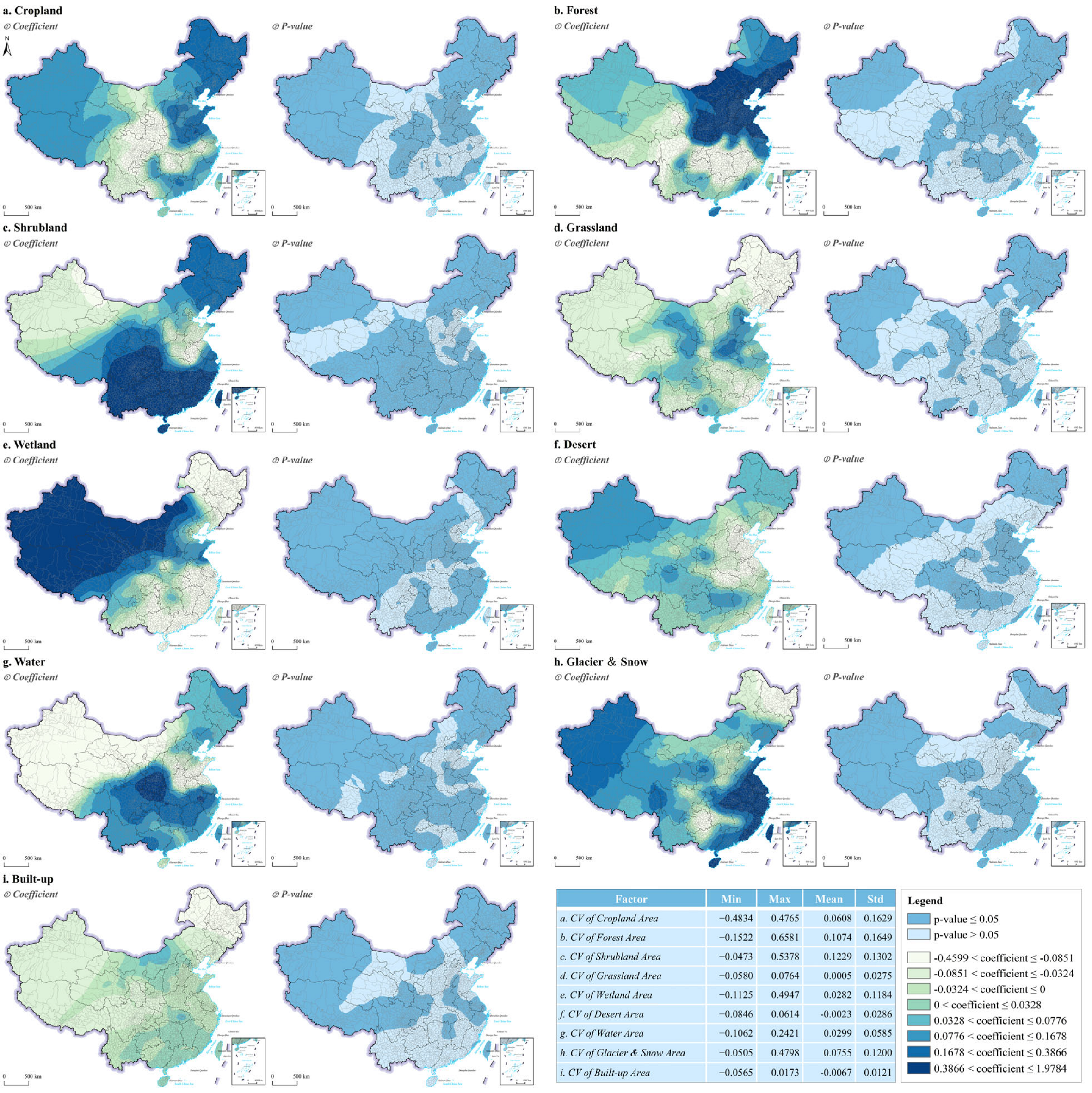
5.3.2. Effects of Area Disagreement in Land Cover Types on the Inconsistency of ESV Evaluations

To further examine the contribution of area discrepancies in specific land cover types to the inconsistency in ESV evaluations, this study employs a geographically weighted regression (GWR) model to investigate the spatially heterogeneous relationships between ESV disagreement and land type area inconsistencies across different datasets. Specifically, the CVs of the areas of nine ecosystem types—calculated from ten land cover datasets—are used as independent variables. In contrast, the CV of ESV estimates serves as the dependent variable. Before applying the GWR model, we conducted a global spatial autocorrelation test (Moran’s I) on the dependent variable to confirm the presence of spatial clustering and the appropriateness of spatial modeling. We adopted an adaptive bandwidth and used the AIC criterion for bandwidth optimization to ensure the spatial scale was appropriate for local estimation. The GWR model performs well, with an R2 of 0.72, indicating a satisfactory level of explanation. In addition, the spatial distribution of local R2 values is provided in the Supplementary Materials (Figure S1), further illustrating the model’s explanatory power across different regions. In Figure 8, panels a1–g1 illustrate the spatial distribution of regression coefficients for the nine ecosystem types, while panels a2–g2 present the corresponding spatial distributions of p-values.
As shown in panels a1–g1 of Figure 8, the regression coefficients representing the influence of area disagreement in different ecosystem types on ESV inconsistency exhibit significant spatial variation across counties. Positive coefficients indicate that inconsistency in the area of a given ecosystem type contributes to increased ESV estimation disagreement in that county. In contrast, negative coefficients suggest a weaker or even offsetting effect. Among the nine ecosystem types, area inconsistency of cropland, forest, shrubland, wetland, and water bodies exhibits the most substantial positive influence on ESV disagreement. For cropland (a1), positive effects are particularly evident in major agricultural regions such as Northeast China, the Huang–Huai–Hai Plain, and South China, where cropland occupies extensive areas. Despite relatively low disagreement in classification and small equivalent factors, even minor inconsistencies in cropland area across datasets can lead to significant variation in ESV estimates. Similarly, for forest (b1), notable positive effects are observed in North China, Northeast China, and coastal regions—areas where forest land is spatially fragmented. This fragmentation increases the sensitivity of ESV estimates to area discrepancies. In contrast, in forest-dominated southern regions, where land cover interpretation tends to be more consistent, area disagreement in forest cover exerts a weaker influence on ESV uncertainty.
The impact of wetland area uncertainty (e1) is particularly pronounced in Northwest China. This region’s spatial extent of wetlands is closely tied to rainfall and water availability. Due to the scarcity and high seasonal variability of water resources, wetlands in this area are prone to substantial interpretation discrepancies among land cover datasets. Given the high equivalent value assigned to wetlands, ESV estimates significantly amplify such discrepancies. Similarly, panel g1 reveals that disagreement in the area of water bodies substantially affects ESV disagreement in southern China. Water ecosystems carry the highest equivalent value among all ecosystem types, and the prevalence of complex water systems in the south means that even minor classification disagreements can result in considerable deviations in ESV estimates. This effect is especially prominent in regions where water bodies contribute to overall ESV. In contrast, panels d1 and i1 show that area disagreement for grassland and built-up land exerts relatively minor effects on ESV inconsistency. This suggests that in these regions, discrepancies in ESVs are not primarily driven by classification inconsistencies in these land types. It also indicates that grassland and urban land, despite potential fluctuations in area estimates, have a limited overall influence on ESV disagreement due to their comparatively lower ecosystem values and more consistent interpretation across datasets.

6. Conclusions

6.1. Findings and Conclusions

This study systematically assessed the uncertainty in county-level ecosystem service value (ESV) evaluations across China using ten widely used land cover datasets. Substantial spatial heterogeneity was observed, with high disagreement concentrated in urbanized and ecologically diverse areas. We quantified dataset-induced differences through statistical indicators such as coefficient of variation and Z-score and identified the most suitable datasets (e.g., CLCD, Globeland30, GLC-FCS30) with higher consistency. Additionally, we investigated the underlying causes of these inconsistencies by analyzing landscape configuration metrics and discrepancies across ecosystem types. We provided targeted recommendations for dataset selection at county and ecological zone levels to support more accurate and sensitive ESV assessments. These contributions provide empirical support for improving the transparency and policy relevance of ESV evaluations.

6.2. Limitations

Despite the comprehensive nature of this analysis, several limitations should be acknowledged. First, the analysis is limited to a single-year snapshot due to the lack of consistent long-term data across all selected products. This limits our ability to analyze temporal dynamics and long-term ESV trends. Second, the average ESV derived from multiple datasets was used as a neutral reference. Although this is a practical and widely accepted approach, it does not represent a validated ground truth value. Third, although the methodological framework developed in this study is broadly applicable, the empirical analysis is geographically restricted to China. The transferability of the findings to other regions remains to be tested, particularly considering the socio-ecological diversity of global contexts. Finally, the attribution analysis primarily focused on differences in land cover classification and spatial configuration. Other potentially important drivers, such as socio-economic factors (e.g., population density, GDP, urban expansion), were not incorporated. Future research should integrate such variables to provide a more comprehensive understanding of the mechanisms driving ESV uncertainty.

Supplementary Materials

The following supporting information can be downloaded at: https://www.mdpi.com/article/10.3390/rs17132320/s1, Table S1: Land cover data products used in this study; Table S2: Reclassification table for different land cover data products; Table S3: The ESV reference values and confidence intervals for each county; Table S4: Comparison of ESV evaluation results across different studies for Wuhan, Lanzhou, and Hangzhou; Figure S1: Spatial Distribution of Local R2 Values from the GWR Model.

Author Contributions

D.S.: methodology, formal analysis, writing—original draft, and visualization; L.W.: investigation, data curation, and writing—original draft; Y.W.: validation, data curation, and formal analysis; B.Z.: investigation and methodology; Q.J.: supervision and project administration; J.Y.: conceptualization, writing—review and editing, supervision, project administration, and funding acquisition. All authors have read and agreed to the published version of the manuscript.

Funding

This study was supported by the National Natural Science Foundation of China (NO.42101275) and the Provincial Natural Science Foundation of Hubei, China (NO.2023AFB651).

Data Availability Statement

The original contributions presented in this study are included in the article/Supplementary Materials. Further inquiries can be directed to the corresponding author.

Acknowledgments

We thank the Center of Big Data and High-Performance Computing in the Department of Land Resources Management at China University of Geosciences (Wuhan), China, for data collection and processing.

Conflicts of Interest

The authors declare no conflicts of interest.

References

  1. Broekx, S.; Liekens, I.; Peelaerts, W.; De Nocker, L.; Landuyt, D.; Staes, J.; Meire, P.; Schaafsma, M.; Van Reeth, W.; Van den Kerckhove, O.; et al. A web application to support the quantification and valuation of ecosystem services. Environ. Impact Assess. Rev. 2013, 40, 65–74. [Google Scholar] [CrossRef]
  2. Baker, J.; Sheate, W.R.; Phillips, P.; Eales, R. Ecosystem services in environmental assessment—Help or hindrance? Environ. Impact Assess. Rev. 2013, 40, 3–13. [Google Scholar] [CrossRef]
  3. Schmidt, S.; Manceur, A.M.; Seppelt, R. Uncertainty of Monetary Valued Ecosystem Services—Value Transfer Functions for Global Mapping. PLoS ONE 2016, 11, e0148524. [Google Scholar] [CrossRef]
  4. Costanza, R. Misconceptions about the valuation of ecosystem services. Ecosyst. Serv. 2024, 70, 101667. [Google Scholar] [CrossRef]
  5. Zhang, Y.; Zheng, M.; Qin, B. Optimization of spatial layout based on ESV-FLUS model from the perspective of Production-Living-Ecological a case study of Wuhan City. Ecol. Model. 2023, 481, 110356. [Google Scholar] [CrossRef]
  6. Chen, Q. Temporal and Spatial Changes of Land Use and Ecosystem Service Value in Wuhan City from 2000 to 2020. Technol. Econ. Chang. 2022, 6, 16–21. [Google Scholar] [CrossRef]
  7. Fu, B.-J.; Su, C.-H.; Wei, Y.-P.; Willett, I.R.; Lü, Y.-H.; Liu, G.-H. Double counting in ecosystem services valuation: Causes and countermeasures. Ecol. Res. 2011, 26, 1–14. [Google Scholar] [CrossRef]
  8. Jacobs, S.; Dendoncker, N.; Martín-López, B.; Barton, D.N.; Gomez-Baggethun, E.; Boeraeve, F.; McGrath, F.L.; Vierikko, K.; Geneletti, D.; Katharina, J.S.; et al. A new valuation school: Integrating diverse values of nature in resource and land use decisions. Ecosyst. Serv. 2016, 22, 213–220. [Google Scholar] [CrossRef]
  9. De Groot, R.; Fisher, B.; Christie, M.; Aronson, J.; Braat, L.; Gowdy, J.; Haines-Young, R.; Maltby, E.; Neuville, A.; Polasky, S.; et al. Integrating the ecological and economic dimensions in biodiversity and ecosystem service valuation. In The Economics of Ecosystems and Biodiversity; Taylor and Francis: London, UK, 2012; pp. 9–40. [Google Scholar]
  10. Costanza, R.; d’Arge, R.; de Groot, R.; Farber, S.; Grasso, M.; Hannon, B.; Limburg, K.; Naeem, S.; O’Neill, R.V.; Paruelo, J.; et al. The value of the world’s ecosystem services and natural capital. Ecol. Econ. 1998, 25, 3–15. [Google Scholar] [CrossRef]
  11. Kumar, P.; Esen, S.E.; Yashiro, M. Linking ecosystem services to strategic environmental assessment in development policies. Environ. Impact Assess. Rev. 2013, 40, 75–81. [Google Scholar] [CrossRef]
  12. de Groot, R.; Brander, L.; van der Ploeg, S.; Costanza, R.; Bernard, F.; Braat, L.; Christie, M.; Crossman, N.; Ghermandi, A.; Hein, L.; et al. Global estimates of the value of ecosystems and their services in monetary units. Ecosyst. Serv. 2012, 1, 50–61. [Google Scholar] [CrossRef]
  13. Davidson, N.C.; van Dam, A.A.; Finlayson, C.M.; McInnes, R.J. Worth of wetlands: Revised global monetary values of coastal and inland wetland ecosystem services. Mar. Freshw. Res. 2019, 70, 1189–1194. [Google Scholar] [CrossRef]
  14. Jiang, W. Mapping ecosystem service value in Germany. Int. J. Sustain. Dev. World Ecol. 2018, 25, 518–534. [Google Scholar] [CrossRef]
  15. Anderson, S.J.; Ankor, B.L.; Sutton, P.C. Ecosystem service valuations of South Africa using a variety of land cover data sources and resolutions. Ecosyst. Serv. 2017, 27, 173–178. [Google Scholar] [CrossRef]
  16. Niquisse, S.; Cabral, P. Assessment of changes in ecosystem service monetary values in Mozambique. Environ. Dev. 2018, 25, 12–22. [Google Scholar] [CrossRef]
  17. Periotto, N.; Tundisi, J. A characterization of ecosystem services, drivers and values of two watersheds in São Paulo State, Brazil. Braz. J. Biol. 2017, 78, 397–407. [Google Scholar] [CrossRef] [PubMed]
  18. Xie, G.; Zhen, L.; Lu, C.; Xia, Y.; Chen, C. Expert Knowledge Based Valuation Method of Ecosystem Services in China. J. Nat. Resour. 2008, 23, 911–919. [Google Scholar]
  19. Xie, G.; Lu, C.; Leng, Y.; Zhen, D.; Li, S. Ecological assets valuation of the Tibetan Plateau. J. Nat. Resour. 2003, 18, 189–196. [Google Scholar]
  20. Zhang, B.; Li, W.; Xie, G. Ecosystem services research in China: Progress and perspective. Ecol. Econ. 2010, 69, 1389–1395. [Google Scholar] [CrossRef]
  21. Kang, N.; Hou, L.; Huang, J.; Liu, H. Ecosystem services valuation in China: A meta-analysis. Sci. Total Environ. 2022, 809, 151122. [Google Scholar] [CrossRef]
  22. Jiang, W.; Wu, T.; Fu, B. The value of ecosystem services in China: A systematic review for twenty years. Ecosyst. Serv. 2021, 52, 101365. [Google Scholar] [CrossRef]
  23. Liu, S.; Costanza, R.; Farber, S.; Troy, A. Valuing ecosystem services: Theory, practice, and the need for a transdisciplinary synthesis. Ann. N. Y. Acad. Sci. 2010, 1185, 54–78. [Google Scholar] [CrossRef]
  24. Zhang, C.; Li, X. Land Use and Land Cover Mapping in the Era of Big Data. Land 2022, 11, 1692. [Google Scholar] [CrossRef]
  25. Karra, K.; Kontgis, C.; Statman-Weil, Z.; Mazzariello, J.C.; Mathis, M.; Brumby, S.P. Global land use/land cover with Sentinel 2 and deep learning. In Proceedings of the 2021 IEEE International Geoscience and Remote Sensing Symposium IGARSS, Brussels, Belgium, 11–16 July 2021; pp. 4704–4707. [Google Scholar]
  26. Buchhorn, M.; Lesiv, M.; Tsendbazar, N.-E.; Herold, M.; Bertels, L.; Smets, B. Copernicus Global Land Cover Layers—Collection 2. Remote Sens. 2020, 12, 1044. [Google Scholar] [CrossRef]
  27. Bicheron, P.; Amberg, V.; Bourg, L.; Petit, D.; Huc, M.; Miras, B.; Brockmann, C.; Hagolle, O.; Delwart, S.; Ranera, F.; et al. Geolocation Assessment of MERIS GlobCover Orthorectified Products. IEEE Trans. Geosci. Remote Sens. 2011, 49, 2972–2982. [Google Scholar] [CrossRef]
  28. ESA. Land Cover CCI. Product User Guide Version 2.0; UCL-Geomatics: London, UK, 2017. [Google Scholar]
  29. Gong, P.; Liu, H.; Zhang, M.; Li, C.; Wang, J.; Huang, H.; Clinton, N.; Ji, L.; Li, W.; Bai, Y.; et al. Stable classification with limited sample: Transferring a 30-m resolution sample set collected in 2015 to mapping 10-m resolution global land cover in 2017. Sci. Bull. 2019, 64, 370–373. [Google Scholar] [CrossRef] [PubMed]
  30. Yang, J.; Huang, X. The 30m annual land cover dataset and its dynamics in China from 1990 to 2019. Earth Syst. Sci. Data 2021, 13, 3907–3925. [Google Scholar] [CrossRef]
  31. Chen, J.; Chen, J.; Liao, A.; Cao, X.; Chen, L.; Chen, X.; He, C.; Han, G.; Peng, S.; Lu, M.; et al. Global land cover mapping at 30m resolution: A POK-based operational approach. J. Photogramm. Remote Sens. 2015, 103, 7–27. [Google Scholar] [CrossRef]
  32. Zhang, X.; Zhao, T.; Xu, H.; Liu, W.; Wang, J.; Chen, X.; Liu, L. GLC_FCS30D: The first global 30 m land-cover dynamics monitoring product with a fine classification system for the period from 1985 to 2022 generated using dense-time-series Landsat imagery and the continuous change-detection method. Earth Syst. Sci. Data 2024, 16, 1353–1381. [Google Scholar] [CrossRef]
  33. Xu, X.; Liu, J.; Zhang, S.; Li, R.; Yan, C.; Wu, S. China’s multi-period land use land cover remote sensing monitoring data set (CNLUCC). [DB/OL]; Data Registration and Publishing System of the Resource and Environment Science Data Center of the Chinese Academy of Sciences: Beijing, China, 2018. [Google Scholar] [CrossRef]
  34. Liu, S.; Wang, H.; Hu, Y.; Zhang, M.; Zhu, Y.; Wang, Z.; Li, D.; Yang, M.; Wang, F. Land Use and Land Cover Mapping in China Using Multimodal Fine-Grained Dual Network. IEEE Trans. Geosci. Remote Sens. 2023, 61, 4405219. [Google Scholar] [CrossRef]
  35. Sulla-Menashe, D.; Gray, J.M.; Abercrombie, S.P.; Friedl, M.A. Hierarchical mapping of annual global land cover 2001 to present: The MODIS Collection 6 Land Cover product. Remote Sens. Environ. 2019, 222, 183–194. [Google Scholar] [CrossRef]
  36. Zanaga, D.; Kerchove, R.V.D.; Keersmaecker, W.d.; Souverijns, N.; Brockmann, C.; Quast, R.; Wevers, J.; Grosu, A.C.; Paccini, A.; Vergnaud, S.; et al. ESA WorldCover 10 m 2020 v100. 2021. Available online: https://pure.iiasa.ac.at/id/eprint/17832/ (accessed on 24 October 2023).
  37. Chakraborty, T.C.; Venter, Z.S.; Demuzere, M.; Zhan, W.; Gao, J.; Zhao, L.; Qian, Y. Large disagreements in estimates of urban land across scales and their implications. Nat. Commun. 2024, 15, 9165. [Google Scholar] [CrossRef] [PubMed]
  38. Congalton, R.G.; Gu, J.; Yadav, K.; Thenkabail, P.; Ozdogan, M. Global Land Cover Mapping: A Review and Uncertainty Analysis. Remote Sens. 2014, 6, 12070–12093. [Google Scholar] [CrossRef]
  39. Bai, Y.; Feng, M.; Jiang, H.; Wang, J.; Zhu, Y.; Liu, Y. Assessing Consistency of Five Global Land Cover Data Sets in China. Remote Sens. 2014, 6, 8739–8759. [Google Scholar] [CrossRef]
  40. Ji, X.; Han, X.; Zhu, X.; Huang, Y.; Song, Z.; Wang, J.; Zhou, M.; Wang, X. Comparison and Validation of Multiple Medium- and High-Resolution Land Cover Products in Southwest China. Remote Sens. 2024, 16, 1111. [Google Scholar] [CrossRef]
  41. Yang, Y.; Xiao, P.; Feng, X.; Li, H. Accuracy assessment of seven global land cover datasets over China. J. Photogramm. Remote Sens. 2017, 125, 156–173. [Google Scholar] [CrossRef]
  42. Fonte, C.C.; Duarte, D.; Jesus, I.; Costa, H.; Benevides, P.; Moreira, F.; Caetano, M. Accuracy Assessment and Comparison of National, European and Global Land Use Land Cover Maps at the National Scale—Case Study: Portugal. Remote Sens. 2024, 16, 1504. [Google Scholar] [CrossRef]
  43. Li, Z.; Chen, X.; Qi, J.; Xu, C.; An, J.; Chen, J. Accuracy assessment of land cover products in China from 2000 to 2020. Sci. Rep. 2023, 13, 12936. [Google Scholar] [CrossRef]
  44. Jiang, J.; Tian, G. Responses of Ecosystem Service Value to Land Use Change in Beijing from 1998 to 2005. Resour. Sci. 2010, 32, 1407–1416. [Google Scholar]
  45. Wang, J.; Hu, Y.; Lv, X.; Zheng, X. Study of Ecosystem Service Values Based on Land Use Change in Beijing. Chin. Agric. Sci. Bull. 2012, 28, 229–236. [Google Scholar]
  46. Li, F.; Zhang, B.; Zhang, S. Ecosystem Service Valuation of Sanjiang Plain. J. Arid. Land Resour. Environ. 2004, 18, 19–23. [Google Scholar]
  47. Wang, Z.; Zhang, S.; Zhang, B. Effects of land use change on values of ecosystem services of Sanjiang Plain, China. China Environ. Sci. 2004, 24, 125–128. [Google Scholar]
  48. Xing, L.; Hu, M.; Wang, Y. Integrating ecosystem services value and uncertainty into regional ecological risk assessment: A case study of Hubei Province, Central China. Sci. Total Environ. 2020, 740, 140126. [Google Scholar] [CrossRef] [PubMed]
  49. Schulp, C.J.E.; Burkhard, B.; Maes, J.; Van Vliet, J.; Verburg, P.H. Uncertainties in Ecosystem Service Maps: A Comparison on the European Scale. PLoS ONE 2014, 9, e109643. [Google Scholar] [CrossRef] [PubMed]
  50. Song, X.-P. Global Estimates of Ecosystem Service Value and Change: Taking Into Account Uncertainties in Satellite-based Land Cover Data. Ecol. Econ. 2018, 143, 227–235. [Google Scholar] [CrossRef]
  51. Zhang, L.; Yu, X.; Jiang, M.; Xue, Z.; Lu, X.; Zou, Y. A consistent ecosystem services valuation method based on Total Economic Value and Equivalent Value Factors: A case study in the Sanjiang Plain, Northeast China. Ecol. Complex. 2017, 29, 40–48. [Google Scholar] [CrossRef]
  52. Herold, M.; Mayaux, P.; Woodcock, C.E.; Baccini, A.; Schmullius, C. Some challenges in global land cover mapping: An assessment of agreement and accuracy in existing 1 km datasets. Remote Sens. Environ. 2008, 112, 2538–2556. [Google Scholar] [CrossRef]
  53. Ouyang, Z. Problems and changing Trends Faced by China’s ecosystem. China Sci. News 2017. [Google Scholar]
  54. Dai, Z.; Hu, Y.; Zhang, Q. Agreement Analysis of Multi-source Land Cover Products Derived from Remote Sensing in South America. Remote Sens. Inf. 2017, 32, 137–148. [Google Scholar]
  55. Xie, G.; Zhang, C.; Zhang, L.; Chen, W.; Li, S. Improvement of the Evaluation Method for Ecosystem Service Value Based on Per Unit Area. J. Nat. Resour. 2015, 30, 1243–1254. [Google Scholar]
  56. Venter, Z.S.; Barton, D.N.; Chakraborty, T.; Simensen, T.; Singh, G. Global 10 m Land Use Land Cover Datasets: A Comparison of Dynamic World, World Cover and Esri Land Cover. Remote Sens. 2022, 14, 4101. [Google Scholar] [CrossRef]
  57. Xu, P.; Tsendbazar, N.-E.; Herold, M.; de Bruin, S.; Koopmans, M.; Birch, T.; Carter, S.; Fritz, S.; Lesiv, M.; Mazur, E.; et al. Comparative validation of recent 10 m-resolution global land cover maps. Remote Sens. Environ. 2024, 311, 114316. [Google Scholar] [CrossRef]
  58. Gao, Y.; Liu, L.; Zhang, X.; Chen, X.; Mi, J.; Xie, S. Consistency Analysis and Accuracy Assessment of Three Global 30-m Land-Cover Products over the European Union using the LUCAS Dataset. Remote Sens. 2020, 12, 3479. [Google Scholar] [CrossRef]
  59. Xu, Y.; Yu, L.; Feng, D.; Peng, D.; Li, C.; Huang, X.; Lu, H.; Gong, P. Comparisons of three recent moderate resolution African land cover datasets: CGLS-LC100, ESA-S2-LC20, and FROM-GLC-Africa30. Int. J. Remote Sens. 2019, 40, 6185–6202. [Google Scholar] [CrossRef]
  60. Zhang, X.; Ren, W.; Peng, H. Urban land use change simulation and spatial responses of ecosystem service value under multiple scenarios: A case study of Wuhan, China. Ecol. Indic. 2022, 144, 109526. [Google Scholar] [CrossRef]
  61. Jiu, J. Study on the Implication of Land Use Change on Ecosystem Service Value in Hubei Province. Master’s Thesis, Huazhong University of Science and Technology, Wuhan, China, 2021. [Google Scholar]
  62. Chen, R.; Huang, C. Landscape Evolution and It’s Impact of Ecosystem Service Value of the Wuhan City, China. Int. J. Environ. Res. Public Health 2021, 18, 13015. [Google Scholar] [CrossRef]
  63. Xiong, X.; Zhou, T.; Cai, T.; Huang, W.; Li, J.; Cui, X.; Li, F. Land Use Transition and Effects on Ecosystem Services in Water-Rich Cities under Rapid Urbanization: A Case Study of Wuhan City, China. Land 2022, 11, 1153. [Google Scholar] [CrossRef]
  64. Cui, X.; Huang, L. Integrating ecosystem services and ecological risks for urban ecological zoning: A case study of Wuhan City, China. Hum. Ecol. Risk Assess. Int. J. 2023, 29, 1299–1317. [Google Scholar] [CrossRef]
  65. Feng, C. Research on Land Use Change and Eeological Risk in LanzhouCity Under Multi-Scenario Simulation. Master’s Thesis, Lanzhou Jiaotong University, Lanzhou, China, 2023. [Google Scholar]
  66. Zou, Y.; Liang, H.; Li, G. Evaluation of ecological carrying capacity and spatial planning strategy based on service function and sensitivity—Taking Lanzhou City as an example. For. Ecol. Sci. 2023, 38, 183–194+208. [Google Scholar] [CrossRef]
  67. Liu, J.; Xiao, B.; Jiao, J.; Li, Y.; Wang, X. Modeling the response of ecological service value to land use change through deep learning simulation in Lanzhou, China. Sci. Total Environ. 2021, 796, 148981. [Google Scholar] [CrossRef]
  68. Wei, Y.; Chen, Q. Study on the evolution of spatial pattern of “three lives” and the response of ecosystem service value: A case study of Hangzhou. In Proceedings of the 2020/2021 China Urban Planning Annual Conference and 2021 China Urban Planning Academic Season, Chengdu, China, 25–30 September 2021; p. 13. [Google Scholar]
  69. Kong, L.; Su, S. Spatiotemporal variation of ecosystem service value in Hangzhou based on land use. Environ. Pollut. Control 2022, 44, 1539–1545. [Google Scholar] [CrossRef]
  70. Li, L. Ecological Risk Assessment of Yangtze River Delta Urban Agglomeration Based on Ecosystem Service Value. Master’s Thesis, Shanghai Normal University, Shanghai, China, 2022. [Google Scholar]
Figure 1. Spatial distribution of ecosystem service value for each county in China, based on ten different land cover datasets (the chart in the bottom right corner presents the proportion of counties falling into different ESV categories for each dataset).
Remotesensing 17 02320 g001
Figure 2. A boxplot analysis of the differences in ESVs for each county in China, based on pairwise comparisons of ten different land cover datasets.
Remotesensing 17 02320 g002
Figure 3. Spatial distribution of reference values of county-level ESVs across China (the reference values were derived as the mean ESV of each county based on assessments using ten different land cover datasets).
Remotesensing 17 02320 g003
Figure 4. (a) Spatial distribution of disagreement in ESV evaluations for each county, based on the coefficient of variation (CV) as a measure of dispersion; (be) the disagreement distribution for the four subtype ecosystem services: provisioning services (b), regulating services (c), supporting services (d), and cultural services (e).
Remotesensing 17 02320 g004
Figure 5. Optimal land cover datasets for ESV evaluation per county in China based on the Z-score method (the dataset corresponding to the smallest Z-score for each county is considered the most suitable, as it indicates the closest ESV estimate to the reference value).
Remotesensing 17 02320 g005
Figure 6. Histograms and kernel density curves that present the distribution of Z-scores for ESV estimates across counties in China for each dataset (the x-axis in the histograms represents equal-width intervals of Z-scores for ESV estimates based on a given dataset, and the y-axis represents the frequency of Z-scores within each interval).
Remotesensing 17 02320 g006
Figure 7. Distribution of ecological function zones and bar chart of dataset recommendation frequencies by zone.
Remotesensing 17 02320 g007
Figure 8. Spatial distribution of coefficients and p-values from the GWR model between ecosystem area uncertainty and ESV estimates uncertainty.
Remotesensing 17 02320 g008
Table 1. Assessment of the applicability of land cover datasets for county-level ESV evaluation in China via mean Z-score and minimum error frequency.
DatasetMean Z-ScoreMinimum Error FrequencyDatasetMean Z-ScoreMinimum Error Frequency
AI Earth0.85.04%ESRI0.88.73%
CGLS_LC1000.6710.56%GLC_FCS300.5612.97%
CLCD0.5115.91%Globeland300.5815.22%
CNLUCC0.939.83%MDC12Q11.233.76%
ESA_CCI0.898.11%World Cover0.719.87%
Table 2. Applicability of different land cover datasets for county-level ESV evaluation in China.
ProportionAI_EarthCGLS_LC100CLCDCNLUCCESA_CCIESRIGLC_FCS30Globeland30MDC12Q1World_Cover
I-01 Water Conservation Functional Zone4.80%8.87%19.33%9.45%5.96%7.12%13.23%20.06%3.63%7.56%
I-02 Biodiversity Conservation Functional Zone4.22%6.17%19.16%11.36%12.99%10.06%9.74%15.26%0.65%10.39%
I-03 Soil Retention Functional Zone2.68%9.75%17.21%11.85%7.46%8.03%17.02%12.43%1.91%11.66%
I-04 Windbreak and Sand Stabilization Functional Zone10.53%11.28%14.29%9.77%9.77%8.27%10.53%13.53%4.51%7.52%
I-05 Flood Regulation Functional Zone11.36%6.82%6.82%11.36%18.18%2.27%9.09%11.36%6.82%15.91%
II-01 Agricultural Production Functional Zone5.99%13.65%13.17%8.98%8.38%9.82%9.70%14.49%5.75%10.06%
II-02 Forestry Production Functional Zone0.00%13.75%16.25%8.75%3.75%1.25%28.75%17.50%3.75%6.25%
III-01 Metropolitan Human Settlement Support Functional Zone2.94%7.84%15.69%6.86%8.82%8.82%16.67%13.73%1.96%16.67%
III-02 Key Urban Cluster Human Settlement Support Functional Zone6.34%9.86%7.75%9.86%7.04%17.61%14.79%10.56%5.63%10.56%
Table 3. Regression analysis between landscape pattern disagreement and ESV evaluation inconsistencies.
VariableUnstandardized Coefficient (B)Standardized Coefficient (Beta)pVIF
Constant−0.3720.000
CV of Patch Density (PD_CV)0.070.140.0002.264
CV of Largest Patch Index (LPI_CV)0.0550.0570.0001.051
CV of Landscape Shape Index (LSI_CV)0.2030.2220.0003.346
CV of Area-Weighted Mean Shape Index (AWMSI_CV)0.280.2760.0002.175
CV of Contagion (CONTAG_CV)0.8620.3780.0001.200
CV of Shannon’s Diversity Index (SHDI_CV)−0.029−0.0280.0971.449
Disclaimer/Publisher’s Note: The statements, opinions and data contained in all publications are solely those of the individual author(s) and contributor(s) and not of MDPI and/or the editor(s). MDPI and/or the editor(s) disclaim responsibility for any injury to people or property resulting from any ideas, methods, instructions or products referred to in the content.

