Impacts of Climate Change on Oceans and Ocean-Based Solutions: A Comprehensive Review from the Deep Learning Perspective

Qiao, Xin; Zhang, Ke; Huang, Weimin

doi:10.3390/rs17132306

Open AccessReview

Impacts of Climate Change on Oceans and Ocean-Based Solutions: A Comprehensive Review from the Deep Learning Perspective

by

Xin Qiao

¹

,

Ke Zhang

² and

Weimin Huang

^1,*

¹

Faculty of Engineering and Applied Science, Memorial University of Newfoundland, St. John’s, NL A1B 3X5, Canada

²

Information Science and Technology College, Dalian Maritime University, Dalian 116026, China

^*

Author to whom correspondence should be addressed.

Remote Sens. 2025, 17(13), 2306; https://doi.org/10.3390/rs17132306

Submission received: 15 April 2025 / Revised: 25 June 2025 / Accepted: 2 July 2025 / Published: 4 July 2025

(This article belongs to the Section Ocean Remote Sensing)

Download

Browse Figures

Versions Notes

Abstract

Climate change poses significant threats to oceans, leading to ocean acidification, sea level rise, and sea ice loss and so on. At the same time, oceans play a crucial role in climate change mitigation and adaptation, offering solutions such as renewable energy and carbon sequestration. Moreover, the availability of diverse ocean data sources, both remote sensing observations and in situ measurements, provides unprecedented opportunities to monitor these processes. Remote sensing data, with its extensive spatial coverage and accessibility, forms the foundation for accurately capturing changes in ocean conditions and developing data-driven solutions. This review explores the dual relationship between climate change and oceans, focusing on the impacts of climate change on oceans and ocean-based strategies to combat these challenges. From the artificial intelligence perspective, this study systematically analyzes recent advances in applying deep learning techniques to understand changes in ocean physical properties and marine ecosystems, as well as to optimize ocean-based climate solutions. By evaluating existing methodologies and identifying knowledge gaps, this review highlights the pivotal role of deep learning in advancing ocean-related climate research, outlines existing current challenges, and provides insights into potential future directions.

Keywords:

climate change; oceans; remote sensing; impacts; solutions; machine learning; deep learning

Graphical Abstract

1. Introduction

Climate change, primarily driven by the emissions of greenhouse gases (GHGs), has led to profound impacts across different ecosystems. In the marine environment, these impacts include ocean warming, acidification, sea-level rise, sea ice loss, and widespread degradation of marine ecosystems such as coral reefs, kelp forests, and coastal wetlands [1,2,3]. These changes not only threaten ocean biodiversity but also compromise the sustainability of coastal communities. On the other hand, ocean-based climate change solutions have emerged as a vital component of global mitigation and adaptation strategies. These include, but are not limited to, advancing marine renewable energy to reduce fossil fuel dependence, optimizing low-carbon maritime transportation, and strengthening coastal ecosystem resilience through monitoring and forecasting. A brief overview of these impacts and corresponding ocean-based solutions is presented in Figure 1.

Understanding the impacts of climate change on oceans and implementing ocean-based solutions rely on large-scale, high-quality ocean data, which serve as the foundation for monitoring changes and predicting trends. These data are obtained from various sources such as satellite remote sensing and in situ measurements. Satellite remote sensing provides large-scale, continuous observations of the ocean surface, enabling global monitoring and long-term trend analysis [4,5]. In contrast, in situ measurements, collected from buoys, vessels, and other instruments, deliver more precise and localized ocean parameters [6]. Extracting meaningful insights from ocean data using advanced analytical models is a crucial step in understanding ocean dynamics and addressing the impacts of climate change. Traditional methods often struggle to process vast and complex datasets, failing to capture intricate relationships within the data. In recent years, artificial intelligence (AI), particularly deep learning (DL) technologies, has emerged as a powerful tool to analyze large-scale datasets, uncover hidden patterns, and produce accurate forecasts [7,8,9]. With these advanced techniques, researchers can better understand the impacts of climate change on oceans and develop more effective solutions to mitigate its effects and enhance resilience.

While DL has been increasingly applied to the above-mentioned ocean-related research, a comprehensive review that integrates DL architectures, data sources, application domains, and core methodological challenges is still lacking. To fill this gap, this review synthesizes recent advances in applying DL to both the impacts of climate change on the oceans and ocean-based climate solutions, aiming to address the following key questions:

Which DL architectures demonstrate high performance for different types of oceanography problems?
Which physical processes in the ocean are poorly modeled by existing DL approaches and why?
How do different types of oceanography data (satellite, in situ, reanalysis) affect the performance of DL models?
How is the problem of different spatiotemporal resolutions in multisensory data (satellite observations) addressed?

The remainder of this review is organized as follows. Section 2 introduces the major types of ocean data, including observational data, model data, and reanalysis data. This section also discusses how these data types differ in terms of spatial and temporal resolution, and outlines common strategies to address the challenge of heterogeneous spatiotemporal resolutions in multisensory data. Section 3 summarizes the deep learning models commonly adopted in ocean studies. Section 4 explores DL applications in analyzing the impacts of climate change on oceans and Section 5 discusses DL-based strategies to support ocean-based climate change solutions, highlighting commonly used DL architectures and evaluating their performance for different types of oceanography problems. Finally, Section 6 presents a conclusive synthesis, identifies key challenges like ocean physical processes that are poorly modeled by existing DL approaches, and outlines future research directions.

2. Data: Foundations of Ocean Studies

Ocean data are essential for monitoring ocean changes, forecasting future conditions, and developing effective mitigation strategies [10]. Because they originate from multiple sources and serve diverse purposes, these data can be classified according to different criteria, such as data source, application areas, or inherent characteristics. In this review, ocean data are grouped into three main categories, including observational data, model data, and reanalysis data. Table 1 offers a comprehensive summary of these categories and the following subsections provide a more detailed discussion for each type.

2.1. Observational Data

Observational data refers to information collected directly through instrument measurement and can be further categorized into remote sensing data and in situ observation data, depending on whether instruments observe ocean parameters from a distance or directly within the water column [11]. This section presents an overview of both categories, focusing on commonly used data sources, resolutions, and their applications in ocean studies.

2.1.1. Remote Sensing Data

Remote sensing captures ocean properties from a distance using sensors mounted on satellites, aerial platforms, land, or ships, without direct physical contact [12,13]. These sensors operate across various parts of the electromagnetic spectrum, ranging from optical frequencies to radio waves.

Optical Remote Sensing

Optical remote sensing measures electromagnetic radiation in the visible (roughly 0.4 µm to 0.7 µm) and infrared (about 0.7 µm to 1 mm) bands. Common instruments for optical remote sensing include Moderate Resolution Imaging Spectroradiometer (MODIS), Visible Infrared Imaging Radiometer Suite (VIIRS), Ocean and Land Color Instrument (OLCI) [14,15], and Geostationary Ocean Color Imager (GOCI), which is the first geostationary ocean color sensor and provides observations essential for monitoring coastal water dynamics, sea ice, and primary productivity [16,17,18]. These sensors record reflectance characteristics of the ocean surface and produce multispectral images (MSIs), which provide critical information on ocean properties such as sea ice extent, chlorophyll concentration, and coastal habitats. Moreover, PlanetScope, a satellite constellation operated by Planet Labs and comprising over 130 CubeSats, captures imagery in eight spectral bands at a spatial resolution of 3–5 m per pixel. It has been widely used in coastal applications, such as wetland monitoring and Sargassum inundation detection [19]. By leveraging these data, optical remote sensing enables comprehensive monitoring of marine environments and their dynamics [20,21].

A key limitation of optical remote sensing is its dependence on clear atmospheric conditions and adequate sunlight for data acquisition [22]. Factors such as cloud cover, aerosols, and water vapor can obstruct light propagation, reducing data quality and availability. In addition, the absence of sunlight during nighttime or polar winters further limits the frequency and consistency of data collection, posing challenges for continuous ocean observation.

SAR

Microwave remote sensing exploits longer wavelengths (1 mm to 1 m) to penetrate clouds, rain, and fog, enabling all-weather and day or night observations. Among various microwave techniques, Synthetic Aperture Radar (SAR) stands out for its ability to produce high-resolution images of the ocean surface [23]. Commonly used SAR systems include Sentinel-1, RADARSAT, and GaoFen-3 (GF-3) [24,25,26]. Sentinel-1, developed by the European Space Agency (ESA), is a radar imaging system initially comprising two satellites, Sentinel-1A and Sentinel-1B, both equipped with C-band SAR sensors. Following the termination of Sentinel-1B in 2022, Sentinel-1C was launched in December 2024 to ensure the continuity of the mission. The RADARSAT program, led by the Canadian Space Agency, includes RADARSAT-2 (launched in 2007) and the RADARSAT Constellation Mission (RCM, launched in 2019), enabling all-weather imaging for applications such as sea ice mapping and ship detection. TerraSAR-X is another widely used SAR mission for sea state monitoring [27]. GF-3, a Chinese satellite launched in 2016, is equipped with C-band SAR systems, offering high-resolution images [28]. These systems are widely used for various applications such as monitoring sea ice, detecting oil spills, observing coastal dynamics, and tracking ocean waves or currents [29]. In addition, the ICEYE satellite constellation consists of over 25 microsatellites equipped with SAR operating at X-band frequencies, enabling all-weather, day-and-night Earth observation with high spatial resolution (e.g., 25 cm–1 m at dwell imaging modes). These data have been used in applications such as flood monitoring [30] and oil spill detection [31].

GNSS-R

In contrast to Synthetic Aperture Radar (SAR), which actively emits signals, Global Navigation Satellite System Reflectometry (GNSS-R) has emerged as a novel passive remote sensing technology utilizing signals from existing GNSS constellations like Global Positioning System [32,33]. These signals are transmitted by GNSS satellites, reflected from the ocean surface, and then captured by a GNSS-R receiver. By analyzing the reflected signals and the direct signals, GNSS-R enables the retrieval of ocean parameters such as wind speed and wave height, achieving sea surface measurement at a lower cost compared to active radar systems.

TechDemoSat-1 (TDS-1) was one of the pioneering satellite missions to demonstrate the feasibility of employing GNSS-R for Earth observation and has been successfully used for monitoring sea ice coverage, estimating sea ice thickness, and determining sea ice concentration [34,35]. Building on the success of TDS-1, the Cyclone Global Navigation Satellite System (CYGNSS) was launched in 2016 by the National Aeronautics and Space Administration (NASA). CYGNSS, originally designed for sea surface wind and tropical cyclone monitoring, has been expanded to broader ocean studies such as wave height estimation and oil spill detection, showcasing the versatility of GNSS-R technology [36,37].

Passive Microwave

Passive microwave remote sensing detects naturally emitted microwave radiation from the Earth’s surface. Compared to optical sensors, passive microwave radiometers are much less affected by cloud cover and atmospheric aerosols, making them particularly valuable for continuous monitoring of ocean surface conditions under all weather and illumination conditions. Sensors such as the Advanced Microwave Scanning Radiometer 2 (AMSR-2), onboard the Global Change Observation Mission—Water satellite, operate across a broad range of frequency channels (e.g., 6.9 to 89 GHz) and enable the retrieval of key oceanographic parameters, including sea surface temperature, sea ice concentration, and surface wind speed [38,39]. These observations play a critical role in climate monitoring, numerical weather prediction, and operational oceanography.

LiDAR

Light Detection and Ranging (LiDAR) is an active remote sensing technology that uses laser pulses to measure ocean targets with exceptional precision. By emitting laser light and analyzing the return signals, LiDAR generates detailed information about the ocean surface [40]. A notable example is the ICESat-2 satellite, which utilizes the Advanced Topographic Laser Altimeter System (ATLAS) to measure ice sheet elevations, track changes in sea ice, and monitor surface water levels with remarkable accuracy [41].

X-Band Radar

X-band marine radars operate within the frequency range of 8–12 GHz, with a wavelength of around 3 cm, delivering high spatial resolution in applications like wave monitoring and current measurements [42]. Commonly installed on ships or coastal stations, these radar systems provide real-time assessments of ocean dynamics, making them valuable for ocean observation and maritime operations [43].

HF Radar

Moving to even longer wavelengths, high-frequency (HF) radar systems operate at wavelengths of 10–100 m and are widely used for nearshore currents and wave measurements [44]. For instance, the National Oceanic and Atmospheric Administration (NOAA) Integrated Ocean Observing System HF Radar network offers real-time monitoring of coastal currents along the U.S. coastline, providing critical information for coastal management. Although HF radar excels in large-scale, continuous observations, its main drawback is lower spatial resolution compared to optical and X-band marine radar systems.

Acoustic Remote Sensing

In addition to electromagnetic waves, acoustic remote sensing is another vital method for ocean data acquisition [45]. Acoustic remote sensing utilizes sound waves to investigate situations below the ocean surface, offering significant advantages over electromagnetic waves due to their efficient propagation through water. Common instruments in acoustic remote sensing include single-beam and multibeam echo sounders, side-scan sonar, and acoustic Doppler current profilers. These tools can generate high-resolution ocean floor maps, detect fisheries, and offer valuable insights into underwater environments [46,47].

2.1.2. In Situ Observation Data

In situ observation data are collected directly from the ocean using a variety of instruments deployed in the water, providing highly accurate and localized measurements. These instruments include buoys, floats, underwater cameras, tide gauges, and research vessels, each offering unique capabilities [48]. Specifically, buoys, such as those operated by the National Data Buoy Center (NDBC), are stationary platforms equipped with sensors to measure wave height, SST, and atmospheric pressure, providing insights into oceanographic and meteorological processes [49]. Floats, such as Argo floats, are free-drifting devices that move vertically through the water column, gathering data on temperature, salinity, and other ocean parameters at varying depths to support studies on ocean circulation, ecosystem dynamics, and climate-driven changes. Underwater cameras capture visual data on marine ecosystems and biodiversity, offering direct observations of subsurface habitats [50]. Tide gauges, positioned along coastlines, monitor changes in sea level and tidal patterns, contributing to research on coastal dynamics and sea level rise. Research vessels play a vital role in in situ ocean observation by offering high-resolution, multiparameter measurements [51]. Equipped with advanced instruments such as Conductivity-Temperature-Depth profilers and rosette samplers, these ships can collect detailed data on physical (e.g., temperature, salinity), chemical (e.g., dissolved oxygen, pH), and biological (e.g., chlorophyll concentration, plankton abundance) parameters. Unlike autonomous platforms such as buoys or floats, research vessels allow adaptive mission planning and direct human supervision, valuable for validating satellite observations and supporting interdisciplinary research. Notable programs include the Global Ocean Data Analysis Project (GLODAP), which provides high-quality, ship-based measurements of the ocean carbon system, and the Global Ocean Ship-based Hydrographic Investigations Program (GO-SHIP), which offers physical and biogeochemical ocean data to support global climate research.

While ocean remote sensing provides broader spatial coverage, in situ observation data complement it by delivering ground-truth measurements that validate remote observations, improving the accuracy and reliability of oceanographic information.

2.2. Model Data

Observational data, including remote sensing and in situ measurements, capture real-time or historical ocean conditions, whereas model data simulate or forecast ocean states under given physical, chemical, and biological processes. These numerical models use mathematical frameworks such as partial differential equations or machine learning algorithms, to represent ocean dynamics, including currents, temperature distribution, and other variables, across various spatial and temporal scales. Common modeling frameworks in ocean climate change fields include the Coupled Model Intercomparison Project (CMIP), WaveWatch III (WW3), and GraphCast [52,53]. CMIP orchestrates multimodel comparisons and standardized simulations to advance the understanding of climate projections and inter-model variability. WW3 is a third-generation wave model developed by NOAA to simulate and forecast global ocean waves by solving the spectral action balance equation and accounting for key physical processes such as wave generation, propagation, and dissipation. It can also assimilate data from other sources, such as satellite observations or in situ buoy measurements. GraphCast, on the other hand, is a DL-based forecast framework that leverages large datasets and AI algorithms to predict ocean and atmospheric conditions, offering an alternative to traditional physics-based models [54].

Model data fill gaps in observational coverage by providing consistent, high-resolution information on variables such as sea surface height (SSH), temperature, and pressure over a specific region and period. However, model outputs may deviate from reality due to uncertainties in parameterizations, boundary conditions, and initial states. To address these challenges, continuous advancements in modeling and the incorporation of more sophisticated data assimilation techniques help mitigate these issues by anchoring simulations in real-world measurements, as described in Section 2.3.

2.3. Reanalysis Data

Reanalysis data combines observational data with numerical model outputs using advanced data assimilation techniques to produce gridded ocean datasets [55,56]. By regularly correcting models with newly ingested measurements, reanalysis data minimizes discrepancies between simulations and reality, ensuring more accurate and reliable results. These data products are essential resources for studying large-scale ocean dynamics, climate trends, and long-term variability. Several widely used reanalysis datasets include:

ERA5: The fifth-generation reanalysis dataset from the European Centre for Medium-Range Weather Forecasts (ECMWF), known as ERA5, integrates satellite observations, in situ measurements, and numerical model analyses to produce high-quality datasets [57]. ERA5 offers data at varying spatial and temporal resolutions, such as sea surface wind speed at 0.25 $°$ resolution and wave height at 0.5 $°$ resolution, with an hourly time step [58,59]. This comprehensive dataset supports a wide range of applications in meteorology, oceanography, and climate research.
SODA: The Simple Ocean Data Assimilation (SODA) dataset, developed by the University of Maryland, combines historical satellite observations, buoy data, ship-based measurements, and other observations with physical ocean models, providing high-resolution, three-dimensional representations of ocean states. This dataset is widely used for studying long-term oceanographic changes and validating global climate models [60].
GODAS: Produced by the U.S. National Centers for Environmental Prediction, Global Ocean Data Assimilation System (GODAS) integrates observational data with numerical models to generate high-resolution gridded datasets of oceanic variables, such as temperature, salinity, and current [61]. This reanalysis data focus on seasonal forecasting, especially the prediction of El Niño-Southern Oscillation (ENSO), making it a crucial tool for climate research and weather prediction [62].
OISST: The Optimum Interpolation Sea Surface Temperature (OISST) dataset, provided by the U.S. National Centers for Environmental Information (NCEI), integrates in situ observations with satellite measurements and applies an interpolation algorithm to create consistent, gap-filled SST fields. These datasets are essential for analyzing SST trends, monitoring marine heatwaves (MHWs), and supporting climate predictions [63,64].
GLORYS: Developed by the European Copernicus Marine Environment Monitoring Service (CMEMS), Global Ocean Reanalysis and Simulation (GLORYS) reanalysis products provide global datasets with a high spatial resolution of 1/12 $°$ (approximately 8 km). These datasets include variables for currents, sea level, temperature, salinity, mixed layer depth, and ice parameters, making them valuable for oceanographic and climate studies [65].

Different types of oceanographic datasets, such as satellite remote sensing, in situ observations, and reanalysis products, are suitable for different DL tasks. For example, satellite remote sensing data are ideal for tasks that require broad spatial coverage and frequent observations, such as SST prediction and sea ice classification. In situ observations are well suited for ocean surface pH estimation, and reanalysis data are commonly used in global-scale studies and long-term forecasting tasks, such as global sea surface wind speed and wave height estimation. Different data sources also bring distinct advantages and limitations that affect the accuracies and generalizations of DL models. For example, satellite data offer broad spatial coverage, which enables DL models to capture large-scale oceanographic patterns. However, sensors like MODIS suffer from missing values due to cloud cover or atmospheric interference, which can degrade model performance, especially for fine-resolution classification or detection. In situ data provide high-accuracy point measurements, but their limited spatial coverage and irregular sampling can lead to data sparsity, which may lead to overfitting and affect the generalization capabilities of DL models. Reanalysis data provide full spatial and temporal coverage and are widely used as labels for DL model training. However, since these datasets are generated through data assimilation, they may introduce systematic biases and over-smoothing, especially in extreme conditions. For instance, ERA5, one of the most widely used reanalysis products, inherently lacks high wind speed measurements. As a result, DL models trained on ERA5 wind speed data may underestimate high wind speeds, limiting their effectiveness in applications such as storm forecasting.

Ocean data exhibits different data quality issues such as missing values, spatiotemporal heterogeneity, and calibration issues. Missing values refer to absent or invalid observations in oceanographic datasets, resulting from factors such as cloud cover and sensor malfunction. Properly handling missing values is essential in DL, as most DL frameworks cannot process NaN values directly, leading to errors during forward or backward propagation. A common approach to deal with missing data is data imputation, where missing values are substituted with statistical estimates, such as the mean, median, or interpolated values [66]. In more advanced DL architectures, such as masked autoencoders (MAEs), masking mechanisms can be employed to selectively ignore missing parts of the input data and focus on valid observations, as demonstrated in recent applications such as SST gap filling under cloud-covered conditions [67].

Spatiotemporal heterogeneity refers to the inconsistent spatial and temporal resolutions among different oceanographic datasets, which can come across different sensors or the same sensor with varying acquisition modes. For example, MODIS provides 250 m, 500 m, and 1 km products, while Sentinel-2 offers 10 m, 20 m, and 60 m data. To address spatial inconsistencies, interpolation and resampling techniques are widely used, where lower-resolution data are upsampled to match higher-resolution data. For example, MODIS data are upsampled to 30 m to align with Landsat images for fine-scale analysis [68], and ERA5 wind speeds are interpolated to match the geolocation of CYGNSS observations for training DL-based wind retrieval models [69]. DL-based super-resolution models can be employed to enhance the spatial resolution of coarse data, enabling more detailed feature extraction and improving model performance in tasks such as SST monitoring [70,71]. Moreover, temporal mismatches are typically addressed through temporal interpolation (e.g., linear, spline) or temporal aggregation (e.g., daily, monthly averages) [72], enabling alignment across different temporal resolutions.

Calibration issues mean that an instrument’s measurements deviate from the actual values. These issues can arise from various factors, such as environmental influences, instrument degradation or replacement, and procedural errors in the calibration process. For example, a recent study identified a systematic bias in wind speed measurements from the Tropical Atmosphere Ocean buoy array due to changes in anemometer types [73]. Such biases may lead DL models to learn inaccurate patterns from the data and generate unreliable results. To mitigate calibration-related challenges, cross-sensor calibration is often employed. This process involves comparing and adjusting data from multiple sensors to ensure consistency and reliability across different instruments. For example, simultaneous nadir overpass (SNO) is a commonly used approach for calibrating multiple satellite sensors. SNO refers to the condition where two satellites observe the same geographic location at nearly the same time and from similar near-nadir viewing angles. Because the observation conditions are highly consistent, the measurements from both sensors can be directly compared to identify and correct systematic biases, improving cross-sensor consistency. In [74], Barnes et al. conducted a cross-calibration of the long near-infrared bands between MODIS and VIIRS. By identifying matched observations with similar viewing and illumination geometry, they calculated radiance ratios to quantify sensor differences and adjust VIIRS measurements, leading to improved consistency in downstream ocean color products such as chlorophyll-a concentration.

Figure 2 displays several examples of the aforementioned data, and Table 1 provides a comprehensive summary of ocean data, including their sources, characteristics, and typical applications in ocean research. It is worth noting that while several remote sensing datasets, such as Sentinel-1 SAR, are accessible on platforms like Google Earth Engine (GEE) [75,76], others, like in situ buoy data, are not included. As a result, understanding the original data sources becomes crucial for fully utilizing these datasets. Ocean data, encompassing observational, model, and reanalysis data, form the foundation for understanding and addressing ocean and climate-related challenges. Observational data provide real-time measurements while model and reanalysis data offer large-scale, consistent information. Together, these datasets support comprehensive analyses of the changes in ocean and climate.

3. DL Models for Ocean Studies

The expanding volume and complexity of ocean data require advanced analytical techniques for meaningful insights extraction. ML methods such as random forest (RF) have been widely used for ocean data analysis [77,78]. RF is an ensemble learning method that constructs multiple decision trees and combines their outputs to improve robustness and generalization [79]. While these traditional ML methods are effective, DL, a subset of machine learning, has emerged as a powerful tool to identify intricate relationships from high-dimensional ocean data [80]. By automatically learning complex feature representations, DL models can effectively process large-scale, multimodal ocean data and significantly improve the accuracy for both descriptive and predictive tasks. This section summarizes six commonly used neural network architectures, as depicted in Figure 3, illustrating their fundamental structures and typical applications in ocean studies.

3.1. MLP

The Multilayer Perceptron (MLP) represents one of the most foundational neural network designs. It typically consists of an input layer, one or more hidden layers, and an output layer, with each neuron in a given layer fully connected to every neuron in the next. During training, the model adjusts its learnable weights to minimize prediction errors, while nonlinear activation functions such as Rectified Linear Unit (ReLU) enable the MLP to capture complex, nonlinear patterns in the input data. In ocean-related research, MLPs are well suited for analyzing tabular data, modeling relationships among environmental variables (e.g., temperature, salinity, pH), and making predictions based on sensor inputs [81]. Their relatively simple structure also ensures computational efficiency and ease of implementation.

3.2. Convolution-Based Architecture

3.2.1. Vanilla CNNs

Vanilla CNNs are a kind of DL model specifically designed for image processing tasks, making them highly effective for ocean remote sensing applications, such as sea ice classification, sea surface wind estimation, and chlorophyll concentration estimation [82]. A typical CNN architecture includes convolutional layers, activation functions, pooling layers, and fully connected layers. Convolutional kernels slide over the input data, such as satellite or underwater camera images, extracting spatial features like edges and textures, while activation functions like ReLU and Leaky ReLU introduce nonlinearity. Pooling layers, including max pooling and average pooling, reduce the spatial dimension of feature maps to alleviate computational overhead. Batch normalization and dropout further stabilize the training process and prevent overfitting [83].

3.2.2. U-Net

U-Net is widely used for image segmentation tasks, especially for remote sensing images [84]. It follows an encoder–decoder structure in which the encoder progressively downsamples the input image to capture high-level features, while the decoder upsamples to reconstruct spatial resolution. Another characteristic of U-Net lies in its skip connections, which transfer fine-grained features from the encoder to the corresponding decoder layers, contributing to producing accurate segmentation results. U-Net is well suited for sea ice, coastal habitats, or coral reef monitoring. By segmenting complex remote sensing imagery at high accuracy, U-Net provides valuable insights for marine ecosystem monitoring and climate change assessments [8].

3.3. RNN

Many oceanographic applications involve time-series data and RNNs are specifically designed for temporal dependencies extraction through recurrent connections. Gated Recurrent Unit (GRU) and Long Short-Term Memory (LSTM) are two notable variants that incorporate gating mechanisms to regulate information flows across time steps [85]. These mechanisms allow the model to selectively retain or discard information, making them effective at capturing long-term dependencies in complex time-series data. In the context of ocean climate change, RNNs facilitate the analysis of historical trends, valuable for temperature, wind speed, or wave height prediction [86].

3.4. GAN

Generative Adversarial Networks (GANs) comprise two neural networks: a generator, which generates synthetic samples resembling real data, and a discriminator, which distinguishes between real and synthetic inputs. These two networks are trained simultaneously through an adversarial strategy, where the generator strives to create increasingly realistic data, and the discriminator aims to improve its ability to differentiate between real and fake samples. This dynamic competition prompts both networks to enhance their performance, generating highly realistic synthetic data. In ocean studies, GANs have been successfully employed to enhance training sample diversity by data augmentation, generate synthetic imagery to fill gaps caused by cloud cover or sensor malfunctions [87], and improve the spatial resolution of satellite data for refined observation [88,89].

3.5. ViT

Originally designed for natural language processing, the Transformer architecture has been adapted to computer vision tasks in the form of the Vision Transformer (ViT). A typical ViT follows a structured process involving several key steps. First, the input image is divided into smaller patches, which are embedded into a sequence through a patch embedding layer. Next, the embedded patches are processed by a series of Transformer encoder layers, where self-attention mechanisms are applied to capture global dependencies across the entire image. Finally, the output from the encoder layers is passed through a classification head to generate the final prediction. In contrast to CNNs, which focus on local feature extraction, ViTs can directly model the global context. This global perspective proves to be advantageous in large-scale ocean remote sensing tasks, such as SST or MHV predictions, and sea ice classification [90,91].

The aforementioned models exhibit varying strengths across tasks like classification, segmentation, and time-series forecasting. MLPs are well suited for tasks involving structured tabular data, such as estimating ocean surface pH from variables like SST, sea surface salinity (SSS), and dissolved inorganic carbon (DIC). However, they lack the ability to model spatial or temporal dependencies, and thus, they are not suitable for processing high-dimensional gridded data (e.g., satellite imagery) or time series data. CNN-based architectures like Vanilla CNNs and U-Nets are widely used for spatial classification and segmentation tasks, such as sea ice classification, coral reef or kelp mapping, and coastal wetland monitoring, due to their ability to capture spatial features from gridded remote sensing images. However, these models are inherently limited by their local receptive fields, making it difficult to capture long-range spatial dependencies or global relationships. Besides, conventional CNNs cannot capture temporal information and often require integration with temporal modules such as LSTM. As a result, standalone CNN models are less suitable for applications involving temporal forecasting (e.g., sea level prediction) or for processing nongrid structured data (e.g., tabular in situ buoy observations). Tasks involving temporal forecasting, like SST and ENSO prediction, ship fuel consumption forecasting, and wind speed estimation, are beneficial from sequence models like GRU, LSTM, and TCN, which are effective in capturing sequential dependencies. Among them, LSTMs leverage gating mechanisms to retain long-term memory more effectively than traditional RNNs, enabling them to predict SST with lead times of up to 18 months. However, these models are inherently limited in capturing spatial structures and are often integrated with CNNs to model spatiotemporal patterns. Transformers and their variants, such as Vision Transformers, have demonstrated superior performance in complex spatiotemporal tasks due to their powerful self-attention mechanism, which allows the model to dynamically focus on relevant features across time and space. Despite these advantages, Transformer-based models often require high computational resources and large volumes of high-quality data, making them suitable for tasks involving abundant spatiotemporal datasets and less effective in applications with limited training samples. Several representative DL architectures applied to various oceanographic tasks are summarized in Table 2, Table 3 and Table 4, which report quantitative performance metrics such as accuracy, RMSE, and correlation coefficients. These analyses aim to provide some insights for researchers in selecting DL architectures based on the characteristics of their datasets and specific tasks.

In addition to these commonly used models, other advanced architectures, such as Graph Neural Networks (GNNs), also play important roles in ocean-related studies [92]. Unlike CNNs, which require regularly gridded input data, GNNs can flexibly represent observations as graphs, where nodes correspond to observation points and edges incorporate spatial proximity or learned relationships [93]. This flexibility makes GNNs well suited for irregular spatial data processing, and they have been successfully applied to various ocean-related tasks, such as modeling large-scale ocean circulation and forecasting SST or MHWs [94,95]. For instance, researchers have modeled SST as spatiotemporal graphs [96], where each node represents an observation point defined by a specific latitude and longitude. The node features consist of historical SST time series and other auxiliary variables, such as wind speed or atmospheric pressure, capturing the temporal evolution of the local environment. The edges encode spatial relationships between nodes, such as geographical proximity or physical connectivity. This graph-based network allows the model to leverage the structural information of a graph, which is beneficial for capturing spatial dependencies and modeling regional interactions.

In practice, researchers often combine multiple architectures to harness their complementary capabilities; for example, coupling a CNN with an RNN to extract spatial patterns and temporal dependencies simultaneously [97] or incorporating Transformers alongside CNNs for hybrid local-global feature extraction. Such integrated approaches can provide more robust and accurate models to tackle complex ocean and climate change challenges.

4. Impact of Climate Change on Oceans: Leveraging DL for Monitoring and Analysis

Climate change has generated profound impacts on oceans, driving shifts in physical properties and posing threats to marine ecosystems. DL techniques provide transformative tools to investigate these impacts. This section examines how DL models are applied to analyze changes in physical ocean parameters and monitor various vulnerable marine ecosystems.

4.1. Understanding Impacts on Physical Properties via DL

Physical changes include variations in ocean pH, SST, sea ice extent, and sea level. This subsection explores the application of DL models in analyzing these changes, highlighting the commonly used datasets and models for each specific task, as depicted in Figure 4 and Table 2.

4.1.1. Applying DL to Estimate Ocean pH Levels

Ocean acidification refers to the ongoing decrease in ocean pH levels caused by the absorption of excess anthropogenic CO₂ from the atmosphere. Dissolved CO₂ in seawater forms carbonic acid, which dissociates into hydrogen ions, increasing ocean acidity and lowering pH. A recent study by Ma et al. [98] analyzed four decades of global surface ocean acidification (1982–2021), revealing a declining rate of −0.0166 ± 0.0010 per decade. This study also highlighted significant regional variability, with high-latitude regions, such as the Arctic, experiencing the fastest acidification rates.

Accurate monitoring of ocean pH is crucial for understanding acidification trends and mitigating their impacts. However, traditional in situ sensors are costly and limited in spatial and temporal coverage. To address this limitation, data-driven approaches have been increasingly applied to estimate ocean pH levels from different environmental variables. Recent studies have employed ML and DL techniques, such as RF, feedforward neural networks (FFNNs) [99,100], and the Back Propagation neural network (BP-NN) [101], to map pH distributions with high spatial and temporal resolution by integrating satellite-derived SST, chlorophyll-a concentration, dissolved oxygen, and other in situ observations [102]. These methods have demonstrated strong agreement with reference data, validating their effectiveness for large-scale ocean acidification monitoring [103,104]. It should be noted that direct measurement of ocean surface pH from space is not possible. Instead, all current approaches rely on indirect estimation, where pH is inferred using models trained on in situ pH measurements and other associated surface variables such as SST, SSS, pCO₂, and chlorophyll concentrations. Some of these variables, like SST and chlorophyll concentration, are retrievable from satellite observations.

In addition to pH levels, DL has also been leveraged to estimate total alkalinity (TA) [105], which is a key variable in assessing ocean buffer capability, i.e., its ability to resist changes in pH when absorbing CO₂. Models such as Artificial Neural Network (ANN) [106] and TabNet [107] have shown promising accuracy in estimating global TA distributions from remote sensing inputs and in situ measurements [108], further highlighting the potential of advanced DL techniques in capturing TA variations and enhancing our understanding of ocean acidification [109,110].

4.1.2. DL for Predicting Ocean Warming Trends and Associated Extreme Weather Events

As global temperatures rise, oceans absorb excess heat from the atmosphere, leading to an increase in SST, known as ocean warming [111]. This process has significant consequences, including threatening marine biodiversity, rising sea levels, and intensifying extreme weather events. Analyzing historical SST patterns and forecasting future trends require robust analytical methods, with DL proving to be a highly effective approach.

DL models, such as CNNs and RNNs, offer significant advantages in capturing spatial and temporal features, making them powerful tools for SST prediction [112]. Yu et al. [113] proposed a GRU-CNN hybrid model to integrate temporal and spatial information for accurate SST prediction. Using OISST data specific to the East China Sea and the Yellow Sea, the model demonstrated superior performance, achieving high accuracy across forecasting horizons ranging from 3 days to 1 month, highlighting its robustness and strong predictive capabilities. Xie et al. [114] introduced attention mechanisms in GRU models to adaptively assign weights for key time steps, further improving SST prediction accuracy. In addition to GRU, models combining LSTM with CNNs, known as ConvLSTM architectures, are also widely used for SST prediction due to their ability to effectively capture both temporal dependencies and spatial features. Both Xiao et al. [115] and Hou et al. [116] utilized ConvLSTM for SST forecasting, with Xiao et al. further enhancing the model by incorporating dilation convolutional kernels. This modification enabled the model to capture varying spatial scales, significantly improving its ability to learn multiscale spatial features.

Beyond CNNs and RNNs, other architectures like U-Net and Transformers have also been explored for SST prediction, offering exceptional capabilities in capturing spatial and temporal features. U-Net, a specialized model with an encoder–decoder structure, is particularly effective for spatial feature extraction in SST forecasting. Qi et al. [117] introduced a 3D U-Net model that integrates both spatial and temporal information, outperforming ConvLSTM models with smaller prediction errors across all forecasting periods. Similarly, Taylor et al. [118] combined U-Net and LSTM architectures to predict global SSTs up to 24 months in advance. Using ERA5 monthly mean SST data and 2 m air temperature data from 1950 to 2021, their model demonstrated high accuracy, particularly in the equatorial and subtropical Pacific regions. Transformers, on the other hand, are effective for time-series modeling and well suited for long-term SST prediction. Dai et al. [119] introduced a Transformer-based model specifically designed for fine-grained daily SST forecasting. The model incorporated temporal embedding, attention distillation, and partial stacked connections to enhance performance. Using OISST data from September 1981 to 2023, the model achieved accurate forecasts for up to 360 days across five regions in the China Sea, outperforming existing methods and highlighting the significant potential of Transformers for reliable, long-term SST prediction.

In addition to SST prediction, deep neural networks have shown significant advantages in SST super-resolution tasks, which aim to enhance the spatial resolution of SST data [120]. Traditional interpolation methods often struggle to capture the complex spatial patterns present in SST fields. In contrast, DL models, such as CNNs and GANs, excel at learning intricate spatial relationships from satellite measurements, making them effective for this purpose. Lloyd et al. [70] addressed the limitations of moderate spatial resolution in SST measurements from infrared sensors, which are typically greater than 1 km. Leveraging high-resolution information from optical bands, they developed a CNN-based super-resolution neural network to enhance the resolution of Sentinel-3 SLSTR thermal images by a factor of 5. In [121], GANs are utilized for SST super-resolution, achieving 2.5 times downscaling for the global ocean and 5 times downscaling for Korean waters, providing more detailed data for oceanographic studies.

Increasing ocean temperatures alter atmospheric and oceanic circulations, resulting in more frequent extreme events such as MHWs and the El Niño-Southern Oscillation (ENSO). ENSO is a large-scale oceanic phenomenon characterized by periodic changes in SST across the equatorial Pacific, accompanied by atmospheric shifts (Southern Oscillation). Under normal conditions, east-to-west trade winds push warm surface waters toward the western Pacific, maintaining typical climate patterns. When these trade winds weaken or reverse, SST in the central and eastern Pacific rises abnormally, resulting in heavy rainfall and flooding in South America, alongside droughts and wildfires in Indonesia. Conversely, when the trade winds strengthen significantly, SST in the central and eastern Pacific drops below average, causing opposite climate impacts, including increased rainfall in Asia and Australia and droughts in South America [122].

The complex interactions between oceanic and atmospheric systems make ENSO prediction challenging, particularly as climate change intensifies its frequency and impacts. DL techniques uncover intricate patterns from ocean data, improving the accuracy of ENSO predictions [123,124,125]. CNNs are widely used for ENSO prediction due to their ability to capture spatial features from gridded data [126,127]. Ham et al. [128] employed a CNN to predict ENSO up to 18 months in advance. To address the challenge of limited observational data, the model used transfer learning, first training on historical simulations from CMIP5 and then fine-tuning with reanalysis data from the SODA spanning 1871 to 1973. Qiao et al. [129] proposed the Tendency-and-Attention-Informed Deep Residual Network, a residual CNN enhanced with a spatial attention module, to quantify the contributions of various ocean regions. LSTM networks are another popular choice for ENSO forecasting, excelling at capturing temporal dependencies in time-series data. Huang et al. [130] compared LSTM networks with traditional linear regression for ENSO predictions with lead times ranging from 1 to 11 months, and LSTM demonstrated a slight advantage for long-term prediction. ConvLSTM models, which combine CNNs with LSTM, further enhance predictions by leveraging both spatial patterns and time-series dynamics [131,132]. He et al. [133] developed a sequence-to-sequence ConvLSTM model for ENSO prediction, incorporating input features like SST anomalies, sea surface pressure, and ocean currents. The model demonstrated strong predictive performance, achieving correlation coefficients between 0.87 and 0.61 for lead times of 3 to 12 months. Moreover, other architectures, including Bayesian Neural Networks (BNNs) [134], GNNs [135,136], and Transformers [137,138], have also been explored for ENSO prediction. For instance, Song et al. [139] introduced a spatial-temporal Transformer model with attention mechanisms designed to capture the dynamic contributions of different ocean regions over time. Leveraging CMIP5 and CMIP6 datasets, the model demonstrated reliable performance in predicting ENSO events up to 18 months in advance.

MHWs are another urgent concern, marked by abnormally high ocean temperatures lasting days to months [140]. These events significantly disrupt marine ecosystems, impacting biodiversity and altering habitat structures [141,142,143]. The frequency, intensity, and duration of MHWs have increased due to climate change, making the need for accurate predictions more urgent [144,145].

SST is crucial for understanding MHWs, as it directly reflects anomalous ocean surface warming. High-resolution global datasets, such as OISST and ERA5, combined with localized in situ observations, form the foundation for accurate analysis. DL techniques leverage these diverse data sources to analyze complex spatiotemporal patterns, with models such as CNNs, U-Nets, and LSTMs demonstrating strong effectiveness in predicting MHWs [146,147,148]. Xie et al. [149] utilized a 3D U-Net model to analyze MHW events in the South China Sea. The model integrated SST, SSH anomalies, and sea surface wind data to predict MHW frequency, duration, and intensity. The predictions of the model closely matched observed data, demonstrating its accuracy and effectiveness. Sun et al. [150] improved the U-Net architecture by integrating the Convolutional Block Attention Module, which refines feature representations across both channel and spatial dimensions. This enhancement allowed the model to capture relationships within the data, leading to a significant boost for MHW prediction. Based on LSTM, He et al. [151] developed a model to predict MHWs across 13 coastal cities in China. The model utilized input data, including SST from OISST, as well as sea surface pressure and wind speed from ERA5, achieving strong performance with RMSE values ranging from 0.2

°

C to 0.3

°

C. To enhance interpretability, they employed the Expected Gradients method to assess the contributions of each input variable, providing valuable insights into the model’s decision-making process. LSTM models effectively capture temporal dependencies, and hybrid architectures, such as CNN-LSTM, further enhance MHW prediction by integrating spatial and temporal encoders. Sun et al. [152] employed two models to analyze MHWs in the South China Sea, including a U-Net for predicting MHW intensity and a ConvLSTM for estimating occurrence probability. Their models demonstrated high performance, achieving forecast accuracy of 0.92, 0.89, 0.88, and 0.87 for lead times of 1, 3, 5, and 7 days, respectively. Kim et al. [153] proposed a two-branch network combining spatial encoders (2D CNNs, ViTs, and Transformer variants) with temporal encoders (LSTMs and Transformers). Through experiments conducted at 16 locations around the Korean Peninsula using multimodal SST datasets, they identified self-attention-based encoders as the most effective and achieved the lowest RMSE of 1.13

°

C for 7-day predictions.

Table 2. Selected studies on DL applications in ocean physical property analysis.

Area	Reference	Application	Data	Model	Results
Ocean pH	Li et al. [99]	pH Estimation	SST, SSS, dissolved oxygen, nitrate, phosphate, silicate, spatial coordinates, time (cruises); SST, SSS, dissolved oxygen, nitrate, phosphate, silicate (FVCOM)	ANN	pH RMSE = 0.04.
	Jiang et al. [100]	pH Estimation	pCO₂, SSS, SST (LDEO); pCO₂, SSS, SST, TA, pH (GLODAP); Chl, SST, RRS (MODIS-Aqua) U-wind, V-wind (CCMP); MLD (CMEMS)	RF, GRNN, FFNN	Global pH Product: High-resolution (0.25° × 0.25°) monthly pH maps (2004–2019). Model Accuracy: R² = 0.54, RMSE = 0.029.
	Wang et al. [101]	pH Estimation	SST, SSS, Chl, pCO₂, pH (CMEMS); pH (KEO, CCE1, Kaneohe stations)	LR, RF, BP-NN	R² = 0.9702, RMSE = 0.0074.
	Osborne et al. [103]	pH Estimation	DIC, TA, fCO₂ (GOMECC); SST, SSS, Chl, pH, nitrate, oxygen, pressure (BGC-Argo)	GOM-NNpH	pH RMSE = 0.008.
	Shaik et al. [107]	TA Estimation	SST, SSS, nitrate, TA (GLODAP); SST (MODIS-Aqua); nitrate (WOA2018); SSS (MMOI-SSS)	MLP, RF, TabNet	TA RMSE = 3.08 µmol/kg, R² = 0.99.
	Galdies et al. [106]	pH & TA Estimation	DIC, TA, pH, SST, SSS (OCADS); Wind speed, direction, stress (ASCAT); Chl, RRS (MODIS-Aqua), PIC, POC (VIRRS); SSS (SMOS); SST (OISST); MLD (CMEMS)	ANN	Produced high-resolution (0.04° × 0.04°) daily maps of DIC, TA, and pH. Model Accuracy: TA bias = 4 µmol/kg, pH bias = −0.025.
SST, ENSO, and MHWs	Taylor et al. [118]	SST Prediction	SST, 2 m air temperature (ERA5)	U-Net-LSTM	RMSE increased slightly with lead time: from 0.48 °C (1 month) to 0.63 °C (18 months).
	Qi et al. [117]	SST Prediction	SST (OISST); sea surface wind (CCMP) and height anomalies (CMEMS)	3D U-Net	RMSE increased from approximately 0.3 °C to 0.7 °C during the 1-day to 30-day prediction period.
	Dai et al. [119]	SST Prediction	SST (OISST)	TransDtSt-Part model, a Transformer-based architecture	The RMSE ranged from 0.754 °C to 0.895 °C for the South China Sea and from 0.793 °C to 0.920 °C for the East China Sea over prediction horizons of 30 to 360 days.
	Kim et al. [121]	Super Resolution	SST (OISST, OSTIA, G1SST, ERA5, buoys from KMA and NIFS)	GAN	RMSE = 1.60 °C for upscaling 2.5× on global ocean data.
	Song et al. [139]	ENSO Forecast	SSTA, HCA (CMIP5, SODA, GODAS)	Spatial-Temporal Transformer Network	Achieved a correlation greater than 0.5 for predictions up to 18 months.
	Li et al. [154]	ENSO Forecast	SSTA (ERSST, OISST); HCA (SODA, GODAS)	SERCNN, residual CNN with squeeze-and-excitation attention block	Indian and Atlantic HCA extended ENSO predictability by one season.
	Xie et al. [149]	MHW Prediction	SST (OISST); SSHA (CMEMS); sea surface wind (CCMP)	3D U-Net	Achieved RMSE ranging from 0.31 °C (1-day lead) to 0.69 °C (30-day lead) for SST prediction. Successfully detected MHW events in 2021.
	Sun et al. [152]	MHW Prediction	SSTA (OISST)	U-Net & ConvLSTM	MHW forecast accuracy decreased with time from 0.92 (1-day), 0.89 (3-day), 0.88 (5-day), to 0.87 (7-day).
Sea Ice	Zhang et al. [155]	Detection	Sentinel-1 SAR image	MSDA-Net, ConvNeXt architecture embedded with an attention mechanism	MIoU = 93.0%, Precision = 96.3%, Recall = 98.1%, F1-score = 97.2%.
	Ren et al. [156]	Detection	Sentinel-1 SAR image, NSIDC sea ice product	DAU-Net, attention mechanism with U-Net	Accuracy = 94.39%, IoU = 0.8673, Precision = 0.9355, Recall = 0.9225
	Rogers et al. [157]	Detection	Sentinel-1 SAR image, MODIS-Terra MSI image	ViSual_IceD, a U-Net-based model with dual-encoder	Accuracy = 0.942, F1-score = 0.972
	Chen et al. [158]	Classification	Sentinel-1 SAR image; brightness temperature data (AMSR2); 2 m air temperature, 10 m wind speed, total column water vapor, total column cloud liquid water (ERA5); sea ice chart (Canadian and Greenland Ice Service)	Multitask U-Net	SIC: R² = 91.7%; SOD: F1-score = 88.2%; FLOE: F1-score = 76.4%.
	Hong et al. [159]	Classification	GFGE dataset (Gaofen optical image and Google Earth image); HY dataset (Gaofen optical image from the 2021 Gaofen Challenge); SI-STSAR-7 dataset (Sentinel-1 SAR image)	SeaIceNet, a Global–Local Transformer-based model	GFGE: OA = 91.84%, F1-score = 84.91%; HY: OA = 99.22%, F1-score = 97.27%; SI-stsar-7: OA = 98.75%, F1-score = 98.88%.
	Jiang et al. [160]	SIC Prediction	SIC (NSIDC)	SICFormer, a model based on a 3D-Swin Transformer architecture	MAE = 1.89%, RMSE = 5.98%, MAPE = 4.31%
Sea Level	Yang et al. [161]	Tide Level Forecast	Tide level data (ten ports including Keelung, Taipei, Penghu, etc.)	MLP	Averaged RMSE across ten ports achieved 0.07 m.
	Shahabi et al. [162]	Storm Surge Prediction	Wind velocity of magnitude and azimuth direction (CFSR); astronomical tides (10 NOAA stations)	CNN-LSTM	RMSE = 0.114 m, CC = 0.94.
	Mulia et al. [163]	Storm Surge Prediction	Typhoon best track data (IBTrACS); wind, sea level pressure (JODC); storm surge (JMA); bathymetry data (GEBCO)	GAN	RMSE = 0.12 m (6 h); RMSE = 0.13 m (12 h).
	Nieves et al. [164]	Sea Level Prediction	SLA (CMEMS); Upper-Ocean Temperature Anomalies for 0–100 m and 0–700 m, OHC for 0–700 m (NCEI)	LSTM	Achieved 1–2 year forecast.
	Raj. et al. [165]	Sea Level Prediction	sea level height, air temperature, water temperature, wind speed and direction, wind gust, and barometric pressure (BOM, Australian)	CNN-BiGRU	Milner Bay: RMSE = 0.0248 m, MAPE = 1.748%; Darwin: RMSE = 0.1016 m, MAPE = 2.412%.
	Sabililah et al. [166]	Sea Level Prediction	sea level data (IDSL)	Transformer	1-Day Prediction: RMSE = 0.033 m, CC = 0.997. 7-Day Prediction: RMSE = 0.037 m, CC = 0.998. 14-Day Prediction: RMSE = 0.033 m, CC = 0.997.

DL has revolutionized the analysis and prediction of SST and associated extreme events using vast multisource datasets and advanced architectures like CNNs, LSTMs, Transformers, and GNNs. These models provide critical insights into SST dynamics, ENSO, and MHWs, essential for the protection of marine ecosystems and the resilience of coastal communities.

4.1.3. Advancing Sea Ice Monitoring and Prediction with DL

Global warming caused by climate change has accelerated the shrinkage of the cryosphere, leading to substantial ice loss. According to the IPCC Summary for Policymakers, from 2006 to 2015, the Greenland Ice Sheet, Antarctic Ice Sheet, and other regions lost ice mass at annual rates of 278 ± 11 Gt, 155 ± 19 Gt, and 220 ± 30 Gt, respectively, [167]. DL has shown immense potential in advancing our understanding of sea ice dynamics, with applications ranging from sea ice detection and classification to thickness estimation and future concentration prediction [168].

Sea ice detection focuses on distinguishing sea ice from open water and other surface types, playing a crucial role in monitoring ice coverage. Various network architectures have been developed and applied to ocean remote sensing data, with SAR being one of the most widely used data sources in existing studies [169]. Zhang et al. [155] designed a sea ice detection framework based on the ConvNeXt architecture to process Sentinel-1 SAR images. The framework incorporated a patch dual attention mechanism and a multiscale spatial attention module for enhanced spatial feature extraction, while additional relative position and high-pass filtering channels were added to reduce SAR noise. Ren et al. [156] introduced a dual-attention U-Net model that integrated a Position Attention Module (PAM) and a Channel Attention Module (CAM) for sea ice detection. Using HH and HV polarizations along with incidence angle as input channels, the model exhibited excellent robustness on Sentinel-1 SAR data from the Bering Sea. Rogers et al. [157] combined Sentinel-1 SAR data and MODIS multispectral imagery in a U-Net model with dual encoders, achieving superior performance compared to single-source models. In addition to the widely used SAR data, GNSS-R data has demonstrated significant potential for sea ice detection. By analyzing the reflection patterns of GNSS signals, researchers can determine sea ice extent and evaluate properties such as concentration and thickness [170,171,172]. Yan et al. [173] developed CNN-based models for sea ice detection and concentration retrieval, using TDS-1 delay Doppler Map (DDM) variables as input and sea ice concentration derived from passive microwave sensors as output. Building on this, Hu et al. [174] improved the CNN-based model by incorporating residual connections to address the vanishing gradient problem. Using DDM data from TDS-1, their model exhibited high robustness to noise and strong stability during the sea ice melting period.

Sea ice detection is a binary classification task that identifies sea ice and open water as two distinct categories. Sea ice classification, on the other hand, categorizes sea ice into more types such as new ice, first-year ice, and multiyear ice, providing more detailed information about ice formation and characteristics. Such information is typically obtained from sea ice charts, which utilize egg codes to represent various ice types and their attributes within a specific region. With advancements in remote sensing and DL, the accuracy and efficiency of sea ice classification have improved greatly [175]. Lyu et al. [176] leveraged SAR data from the RCM, a Canadian satellite system, to classify sea ice into new ice, first-year ice, and old ice, achieving a classification accuracy of 99% with Normalizer-Free ResNet (NFNet), a DL model featuring adaptive gradient clipping to address gradient instability. In 2022, ESA launched the AutoIce Challenge to advance accurate and robust sea ice parameter retrieval [177]. The competition’s first-place winners, Chen et al. [158], developed an automated sea ice mapping pipeline using a multitask U-Net architecture. By combining multisource satellite and auxiliary data, their approach successfully estimates sea ice concentration, floe size, and stage of development. In the realm of advanced Transformer architectures, Hong et al. [159] proposed a global–local Transformer network for recognizing sea ice types in optical remote sensing imagery. This network combines a global attention head to capture structural information with fine local details, resulting in improved classification accuracy. Similarly, Zhang et al. [178] explored multiscale feature extraction from SAR data by fusing CNN and ViT architectures, enhancing feature representation and classification performance.

It should be noted that the performance of DL-based sea ice classification algorithms may vary across different seasons due to changes in sea ice conditions. Specifically, in winter, ice cover is stable, and DL models often achieve higher classification accuracy. However, during transitional seasons such as spring and fall, melting and refreezing processes generate complex surface features in satellite imagery, making it more challenging to distinguish between sea ice and open water. As a result, classification accuracy tends to decrease in these periods. Future research could incorporate season-specific training and validation strategies that account for seasonal variability to improve models’ robustness and generalization.

Detecting and classifying sea ice, along with retrieving parameters such as concentration and thickness, are essential for understanding its current state. Beyond these static analyses, dynamically predicting sea ice changes over time is another important task and DL methods have proven to be useful for dynamic sea ice analysis [179,180]. For example, Chi et al. [181] combined CNN and LSTM architectures for spatiotemporal sea ice forecasting and introduced a perceptual loss function that leveraged pretrained feature representations to enhance model performance. Anderson et al. [182] developed IceNet, a probabilistic prediction model based on the U-Net architecture. Trained on climate simulations from CMIP6 and observational data from satellite sensors, IceNet provides reliable six-month forecasts of sea ice concentration at a resolution of 25 km. Jiang et al. [160] proposed SICFormer, utilizing a 3D-Swin Transformer for hierarchical feature extraction and PixelShuffle for high-resolution image reconstruction. Trained on data spanning from 2006 to 2022, SICFormer obtained great performance in 8-day sea ice concentration forecasts. Zheng et al. [183] introduced a Transformer-based model for Arctic sea ice prediction, providing daily forecasts of concentration and thickness for up to 45 days.

DL has powerful capabilities for sea ice detection, classification, and prediction. Using diverse data sources and advanced models, researchers have improved the accuracy and reliability of sea ice monitoring, essential for understanding the ongoing impacts of climate change on the cryosphere.

4.1.4. Predicting Sea Level Rise with DL

Global sea level rise refers to the ongoing increase in average sea levels, driven primarily by two factors: ice melting and thermal expansion. As atmospheric temperatures rise, the melting glaciers and continental ice masses release large amounts of freshwater into the oceans. Simultaneously, the warming atmosphere causes thermal expansion, where the expansion of saline seawater molecules increases ocean volume. According to the IPCC, the global mean sea level rose at a rate of approximately 3.6 mm per year between 2006 and 2015, about 2.5 times faster than the 1.4 mm per year observed during the previous century. Of this rise, ice sheets and glaciers contributed 1.8 mm per year, while thermal expansion accounted for 1.4 mm per year [167]. Sea level rise has significant impacts on both human communities and natural ecosystems. For human communities, many of the world’s largest cities are located near coastlines, making them highly vulnerable to disasters such as flooding and shoreline erosion caused by rising seas. Meanwhile, natural ecosystems face severe threats from rising sea levels, such as the degradation and loss of coastal habitats.

Accurate sea level data is essential for addressing these challenges and can be collected through two primary methods: in situ tide gauges and remote sensing satellite altimetry [184]. Tide gauges, positioned along coastlines worldwide, measure relative sea level variations caused by tides, waves, and coastal storms at specific locations. In contrast, satellite altimetry employs radar to measure the distance between satellites and the ocean surface, providing a global perspective. Together, these complementary datasets from tide gauges and satellite altimetry provide accurate measurements of both regional and global sea level rise.

Building on these rich datasets, DL models have become powerful tools for analyzing and predicting future sea level rise by capturing intrinsic relationships within the data. These models are capable of forecasting both short-term and long-term sea level variations. Short-term variations, which occur daily, are influenced by phenomena such as tides [185] and storm surges [186,187]. Yang et al. [161] developed an MLP to address missing tidal observations caused by mechanical failures or storm disturbances. Using data from Taiwanese ports, the model imputed missing values and predicted future tide levels, outperforming traditional statistical models and ML methods. Lee et al. [188] introduced C1PKNet, a CNN-based model combined with principal component analysis and k-means clustering, demonstrating computational efficiency and accuracy in predicting peak storm surges during hurricanes. Similarly focusing on storm surge-induced sea level variations, Adeli et al. [189] proposed a ConvLSTM framework that combines CNNs for capturing spatial correlations with LSTMs for modeling temporal dynamics, outperforming Gaussian Process models in storm surge prediction. In addition, GANs have been applied to storm surge modeling. Mulia et al. [163] developed a GAN-based approach to transform parametric model outputs into more realistic atmospheric forcing fields. The model was trained on 34 historical typhoon-induced storm surge events from 1981 to 2012 and evaluated using four recent storm surge events. The results showed that storm surge predictions based on GAN-generated forcing fields significantly outperformed those from the original parametric models.

Long-term sea level variations, occurring over months to years, provide valuable insights into gradual sea level trends. DL models, especially CNNs and RNNs, are particularly effective in analyzing these trends by extracting spatial and temporal patterns from large datasets, enabling more accurate predictions of future sea level changes [190,191]. For instance, Nieves et al. [164] proposed a method combining Gaussian process regression with RNNs to predict coastal sea level variability and quantify associated uncertainties. This approach demonstrated global applicability for analyzing sea level patterns and forecasting changes over 1–3 years. Raj et al. [165] analyzed hourly tide gauge data from the Australian Bureau of Meteorology (1990–2022) to predict sea levels in Australia. They employed a hybrid CNN-Bidirectional GRU model, which processes sequences in both forward and backward directions to better capture temporal dependencies, revealing annual sea level rises of 6.1 mm in Darwin and 5.6 mm in Milner Bay over the study period. Shahabi et al. [162] developed a model to predict sea levels in the Chesapeake Bay, U.S., with an emphasis on spatiotemporal dynamics. The model combined a CNN for spatial feature extraction with an LSTM for capturing temporal patterns. By integrating physical relationships, this data-driven method has proved its effectiveness in improving coastal management. Exploring alternative approaches, Sabililah et al. [166] applied Transformer-based DL methods for sea level prediction using four months of data from Indonesia. Their model successfully forecasted sea levels over two weeks, outperforming widely used LSTM approaches. Yang et al. [192] developed a deep belief network to create a unified high-quality sea level model by integrating altimetry and tide gauge data, focusing on the Mediterranean Sea as a case study. The model demonstrated robustness against input data distribution and produced sea level anomalies with a spatial resolution of 0.25

° \times

0.25

°

.

In summary, advancements in DL have enhanced the ability to analyze and predict sea level variations using data from tide gauges and satellite altimetry, and these innovations are vital for addressing the impacts of rising sea levels on both human communities and natural ecosystems.

4.2. Unveiling Changes in Different Vulnerable Marine Ecosystems Using AI

Physical changes, such as warming, acidification, and ice melting, also transform marine ecosystems. This subsection focuses on three representative habitats under threat, including coral reefs, seaweeds, and coastal wetlands, exploring how DL models are utilized to monitor the impacts of climate change on these ecosystems, as shown in Figure 5. Several illustrative examples, including their data, methods, and results, are presented in Table 3.

4.2.1. DL Applications for Coral Reef Monitoring

Coral Reef ecosystems are essential for oceans, providing habitats for marine organisms and supporting marine biodiversity. However, they face threats from climate change, highlighting the necessity for effective monitoring to safeguard their health and stability. Traditional methods often struggle with limitations in scale and efficiency, making DL a promising alternative. By leveraging multisource data and uncovering complex spatial and temporal patterns, DL has demonstrated great potential in mapping coral reefs and detecting coral bleaching [193,194].

DL techniques, such as CNNs and U-Nets, have been widely used for high-resolution coral reef mapping. Zhong et al. [195] developed a method combining CNNs and RF to classify coral reef geomorphic zones. The approach integrated ICESat-2 LiDAR data with multispectral imagery, achieving superior accuracy and robustness while maintaining low computational costs. Li et al. [196] combined high-resolution Planet Dove satellite imagery with regional data from the Millennium Coral Reef Mapping Project (MCRMP) and employed a Dense U-Net architecture to enhance feature transmission. An RF classifier was subsequently applied to distinguish coral reefs from noncoral reefs, producing a comprehensive global coral reef extent map. Zhang et al. [197] introduced a U-Net architecture with an attention mechanism and geospatial cognition to reduce misclassification caused by spatial changes. Experiments on Gaofen-2 satellite images demonstrated notable improvements in classification accuracy. In addition to these models, advanced architectures like Transformers have been utilized to achieve accurate coral reef segmentation and mapping. For example, Zhou et al. [198] developed a two-step method for coral reef benthic mapping. ICESat-2 data were used to extract water depth, which was combined with Sentinel-2 multispectral data and processed using a Transformer model to generate high-accuracy benthic maps.

Alongside ocean remote sensing data acquired from above the water, underwater imaging offers detailed insights into coral health, biodiversity, and benthic structures, providing a complementary perspective for coral reef studies [199]. Those DL models mentioned earlier also play a crucial role in analyzing underwater coral reef images [200]. King et al. [201] evaluated the performance of CNNs and Fully Convolutional Networks (FCNs) for coral reef underwater image segmentation. Their results showed that patch-based CNN methods outperformed support vector machine (SVM) classifiers, which relied on texture-based features. Among the CNN architectures tested, ResNet152 delivered the highest accuracy on the annotated coral reef dataset. For semantic segmentation using FCNs, Deeplab v2, with its atrous convolution and spatial pyramid pooling for capturing multiscale contextual information, achieved the best results for underwater coral reef segmentation. Zhang et al. [202] proposed an innovative architecture with a three-branch parallel encoder framework. This framework incorporated an RGB encoder based on ResNet blocks, a Depth encoder utilizing VGG blocks, and a Fusion encoder incorporating ShapeConv blocks, achieving excellent performance in segmentation tasks. Sauder et al. [203] used Structure-from-Motion photogrammetry to generate high-resolution, three-dimensional maps of underwater environments. By integrating these 3D reconstructions with semantic segmentation using U-Nets, their approach provided detailed and precise classifications of coral reef structures, greatly enhancing the study and monitoring of coral reef ecosystems.

Coral bleaching, driven by environmental factors such as SST rising and ocean acidification, is an increasingly urgent concern. This phenomenon occurs when corals expel the symbiotic algae living in their tissues, leading to a loss of color and critical energy sources. DL has been instrumental in advancing the detection and prediction of bleaching events. As an illustration, Jamil et al. [204] developed a Bag-of-Features-based method that combined handcrafted descriptors and CNNs for feature extraction, followed by an SVM classifier to detect and localize bleached corals. Their approach achieved an accuracy exceeding 99%. Giles et al. [205] used RGB drone imagery collected over five sessions between November 2018 and November 2019 around Australia, combined with a DL algorithm to classify bleached and unbleached corals. They implemented a U-Net architecture with a multiresolution block, enhancing the ability to capture both fine details and broader contextual information. Their study demonstrated that combining RGB imagery with DL algorithms offers an effective method for assessing coral health. Shlesinger et al. [206] investigated the relationship between coral bleaching and various environmental variables using an MLP neural network and a 40-year global coral reef dataset spanning from 1980 to 2020. The results revealed that increased sea surface temperatures are consistently linked to coral bleaching across all oceans but the relationship between bleaching and other environmental factors varies by region. In the Atlantic Ocean, bleaching tends to increase with depth, while the opposite pattern is observed in the Indian Ocean. Moreover, by incorporating temporal information, researchers can accurately forecast future bleaching events based on historical data, aiding in coral reef protection efforts [207,208]. For instance, Boonnam et al. [209] used SVM and a five-year dataset from Thailand to model and predict coral reef bleaching under the influence of climate change. However, studies utilizing temporal neural networks for coral bleaching prediction remain relatively scarce [210].

Table 3. Illustrative examples of DL applications across different marine ecosystems.

Area	Reference	Application	Data	Model	Results
Coral Reef	Zhang et al. [197]	Classification	GF-2 MSI image	GCU-Net, a U-Net model integrating convolutional attention and geospatial cognition	North Reef: OA = 90.46%, Kappa = 0.88; Zhaoshu Island: OA = 88.92%, Kappa = 0.88.
	Li et al. [196]	Classification	Planet Dove Satellite RGB imagery; reef extent data (MCRMP)	Dense U-Net	Precision = 0.76, Recall = 0.59, F1-score = 0.66, Accuracy = 0.93.
	Zhong et al. [195]	Classification	Leica ADS40 MSI; ICESat-2 LiDAR data; NOAA-provided bathymetry LiDAR data; Puerto Rico Benthic Habitats and Geomorphic Zone Classification Map	CNN and RF	Coffin Island: OA = 91.91%, Kappa = 0.9013; Punta Vaquero: OA = 89.91%, Kappa = 0.8735.
	Zhou et al. [198]	Classification	ICESat-2 LiDAR data; MSI provided by Sentinel-2 and PlanetScope; ground-truth benthic images from in situ sampling	CR Transformer	Accuracy = 95.71%, mIoU = 91.25%.
	Zhang et al. [202]	Classification	RGB images (Moorea IDEA project) with manual annotations	Cnet	mIoU = 81.83%, F1-score = 89.87%.
	Sauder et al. [203]	3D Mapping	Ego-motion videos	U-Net with ResNet34 backbone for depth and pose estimation; U-Net with ResNeXt50 backbone for segmentation	Total pixel accuracy = 84.1%; Mean class accuracy = 68.8%; 3D reconstruction in 18 frames per second.
	Giles et al. [205]	Coral Bleaching Detection	RGB imagery collected by a drone over 5 time periods; Ground truth data collected via in situ transects during three time periods.	mRES-uNet	Unbleached coral classification: Precision = 0.96, Recall = 0.92; Bleached coral classification: Precision = 0.28, Recall = 0.58.
	Shlesinger et al. [206]	Coral Bleaching Detection	Environmental variables including coral cover, depth, latitude, longitude, distance to shore, temperature, etc. (Global Coral Bleaching Database)	MLP	Coral bleaching was consistently linked to high sea-surface temperatures and temperature anomalies.
Seaweed	Zhu et al. [211]	Seaweed Classification	Sentinel-2 MSI; spectral and coordinate measurements from field sampling	U-Net, DeepLabv3, SegNet	UNet achieved the highest accuracy for Lvshunkou Region: OA = 94.56%, Kappa = 0.905, and for Jinzhou Region: OA = 94.68%, Kappa = 0.913.
	Gerlo et al. [212]	Seaweed Classification	Underwater stereo camera images	DeepLabV3+	Seaweed segmentation IoU = 0.9.
	Marquez et al. [213]	Kelp Monitoring	MSI from Landsat-5 and 8	Mask R-CNN	Dice Coefficient = 0.93 ± 0.04.
	Bell et al. [214]	Kelp Monitoring	Landsat satellite imagery; sUAS imagery (color, multispectral, hyperspectral); underwater imaging	CNN	Kelp detection accuracy achieved 91%.
	Hobley et al. [215]	Macroalgae Classification	MSI from MicaSense RedEdge3 camera; In situ surveys data	U-Net with a VGG-13 encoder	F1-score = 87.79%.
	Liu et al. [216]	Sargassum Mapping	MSI from MODIS-Aqua and VIIRS	FANet, a DL-based Feedback Attention Network	Achieved 96% overall accuracy and 91.72% precision in cloud masking.
	Hu et al. [217]	Sargassum Mapping	Images from MODIS-Terra and Aqua, VIIRS (SNPP), and OLCI (Sentinel-3)	Res-U-Net	F1-score = 92.5%.
	Guo et al. [218]	Green Algae Detection	Sentinel-1 SAR image; nitrate concentration and SST (CMEMS)	GA-Net based on U-Net framework	mIoU = 86.31%, Accuracy = 98.36%, Precision = 93.29%, Recall = 92.03%, F1-score = 92.65%.
Coastal Wetland	Luo et al. [219]	Classification	HSI acquired by OHS-1 sensor, Zhuhai-1 satellite.	HyperBCS, CNN with self-attention module	MongCai Dataset: OA = 98.29% and Kappa = 0.976; CamPha Dataset: OA = 96.82% and Kappa = 0.958.
	Zheng et al. [220]	Classification	RGB imagery collected by a UAV	U-Net, DeepLabv3+, PSPNet	DeepLabv3+ achieved the highest performance, OA = 94.62%, F1-score = 0.8957, mIoU = 0.8188.
	Jamali et al. [221]	Classification	Sentinel-1 SAR; Sentinel-2 Optical Imagery; LiDAR-derived DEM	Multimodel architecture integrating swin Transformer, VGG-16 CNN, and 3D CNN	OA = 92.30%, AA = 92.68%, Kappa = 90.65%.
	Moreno et al. [222]	Mangrove Mapping	Sentinel-1 SAR	U-Net architecture using EfficientNet-B7, ResNet-101, and VGG16 as backbones.	U-Net with EfficientNet-B7 achieved best results of OA = 97.35%, F1-score = 85.36%, and IoU = 74.46%.
	Seydi et al. [223]	Mangrove Mapping	Sentinel-2 MSI	HSK-CNN, a model integrating 2D convolution, 3D convolution, and SK attention module	OA = 94%, Kappa = 0.93.
	Xie et al. [224]	Mangrove Mapping	GF-3 SAR; GF-6 MSI	AttU-Net, U-Net with SE attention mechanism	Average Metrics Across Test Areas: OA = 94.41%, F1-score = 90.01%, Kappa = 84.05%.
	Li et al. [225]	Salt Marsh Mapping	Sentinel-2 MSI	U-Net	OA = 90%, Kappa = 0.862.
	Liu et al. [226]	Salt Marsh Mapping	Point cloud data from LiDAR mounted on a drone	ANN	AUC = 0.9450.

4.2.2. Leveraging DL for Kelp Forest and Other Seaweed Ecosystems Monitoring

Seaweed, or macroalgae, encompasses numerous marine plant and algae species, classified into red, brown, and green types. Within the brown algae category, kelp includes over 100 species that thrive in cold, nutrient-rich waters, forming underwater habitats resembling forests. Kelp forests are essential to marine ecosystems, providing food and shelter for marine life, sequestering atmospheric carbon, and producing oxygen [227]. However, similar to coral reefs, kelp forests face increasing threats from climate change [228]. As cold-water species, they are particularly susceptible to ocean warming and climate-related extreme events. Beyond climate impacts, kelp forests are also affected by water quality degradation due to nutrient runoff and pollution. According to a 2023 United Nations Environment Programme report [229], up to 60% of kelp forests have experienced degradation over the past 50 years.

Mapping the distribution and abundance of kelp forests is crucial for understanding the impacts of climate change on these vital underwater ecosystems [230]. Conventional techniques, such as object-based image analysis, spectral unmixing, and decision trees, have been widely used to monitor kelp dynamics [231,232,233,234]. While effective, these methods often struggle to extract discriminative features and classify large datasets accurately. To address these challenges, DL techniques, particularly CNNs and U-Nets, have been applied, significantly enhancing the precision and efficiency of seaweed ecosystem monitoring [216,235,236,237]. When leveraging CNNs to kelp research, Bell et al. [214] analyzed imagery from satellites, aerial systems, and underwater autonomous vehicles, uncovering insights into the growth of kelp in aquaculture farms. Balado et al. [238] compared several CNN models, including MobileNetV2, ResNet18, and Xception, for macroalgal segmentation. ResNet18 achieved the highest accuracy at 91.9% but encountered minor errors at species boundaries. Marquez et al. [213] utilized Mask R-CNN to automatically detect kelp forest canopy cover along the coastlines of Southern California and the northeastern Pacific using Landsat imagery. Through cross-validation, data augmentation, and fine-tuning hyperparameters, the optimized model achieved a Dice index of

0.93 \pm 0.04

, demonstrating its reliability for mapping kelp forest canopies.

U-Net, a specialized architecture for image segmentation, is another commonly used DL approach for macroalgae mapping [239]. Traditional methods like the Floating Algae Index often produce false positives in nearshore regions due to their complex optical characteristics. To address this issue, Hu et al. [217] developed a method based on the U-Net architecture. Trained and tested on 8518 images from the MODIS sensors, their approach achieved an F₁ score of approximately 92.5%, outperforming the Floating Algae Index’s 86.2%. Hobley et al. [215] applied U-Net and multispectral data to monitor macroalgae ecosystems and assessed the reliability of crowdsourced labels. Their study revealed that biases from participants impacted the performance of the U-Net models. However, models trained using a combination of in situ and crowdsourced labels outperformed those trained exclusively with in situ labels, demonstrating the value of integrating diverse data sources. Zhu et al. [211] used Sentinel-2 optical images and DL to map aquaculture areas. They developed an enhanced deep convolutional generative adversarial network (DCGAN) with convolutional layers in the discriminator and convolutional-transpose layers in the generator. The study applied three semantic segmentation methods—U-Net, DeepLabV3, and SegNet—for seaweed region classification. The improved DCGAN outperformed standard GANs and U-Net achieved the highest overall classification accuracy of 94.56%.

Leveraging these DL approaches, researchers have achieved dramatic progress in monitoring kelp and other seaweed ecosystems, offering critical insights into the impacts of climate change on these vital underwater habitats.

4.2.3. DL for Coastal Wetland Mapping and Analysis

Coastal wetlands, such as mangroves and salt marshes, are vital ecosystems located at the boundary of land and ocean [240]. They play a key role in supporting marine biodiversity, sustaining fisheries, protecting coastlines from erosion, and mitigating climate change by sequestering greenhouse gases. However, these ecosystems are increasingly threatened by climate change, with rising sea levels, stronger storms, and shifts in salinity and temperature posing significant challenges. Human activities like pollution and land reclamation further exacerbate their degradation.

Mapping the spatial distribution of coastal wetlands is essential for observing their changes over time. The integration of advanced ocean remote sensing techniques with DL models has greatly improved the accuracy and efficiency of coastal wetland mapping [241,242]. For example, Zheng et al. [220] used RGB imagery from Unmanned Aerial Vehicles (UAVs) to classify coastal wetlands. They compared traditional pixel-based and object-based methods with three DL models, i.e., U-Net, PSPNet, and DeepLabV3+. Among these, DeepLabV3+ achieved the highest accuracy at 94.6%, producing the most precise vegetation distribution map. Their study highlighted the potential of integrating UAV remote sensing, cloud computing, and DL for effective coastal wetland monitoring. Convolution-based models, combined with Transformer architectures, have been increasingly applied to coastal wetland classification. Jamali et al. [221] introduced a multimodel DL framework that utilized Sentinel-1 SAR data, Sentinel-2 optical multispectral data, and LiDAR point clouds as inputs. By integrating a modified 3D CNN with a Swin Transformer, the framework achieved superior classification accuracy compared to traditional methods such as RF and SVM. Luo et al. [219] developed a method that combines convolutional operations with self-attention mechanisms to capture both local and global features from hyperspectral images for coastal wetland mapping. The proposed method achieved state-of-the-art performance, with overall accuracies (OA) of 98.29% at Mong Cai and 96.82% at Cam Pha.

Mangroves are one of the most extensively studied coastal wetlands [243,244], offering essential habitats for marine life and playing a key role in carbon sequestration. Their detection and mapping mainly rely on optical remote sensing and SAR technologies. Optical remote sensing data provides detailed information about vegetation cover, facilitating the identification and classification of mangroves [245,246,247]. Seydi et al. [223] introduced a selective kernel mechanism into a CNN framework for mapping mangrove ecosystems using multitemporal Sentinel-2 imagery. Unlike traditional CNNs with fixed convolutional kernels, the selective kernel mechanism dynamically adjusts kernel sizes during the learning process through three stages, i.e., split, fuse, and select, enhancing feature extraction across different scales. The model achieved a 94% accuracy, outperforming other algorithms such as XGBoost (87%) and 3D-DenseNet (90%), demonstrating its effectiveness in mangrove ecosystem mapping. SAR data is particularly effective for mangrove mapping in challenging environments, as it can penetrate clouds and fog, operate day and night, and provide valuable information about surface roughness and dielectric properties. Using Sentinel-1 time series data collected from 2017 to 2020 along the Brazilian coast, Moreno et al. [222] assessed different polarization methods and evaluated the performance of U-Net with three distinct backbones: ResNet-101, VGG16, and EfficientNet-B7. Their results revealed that the combination of VV&VH polarizations and the U-Net utilizing EfficientNet-B7 as the backbone yielded the best result, achieving an OA of 97.35%. Moreover, combining these two data types often leverages their complementary strengths, enhancing the accuracy of mangrove mapping [248,249]. Ghorbanian et al. [250] used multitemporal SAR data from Sentinel-1 and multispectral data from Sentinel-2, processed on the GEE platform, to map mangroves. They evaluated various MLP architectures with different configurations to identify the best setup. The multisource approach achieved an F₁ score of 97%, outperforming single multispectral data by 2%, highlighting the benefits of integrating multitemporal and multisource remote sensing data. Xie et al. [224] developed a pixel-level weighted image fusion method to combine SAR data from GF-3 and optical imagery from GF-6 for mangrove monitoring on Hainan Island. They employed a U-Net model with a Squeeze-and-Excitation attention mechanism to enhance feature extraction, achieving an OA of 94.41% on the fused SAR and optical images.

Salt marshes, another critical type of coastal wetland, are regularly inundated by tidal saltwater. DL combined with remote sensing data has proven effective for mapping and monitoring these ecosystems [251,252]. For instance, Li et al. [253] utilized Sentinel-1 SAR data and a CNN model to classify salt marsh vegetation in the Yangtze River estuary, achieving a 97% accuracy. In the context of optical data, Li et al. [225] employed the U-Net model with Sentinel-2 multispectral images to map salt marshes along the South Carolina coast. Their method successfully addressed challenges posed by tidal effects, achieving an overall accuracy of 90%. For LiDAR data analysis, Liu et al. [226] introduced an artificial neural network-based filtering method to process dense LiDAR point clouds in complex salt marsh environments, achieving an AUC of 0.94. These studies demonstrate the transformative potential of DL and multisource remote sensing for monitoring coastal wetlands.

To sum up, DL facilitates precise analyses of climate change impacts on ocean physical properties and vulnerable marine ecosystems. This approach not only enhances our understanding of ocean changes but also supports the development of effective strategies for conservation. However, there are some limitations in existing studies, such as insufficient validation in spatiotemporal contexts and a lack of uncertainty quantification. Model validation in a spatiotemporal context refers to evaluating a DL model’s performance across different geographic regions and time periods. This is crucial in developing DL models in oceanography [80], where environmental variations may cause a model to perform well in one area or season but poorly in another. However, such validation practices are still limited in existing studies, and many studies rely on random data splits, which cannot assess a model’s robustness and generalizability to spatial and temporal shifts. For example, in sea ice classification, Zhang et al. [155] utilized Sentinel-1 SAR data collected from the polar region between 10 and 15 August 2021, and randomly divided it into training, validation, and testing sets at a ratio of 6:1:3. While the experiment results illustrated a good classification performance, this setup does not validate how well the model generalizes to different regions or seasons. Similarly, in SST prediction, Hou et al. [116] focused on temperature data from the East China Sea without evaluating the model’s performance in other oceans, limiting its applicability. Besides, uncertainty measures how confident a DL model is in its output and is essential for evaluating the reliability of DL predictions in oceanographic tasks. Uncertainty can arise from two primary sources, including aleatoric uncertainty, which stems from inherent noise in the data (e.g., sensor errors and manual labeling errors), and epistemic uncertainty, which results from model limitations or insufficient training data. Confidence intervals are a common method to quantify uncertainty, providing a statistical range within which the true value of a prediction is expected to fall at a given confidence level. Although quantifying uncertainty is critical for practical applications of DL models in decision making, such as in SST forecasting or sea ice extent monitoring, only a few studies have incorporated uncertainty quantification [254,255]. Most DL studies only focus on enhancing predictive performance using metrics like accuracy, RMSE, and R² while neglecting to assess the uncertainty associated with their predictions. As a result, even DL models with high reported accuracy on the test datasets may not be reliable in real-world applications. For example, models trained on cloud-free, high-quality imagery may perform well on curated test data in sea ice classification tasks. However, when applied to the real world with varying atmospheric conditions or underrepresented ice types, their performance can degrade significantly, misinforming navigation and other safety-critical operations in polar areas. In addition, calibrating DL models, i.e., adjusting the predicted probabilities to align with actual observations, is another critical step in building reliable models for real-world decision making [256]. However, this step is often overlooked in existing DL-based oceanographic studies. Moreover, many DL studies in oceanography rely on multiple input variables to enhance model accuracy. For example, in the ocean surface pH estimation task, parameters such as SST, SSS, dissolved oxygen, chlorophyll concentration, and nutrients are commonly integrated. Understanding the relative importance of these inputs is essential, especially in scenarios where certain variables may have higher uncertainty. Li et al. [99] developed a neural network model for ocean pH estimation and conducted a sensitivity analysis by perturbing each environmental variable (e.g., temperature, dissolved oxygen, salinity, and nutrients) by 5%. The results indicated that the model was most sensitive to salinity, followed by dissolved oxygen and temperature, while showing low sensitivity to nutrient variations, providing insights into which parameters mainly influence the model’s estimations. Although understanding the relative importance of these inputs is essential, especially in scenarios where certain variables may have higher uncertainty, most existing DL-based oceanographic studies do not explicitly evaluate how individual input parameters affect model performance [118,139], posing risks for practical applications when DL models rely on some uncertain inputs. Methods such as permutation importance, feature ablation, and SHapley Additive exPlanations (SHAP) could be used to highlight critical features, improving model interpretability.

5. Ocean-Based Climate Change Solutions Enhanced by DL

While oceans endure the impacts of climate change, they hold immense potential to deliver both mitigation and adaptation solutions. Mitigation focuses on lowering atmospheric GHGs by reducing emissions and enhancing carbon absorption. For example, renewable energy, such as offshore wind farms and wave energy systems, provide sustainable alternatives to fossil fuels. Adaptation, in contrast, focuses on preparing for and minimizing the risks associated with climate change, particularly when its impacts are inevitable. Integrating modern AI and DL methods into these ocean-based solutions offers a unique opportunity to improve their efficiency and scalability. This section explores how DL is applied to promote ocean-based climate change solutions, focusing on two key areas: mitigation and adaptation, as illustrated in Figure 6. Besides, Table 4 presents an overview of DL models employed for each area.

5.1. Mitigation Strategies Using DL

Covering over 70% of the Earth’s surface, oceans present vast opportunities for effective mitigation strategies aligned with the Paris Agreement. A report by Hoegh-Guldberg et al. [257] estimates that ocean-based solutions could reduce global GHG emissions by nearly 4 gigatons of CO₂ equivalent annually by 2030, potentially exceeding 11 gigatons annually by 2050. CO₂ equivalent serves as a standardized metric for comparing various GHG emissions relative to CO₂. Three primary ocean-based mitigation approaches are examined in this subsection, including harnessing renewable energy, reducing emissions from maritime transport, and enhancing carbon storage in oceans.

5.1.1. Developing Ocean-Based Renewable Energy with DL

Developing renewable energies such as wind, wave, and tidal energy is a key ocean-based mitigation strategy. These renewable energies provide a sustainable alternative to fossil fuels, significantly reducing GHG emissions. However, ensuring a stable and reliable energy supply remains a challenge, as it requires accurate and timely information about oceanic conditions. By integrating remote sensing technologies with DL methods, it is possible to provide high-resolution, real-time insights into ocean parameters like wind speed, wave height, and tidal patterns. These advancements not only optimize energy generation but also enhance the efficiency and reliability of ocean-based renewable energy systems.

Sea surface wind speed is one of the most critical parameters for effective offshore wind energy system development, as it directly impacts energy generation. Accurate measurements of wind speed and direction are essential for optimizing wind farm efficiency and reliability. Advanced remote sensing technologies, such as GNSS-R [258], SAR [259], and X-band radar [260,261], are widely utilized to deliver comprehensive insights into sea surface wind patterns. Among these technologies, GNSS-R has gained significant attention in recent years for its advantages of low cost, high resolution, and the ability to operate under various weather conditions. Combined with DL models, researchers can achieve precise wind speed estimation [262,263,264]. For example, CNNs, one of the most widely used DL architectures, excel at extracting spatial features from complex GNSS-R data [265]. Liu et al. [69] utilized a 1D convolutional network to process delay waveforms extracted from the DDM in GNSS-R data. Their approach incorporated auxiliary features and employed a fully connected layer to estimate wind speed. To address the high bias observed in high wind speed ranges, the authors applied a cumulative distribution function matching technique for bias correction. When evaluated on CYGNSS data collected between 8 August and 31 December 2019, the method achieved an RMSE of 1.48 m/s and demonstrated an improvement of 7.19% for high wind speed estimation. Guo et al. [266] utilized a 2D convolutional network to directly extract features from DDM images, also achieving accurate wind speed retrieval in low and medium wind speed ranges. Researchers have integrated CNNs with other architectures, such as LSTM and Transformers, to improve wind speed retrieval performance. Qiao et al. [267] designed a dual-branch model combining CNN and Transformer architectures for wind speed estimation from GNSS-R data. The CNN branch captures local spatial features, while the Transformer branch models long-range dependencies. This integration effectively extracts both local and global information, enhancing estimation accuracy. Lu et al. [268] developed a hybrid model combining CNN and LSTM networks for wind speed estimation. The CNN extracts spatial patterns from input DDM, while the LSTM captures temporal dependencies. Tested on CYGNSS data from October to December 2021, the model achieved an RMSE of 1.34 m/s compared to ERA5 wind data, highlighting its effectiveness. In the context of SAR data, CNNs have proven effective in extracting intricate features for analyzing wind speed and direction [269,270]. Mu et al. [271] proposed a CNN-based model with residual and dense connections for retrieving hurricane wind speeds from Sentinel-1 SAR data. The model integrated texture features from the gray-level co-occurrence matrix, physical parameters linked to backscattering energy, and morphological features, achieving an RMSD of 1.72 m/s for wind speeds exceeding 75 m/s. For wind direction retrieval, Zanchetta et al. [272] employed a ResNet architecture with shortcut connections to estimate wind direction from Sentinel-1 SAR data. Focusing on the Mediterranean Sea and the Persian Gulf, regions with complex wind patterns shaped by coastal orography, the model demonstrated robust performance, obtaining biases of −1.1

°

and −4.6

°

compared to ERA5 data and in situ measurements, respectively.

Ocean waves are another significant source of clean energy, primarily driven by wind forces on the ocean surface and distance storm-induced swell waves. Since wave energy is directly proportional to the square of wave height, measuring ocean wave height is essential for ocean observation and wave energy harvesting. Various ocean remote sensing techniques, including GNSS-R [273], SAR [274], and X-band radar [275,276,277], have been used with DL algorithms to achieve ocean wave height accurate measurements. X-band radar systems detect changes in the backscatter signal from the ocean’s surface, capturing fine-scale variations and providing high-resolution measurements related to wave height. These features make X-band radar an essential tool for ocean wave height monitoring and DL models further enhance the analysis of X-band radar data. For instance, CNNs, integrated with temporal information, have proven to be effective in processing X-band radar images. Chen et al. [278] incorporated GRUs into a CNN model to effectively capture temporal dependencies and dynamic patterns in sequential radar images. Tested on data from the East Coast of Canada, the model outperformed the traditional signal-to-noise ratio-based method. Similarly, Huang et al. [279] employed Temporal Convolutional Networks (TCNs) to extract features from X-band radar images. Their study demonstrated that TCNs outperform traditional methods like SVMs in wave height estimation by capturing temporal dependencies more effectively. Yang et al. [280] introduced Transformers for wave height estimation from X-band radar images, treating the input images as sequences. After denoising, patching, and flattening, the images were processed using a Transformer encoder module with attention mechanisms to capture long-range dependencies. This approach achieved an impressive RMSE of 0.14 m, marking a significant advancement in radar-based wave height estimation. Transformers have also been applied to wave height retrieval in other contexts. For example, Qiao et al. [281] utilized a Transformer-based architecture to estimate wave height from GNSS-R data, addressing CNN limitations in capturing global features from DDMs. Their method achieved a notable RMSE of 0.44 m compared to ERA5 data, demonstrating the potential of Transformers in wave height retrieval tasks.

In addition to the above-mentioned wind and wave energy, tidal energy, generated by the gravitational interactions between the Earth, Moon, and Sun, exhibits predictable tidal cycles and potential for sustainable power generation [282]. Ocean remote sensing technologies have been utilized to study tides, such as Ref. [283], which mapped tidal spatial patterns across the Great Bahama Bank using Landsat time series data. The integration of DL with ocean remote sensing in tidal energy research presents promising opportunities for further exploration.

5.1.2. Advancing Low-Carbon Maritime Transportation Through AI

Maritime transport, encompassing international and domestic shipping, plays a vital role in facilitating global passenger and freight movement. However, it is also a significant contributor to GHG emissions, releasing approximately 1 gigaton of CO₂ equivalent annually—around 3% of global anthropogenic CO₂ emissions [257]. To address this challenge, the International Maritime Organization (IMO) established an initial strategy in 2018, aiming to reduce annual GHG emissions by at least 50% by 2050 compared to 2008 levels. In 2023, the IMO introduced an updated and more ambitious strategy targeting net-zero GHG emissions around 2050. This strategy includes interim milestones to achieve a minimum reduction of 20% (with an aspiration of 30%) by 2030 and at least 70% (striving for 80%) by 2040 [284]. Achieving these goals requires innovative solutions focused on enhancing fuel efficiency, optimizing shipping routes, and transitioning to alternative fuels. DL technologies have emerged as pivotal tools in these efforts, offering advanced capabilities for fuel consumption prediction and route optimization. These advancements not only support emission reductions but also improve energy efficiency and promote sustainable maritime operations.

Fuel consumption forecasting is a critical aspect of maritime transportation, as it directly influences energy efficiency and operational costs. Traditional physics-based methods, which rely on resistance and propulsion performance [285], face limitations in complex or extreme operating conditions due to their limited ability to account for dynamic environmental factors such as wind speed, wave height, and ocean currents. ML techniques, including Support Vector Regression (SVR), decision trees, RF, and XGBoost, have demonstrated remarkable improvements utilizing large datasets [286,287,288]. Compared to traditional ML models, deep neural networks can more effectively capture complex relationships, leading to improved predictive performance. Among these, LSTM networks are widely used for fuel consumption forecasting due to their ability to learn from historical data, including ship operational conditions, environmental factors, and prior consumption trends [289,290]. Zhang et al. [291] conducted a comprehensive study by analyzing over 200 variables related to ship operations and environmental conditions, such as heading, sailing speed, trim, weather, and sea state. They first employed a decision tree model to identify the most critical factors influencing fuel consumption. Using these factors, they developed a bi-directional LSTM model enhanced with an attention mechanism to capture complex temporal dependencies and assign greater importance to key variables. This method demonstrated R² values ranging from 0.7 to 0.9 across eight voyages, underscoring its potential for accurate fuel consumption forecasting. Ilias et al. [292] introduced a multitask learning framework to predict the fuel oil consumption of both main and auxiliary engines simultaneously. The model utilized a shared bi-directional LSTM layer updated by both tasks, followed by two task-specific branches. Each branch incorporated a Transformer module with a multihead self-attention mechanism and dense layers for separate predictions. Evaluated on data from three vessels, the model achieved R² values between 0.94 and 0.99 for the main engine, showcasing its effectiveness. Moreover, Liu et al. [293] proposed a novel energy consumption prediction model that integrated TCN, GRU, and a multihead self-attention mechanism. To boost performance, they conducted a correlation analysis to identify key features such as shaft speed and shaft power. Training the model on these selected features resulted in an accuracy of 96%, outperforming existing approaches and highlighting the potential of advanced DL models in maritime energy forecasting.

Optimizing shipping routes is another crucial strategy to reduce fuel consumption and, consequently, CO₂ emissions [294,295]. Building on the accurate prediction of engine load and corresponding fuel consumption using an artificial neural network, Moradi et al. [296] applied deep reinforcement learning techniques for route optimization. The study employed advanced reinforcement learning methods, including Deep Q-Network, Deep Deterministic Policy Gradient, and Proximal Policy Optimization, to analyze and optimize ship routes. In scenarios without time constraints, their approach successfully reduced fuel consumption by 6.64%, highlighting the potential of deep reinforcement learning to enhance route efficiency and lower emissions.

Table 4. Selective DL models supporting ocean-based climate change solutions.

Area	Reference	Application	Data	Model	Results
Renewable Energy	Du et al. [264]	Wind Speed Retrieval	CYGNSS, wind speed (ERA5, SMAP, SFMR, OSCAR)	RFCN	RMSE = 1.031 m/s; bias = −0.0003 m/s.
	Lu et al. [268]	Wind Speed Retrieval	CYGNSS, ERA5	CNN-LSTM	RMSE = 1.34 m/s; CC = 0.82.
	Liu et al. [69]	Wind Speed Retrieval	CYGNSS, ERA5	1D-CNN	RMSE = 1.486 m/s; bias = −0.091 m/s; CC = 0.828.
	Mu et al. [271]	Wind Speed Retrieval	Sentinel-1 SAR; SFMR hurricane measurements; SMAP wind products	DCCN	RMSE = 2.61 m/s; CC = 0.95.
	Zanchetta et al. [272]	Wind Direction Retrieval	Sentinel-1 SAR; ECMWF TCo1279 HRES global model; satellite scatterometer (OSI-SAF); in situ wind measurements	ResNet	SAR vs. ECMWF: bias = −1.1°; SAR vs. Scatterometer: bias = 2.4°; SAR vs. in situ: bias = −4.6°.
	Guo et al. [270]	Wind Direction Retrieval	GF-3 SAR; EAR5	Inception v3	RMSE = 9.12°.
	Chen et al. [278]	SWH Estimation	X-band marine radar images; buoy-measured SWH	CGRU, a model integrating CNN and GRU	Rainless: RMSE = 0.29 m, CC = 0.93; Rainy: RMSE = 0.54 m, CC = 0.87.
	Huang et al. [279]	SWH Estimation	SWH from X-band radar images; Triaxys directional wave buoys	TCN	RMSE = 0.24 m, bias = 0.07 m, CC = 0.94.
Maritime Transportation	Zhang et al. [291]	Ship Fuel Consumption Prediction	Real-world operational data from bulk carrier	Bi-LSTM with attention	R² ranges from 0.71 to 0.94 across 8 different voyages.
	Liu et al. [293]	Ship Fuel Consumption Prediction	Operational data from a bulk carrier; environmental data from ECMWF	TGMA, a model combined with TCN, GRU, and multihead attention	Voyage 1: RMSE = 0.012 g/s, R² = 0.96; Voyage 2: RMSE = 0.014 g/s, R² = 0.94.
	Ilias et al. [292]	Ship Fuel Consumption Prediction	Operational data from three fishing ships	Bi-LSTM with self-attention	R² = 99.45%, RMSE = 0.99, MAE = 0.36.
	Moradi et al. [296]	Fuel Consumption Prediction & Marine Route Optimization	Operational data from a container ship; dynamic weather data from Stormglass.io	ANN, DQN, DQPG, PPO	Fuel consumption prediction: RMSE = 0.097, R² = 0.989; Fuel consumption reduced by 6.64%, 1.54%, 1.07% after route optimization.
Ocean Carbon Sink	Zemskova et al. [297]	DIC estimation	B-SOSE, bgc-Argo, GLODAP, SOCAT, SOCCOM	U-Net	Near-surface DIC increased, reducing ocean carbon storage potential in 2010s.
	Wang et al. [298]	pCO₂ Estimation	SOCAT, ECMWF	FFNN	RMSE = 8.86 µatm, MAE = 5.01 µatm.
	Picard et al. [299]	Particle prediction	POLGYR simulations	U-Net	Valid predictions = 81%
Coastal Floods	Muñoz et al. [300]	Mapping	Landsat ARD imagery; Sentinel-1 SAR; LiDAR-derived DEM; Delft3D-FM simulations; high water masks from USGS	CNN	OA = 97%.
	Liu et al. [301]	Mapping	Sentinel-1 SAR; land-cover types from OpenStreetMap; ground truth from Copernicus EMS Rapid Mapping product	SARCFMNet, U-Net-based model	Accuracy = 0.98, F1-score = 0.88.
	Sorkhabi et al. [302]	Prediction	SST (MODIS), sea level data (satellite altimetry), wind speed (CMIP5), precipitation (NOAA)	CNN-LSTM	Wind speed: RMSE = 0.84 m/s; Precipitation: RMSE = 48.75 mm; SST: RMSE = 3.48 °C; MSL: RMSE = 24 mm.
	Park et al. [303]	Prediction	Tide data (KHOA), rainfall (KMA), elevation, slope (ME); coastal flood trace (Korea Land and Geospatial Informatrix Corporation)	KNN, RF, SVM	KNN ROC = 0.946.
	Xu et al. [304]	Prediction	Rainfall and tide levels from Water Bureau of Haikou City	LightGBM-CNN	MAE = 0.044, RMSE = 0.101.
	Hu et al. [305]	Prediction	Wave data	LSTM-ROM	Showed high agreement with full hydrodynamic model results.
Fisheries	Lekunberri et al. [306]	Classification	Images from Electronic Monitoring	ResNet50V2, Mask R-CNN	Accuracy = 77.66%, average mAP = 0.74.
	Shedrawi et al. [307]	Fisheries Management	Images, tablets, or webs collected during fishery surveys	YOLOv4, ResNet-101	Length and weight measurement: R² = 0.99 with human measurements; Species identification: Recall = 79% for 264 species.
	Marques et al. [308]	Species Detection & Segmentation	PLHS dataset (acoustic backscatter data)	Mask R-CNN	Mask R-CNN with ResNet-50 for instance segmentation: mAP = 92.12%; for object detection mAP = 89.12%.
	Slonimer et al. [309]	Classification	Echograms from ZAFP	U-Net	Herring F1-score = 0.93; Salmon F1-score = 0.87; Bubble F1-score = 0.86.
	Han et al. [310]	Fishing Ground Prediction	Operational records; environmental variables such as SST, Chl-a, SLA, SSS, dissolved oxygen from CMS	3D CNN	Central fishing ground: Precision = 0.72, Recall = 0.80, F1-score = 0.76.
	Xie et al. [311]	Fishing Ground Prediction	Commercial catch records; SST (NOAA OceanWatch)	U-Net	OA = 89.90%, Precision = 0.9125, Recall = 0.9005, F1-score = 0.9050.

5.1.3. DL Applications in Ocean Carbon Sink

Carbon sinks are natural or artificial reservoirs that absorb and store carbon from the atmosphere through physical and biological mechanisms. These sinks play a critical role in mitigating climate change by reducing the concentration of GHGs. Common examples of carbon sinks include forests, soils, and oceans. Forests capture carbon through photosynthesis, while soils store organic carbon from plant debris and biomass. Oceans, the largest carbon sink on Earth, have absorbed approximately 25 ± 2% of total human-induced CO₂ emissions from the early 1960s to the late 2010s [312,313].

The oceans absorb CO₂ mainly through two mechanisms, including the physical and biological pumps. The physical pump dissolves CO₂ into surface waters, which are then transported to the deep ocean via large-scale circulation patterns. Specifically, when the partial pressure of CO₂ in seawater is lower than that in the atmosphere, CO₂ diffuses into the seawater and reacts with water to form carbonic acid and other derivatives. This process is more pronounced in cold, high-latitude regions since colder water can hold more CO₂ due to its higher solubility. As surface waters become cooler and denser, they sink, carrying the dissolved carbon into the deep ocean through thermohaline circulation. Once sequestered in the deep ocean, this carbon can remain trapped in cold, dense waters for hundreds to thousands of years, significantly contributing to long-term carbon storage. The biological pump, on the other hand, sequesters CO₂ through marine biological activity. Phytoplankton, the foundation of the oceanic food chain, use CO₂ for photosynthesis, producing organic carbon. This carbon is then transferred through the food chain to zooplankton and other marine organisms. When these organisms die, their remains sink to the ocean floor, depositing carbon in deep-sea sediments where it can be stored for long periods. In recent years, ocean fertilization has been explored as a geoengineering strategy to enhance the biological pump and increase the ocean’s carbon storage capacity [314]. This technique involves adding nutrients, such as iron, nitrogen, or phosphorus, to the ocean’s upper layers to stimulate phytoplankton growth and photosynthetic activity, thereby reducing atmospheric CO₂ levels. However, potential side effects, including harmful algal blooms, disruptions to fisheries, and ecological impacts, raise concerns. Further research and evaluation are necessary to fully understand the effectiveness and environmental risks of this approach.

Researchers have employed various ML and DL techniques to process complex oceanic data, advancing our understanding of ocean carbon sinks and predicting their changes [315,316,317]. For example, the Southern Ocean, south of 35

°

S, is critical for studying oceanic carbon sinks, accounting for approximately 40% of the ocean’s uptake of anthropogenic CO₂ [318]. However, the scarcity of in situ measurements in this region has posed challenges for accurately assessing changes in ocean carbon storage. To address this issue, Zemskova et al. [297] applied a U-Net model combined with LSTM to estimate DIC concentrations down to 4 km depth in the Southern Ocean. Their model incorporated various surface ocean variables, including SST, 10 m wind speeds, total heat flux, chlorophyll-a concentration, and ocean surface pCO₂. The study revealed declining DIC concentrations in the 1990s and 2000s, followed by increases since the 2010s, especially in the upper ocean. Seasonal variability was also observed, with the strongest carbon uptake occurring in summer due to heightened biological activity. Wang et al. [298] investigated carbon flux dynamics using oceanic data, such as SST and salinity, spanning 1998 to 2018. By combining correlation analysis with a feed-forward neural network, they reconstructed pCO₂ grid data in the Southern Ocean. Their findings indicated an overall increase in the carbon sink capacity since 2000, with a temporary decline between 2010 and 2013, followed by a substantial rise. However, a recent study using a boosting ensemble feed-forward neural network highlighted that the uneven seasonal distribution of data led to an underestimation of surface ocean pCO₂, which caused an overestimation of the Southern Ocean’s carbon sink over the past three decades [319].

Particulate organic carbon (POC), a key component of the biological pump, plays a vital role in the marine carbon cycle, and advanced data-driven methods have proven effective in tracking changes in these particles [320]. Tree-based approaches like RF and XGBoost have shown superior performance in estimating POC concentrations. Liu et al. [321] compared XGBoost, SVM, and MLP models using remote sensing data from the Ocean Colour Climate Change Initiative (OC-CCI) combined with in situ measurements. Their findings demonstrated that ML models significantly outperformed the traditional blue-to-green band ratio algorithm, with XGBoost achieving the best overall performance and MLP excelling in optically complex waters. Wu et al. [322] utilized geodetector to identify 20 key factors influencing POC concentrations, including temperature, salinity, and chlorophyll-a levels. They tested multiple models, including CNNs, attention-based neural networks, RF, and XGBoost, and found RF delivered the best performance, achieving a mean deviation of 2.73%. In addition, Picard et al. [299] employed a U-Net architecture to predict deep-ocean particle distributions. By incorporating inputs such as temperature, vorticity, velocity, and sea surface height, their model effectively captured spatial and temporal variations in particle distribution from 200 m to 900 m depths at 100 m intervals.

5.2. Adaptation Strategies Supported by DL

Ocean climate change adaptation involves implementing measures to mitigate or minimize the impacts of climate change. Rising ocean temperatures, sea level increases, and intensified acidification pose significant threats to marine biodiversity, fisheries, and coastal infrastructure. This subsection explores adaptation strategies from two perspectives: strengthening coastal protection and improving fisheries management, both supported by DL techniques.

5.2.1. Strengthening Coastal Protection with DL

Coastal areas are crucial to both human societies and natural ecosystems. They are one of the most densely populated regions, with 38% of the world’s population living within 100 km of the coast and nearly 45% residing within 150 km [323]. Economically, these areas host major cities, ports, and industries that drive global trade and commerce. Ecologically, they support invaluable ecosystems like mangroves, salt marshes, and coral reefs, which play a critical role in biodiversity conservation. However, coastal regions are highly vulnerable to climate change impacts, including sea level rise, floods, and ocean acidification, emphasizing the urgent need for effective adaptation strategies [324,325].

Flooding, or inundation, is a major threat to coastal areas, intensified by sea level rise, storms, and extreme weather. These events can cause extensive damage, destroying homes, infrastructure, and ecosystems, and leading to substantial economic losses. To address this challenge, adaptation strategies include constructing flood defenses such as seawalls, levees, and storm surge barriers to safeguard urban areas and critical infrastructure. Advanced drainage systems and managed retreat—relocating vulnerable communities to safer locations—are also essential to reducing flood-related impacts [326]. Besides, restoring natural ecosystems like wetlands and mangroves plays a key role, as they act as natural buffers to absorb wave energy and reduce erosion. Moreover, real-time monitoring and early warning systems further enhance resilience by enabling timely responses to flooding events.

Combined with remote sensing data, DL is a powerful tool for flood monitoring and prediction [327]. Remote sensing programs like Landsat, MODIS, and Sentinel provide real-time, high-resolution data on coastal areas. By applying DL algorithms to these datasets, researchers can accurately analyze flood impacts and predict their variations, contributing to the development of more effective adaptation strategies for coastal regions. In flood inundation mapping, DL models such as CNNs can effectively extract features from satellite images to identify flood-affected areas. For example, Muñoz et al. [300] used a CNN integrated with multisource data fusion to generate flood maps at a 30 m resolution. The model employed three parallel CNN branches to process datasets including Landsat imagery, dual-polarized SAR data, and LiDAR-derived elevation data. Features extracted from these datasets were concatenated and fused for classification. Experiments were conducted on flooding caused by Hurricane Matthew in October 2016 along the southeast U.S. coast, achieving an OA of 97% and showing strong agreement with flood maps from the Coastal Emergency Risk Assessment. Liu et al. [301] proposed a DL-based coastal inundation mapping approach using dual-polarization Sentinel-1 SAR data. Their model, built on a modified U-Net architecture, incorporated physics-aware inputs and a spatial dropout layer for regularization. This approach was applied to analyze flooding caused by Hurricane Harvey in 2017 near Houston, Texas. It achieved an F₁ score of 0.88, identifying approximately 4000 km² of inundated areas, with 76% affecting agricultural lands. The study demonstrated the advantages of integrating SAR data with DL techniques for effective flood monitoring, particularly during extreme weather events.

Flood inundation mapping offers a detailed visualization of areas impacted by flooding, while flood prediction emphasizes forecasting potential flood events before they occur [303]. By combining historical patterns, real-time environmental data, and advanced DL models, researchers can predict future flooding events, supporting timely and effective adaptation strategies. Zhang et al. [328] utilized a CNN model to predict spatiotemporal variations in flood inundation extent and depth in eastern coastal regions of China. The CNN approach outperformed traditional hydrodynamic models in both computational efficiency and accuracy, achieving prediction times ranging from 14 to 24 s and an accuracy of 85%, highlighting the potential of DL techniques for rapid and precise flood forecasting. Xu et al. [304] further enhanced CNN-based flood prediction by integrating a light gradient boosting machine for feature selection. From a set of rainfall- and tide-related variables, they identified the maximum tide level and rainfall peak as the most significant features. Using these features, a 1D CNN model delivered superior performance compared to a standard CNN model that included all features, demonstrating the importance of feature selection in improving prediction accuracy. To enhance prediction accuracy, LSTM networks are incorporated to capture temporal dependencies [305]. Sorkhabi et al. [302] investigated the relationship between sea level rise and flooding to strengthen the disaster resilience of coastal cities. Using variables such as SST from MODIS, sea level height from satellite altimetry, wind speed, and precipitation, they developed a CNN-LSTM network. This hybrid approach leveraged CNNs for spatial feature extraction and LSTMs for temporal sequence processing, creating a robust model for improving the understanding of flood risks in coastal urban areas.

5.2.2. Improving Fisheries Management Leveraging DL

Climate change significantly impacts global fisheries. Rising ocean temperatures cause fish to migrate to cooler waters, disrupting traditional fishing grounds and threatening marine biodiversity. Extreme marine events like ENSO and MHWs further exacerbate these challenges [329], with MHW-induced shifts in fish distribution occurring at rates four times greater than natural variability [330].

Effective adaptation strategies are needed to ensure the sustainability of fisheries in the face of climate change. These strategies include adjusting fishing operations to align with shifting fish populations, diversifying income sources to reduce dependence on fisheries, updating regulations to accommodate changing environmental conditions, and adopting advanced technologies to enhance sustainability and resilience [331]. Among these, advanced data-driven methodologies have emerged as essential tools for enhancing fisheries management, enabling more effective monitoring and forecasting. For fish monitoring, DL algorithms can process diverse datasets, including satellite imagery, underwater images, and acoustic sensor data, to track fish populations, assess their health, and identify migratory patterns. This allows for real-time stock monitoring, providing critical insights for resource management. In terms of prediction, DL models can analyze historical and real-time data to forecast future fish movements, offering early warnings of population shifts and reducing the risk of overfishing. These capabilities support fisheries in adapting to climate change, facilitating more efficient resource management.

In fish identification and monitoring, cameras mounted on autonomous underwater vehicles, remotely operated vehicles, or vessels capture high-resolution optical images of marine life. These images are then analyzed using deep neural networks, which demonstrate exceptional capabilities in detecting and identifying fish species with remarkable accuracy [332,333]. Convolution-based computer vision models, such as Mask R-CNN, a state-of-the-art segmentation model, are one of the most commonly used models in this context. Utilizing over 400,000 underwater video clips collected via the SmartBay facility, Zhang et al. [334] created a comprehensive benchmark dataset for underwater marine species detection. The videos, recorded under diverse visibility and environmental conditions, were meticulously filtered to exclude clips lacking objects of interest. The selected samples were then manually annotated frame by frame. With this dataset, Mask R-CNN was trained and achieved a mean average precision (mAP) of 0.628, showcasing its effectiveness in detecting and classifying marine species in underwater environments. Lekunberri et al. [306] employed onboard cameras and deep neural networks to automate the analysis of images collected from tropical tuna purse-seine fishing vessels. Their approach involved two key steps: fish segmentation using Mask R-CNN and species classification paired with size estimation using ResNet. The model achieved classification accuracies exceeding 70% for all species, and its size distribution estimates closely matched official port measurements. Shedrawi et al. [307] presented an innovative coastal fisheries monitoring system to enhance fisheries management across the Pacific region. The system leveraged DL models, including YOLOv4 and ResNet101, to analyze images of fish and invertebrates, enabling accurate species identification along with length and weight measurements. In addition, the system incorporated essential fisheries data like catch rates, locations, and volumes, to support efficient and adaptive fisheries management strategies.

In addition to optical data, acoustic data from sonars or echo sounders provide an effective and reliable method for estimating fish biomass and abundance in complex deep waters, where turbidity can impair the performance of optical sensors [335]. Sonar systems emit sound waves that travel through the water and bounce off fish and other objects. By analyzing the reflected signals, these systems can accurately identify fish species, measure their size, and estimate their abundance, providing valuable insights into marine ecosystems. DL algorithms enhance the efficiency and accuracy of acoustic data processing, enabling precise and real-time monitoring of fish distribution [336,337]. For example, Marques et al. [308] employed Mask R-CNN with ResNet-50 as the backbone to detect pelagic species, such as herring and juvenile salmon, from acoustic backscatter data, overcoming the time-consuming and error-prone process of manual analysis. By accurately analyzing the acoustic properties of the targets, the Mask R-CNN model achieved an mAP of 92.12, facilitating automated and efficient analysis of pelagic species. Slonimer et al. [309] applied a modified U-Net model for pixel-level classification of fish species, focusing on herring and salmon in echogram images. The data, collected over two years along the coast of British Columbia, Canada, were obtained using an Acoustic Zooplankton and Fish Profiler operating at four different frequencies. The model achieved F₁ scores of 93% for herring and 87% for salmon, demonstrating its robustness even in noisy echogram data.

DL can also be applied to predict fishing grounds by analyzing various environmental factors such as temperature, salinity, currents, and historical fisheries statistical data, enhancing fisheries productivity and reducing overfishing risks [338]. Han et al. [310] investigated the spatial and temporal variability of chub mackerel fishing grounds using fishery statistics, including the timing of fishing operations, catch amounts, and compositions, alongside ocean remote sensing data such as SST, chlorophyll concentration, and oxygen levels. Employing 3D CNN models, the study assessed changes in fishing grounds and observed a progressive northeastward shift. Similarly, Xie et al. [311] used a U-Net model to predict fishing grounds for Ommastrephes bartramii in the Northwest Pacific, with SST as the input and central fishing ground locations as the output. Based on data from 1998 to 2020, their experiments tested 80 combinations of temporal and spatial scales. The results identified 15 days as the optimal time scale and 0.25

° \times

0.25

°

as the ideal spatial scale for their model.

In summary, DL techniques are transformative tools for ocean climate change adaptation strategies, whether in marine renewable energy development, coastal protection, or fisheries management, and essential for mitigating climate change impacts and improving the resilience of coastal communities.

6. Conclusions and Future Perspectives

In this section, a concise summary of current DL applications in ocean and climate research is provided. Then, several key challenges are identified, and finally, future research directions corresponding to each identified challenge are proposed.

6.1. Summary

This review provides a comprehensive analysis of the impacts of climate change on oceans and explores potential ocean-based solutions. It identifies key oceanographic tasks and examines how DL has been applied to each, highlighting commonly used architectures that demonstrate strong performance across various applications. However, it should be noted that since different studies utilize diverse evaluation metrics and training and validation datasets, it is difficult to draw definitive conclusions about which architecture performs the best. Despite the challenges, specific DL architectures have shown good performance for certain problems. For example, in SST, MHW, and ENSO prediction tasks, spatiotemporal forecasting models have demonstrated strong performance. U-Net-LSTM has achieved RMSE values ranging from 0.48

°

C to 0.63

°

C across various forecast lead times. Transformer-based architectures, such as Spatial-Temporal Transformer Networks, have also shown promising results in long-range ENSO forecasting, maintaining reliable predictions up to 18 months. For ocean pH estimation, MLPs are often used due to the structured, tabular nature of the input data (e.g., SST, SSS, DIC, pCO₂). These models achieve high accuracy, with RMSEs below 0.01. For sea level prediction, temporal models such as LSTM, BiGRU, and CNN-LSTM are widely used, showing RMSEs around 0.1 m. For sea ice detection and classification, CNN-based models, including U-Net and attention-enhanced models (e.g., DAU-Net), demonstrate excellent performance, achieving accuracies of around 95%. For coral reef, seaweed, and coastal wetland monitoring tasks, DL architectures for image classification and segmentation have shown strong performance. U-Net and its variants (e.g., Dense U-Net, AttU-Net, Res-U-Net) are particularly effective due to their ability to extract spatial features from high-resolution multispectral, hyperspectral, or RGB imagery. For instance, U-Net-based models have achieved over 90% overall accuracy in classifying coral reefs, macroalgae, and coastal wetlands. Attention-enhanced models further improve accuracies by dynamically focusing on discriminative regions. For ocean-based climate change solutions, CNN-based architectures (e.g., RFCN, ResNet) are frequently employed and have achieved strong performance in wind speed retrieval from image-based data sources such as SAR and GNSS-R. For sequential prediction tasks, such as ship fuel consumption forecasting, temporal models (e.g., CGRU, Bi-LSTM with attention, and TCN-GRU) have proven effective. For coastal floods, DL models such as CNN, U-Net, and hybrid models combining CNNs with LSTM have shown notable success in integrating multisource data (e.g., SAR, tide levels, and rainfall) to support flood mapping and forecasting. In fisheries management, object detection and segmentation models like Mask R-CNN, YOLOv4, and U-Net have demonstrated high accuracy in species classification and fishery monitoring tasks.

This review also summarizes commonly used oceanographic datasets, such as satellite remote sensing, in situ observations, and reanalysis products. For each data type, representative sources and their typical applications in ocean research are presented. The review analyzes how different types of data affect the performance of DL models, highlighting their respective strengths and limitations. For example, satellite data offers broad spatial coverage but is prone to contain missing values; in situ observations are accurate but sparse, leading to overfitting; reanalysis data provide global coverage but may introduce systematic biases and over-smoothing. The review also discusses how the challenge of heterogeneous spatiotemporal resolutions in multisensory datasets is addressed through strategies such as interpolation, resampling, and deep-learning-based super-resolution techniques.

6.2. Challenges

6.2.1. Interpolation-Induced Errors

Interpolations are a commonly used preprocessing operation to prepare oceanographic data for DL model development. They are widely used to handle missing values, harmonize data from different sensors with varying spatial and temporal resolutions, generate training labels, and upsample low-resolution data. While these methods are efficient and effective, they inevitably introduce human-induced biases that can compromise data fidelity and degrade model performance. Firstly, interpolation is a mathematical approximation process that does not necessarily align with physical laws. For instance, in frontal zones where SST, SSS, and other ocean parameters change rapidly, linear interpolation may excessively smooth the data, obscuring critical physical transitions and preventing DL models from capturing essential dynamic processes. Besides, the reliability of interpolation is highly dependent on the quality, density, and spatial distribution of the original observations. For quality, if the original data contains systematic biases, sensor noise, or calibration errors, these issues will propagate through the interpolation process, amplifying errors in the generated data. Regarding density, in regions with sparse in situ observations or low satellite revisit frequency, interpolated outputs may generate unrealistic spatial patterns that cannot reflect real-world variations and mislead DL models to learn inaccurate spatial representations.

6.2.2. Insufficient Spatiotemporal Validation

As discussed earlier, most existing studies primarily rely on the random split method to divide training and test data. While convenient, this experimental setup cannot fully evaluate the model’s generalization capability across different spatial regions and temporal periods. Some datasets may contain consecutive samples in spatial and temporal dimensions, leading to data leakage between the training and test sets. Without proper validation in separate spatiotemporal contexts, this leakage may cause overfitting and overly optimistic assessments of model performance. For example, training and test samples in sea ice classification tasks often come from the same Arctic region and season, causing the DL models to perform well in the reported experiments but fail when applied to data from different areas or seasons with varying ice textures. In addition, some in situ observations, such as buoy data from NDBC, exhibit strong spatial clustering in coastal regions. This uneven distribution may cause DL models to overfit to densely observed areas and generalize poorly when applied to sparsely observed regions such as the open ocean. Similarly, temporal biases may arise when models are trained on relatively stable historical periods but are deployed in extreme conditions like hurricanes. Moreover, many studies report only aggregated metrics such as RMSE and R², without stratified performance analysis across different regions and times, making it difficult to assess the DL model’s robustness and reliability in specific application scenarios.

6.2.3. Lack of Uncertainty Quantification

Existing DL studies in ocean and climate research primarily focus on improving performance metrics such as accuracy and RMSE. Only a few studies incorporate uncertainty quantification, which is essential to evaluate the reliability and robustness of DL models in real-world applications. Uncertainty in DL models generally comes from two sources, i.e., aleatoric uncertainty and epistemic uncertainty. Aleatoric uncertainty, also known as data uncertainty, arises from inherent noise in the input data, such as sensor errors or cloud cover. In contrast, epistemic or model uncertainty stems from limited network knowledge, typically caused by the lack of training data. Neglecting uncertainty can lead to overconfident predictions, posing significant risks in critical decision-making scenarios. For example, in SST prediction, DL models are often evaluated using RMSE without reporting confidence intervals across different regions or seasons. In high-variability areas like the equatorial Pacific, model outputs may exhibit high epistemic uncertainty due to sparse observational data. Without uncertainty quantification, users cannot distinguish between reliable and unreliable predictions, which limits the practical use of such DL models in climate monitoring or early warning systems.

6.2.4. Limited Explainability

Despite the impressive performance of DL models, complex architectures such as CNNs and Transformers are often criticized for their lack of interpretability. In ocean and climate research, understanding why a model makes a specific prediction is as important as the prediction itself, especially in safety-critical applications where transparency is required. However, the black-box nature of DL models makes it difficult to determine which input variables contribute most to the model output. The high dimensionality and spatiotemporal complexity of remote sensing and oceanographic datasets further amplify this challenge. For instance, in sea level anomaly prediction, DL models have shown improved temporal forecasting accuracy. However, it remains unclear whether the anomaly is primarily influenced by ocean circulations, thermal expansions, or seasonal trends. This lack of interpretability hinders the deployment of DL models in real-world ocean systems.

6.2.5. Poorly Modeled Ocean Processes

While DL has demonstrated strong performance in various oceanographic tasks, several key physical processes remain poorly modeled. Subsurface dynamics, such as thermocline variability, are particularly challenging due to the limited high-resolution in situ measurements like Argo profiles. Although some studies have attempted to estimate thermocline depth using DL [339], accurate reconstruction of thermocline structures remains a challenge. Similarly, ocean carbon sequestration processes are difficult to model. While DL has been applied to estimate related variables such as surface pCO₂, these studies capture only part of the process. Full carbon sequestration involves complex interactions among physical, chemical, and biological components, which are difficult for purely data-driven models to learn without incorporating domain knowledge.

6.3. Directions for Future Research

6.3.1. Reducing Interpolation-Induced Errors

Several promising directions can be explored to mitigate the negative impacts of interpolation-induced errors. First, improving data quality control should be a priority. Ensuring high-quality and well-distributed input data is essential for accurate interpolation. Preprocessing steps such as outlier detection and filtering are recommended before interpolation to avoid accumulating errors in the interpolated outputs. Second, interpolation methods should be selected based on the physical characteristics of the region and data. While simple methods like nearest-neighbor or linear interpolation are computationally efficient, they may fail to capture the nonlinear dynamics in complex environments such as oceanic frontal zones. More adaptive methods (e.g., spline or kriging) may perform better in such cases. Besides, interpolated outputs should be validated against other measurements to assess their accuracy. Finally, exploring alternative approaches beyond traditional interpolation is encouraged. For instance, DL-based gap-filling methods or hybrid physics-informed models could provide more accurate and robust solutions. One example is the MAESSTRO framework [67], which leverages an MAE to reconstruct cloud-covered SST data. It outperformed cubic radial basis interpolation, highlighting the potential of DL-based methods to preserve spatial structures and reduce interpolation-induced errors.

6.3.2. Enhancing Validation Across Space and Time

To ensure the generalization capability of DL models in oceanographic applications, future research could consider enhancing model validation across different space and time periods. For example, rather than using random splits, DL models can be trained on data from one region and tested on a geographically distinct region or trained on data from historical years and validated on subsequent years. Such validations in spatiotemporal context enable a more realistic assessment of a model’s ability to generalize under varying environmental conditions. In addition, stratified performance evaluation, i.e., not only reporting overall performance but also breaking down results by spatial subregions or seasonal periods, should be implemented. For example, in wind speed estimation tasks using NDBC buoy data, model performance can be reported separately for different spatial regions, such as the Pacific Ocean, the U.S. West Coast, and the Gulf of Mexico, or across different seasonal intervals, such as summer (June to August) and winter (December to February). These stratified performance validations are beneficial in identifying whether the DL model is overfitting to certain regions or seasons and revealing other specific performances in model predictions. Moreover, domain adaptation techniques may be explored to improve model transferability across regions or time periods with different data distributions. Approaches such as transfer learning and domain-invariant representation learning could help bridge the gap between training and deployment environments.

6.3.3. Quantifying Model Uncertainty

To improve the trustworthiness and reliability of DL models in real-world applications, future research could incorporate uncertainty quantification in their developed DL models. Techniques such as Bayesian Neural Networks, Monte Carlo dropout, and ensemble methods can be employed to estimate epistemic and aleatoric uncertainty. Taking the SST prediction task as an example, conventional CNN or Transformer-based models can be extended to output not only a predicted temperature but also an associated uncertainty estimate. To compute aleatoric uncertainty, the model can be trained using a heteroscedastic loss function. Monte Carlo dropout can be applied to estimate epistemic uncertainty by enabling dropout layers during inference and performing multiple forward processes to calculate prediction variance. In addition, BNNs are able to quantify model uncertainty by treating network weights as probability distributions rather than fixed values. Integrating such techniques can provide valuable insights into the reliability of DL predictions, supporting more informed decision making in ocean and climate research.

6.3.4. Advancing Explainability

To advance explainable AI in ocean and climate applications, future studies could incorporate methods such as SHAP, permutation feature importance, and Local Interpretable Model-agnostic Explanations (LIME) to enhance the interpretability of deep learning models. These techniques provide insights into the relative contribution of each input variable to the model’s predictions, improving transparency and supporting interpretability. For example, in the context of SST prediction, a DL model can be trained using variables such as salinity, wind speed, and atmospheric pressure. SHAP can then be applied to compute Shapley values for each input feature, quantifying their individual contributions to the model’s predictions. Permutation feature importance, on the other hand, evaluates the contribution of each input variable by randomly shuffling one feature at a time (e.g., wind speed) while keeping all other features unchanged. The model’s performance is then re-evaluated on the perturbed dataset, and the drop in performance (e.g., an increase in RMSE) indicates the importance of the shuffled feature. Integrating these methods is beneficial for researchers to better understand model decision-making processes.

6.3.5. Towards Physic-Informed Neural Networks (PINNs)

While conventional data-driven DL models have demonstrated strong predictive performance, they often lack physical consistency and interpretability. PINNs offer a promising research direction by integrating physical laws into the learning process. Instead of optimizing solely for empirical loss, PINNs incorporate physics-based information, such as constraints derived from differential equations, into the loss function, thereby guiding the model to learn representations that are both data-driven and physically consistent. Future research could apply PINNs in ocean and climate research to enhance robustness and generalizability in data-sparse regions or under extreme conditions. For example, in modeling coastal sea level rise, PINNs can incorporate governing equations from fluid dynamics and tidal forcing, ensuring that predicted sea level variations not only fit observations but also adhere to physical constraints. In GNSS-R-based sea surface wind speed estimation, PINNs can integrate geophysical models, such as the relationship between normalized bistatic radar cross-section and wind speed, into the training process, ensuring the predicted wind speeds are consistent with electromagnetic scattering physics. These physics-informed models are beneficial for mitigating overfitting and producing more physically consistent outputs across space and time, especially valuable for complex scenarios where purely data-driven models may capture spurious correlations that violate known physical laws. By embedding prior knowledge and domain constraints, PINNs enhance the practical reliability of DL models in oceanography and climate science.

Moreover, new data sources such as NASA-ISRO Synthetic Aperture Radar [340] and ESA HydroGNSS [341] will offer unprecedented observations of key ocean parameters. At the same time, emerging technologies such as Large Language Models (LLMs) and quantum computing present exciting opportunities to further revolutionize ocean climate research [342,343]. LLMs, trained on vast and diverse datasets, can be fine-tuned to address a wide range of ocean climate change tasks. Quantum computing, with its exceptional computational power, presents the ability to tackle complex challenges such as simulating large-scale ocean circulation. The integration of these innovative technologies with existing DL frameworks could open new frontiers in ocean climate change research.

Author Contributions

Conceptualization, X.Q. and W.H.; methodology, X.Q., K.Z. and W.H.; investigation, X.Q., K.Z. and W.H.; writing—original draft preparation, X.Q., K.Z. and W.H.; writing—review and editing, X.Q. and W.H.; visualization, X.Q., K.Z. and W.H.; supervision, W.H. All authors have read and agreed to the published version of the manuscript.

Funding

The work was supported by the Natural Sciences and Engineering Research Council of Canada Discovery Grants under Grant NSERC RGPIN-2024-04442.

Data Availability Statement

No new data were created or analyzed in this study.

Acknowledgments

The authors would like to express gratitude to the icon creators from Flaticon.

Conflicts of Interest

The authors declare that there are no conflicts of interest.

References

Lincoln, S.; Andrews, B.; Birchenough, S.N.; Chowdhury, P.; Engelhard, G.H.; Harrod, O.; Pinnegar, J.K.; Townhill, B.L. Marine litter and climate change: Inextricably connected threats to the world’s oceans. Sci. Total Environ. 2022, 837, 155709. [Google Scholar] [CrossRef]
Garcia-Soto, C.; Cheng, L.; Caesar, L.; Schmidtko, S.; Jewett, E.B.; Cheripka, A.; Rigor, I.; Caballero, A.; Chiba, S.; Báez, J.C.; et al. An overview of ocean climate change indicators: Sea surface temperature, ocean heat content, ocean pH, dissolved oxygen concentration, arctic sea ice extent, thickness and volume, sea level and strength of the AMOC (Atlantic Meridional Overturning Circulation). Front. Mar. Sci. 2021, 8, 642372. [Google Scholar]
Gaines, S.; Cabral, R.; Free, C.M.; Golbuu, Y.; Arnason, R.; Battista, W.; Bradley, D.; Cheung, W.; Fabricius, K.; Hoegh-Guldberg, O.; et al. The expected impacts of climate change on the ocean economy. In The Blue Compendium: From Knowledge to Action for a Sustainable Ocean Economy; Springer: Berlin/Heidelberg, Germany, 2023; pp. 15–50. [Google Scholar]
Rani, M.; Masroor, M.; Kumar, P. Remote sensing of Ocean and coastal environment–overview. Remote Sens. Ocean Coast. Environ. 2021, 1, 1–15. [Google Scholar]
Yang, J.; Gong, P.; Fu, R.; Zhang, M.; Chen, J.; Liang, S.; Xu, B.; Shi, J.; Dickinson, R. The role of satellite remote sensing in climate change studies. Nat. Clim. Chang. 2013, 3, 875–883. [Google Scholar] [CrossRef]
Legler, D.M.; Freeland, H.J.; Lumpkin, R.; Ball, G.; McPhaden, M.; North, S.; Crowley, R.; Goni, G.; Send, U.; Merrifield, M. The current status of the real-time in situ Global Ocean Observing System for operational oceanography. J. Oper. Oceanogr. 2015, 8, s189–s200. [Google Scholar] [CrossRef]
Rolnick, D.; Donti, P.L.; Kaack, L.H.; Kochanski, K.; Lacoste, A.; Sankaran, K.; Ross, A.S.; Milojevic-Dupont, N.; Jaques, N.; Waldman-Brown, A.; et al. Tackling climate change with machine learning. ACM Comput. Surv. (CSUR) 2022, 55, 1–96. [Google Scholar] [CrossRef]
Wang, H.; Li, X. DeepBlue: Advanced convolutional neural network applications for ocean remote sensing. IEEE Geosci. Remote Sens. Mag. 2023, 12, 138–161. [Google Scholar] [CrossRef]
Li, X.; Liu, B.; Zheng, G.; Ren, Y.; Zhang, S.; Liu, Y.; Gao, L.; Liu, Y.; Zhang, B.; Wang, F. Deep-learning-based information mining from ocean remote-sensing imagery. Natl. Sci. Rev. 2020, 7, 1584–1605. [Google Scholar] [CrossRef]
Zhao, S.; Liu, M.; Tao, M.; Zhou, W.; Lu, X.; Xiong, Y.; Li, F.; Wang, Q. The role of satellite remote sensing in mitigating and adapting to global climate change. Sci. Total Environ. 2023, 904, 166820. [Google Scholar] [CrossRef]
Dickey, T.; Lewis, M.; Chang, G. Optical oceanography: Recent advances and future directions using global remote sensing and in situ observations. Rev. Geophys. 2006, 44, 1–39. [Google Scholar] [CrossRef]
Amani, M.; Moghimi, A.; Mirmazloumi, S.M.; Ranjgar, B.; Ghorbanian, A.; Ojaghi, S.; Ebrahimy, H.; Naboureh, A.; Nazari, M.E.; Mahdavi, S.; et al. Ocean remote sensing techniques and applications: A review (part I). Water 2022, 14, 3400. [Google Scholar] [CrossRef]
Meng, L.; Yan, X.H. Remote Sensing for Subsurface and Deeper Oceans: An overview and a future outlook. IEEE Geosci. Remote Sens. Mag. 2022, 10, 72–92. [Google Scholar] [CrossRef]
Barnes, B.B.; Hu, C. Dependence of satellite ocean color data products on viewing angles: A comparison between SeaWiFS, MODIS, and VIIRS. Remote Sens. Environ. 2016, 175, 120–129. [Google Scholar] [CrossRef]
Barnes, B.B.; Cannizzaro, J.P.; English, D.C.; Hu, C. Validation of VIIRS and MODIS reflectance data in coastal and oceanic waters: An assessment of methods. Remote Sens. Environ. 2019, 220, 110–123. [Google Scholar] [CrossRef]
Choi, J.K.; Park, Y.J.; Lee, B.R.; Eom, J.; Moon, J.E.; Ryu, J.H. Application of the Geostationary Ocean Color Imager (GOCI) to mapping the temporal dynamics of coastal water turbidity. Remote Sens. Environ. 2014, 146, 24–35. [Google Scholar] [CrossRef]
Yan, Y.; Huang, K.; Shao, D.; Xu, Y.; Gu, W. Monitoring the characteristics of the Bohai Sea ice using high-resolution geostationary ocean color imager (GOCI) data. Sustainability 2019, 11, 777. [Google Scholar] [CrossRef]
Wu, J.; Goes, J.I.; do Rosario Gomes, H.; Lee, Z.; Noh, J.H.; Wei, J.; Shang, Z.; Salisbury, J.; Mannino, A.; Kim, W.; et al. Estimates of diurnal and daily net primary productivity using the Geostationary Ocean Color Imager (GOCI) data. Remote Sens. Environ. 2022, 280, 113183. [Google Scholar] [CrossRef]
Zhang, S.; Hu, C.; Barnes, B.B.; Harrison, T.N. Monitoring Sargassum inundation on beaches and nearshore waters using PlanetScope/Dove observations. IEEE Geosci. Remote Sens. Lett. 2022, 19, 1503605. [Google Scholar] [CrossRef]
Werdell, P.J.; McKinna, L.I.; Boss, E.; Ackleson, S.G.; Craig, S.E.; Gregg, W.W.; Lee, Z.; Maritorena, S.; Roesler, C.S.; Rousseaux, C.S.; et al. An overview of approaches and challenges for retrieving marine inherent optical properties from ocean color remote sensing. Prog. Oceanogr. 2018, 160, 186–212. [Google Scholar] [CrossRef]
Mohseni, F.; Saba, F.; Mirmazloumi, S.M.; Amani, M.; Mokhtarzade, M.; Jamali, S.; Mahdavi, S. Ocean water quality monitoring using remote sensing techniques: A review. Mar. Environ. Res. 2022, 180, 105701. [Google Scholar] [CrossRef]
Ruddick, K.; Neukermans, G.; Vanhellemont, Q.; Jolivet, D. Challenges and opportunities for geostationary ocean colour remote sensing of regional seas: A review of recent results. Remote Sens. Environ. 2014, 146, 63–76. [Google Scholar] [CrossRef]
Rizaev, I.G.; Karakuş, O.; Hogan, S.J.; Achim, A. Modeling and SAR imaging of the sea surface: A review of the state-of-the-art with simulations. ISPRS J. Photogramm. Remote Sens. 2022, 187, 120–140. [Google Scholar] [CrossRef]
Howell, S.E.; Small, D.; Rohner, C.; Mahmud, M.S.; Yackel, J.J.; Brady, M. Estimating melt onset over Arctic sea ice from time series multi-sensor Sentinel-1 and RADARSAT-2 backscatter. Remote Sens. Environ. 2019, 229, 48–59. [Google Scholar] [CrossRef]
Alpers, W.; Zhao, Y.; Mouche, A.A.; Chan, P.W. A note on radar signatures of hydrometeors in the melting layer as inferred from Sentinel-1 SAR data acquired over the ocean. Remote Sens. Environ. 2021, 253, 112177. [Google Scholar] [CrossRef]
Wang, C.; Tandeo, P.; Mouche, A.; Stopa, J.E.; Gressani, V.; Longepe, N.; Vandemark, D.; Foster, R.C.; Chapron, B. Classification of the global Sentinel-1 SAR vignettes for ocean surface process studies. Remote Sens. Environ. 2019, 234, 111457. [Google Scholar] [CrossRef]
Bruck, M.; Lehner, S. TerraSAR-X/TanDEM-X sea state measurements using the XWAVE algorithm. Int. J. Remote Sens. 2015, 36, 3890–3912. [Google Scholar] [CrossRef]
Wang, H.; Yang, J.; Mouche, A.; Shao, W.; Zhu, J.; Ren, L.; Xie, C. GF-3 SAR ocean wind retrieval: The first view and preliminary assessment. Remote Sens. 2017, 9, 694. [Google Scholar] [CrossRef]
Asiyabi, R.M.; Ghorbanian, A.; Tameh, S.N.; Amani, M.; Jin, S.; Mohammadzadeh, A. Synthetic aperture radar (SAR) for ocean: A review. IEEE J. Sel. Top. Appl. Earth Observ. Remote Sens. 2023, 16, 9106–9138. [Google Scholar] [CrossRef]
Ardila, J.; Laurila, P.; Kourkouli, P.; Strong, S. Persistent monitoring and mapping of floods globally based on the ICEYE SAR imaging constellation. In Proceedings of the IGARSS, Kuala Lumpur, Malaysia, 17–22 July 2022; pp. 6296–6299. [Google Scholar]
La, T.V.; Pelich, R.M.; Li, Y.; Matgen, P.; Chini, M. Monitoring of spatio-temporal variations of oil slicks via the collocation of multi-source satellite images. Remote Sens. 2024, 16, 3110. [Google Scholar] [CrossRef]
Rodriguez-Alvarez, N.; Munoz-Martin, J.F.; Morris, M. Latest advances in the global navigation satellite system—Reflectometry (GNSS-R) field. Remote Sens. 2023, 15, 2157. [Google Scholar] [CrossRef]
Jin, S.; Camps, A.; Jia, Y.; Wang, F.; Martin-Neira, M.; Huang, F.; Yan, Q.; Zhang, S.; Li, Z.; Edokossi, K.; et al. Remote sensing and its applications using GNSS reflected signals: Advances and prospects. Satell. Navig. 2024, 5, 19. [Google Scholar] [CrossRef]
Alonso-Arroyo, A.; Zavorotny, V.U.; Camps, A. Sea ice detection using UK TDS-1 GNSS-R data. IEEE Trans. Geosci. Remote Sens. 2017, 55, 4989–5001. [Google Scholar] [CrossRef]
Di Simone, A.; Park, H.; Riccio, D.; Camps, A. Sea target detection using spaceborne GNSS-R delay-Doppler maps: Theory and experimental proof of concept using TDS-1 data. IEEE J. Sel. Top. Appl. Earth Observ. Remote Sens. 2017, 10, 4237–4255. [Google Scholar] [CrossRef]
Gleason, S.; Ruf, C.S.; Clarizia, M.P.; O’Brien, A.J. Calibration and unwrapping of the normalized scattering cross section for the cyclone global navigation satellite system. IEEE Trans. Geosci. Remote Sens. 2016, 54, 2495–2509. [Google Scholar] [CrossRef]
Carreno-Luengo, H.; Crespo, J.A.; Akbar, R.; Bringer, A.; Warnock, A.; Morris, M.; Ruf, C. The CYGNSS mission: On-going science team investigations. Remote Sens. 2021, 13, 1814. [Google Scholar] [CrossRef]
Karvonen, J. Baltic sea ice concentration estimation using SENTINEL-1 SAR and AMSR2 microwave radiometer data. IEEE Trans. Geosci. Remote Sens. 2017, 55, 2871–2883. [Google Scholar] [CrossRef]
Hihara, T.; Kubota, M.; Okuro, A. Evaluation of sea surface temperature and wind speed observed by GCOM-W1/AMSR2 using in situ data and global products. Remote Sens. Environ. 2015, 164, 170–178. [Google Scholar] [CrossRef]
Collister, B.L.; Zimmerman, R.C.; Sukenik, C.I.; Hill, V.J.; Balch, W.M. Remote sensing of optical characteristics and particle distributions of the upper ocean using shipboard lidar. Remote Sens. Environ. 2018, 215, 85–96. [Google Scholar] [CrossRef]
Lu, X.; Hu, Y.; Omar, A.; Yang, Y.; Vaughan, M.; Lee, Z.; Neumann, T.; Trepte, C.; Getzewich, B. Lidar attenuation coefficient in the global oceans: Insights from ICESat-2 mission. Opt. Express 2023, 31, 29107–29118. [Google Scholar] [CrossRef]
Huang, W.; Liu, X.; Gill, E.W. Ocean wind and wave measurements using X-band marine radar: A comprehensive review. Remote Sens. 2017, 9, 1261. [Google Scholar] [CrossRef]
Huang, W.; Gill, E.W. Ocean remote sensing using X-band shipborne nautical radar—Applications in eastern Canada. In Coastal Ocean Observing Systems; Elsevier: Amsterdam, The Netherlands, 2015; pp. 248–264. [Google Scholar]
Rubio, A.; Mader, J.; Corgnati, L.; Mantovani, C.; Griffa, A.; Novellino, A.; Quentin, C.; Wyatt, L.; Schulz-Stellenfleth, J.; Horstmann, J.; et al. HF radar activity in European coastal seas: Next steps toward a pan-European HF radar network. Front. Mar. Sci. 2017, 4, 8. [Google Scholar] [CrossRef]
Pijanowski, B.C.; Brown, C.J. Grand challenges in acoustic remote sensing: Discoveries to support a better understanding of our changing planet. Front. Remote Sens. 2022, 2, 824848. [Google Scholar] [CrossRef]
Brenner, S.; Thomson, J.; Rainville, L.; Torres, D.; Doble, M.; Wilkinson, J.; Lee, C. Acoustic sensing of ocean mixed layer depth and temperature from uplooking ADCPs. J. Atmos. Ocean. Technol. 2023, 40, 53–64. [Google Scholar] [CrossRef]
Meadows, G.A. A review of low cost underwater acoustic remote sensing for large freshwater systems. J. Gt. Lakes Res. 2013, 39, 173–182. [Google Scholar] [CrossRef]
Gould, J.; Sloyan, B.; Visbeck, M. In situ ocean observations: A brief history, present status, and future directions. Int. Geophys. 2013, 103, 59–81. [Google Scholar]
Kwon, K.; Choi, B.J.; Kim, S.D.; Lee, S.H.; Park, K.A. Assessment and improvement of global gridded sea surface temperature datasets in the Yellow Sea using in situ ocean buoy and research vessel observations. Remote Sens. 2020, 12, 759. [Google Scholar] [CrossRef]
Purser, A.; Marcon, Y.; Dreutter, S.; Hoge, U.; Sablotny, B.; Hehemann, L.; Lemburg, J.; Dorschel, B.; Biebow, H.; Boetius, A. Ocean Floor Observation and Bathymetry System (OFOBS): A new towed camera/sonar system for deep-sea habitat surveys. IEEE J. Ocean. Eng. 2018, 44, 87–99. [Google Scholar] [CrossRef]
Van Vranken, C.; Jakoboski, J.; Carroll, J.W.; Cusack, C.; Gorringe, P.; Hirose, N.; Manning, J.; Martinelli, M.; Penna, P.; Pickering, M.; et al. Towards a global Fishing Vessel Ocean Observing Network (FVON): State of the art and future directions. Front. Mar. Sci. 2023, 10, 1176814. [Google Scholar] [CrossRef]
Kwiatkowski, L.; Torres, O.; Bopp, L.; Aumont, O.; Chamberlain, M.; Christian, J.R.; Dunne, J.P.; Gehlen, M.; Ilyina, T.; John, J.G.; et al. Twenty-first century ocean warming, acidification, deoxygenation, and upper-ocean nutrient and primary production decline from CMIP6 model projections. Biogeosciences 2020, 17, 3439–3470. [Google Scholar] [CrossRef]
Yao, R.; Shao, W.; Hao, M.; Zuo, J.; Hu, S. The Respondence of wave on sea surface temperature in the context of global change. Remote Sens. 2023, 15, 1948. [Google Scholar] [CrossRef]
Lam, R.; Sanchez-Gonzalez, A.; Willson, M.; Wirnsberger, P.; Fortunato, M.; Alet, F.; Ravuri, S.; Ewalds, T.; Eaton-Rosen, Z.; Hu, W.; et al. Learning skillful medium-range global weather forecasting. Science 2023, 382, 1416–1421. [Google Scholar] [CrossRef]
Shihong, W.; Yiding, Z.; Xunqiang, Y.; Fangli, Q. Current status of global ocean reanalysis datasets. Adv. Earth Sci. 2018, 33, 794. [Google Scholar]
Storto, A.; Alvera-Azcárate, A.; Balmaseda, M.A.; Barth, A.; Chevallier, M.; Counillon, F.; Domingues, C.M.; Drevillon, M.; Drillet, Y.; Forget, G.; et al. Ocean reanalyses: Recent advances and unsolved challenges. Front. Mar. Sci. 2019, 6, 418. [Google Scholar] [CrossRef]
Hersbach, H.; Bell, B.; Berrisford, P.; Hirahara, S.; Horányi, A.; Muñoz-Sabater, J.; Nicolas, J.; Peubey, C.; Radu, R.; Schepers, D.; et al. The ERA5 global reanalysis. Q. J. R. Meteorol. Soc. 2020, 146, 1999–2049. [Google Scholar] [CrossRef]
Sreelakshmi, S.; Bhaskaran, P.K. Wind-generated wave climate variability in the Indian Ocean using ERA-5 dataset. Ocean Eng. 2020, 209, 107486. [Google Scholar] [CrossRef]
Potisomporn, P.; Adcock, T.A.; Vogel, C.R. Evaluating ERA5 reanalysis predictions of low wind speed events around the UK. Energy Rep. 2023, 10, 4781–4790. [Google Scholar] [CrossRef]
Carton, J.A.; Giese, B.S.; Grodsky, S.A. Sea level rise and the warming of the oceans in the Simple Ocean Data Assimilation (SODA) ocean reanalysis. J. Geophys. Res. Ocean. 2005, 110, C09006. [Google Scholar] [CrossRef]
Kim, J.; Teng, Y.C.; Vernieres, G.; Sluka, T.; Paturi, S.; Hao, Y.; Worthen, D.; Li, B.; Wang, J.; Zhu, J.; et al. NOAA-NCEP Next Generation Global Ocean Data Assimilation System (NG-GODAS). In Research Activities in Earth System Modelling; Report; Working Group on Numerical Experimentation: São José dos Campos, Brazil, 2021. [Google Scholar]
Geng, X.; Kug, J.S.; Shin, N.Y.; Zhang, W.; Chen, H.C. On the spatial double peak of the 2023–2024 El Niño event. Commun. Earth Environ. 2024, 5, 691. [Google Scholar] [CrossRef]
Gupta, H.; Sil, S. Assessment of GHRSST and OISST Datasets in Identification of Marine Heat-Waves and Heat-Spikes. IEEE Geosci. Remote Sens. Lett. 2024, 21, 1501705. [Google Scholar] [CrossRef]
Cheng, Y.; Zhang, M.; Song, Z.; Wang, G.; Zhao, C.; Shu, Q.; Zhang, Y.; Qiao, F. A quantitative analysis of marine heatwaves in response to rising sea surface temperature. Sci. Total Environ. 2023, 881, 163396. [Google Scholar] [CrossRef]
de Souza, J.M.A.C.; Couto, P.; Soutelino, R.; Roughan, M. Evaluation of four global ocean reanalysis products for New Zealand waters–A guide for regional ocean modelling. N. Z. J. Mar. Freshw. Res. 2021, 55, 132–155. [Google Scholar] [CrossRef]
Chakraborty, S.; Ide, K.; Balachandran, B. Missing values imputation in ocean buoy time series data. Ocean Eng. 2025, 318, 120145. [Google Scholar] [CrossRef]
Goh, E.; Yepremyan, A.; Wang, J.; Wilson, B. MAESSTRO: Masked Autoencoders for Sea Surface Temperature Reconstruction under Occlusion. Ocean Sci. 2024, 20, 1309–1323. [Google Scholar] [CrossRef]
Li, J.; Li, Y.; Cai, R.; He, L.; Chen, J.; Plaza, A. Enhanced spatiotemporal fusion via MODIS-like images. IEEE Trans. Geosci. Remote Sens. 2021, 60, 5610517. [Google Scholar] [CrossRef]
Liu, X.; Bai, W.; Tan, G.; Huang, F.; Xia, J.; Yin, C.; Sun, Y.; Du, Q.; Meng, X.; Liu, C.; et al. GNSS-R Global Sea Surface Wind Speed Retrieval Based on Deep Learning. IEEE Trans. Geosci. Remote Sens. 2023, 61, 4207215. [Google Scholar] [CrossRef]
Lloyd, D.T.; Abela, A.; Farrugia, R.A.; Galea, A.; Valentino, G. Optically enhanced super-resolution of sea surface temperature using deep learning. IEEE Trans. Geosci. Remote Sens. 2022, 60, 5000814. [Google Scholar] [CrossRef]
Ping, B.; Su, F.; Han, X.; Meng, Y. Applications of deep learning-based super-resolution for sea surface temperature reconstruction. IEEE J. Sel. Top. Appl. Earth Observ. Remote Sens. 2020, 14, 887–896. [Google Scholar] [CrossRef]
Wang, S.; Li, W.; Hsu, C.Y. STEPNet: A Spatial and Temporal Encoding Pipeline to handle Temporal Heterogeneity in Climate Modeling using AI: A Use Case of Sea Ice Forecasting. IEEE J. Sel. Top. Appl. Earth Observ. Remote Sens. 2025, 18, 4921–4935. [Google Scholar] [CrossRef]
Ricciardulli, L.; Manaster, A.; Lindsley, R. Investigation of a calibration change in the ocean surface wind measurements from the TAO buoy array. Bull. Am. Meteor. Soc. 2025, 106, E242–E260. [Google Scholar] [CrossRef]
Barnes, B.B.; Hu, C.; Bailey, S.W.; Pahlevan, N.; Franz, B.A. Cross-calibration of MODIS and VIIRS long near infrared bands for ocean color science and applications. Remote Sens. Environ. 2021, 260, 112439. [Google Scholar] [CrossRef]
Yang, L.; Driscol, J.; Sarigai, S.; Wu, Q.; Chen, H.; Lippitt, C.D. Google Earth Engine and artificial intelligence (AI): A comprehensive review. Remote Sens. 2022, 14, 3253. [Google Scholar] [CrossRef]
Sun, W.; Chen, C.; Liu, W.; Yang, G.; Meng, X.; Wang, L.; Ren, K. Coastline extraction using remote sensing: A review. GISci. Remote Sens. 2023, 60, 2243671. [Google Scholar] [CrossRef]
Serras, P.; Ibarra-Berastegi, G.; Sáenz, J.; Ulazia, A. Combining random forests and physics-based models to forecast the electricity generated by ocean waves: A case study of the Mutriku wave farm. Ocean Eng. 2019, 189, 106314. [Google Scholar] [CrossRef]
Callens, A.; Morichon, D.; Abadie, S.; Delpey, M.; Liquet, B. Using Random forest and Gradient boosting trees to improve wave forecast at a specific location. Appl. Ocean Res. 2020, 104, 102339. [Google Scholar] [CrossRef]
Belgiu, M.; Drăguţ, L. Random forest in remote sensing: A review of applications and future directions. ISPRS J. Photogramm. Remote Sens. 2016, 114, 24–31. [Google Scholar] [CrossRef]
Dong, C.; Xu, G.; Han, G.; Bethel, B.J.; Xie, W.; Zhou, S. Recent developments in artificial intelligence in oceanography. Ocean-Land Res. 2022, 2022, 9870950. [Google Scholar] [CrossRef]
Xiao, H.X.; Liu, X.; Yu, R.; Yao, B.; Zhang, F.; Wang, Y.Q. Contributions of internal climate variability in driving global and ocean temperature variations using multi-layer perceptron neural network. Adv. Clim. Chang. Res. 2022, 13, 459–472. [Google Scholar] [CrossRef]
Kawai, T.; Kawamura, Y.; Okada, T.; Mitsuyuki, T.; Chen, X. Sea state estimation using monitoring data by convolutional neural network (CNN). J. Mar. Sci. Technol. 2021, 26, 947–962. [Google Scholar] [CrossRef]
Alzubaidi, L.; Zhang, J.; Humaidi, A.J.; Al-Dujaili, A.; Duan, Y.; Al-Shamma, O.; Santamaría, J.; Fadhel, M.A.; Al-Amidie, M.; Farhan, L. Review of deep learning: Concepts, CNN architectures, challenges, applications, future directions. J. Big Data 2021, 8, 53. [Google Scholar] [CrossRef]
Wang, H.; Li, X. Expanding Horizons: U-Net Enhancements for Semantic Segmentation, Forecasting, and Super-Resolution in Ocean Remote Sensing. J. Remote Sens. 2024, 4, 0196. [Google Scholar] [CrossRef]
Yu, Y.; Si, X.; Hu, C.; Zhang, J. A review of recurrent neural networks: LSTM cells and network architectures. Neural Comput. 2019, 31, 1235–1270. [Google Scholar] [CrossRef]
Zhao, Q.; Peng, S.; Wang, J.; Li, S.; Hou, Z.; Zhong, G. Applications of deep learning in physical oceanography: A comprehensive review. Front. Mar. Sci. 2024, 11, 1396322. [Google Scholar] [CrossRef]
Wang, S.; Li, W.; Hou, S.; Guan, J.; Yao, J. STA-GAN: A spatio-temporal attention generative adversarial network for missing value imputation in satellite data. Remote Sens. 2022, 15, 88. [Google Scholar] [CrossRef]
Hong, Y.; Que, X.; Wang, Z.; Ma, X.; Wang, H.; Salati, S.; Liu, J. Mangrove extraction from super-resolution images generated by deep learning models. Ecol. Indic. 2024, 159, 111714. [Google Scholar] [CrossRef]
Yu, M.; Wang, Z.; Song, D.; Cao, X. Deep learning approach for downscaling the significant wave height based on CBAM_CGAN. Ocean Eng. 2024, 312, 119169. [Google Scholar] [CrossRef]
Zhou, Y. Ocean energy applications for coastal communities with artificial intelligencea state-of-the-art review. Energy AI 2022, 10, 100189. [Google Scholar] [CrossRef]
Wu, S.; Bao, S.; Dong, W.; Wang, S.; Zhang, X.; Shao, C.; Zhu, J.; Li, X. PGTransNet: A physics-guided transformer network for 3D ocean temperature and salinity predicting in tropical Pacific. Front. Mar. Sci. 2024, 11, 1477710. [Google Scholar] [CrossRef]
Kim, J.; Kim, T.; Ryu, J.G.; Kim, J. Spatiotemporal graph neural network for multivariate multi-step ahead time-series forecasting of sea temperature. Eng. Appl. Artif. Intell. 2023, 126, 106854. [Google Scholar] [CrossRef]
Zhao, S.; Chen, Z.; Xiong, Z.; Shi, Y.; Saha, S.; Zhu, X.X. Beyond Grid Data: Exploring graph neural networks for Earth observation. IEEE Geosci. Remote Sens. Mag. 2024, 13, 175–208. [Google Scholar] [CrossRef]
Ning, D.; Vetrova, V.; Bryan, K.R.; Koh, Y.S. Harnessing the power of graph representation in climate forecasting: Predicting global monthly mean sea surface temperatures and anomalies. Earth Space Sci. 2024, 11, e2023EA003455. [Google Scholar] [CrossRef]
Wang, T.; Li, Z.; Geng, X.; Jin, B.; Xu, L. Time series prediction of sea surface temperature based on an adaptive graph learning neural model. Future Internet 2022, 14, 171. [Google Scholar] [CrossRef]
Ou, M.; Xu, S.; Luo, B.; Zhou, H.; Zhang, M.; Xu, P.; Zhu, H. 3D Ocean Temperature Prediction via Graph Neural Network with Optimized Attention Mechanisms. IEEE Geosci. Remote Sens. Lett. 2024, 21, 1503405. [Google Scholar] [CrossRef]
Patanè, L.; Iuppa, C.; Faraci, C.; Xibilia, M.G. A deep hybrid network for significant wave height estimation. Ocean Model. 2024, 189, 102363. [Google Scholar] [CrossRef]
Ma, D.; Gregor, L.; Gruber, N. Four decades of trends and drivers of global surface ocean acidification. Glob. Biogeochem. Cycle 2023, 37, e2023GB007765. [Google Scholar] [CrossRef]
Li, X.; Bellerby, R.G.J.; Ge, J.; Wallhead, P.; Liu, J.; Yang, A. Retrieving monthly and interannual total-scale pH (pH_T) on the East China Sea shelf using an artificial neural network: ANN-pH_T-v1. Geosci. Model Dev. 2020, 13, 5103–5117. [Google Scholar] [CrossRef]
Jiang, Z.; Song, Z.; Bai, Y.; He, X.; Yu, S.; Zhang, S.; Gong, F. Remote sensing of global sea surface pH based on massive underway data and machine learning. Remote Sens. 2022, 14, 2366. [Google Scholar] [CrossRef]
Wang, J.; Yao, P.; Liu, J.; Wang, X.; Mao, J.; Xu, J.; Wang, J. Reconstruction of Surface Seawater pH in the North Pacific. Sustainability 2023, 15, 5796. [Google Scholar] [CrossRef]
Zhong, G.; Li, X.; Song, J.; Qu, B.; Wang, F.; Wang, Y.; Zhang, B.; Cheng, L.; Ma, J.; Yuan, H.; et al. A global monthly field of seawater pH over 3 decades: A machine learning approach. Earth Syst. Sci. Data Discuss. 2024, 2024, 719–740. [Google Scholar]
Osborne, E.; Xu, Y.Y.; Soden, M.; McWhorter, J.; Barbero, L.; Wanninkhof, R. A neural network algorithm for quantifying seawater pH using Biogeochemical-Argo floats in the open Gulf of Mexico. Front. Mar. Sci. 2024, 11, 1468909. [Google Scholar] [CrossRef]
Krasting, J.P.; De Palma, M.; Sonnewald, M.; Dunne, J.P.; John, J.G. Regional sensitivity patterns of Arctic Ocean acidification revealed with machine learning. Commun. Earth Environ. 2022, 3, 91. [Google Scholar] [CrossRef]
Cameselle, S.; Velo, A.; Doval, M.D.; Broullón, D.; Pérez, F.F. Long-term trends of pH, alkalinity, and hydrogen ion concentration in an upwelling-dominated coastal ecosystem: Ría de Vigo, NW Spain. Sci. Rep. 2024, 14, 17929. [Google Scholar] [CrossRef]
Galdies, C.; Guerra, R. High resolution estimation of ocean dissolved inorganic carbon, total alkalinity and pH based on deep learning. Water 2023, 15, 1454. [Google Scholar] [CrossRef]
Shaik, I.; Yadav, S.; Krishna, G.; Mahesh, P.; Nagamani, P.V.; Begum, S.; Manmode, Y.; Rao, G.S. Global Surface Ocean Total Alkalinity Estimation: The Machine Learning Approach. IEEE Geosci. Remote Sens. Lett. 2024, 21, 1503305. [Google Scholar] [CrossRef]
Nguyen, T.D.; Le, Q.T.P.; Doan, M.T.T.; Bui, H.M. Predicting Total Alkalinity in Saline Water Using Machine Learning: A Case Study with RapidMiner. Sustain. Chem. One World 2024, 4, 100032. [Google Scholar] [CrossRef]
Li, X.; Bellerby, R.G.; Wallhead, P.; Ge, J.; Liu, J.; Liu, J.; Yang, A. A neural network-based analysis of the seasonal variability of surface total alkalinity on the East China Sea Shelf. Front. Mar. Sci. 2020, 7, 219. [Google Scholar] [CrossRef]
Broullón, D.; Pérez, F.F.; Velo, A.; Hoppema, M.; Olsen, A.; Takahashi, T.; Key, R.M.; Tanhua, T.; González-Dávila, M.; Jeansson, E.; et al. A global monthly climatology of total alkalinity: A neural network approach. Earth Syst. Sci. Data 2019, 11, 1109–1127. [Google Scholar] [CrossRef]
Cheng, L.; von Schuckmann, K.; Abraham, J.P.; Trenberth, K.E.; Mann, M.E.; Zanna, L.; England, M.H.; Zika, J.D.; Fasullo, J.T.; Yu, Y.; et al. Past and future ocean warming. Nat. Rev. Earth Environ. 2022, 3, 776–794. [Google Scholar] [CrossRef]
Zhao, X.; Qi, J.; Yu, Y.; Zhou, L. Deep learning for ocean temperature forecasting: A survey. Intell. Mar. Technol. Syst. 2024, 2, 28. [Google Scholar] [CrossRef]
Yu, X.; Shi, S.; Xu, L.; Liu, Y.; Miao, Q.; Sun, M. A novel method for sea surface temperature prediction based on deep learning. Math. Probl. Eng. 2020, 2020, 6387173. [Google Scholar] [CrossRef]
Xie, J.; Zhang, J.; Yu, J.; Xu, L. An adaptive scale sea surface temperature predicting method based on deep learning with attention mechanism. IEEE Geosci. Remote Sens. Lett. 2020, 17, 740–744. [Google Scholar] [CrossRef]
Xiao, C.; Chen, N.; Hu, C.; Wang, K.; Xu, Z.; Cai, Y.; Xu, L.; Chen, Z.; Gong, J. A spatiotemporal deep learning model for sea surface temperature field prediction using time-series satellite data. Environ. Modell. Softw 2019, 120, 104502. [Google Scholar] [CrossRef]
Hou, S.; Li, W.; Liu, T.; Zhou, S.; Guan, J.; Qin, R.; Wang, Z. D2CL: A dense dilated convolutional LSTM model for sea surface temperature prediction. IEEE J. Sel. Top. Appl. Earth Observ. Remote Sens. 2021, 14, 12514–12523. [Google Scholar] [CrossRef]
Qi, J.; Xie, B.; Yang, D.; Li, D.; Yin, B. Deep Learning-driven Forecasting of Daily Sea Surface Temperatures in the South China Sea. In Proceedings of the 2024 Photonics & Electromagnetics Research Symposium (PIERS), Chengdu, China, 21–25 April 2024; pp. 1–6. [Google Scholar]
Taylor, J.; Feng, M. A deep learning model for forecasting global monthly mean sea surface temperature anomalies. Front. Clim. 2022, 4, 932932. [Google Scholar] [CrossRef]
Dai, H.; He, Z.; Wei, G.; Lei, F.; Zhang, X.; Zhang, W.; Shang, S. Long-term Prediction of Sea Surface Temperature by Temporal Embedding Transformer with Attention Distilling and Partial Stacked Connection. IEEE J. Sel. Top. Appl. Earth Observ. Remote Sens. 2024, 17, 4280–4293. [Google Scholar] [CrossRef]
Ducournau, A.; Fablet, R. Deep learning for ocean remote sensing: An application of convolutional neural networks for super-resolution on satellite-derived SST data. In Proceedings of the 9th IAPR Workshop Pattern Recogniton Remote Sensing (PRRS), Cancun, Mexico, 4 December 2016; pp. 1–6. [Google Scholar]
Kim, J.; Kim, T.; Ryu, J.G. Multi-source deep data fusion and super-resolution for downscaling sea surface temperature guided by Generative Adversarial Network-based spatiotemporal dependency learning. Int. J. Appl. Earth Observ. Geoinf. 2023, 119, 103312. [Google Scholar] [CrossRef]
Wang, G.G.; Cheng, H.; Zhang, Y.; Yu, H. ENSO analysis and prediction using deep learning: A review. Neurocomputing 2023, 520, 216–229. [Google Scholar] [CrossRef]
Mir, S.; Arbab, M.A.; Rehman, S.U. ENSO dataset & comparison of deep learning models for ENSO forecasting. Earth Sci. Inform. 2024, 17, 2623–2628. [Google Scholar]
Mu, B.; Qin, B.; Yuan, S. ENSO-GTC: ENSO Deep Learning Forecast Model With a Global Spatial-Temporal Teleconnection Coupler. J. Adv. Model. Earth Syst. 2022, 14, e2022MS003132. [Google Scholar] [CrossRef]
Chen, Y.; Huang, X.; Luo, J.J.; Lin, Y.; Wright, J.S.; Lu, Y.; Chen, X.; Jiang, H.; Lin, P. Prediction of ENSO using multivariable deep learning. Atmos. Ocean. Sci. Lett. 2023, 16, 100350. [Google Scholar] [CrossRef]
Hu, J.; Weng, B.; Huang, T.; Gao, J.; Ye, F.; You, L. Deep residual convolutional neural network combining dropout and transfer learning for ENSO forecasting. Geophys. Res. Lett. 2021, 48, e2021GL093531. [Google Scholar] [CrossRef]
Wang, T.; Huang, P. Superiority of a convolutional neural network Model over Dynamical models in Predicting Central Pacific ENSO. Adv. Atmos. Sci. 2024, 41, 141–154. [Google Scholar] [CrossRef]
Ham, Y.G.; Kim, J.H.; Luo, J.J. Deep learning for multi-year ENSO forecasts. Nature 2019, 573, 568–572. [Google Scholar] [CrossRef]
Qiao, S.; Zhang, C.; Zhang, X.; Zhang, K.; Shi, H.; Li, S.; Wei, H. Tendency-and-attention-informed deep learning for ENSO forecasts. Clim. Dyn. 2023, 61, 5271–5286. [Google Scholar] [CrossRef]
Huang, A.; Vega-Westhoff, B.; Sriver, R.L. Analyzing El Niño–Southern Oscillation Predictability Using Long-Short-Term-Memory Models. Earth Space Sci. 2019, 6, 212–221. [Google Scholar] [CrossRef]
Gupta, M.; Kodamana, H.; Sandeep, S. Prediction of ENSO beyond spring predictability barrier using deep convolutional LSTM networks. IEEE Geosci. Remote Sens. Lett. 2021, 19, 1501205. [Google Scholar] [CrossRef]
Geng, H.; Wang, T. Spatiotemporal model based on deep learning for ENSO forecasts. Atmosphere 2021, 12, 810. [Google Scholar] [CrossRef]
He, D.; Lin, P.; Liu, H.; Ding, L.; Jiang, J. DLENSO: A deep learning ENSO forecasting model. In Proceedings of the PRICAI 2019: Trends in Artificial Intelligence, Cuvu, Yanuca Island, Fiji, 26–30 August 2019; pp. 12–23. [Google Scholar]
Sreeraj, P.; Balaji, B.; Paul, A.; Francis, P. A probabilistic forecast for multi-year ENSO using Bayesian convolutional neural network. Environ. Res. Lett. 2024, 19, 124023. [Google Scholar] [CrossRef]
Liang, C.; Sun, Z.; Shu, G.; Li, W.; Liu, A.A.; Wei, Z.; Yin, B. Adaptive Graph Spatial-Temporal Attention Networks for long lead ENSO prediction. Expert Syst. Appl. 2024, 255, 124492. [Google Scholar] [CrossRef]
Cachay, S.R.; Erickson, E.; Bucker, A.F.C.; Pokropek, E.; Potosnak, W.; Osei, S.; Lütjens, B. Graph Neural Networks for Improved El Niño Forecasting. arXiv 2020, arXiv:2012.01598. [Google Scholar]
Ye, F.; Hu, J.; Huang, T.Q.; You, L.J.; Weng, B.; Gao, J.Y. Transformer for El niño-southern oscillation prediction. IEEE Geosci. Remote Sens. Lett. 2021, 19, 1003305. [Google Scholar]
Zhao, A.; Qin, M.; Wu, S.; Liu, R.; Du, Z. ENSO Forecasts With Spatiotemporal Fusion Transformer Network. IEEE J. Sel. Top. Appl. Earth Observ. Remote Sens. 2024, 17, 17066–17074. [Google Scholar] [CrossRef]
Song, D.; Su, X.; Li, W.; Sun, Z.; Ren, T.; Liu, W.; Liu, A.A. Spatial-temporal transformer network for multi-year ENSO prediction. Front. Mar. Sci. 2023, 10, 1143499. [Google Scholar] [CrossRef]
Oliver, E.C.; Benthuysen, J.A.; Darmaraki, S.; Donat, M.G.; Hobday, A.J.; Holbrook, N.J.; Schlegel, R.W.; Sen Gupta, A. Marine heatwaves. Annu. Rev. Mar. Sci. 2021, 13, 313–342. [Google Scholar] [CrossRef]
Smith, K.E.; Burrows, M.T.; Hobday, A.J.; King, N.G.; Moore, P.J.; Sen Gupta, A.; Thomsen, M.S.; Wernberg, T.; Smale, D.A. Biological impacts of marine heatwaves. Annu. Rev. Mar. Sci. 2023, 15, 119–145. [Google Scholar] [CrossRef]
Barkhordarian, A.; Nielsen, D.M.; Olonscheck, D.; Baehr, J. Arctic marine heatwaves forced by greenhouse gases and triggered by abrupt sea-ice melt. Commun. Earth Environ. 2024, 5, 57. [Google Scholar] [CrossRef]
Fernández-Barba, M.; Belyaev, O.; Huertas, I.E.; Navarro, G. Marine heatwaves in a shifting Southern Ocean induce dynamical changes in primary production. Commun. Earth Environ. 2024, 5, 404. [Google Scholar] [CrossRef]
Amaya, D.J.; Miller, A.J.; Xie, S.P.; Kosaka, Y. Physical drivers of the summer 2019 North Pacific marine heatwave. Nat. Commun. 2020, 11, 1903. [Google Scholar] [CrossRef]
Jacox, M.G.; Alexander, M.A.; Amaya, D.; Becker, E.; Bograd, S.J.; Brodie, S.; Hazen, E.L.; Pozo Buil, M.; Tommasi, D. Global seasonal forecasts of marine heatwaves. Nature 2022, 604, 486–490. [Google Scholar] [CrossRef]
Ning, D.; Vetrova, V.; Bryan, K.; Delaux, S. Deep learning for spatiotemporal anomaly forecasting: A case study of marine heatwaves. In Proceedings of the ICML 2021 Workshop on Tackling Climate Change with Machine Learning, Virtual, 23 July 2021. [Google Scholar]
Vonich, P.T.; Hakim, G.J. Predictability limit of the 2021 Pacific Northwest heatwave from deep-learning sensitivity analysis. Geophys. Res. Lett. 2024, 51, e2024GL110651. [Google Scholar] [CrossRef]
Jacques-Dumas, V.; Ragone, F.; Borgnat, P.; Abry, P.; Bouchet, F. Deep learning-based extreme heatwave forecast. Front. Clim. 2022, 4, 789641. [Google Scholar] [CrossRef]
Xie, B.; Qi, J.; Yang, S.; Sun, G.; Feng, Z.; Yin, B.; Wang, W. Sea Surface Temperature and Marine Heat Wave Predictions in the South China Sea: A 3D U-Net Deep Learning Model Integrating Multi-Source Data. Atmosphere 2024, 15, 86. [Google Scholar] [CrossRef]
Sun, D.; Jing, Z.; Liu, H. Deep learning improves sub-seasonal marine heatwave forecast. Environ. Res. Lett. 2024, 19, 064035. [Google Scholar] [CrossRef]
He, Q.; Zhu, Z.; Zhao, D.; Song, W.; Huang, D. An Interpretable Deep Learning Approach for Detecting Marine Heatwaves Patterns. Appl. Sci. 2024, 14, 601. [Google Scholar] [CrossRef]
Sun, W.; Zhou, S.; Yang, J.; Gao, X.; Ji, J.; Dong, C. Artificial intelligence forecasting of marine heatwaves in the South China Sea using a combined U-Net and ConvLSTM system. Remote Sens. 2023, 15, 4068. [Google Scholar] [CrossRef]
Kim, J.; Kim, T.; Kim, J. Two-pathway spatiotemporal representation learning for extreme water temperature prediction. Eng. Appl. Artif. Intell. 2024, 131, 107718. [Google Scholar] [CrossRef]
Li, T.; Tang, Y.; Lian, T.; Hu, A. Quantifying the relative contributions of the global oceans to ENSO predictability with deep learning. Geophys. Res. Lett. 2024, 51, e2023GL106584. [Google Scholar] [CrossRef]
Zhang, Z.; Deng, G.; Luo, C.; Li, X.; Ye, Y.; Xian, D. A Multi-scale Dual Attention Network for the Automatic Classification of Polar Sea Ice and Open Water Based on Sentinel-1 SAR Images. IEEE J. Sel. Topics Appl. Earth Observ. Remote Sens. 2024, 17, 5500–5516. [Google Scholar] [CrossRef]
Ren, Y.; Li, X.; Yang, X.; Xu, H. Sea Ice Detection from SAR Images Based on Deep Fully Convolutional Networks. In Artificial Intelligence Oceanography; Springer Nature: Singapore, 2023; pp. 253–276. [Google Scholar]
Rogers, M.S.; Fox, M.; Fleming, A.; van Zeeland, L.; Wilkinson, J.; Hosking, J.S. Sea ice detection using concurrent multispectral and synthetic aperture radar imagery. Remote Sens. Environ. 2024, 305, 114073. [Google Scholar] [CrossRef]
Chen, X.; Patel, M.; Pena Cantu, F.; Park, J.; Noa Turnes, J.; Xu, L.; Scott, K.A.; Clausi, D.A. MMSeaIce: Multi-task mapping of sea ice parameters from AI4Arctic Sea Ice Challenge Dataset. EGUsphere 2023, 2023, 1–17. [Google Scholar]
Hong, W.; Huang, Z.; Wang, A.; Liu, Y.; Cai, J.; Su, H. SeaIceNet: Sea Ice Recognition via Global-Local Transformer in Optical Remote Sensing Images. IEEE Trans. Geosci. Remote Sens. 2024, 62, 5648216. [Google Scholar] [CrossRef]
Jiang, Z.; Guo, B.; Zhao, H.; Jiang, Y.; Sun, Y. SICFormer: A 3D-Swin Transformer for Sea Ice Concentration Prediction. J. Mar. Sci. Eng. 2024, 12, 1424. [Google Scholar] [CrossRef]
Yang, C.H.; Wu, C.H.; Hsieh, C.M.; Wang, Y.C.; Tsen, I.F.; Tseng, S.H. Deep learning for imputation and forecasting tidal level. IEEE J. Ocean. Eng. 2021, 46, 1261–1271. [Google Scholar] [CrossRef]
Shahabi, A.; Tahvildari, N. A deep-learning model for rapid spatiotemporal prediction of coastal water levels. Coast. Eng. 2024, 190, 104504. [Google Scholar] [CrossRef]
Mulia, I.E.; Ueda, N.; Miyoshi, T.; Iwamoto, T.; Heidarzadeh, M. A novel deep learning approach for typhoon-induced storm surge modeling through efficient emulation of wind and pressure fields. Sci. Rep. 2023, 13, 7918. [Google Scholar] [CrossRef]
Nieves, V.; Radin, C.; Camps-Valls, G. Predicting regional coastal sea level changes with machine learning. Sci. Rep. 2021, 11, 7650. [Google Scholar] [CrossRef]
Raj, N.; Murali, J.; Singh-Peterson, L.; Downs, N. Prediction of Sea Level Using Double Data Decomposition and Hybrid Deep Learning Model for Northern Territory, Australia. Mathematics 2024, 12, 2376. [Google Scholar] [CrossRef]
Sabililah, R.N.; Adytia, D. Time Series Forecasting of Sea Level by Using Transformer Approach, with a Case Study in Pangandaran, Indonesia. In Proceedings of the 2023 IEEE 8th International Conference for Convergence in Technology (I2CT), Lonavla, India, 7–9 April 2023; pp. 1–6. [Google Scholar]
Pörtner, H.O.; Roberts, D.C.; Masson-Delmotte, V.; Zhai, P.; Tignor, M.; Poloczanska, E.; Mintenbeck, K.; Alegría, A.; Nicolai, M.; Okem, A.; et al. The ocean and cryosphere in a changing climate. IPCC Spec. Rep. Ocean Cryosphere A Chang. Clim. 2019, 1155, 10–1017. [Google Scholar]
Yan, Q.; Huang, W. Sea ice remote sensing using GNSS-R: A review. Remote Sens. 2019, 11, 2565. [Google Scholar] [CrossRef]
Wang, Y.R.; Li, X.M. Arctic sea ice cover data from spaceborne SAR by deep learning. Earth Syst. Sci. Data 2021, 13, 2723–2742. [Google Scholar] [CrossRef]
Yan, Q.; Huang, W. Sea ice thickness measurement using spaceborne GNSS-R: First results with TechDemoSat-1 data. IEEE J. Sel. Top. Appl. Earth Observ. Remote Sens. 2020, 13, 577–587. [Google Scholar] [CrossRef]
Yan, Q.; Huang, W. Detecting sea ice from TechDemoSat-1 data using support vector machines with feature selection. IEEE J. Sel. Top. Appl. Earth Observ. Remote Sens. 2019, 12, 1409–1416. [Google Scholar] [CrossRef]
Regmi, A.; Leinonen, M.E.; Pärssinen, A.; Berg, M. Monitoring sea ice thickness using GNSS-interferometric reflectometry. IEEE Geosci. Remote Sens. Lett. 2022, 19, 2001405. [Google Scholar] [CrossRef]
Yan, Q.; Huang, W. Sea ice sensing from GNSS-R data using convolutional neural networks. IEEE Geosci. Remote Sens. Lett. 2018, 15, 1510–1514. [Google Scholar] [CrossRef]
Hu, Y.; Hua, X.; Liu, W.; Wickert, J. Sea Ice Detection from GNSS-R Data Based on Residual Network. Remote Sens. 2023, 15, 4477. [Google Scholar] [CrossRef]
Sudakow, I.; Asari, V.K.; Liu, R.; Demchev, D. MeltPondNet: A Swin Transformer U-Net for Detection of Melt Ponds on Arctic Sea Ice. IEEE J. Sel. Top. Appl. Earth Observ. Remote Sens. 2022, 15, 8776–8784. [Google Scholar] [CrossRef]
Lyu, H.; Huang, W.; Mahdianpari, M. Eastern Arctic sea ice sensing: First results from the RADARSAT constellation mission data. Remote Sens. 2022, 14, 1165. [Google Scholar] [CrossRef]
Stokholm, A.; Buus-Hinkler, J.; Wulf, T.; Korosov, A.; Saldo, R.; Pedersen, L.T.; Arthurs, D.; Dragan, I.; Modica, I.; Pedro, J.; et al. The AutoICE Challenge. Cryosphere 2024, 18, 3471–3494. [Google Scholar] [CrossRef]
Zhang, J.; Zhang, W.; Zhou, X.; Chu, Q.; Yin, X.; Li, G.; Dai, X.; Hu, S.; Jin, F. CNN and Transformer Fusion Network for Sea Ice Classification Using GaoFen-3 Polarimetric SAR Images. IEEE J. Sel. Top. Appl. Earth Observ. Remote Sens. 2024, 17, 18898–18914. [Google Scholar] [CrossRef]
Ren, Y.; Li, X. Predicting the daily sea ice concentration on a subseasonal scale of the pan-arctic during the melting season by a deep learning model. IEEE Trans. Geosci. Remote Sens. 2023, 61, 4301315. [Google Scholar] [CrossRef]
Song, C.; Zhu, J.; Li, X. Assessments of data-driven deep learning models on one-month predictions of pan-arctic sea ice thickness. Adv. Atmos. Sci. 2024, 41, 1379–1390. [Google Scholar] [CrossRef]
Chi, J.; Bae, J.; Kwon, Y.J. Two-stream convolutional long-and short-term memory model using perceptual loss for sequence-to-sequence Arctic sea ice prediction. Remote Sens. 2021, 13, 3413. [Google Scholar] [CrossRef]
Andersson, T.R.; Hosking, J.S.; Pérez-Ortiz, M.; Paige, B.; Elliott, A.; Russell, C.; Law, S.; Jones, D.C.; Wilkinson, J.; Phillips, T.; et al. Seasonal Arctic sea ice forecasting with probabilistic deep learning. Nat. Commun. 2021, 12, 5124. [Google Scholar] [CrossRef]
Zheng, Q.; Wang, R.; Han, G.; Li, W.; Wang, X.; Shao, Q.; Wu, X.; Cao, L.; Zhou, G.; Hu, S. A Spatio-Temporal Multiscale Deep Learning Model for Subseasonal Prediction of Arctic Sea Ice. IEEE Trans. Geosci. Remote Sens. 2024, 62, 4300522. [Google Scholar]
Bahari, N.A.A.B.S.; Ahmed, A.N.; Chong, K.L.; Lai, V.; Huang, Y.F.; Koo, C.H.; Ng, J.L.; El-Shafie, A. Predicting sea level rise using artificial intelligence: A review. Arch. Comput. Methods Eng. 2023, 30, 4045–4062. [Google Scholar] [CrossRef]
Vicens-Miquel, M.; Tissot, P.E.; Medrano, F.A. Exploring Deep Learning Methods for Short-Term Tide Gauge Water Level Predictions. Water 2024, 16, 2886. [Google Scholar] [CrossRef]
Tiggeloven, T.; Couasnon, A.; van Straaten, C.; Muis, S.; Ward, P.J. Exploring deep learning capabilities for surge predictions in coastal areas. Sci. Rep. 2021, 11, 17224. [Google Scholar] [CrossRef]
Xie, W.; Xu, G.; Zhang, H.; Dong, C. Developing a deep learning-based storm surge forecasting model. Ocean Model. 2023, 182, 102179. [Google Scholar] [CrossRef]
Lee, J.W.; Irish, J.L.; Bensi, M.T.; Marcy, D.C. Rapid prediction of peak storm surge from tropical cyclone track time series using machine learning. Coast. Eng. 2021, 170, 104024. [Google Scholar] [CrossRef]
Adeli, E.; Sun, L.; Wang, J.; Taflanidis, A.A. An advanced spatio-temporal convolutional recurrent neural network for storm surge predictions. Neural Comput. Appl. 2023, 35, 18971–18987. [Google Scholar] [CrossRef]
Liu, J.; Jin, B.; Wang, L.; Xu, L. Sea surface height prediction with deep learning based on attention mechanism. IEEE Geosci. Remote Sens. Lett. 2021, 19, 1501605. [Google Scholar] [CrossRef]
Krishnamurthy, V.N.D.; Degadwala, S.; Vyas, D. Forecasting Future Sea Level Rise: A Data-driven Approach using Climate Analysis. In Proceedings of the 2023 2nd International Conference on Edge Computing and Applications (ICECAA), Namakkal, India, 19–21 July 2023; pp. 646–651. [Google Scholar]
Yang, L.; Jin, T.; Gao, X.; Wen, H.; Schöne, T.; Xiao, M.; Huang, H. Sea level fusion of satellite altimetry and tide gauge data by deep learning in the Mediterranean Sea. Remote Sens. 2021, 13, 908. [Google Scholar] [CrossRef]
Ai, B.; Liu, X.; Wen, Z.; Wang, L.; Ma, H.; Lv, G. A novel coral reef classification method combining radiative transfer model with deep learning. IEEE J. Sel. Top. Appl. Earth Observ. Remote Sens. 2024, 17, 13400–13412. [Google Scholar] [CrossRef]
Franceschini, S.; Meier, A.C.; Suan, A.; Stokes, K.; Roy, S.; Madin, E.M. A deep learning model for measuring coral reef halos globally from multispectral satellite imagery. Remote Sens. Environ. 2023, 292, 113584. [Google Scholar] [CrossRef]
Zhong, J.; Sun, J.; Lai, Z. ICESat-2 and Multi-spectral Images Based Coral Reefs Geomorphic Zone Mapping Using a Deep Learning Approach. IEEE J. Sel. Top. Appl. Earth Observ. Remote Sens. 2024, 17, 6085–6098. [Google Scholar] [CrossRef]
Li, J.; Knapp, D.E.; Fabina, N.S.; Kennedy, E.V.; Larsen, K.; Lyons, M.B.; Murray, N.J.; Phinn, S.R.; Roelfsema, C.M.; Asner, G.P. A global coral reef probability map generated using convolutional neural networks. Coral Reefs 2020, 39, 1805–1815. [Google Scholar] [CrossRef]
Zhang, F.; Hu, Y.; Ma, Y.; Ren, G.; Li, Z.; Bao, Y. GCU-Net: Remote Sensing Classification Method for Coral Reef Geomorphology Integrating Geospatial Cognition. IEEE Geosci. Remote Sens. Lett. 2024, 21, 5003805. [Google Scholar] [CrossRef]
Zhou, Y.; Mao, Z.; Mao, Z.; Zhang, X.; Zhang, L.; Huang, H. Benthic Mapping of Coral Reef Areas at Varied Water Depths using Integrated Active and Passive Remote Sensing Data and Novel Visual Transformer Models. IEEE Trans. Geosci. Remote Sens. 2024, 62, 4211415. [Google Scholar] [CrossRef]
Shao, X.; Chen, H.; Magson, K.; Wang, J.; Song, J.; Chen, J.; Sasaki, J. Deep Learning for Multilabel Classification of Coral Reef Conditions in the Indo-Pacific Using Underwater Photo Transect Method. Aquat. Conserv. Mar. Freshw. Ecosyst. 2024, 34, e4241. [Google Scholar] [CrossRef]
Li, M.; Zhang, H.; Gruen, A.; Li, D. A survey on underwater coral image segmentation based on deep learning. Geo-Spat. Inf. Sci. 2024, 28, 472–496. [Google Scholar] [CrossRef]
King, A.; Bhandarkar, S.M.; Hopkinson, B.M. A comparison of deep learning methods for semantic segmentation of coral reef survey images. In Proceedings of the 2018 IEEE/CVF Conference on Computer Vision and Pattern Recognition Workshops (CVPRW), Salt Lake City, UT, USA, 18–22 June 2018; pp. 1394–1402. [Google Scholar]
Zhang, H.; Li, M.; Zhong, J.; Qin, J. CNet: A Novel Seabed Coral Reef Image Segmentation Approach Based on Deep Learning. In Proceedings of the IEEE/CVF Winter Conference on Applications of Computer Vision, Waikoloa, HI, USA, 3–8 January 2024; pp. 767–775. [Google Scholar]
Sauder, J.; Banc-Prandi, G.; Meibom, A.; Tuia, D. Scalable semantic 3D mapping of coral reefs with deep learning. Methods Ecol. Evol. 2024, 15, 916–934. [Google Scholar] [CrossRef]
Jamil, S.; Rahman, M.; Haider, A. Bag of features (BoF) based deep learning framework for bleached corals detection. Big Data Cogn. Comput. 2021, 5, 53. [Google Scholar] [CrossRef]
Giles, A.B.; Ren, K.; Davies, J.E.; Abrego, D.; Kelaher, B. Combining drones and deep learning to automate coral reef assessment with RGB imagery. Remote Sens. 2023, 15, 2238. [Google Scholar] [CrossRef]
Shlesinger, T.; van Woesik, R. Oceanic differences in coral-bleaching responses to marine heatwaves. Sci. Total Environ. 2023, 871, 162113. [Google Scholar] [CrossRef]
Morand, G.; Dixon, S.; Le Berre, T. Identifying key factors for coral survival in reef restoration projects using deep learning. Aquat. Conserv. Mar. Freshw. Ecosyst. 2022, 32, 1758–1773. [Google Scholar] [CrossRef]
Xu, J.; Zhao, J.; Wang, F.; Chen, Y.; Lee, Z. Detection of coral reef bleaching based on Sentinel-2 multi-temporal imagery: Simulation and case study. Front. Mar. Sci. 2021, 8, 584263. [Google Scholar] [CrossRef]
Boonnam, N.; Udomchaipitak, T.; Puttinaovarat, S.; Chaichana, T.; Boonjing, V.; Muangprathub, J. Coral reef bleaching under climate change: Prediction modeling and machine learning. Sustainability 2022, 14, 6161. [Google Scholar] [CrossRef]
Burns, C.; Bollard, B.; Narayanan, A. Machine-learning for mapping and monitoring shallow coral reef habitats. Remote Sens. 2022, 14, 2666. [Google Scholar] [CrossRef]
Zhu, H.; Lu, Z.; Zhang, C.; Yang, Y.; Zhu, G.; Zhang, Y.; Liu, H. Remote Sensing Classification of Offshore Seaweed Aquaculture Farms on Sample Dataset Amplification and Semantic Segmentation Model. Remote Sens. 2023, 15, 4423. [Google Scholar] [CrossRef]
Gerlo, J.; Kooijman, D.G.; Wieling, I.W.; Heirmans, R.; Vanlanduit, S. Seaweed growth monitoring with a low-cost vision-based system. Sensors 2023, 23, 9197. [Google Scholar] [CrossRef]
Marquez, L.; Fragkopoulou, E.; Cavanaugh, K.; Houskeeper, H.; Assis, J. Artificial intelligence convolutional neural networks map giant kelp forests from satellite imagery. Sci. Rep. 2022, 12, 22196. [Google Scholar] [CrossRef]
Bell, T.W.; Nidzieko, N.J.; Siegel, D.A.; Miller, R.J.; Cavanaugh, K.C.; Nelson, N.B.; Reed, D.C.; Fedorov, D.; Moran, C.; Snyder, J.N.; et al. The utility of satellites and autonomous remote sensing platforms for monitoring offshore aquaculture farms: A case study for canopy forming kelps. Front. Mar. Sci. 2020, 7, 520223. [Google Scholar] [CrossRef]
Hobley, B.; Mackiewicz, M.; Bremner, J.; Dolphin, T.; Arosio, R. Crowdsourcing experiment and fully convolutional neural networks for coastal remote sensing of seagrass and macro-algae. IEEE J. Sel. Top. Appl. Earth Observ. Remote Sens. 2023, 16, 8734–8746. [Google Scholar] [CrossRef]
Liu, M.; Wang, M.; Sun, Y.; Li, Z.B. Deep-Learning-Based Cloud Masking on Multispectral Ocean Color Imagery for Floating Macroalgae Monitoring. IEEE Trans. Geosci. Remote Sens. 2023, 62, 4200213. [Google Scholar] [CrossRef]
Hu, C.; Zhang, S.; Barnes, B.B.; Xie, Y.; Wang, M.; Cannizzaro, J.P.; English, D.C. Mapping and quantifying pelagic Sargassum in the Atlantic Ocean using multi-band medium-resolution satellite data and deep learning. Remote Sens. Environ. 2023, 289, 113515. [Google Scholar] [CrossRef]
Guo, Y.; Gao, L.; Li, X. A deep learning model for green algae detection on SAR images. IEEE Trans. Geosci. Remote Sens. 2022, 60, 4210914. [Google Scholar] [CrossRef]
Luo, J.; He, Z.; Lin, H.; Wu, H. Biscale Convolutional Self-Attention Network for Hyperspectral Coastal Wetlands Classification. IEEE Geosci. Remote Sens. Lett. 2024, 21, 6002705. [Google Scholar] [CrossRef]
Zheng, J.Y.; Hao, Y.Y.; Wang, Y.C.; Zhou, S.Q.; Wu, W.B.; Yuan, Q.; Gao, Y.; Guo, H.Q.; Cai, X.X.; Zhao, B. Coastal wetland vegetation classification using pixel-based, object-based and deep learning methods based on RGB-UAV. Land 2022, 11, 2039. [Google Scholar] [CrossRef]
Jamali, A.; Mahdianpari, M. Swin transformer and deep convolutional neural networks for coastal wetland classification using sentinel-1, sentinel-2, and LiDAR data. Remote Sens. 2022, 14, 359. [Google Scholar] [CrossRef]
de Souza Moreno, G.M.; de Carvalho Júnior, O.A.; de Carvalho, O.L.F.; Andrade, T.C. Deep semantic segmentation of mangroves in Brazil combining spatial, temporal, and polarization data from Sentinel-1 time series. Ocean Coast. Manag. 2023, 231, 106381. [Google Scholar] [CrossRef]
Seydi, S.T.; Ahmadi, S.A.; Ghorbanian, A.; Amani, M. Land Cover Mapping in a Mangrove Ecosystem Using Hybrid Selective Kernel-Based Convolutional Neural Networks and Multi-Temporal Sentinel-2 Imagery. Remote Sens. 2024, 16, 2849. [Google Scholar] [CrossRef]
Xie, Y.; Rui, X.; Zou, Y.; Tang, H.; Ouyang, N. Mangrove monitoring and extraction based on multi-source remote sensing data: A deep learning method based on SAR and optical image fusion. Acta Oceanol. Sin. 2024, 43, 110–121. [Google Scholar] [CrossRef]
Li, H.; Wang, C.; Cui, Y.; Hodgson, M. Mapping salt marsh along coastal South Carolina using U-Net. ISPRS J. Photogramm. Remote Sens. 2021, 179, 121–132. [Google Scholar] [CrossRef]
Liu, K.; Liu, S.; Tan, K.; Yin, M.; Tao, P. ANN-Based Filtering of Drone LiDAR in Coastal Salt Marshes Using Spatial–Spectral Features. Remote Sens. 2024, 16, 3373. [Google Scholar] [CrossRef]
Eger, A.M.; Marzinelli, E.M.; Beas-Luna, R.; Blain, C.O.; Blamey, L.K.; Byrnes, J.E.; Carnell, P.E.; Choi, C.G.; Hessing-Lewis, M.; Kim, K.Y.; et al. The value of ecosystem services in global marine kelp forests. Nat. Commun. 2023, 14, 1894. [Google Scholar] [CrossRef]
Hamilton, S.L.; Bell, T.W.; Watson, J.R.; Grorud-Colvert, K.A.; Menge, B.A. Remote sensing: Generation of long-term kelp bed data sets for evaluation of impacts of climatic variation. Ecology 2020, 101, e03031. [Google Scholar] [CrossRef]
UN Environment Programme. Into the Blue: Securing a Sustainable Future for Kelp Forests; UN Environment Programme: Nairobi, Kenya, 2023. [Google Scholar]
Finger, D.J.; McPherson, M.L.; Houskeeper, H.F.; Kudela, R.M. Mapping bull kelp canopy in northern California using Landsat to enable long-term monitoring. Remote Sens. Environ. 2021, 254, 112243. [Google Scholar] [CrossRef]
Cavanaugh, K.C.; Bell, T.; Costa, M.; Eddy, N.E.; Gendall, L.; Gleason, M.G.; Hessing-Lewis, M.; Martone, R.; McPherson, M.; Pontier, O.; et al. A review of the opportunities and challenges for using remote sensing for management of surface-canopy forming kelps. Front. Mar. Sci. 2021, 8, 753531. [Google Scholar] [CrossRef]
Schroeder, S.B.; Dupont, C.; Boyer, L.; Juanes, F.; Costa, M. Passive remote sensing technology for mapping bull kelp (Nereocystis luetkeana): A review of techniques and regional case study. Glob. Ecol. Conserv. 2019, 19, e00683. [Google Scholar] [CrossRef]
Bell, T.W.; Cavanaugh, K.C.; Saccomanno, V.R.; Cavanaugh, K.C.; Houskeeper, H.F.; Eddy, N.; Schuetzenmeister, F.; Rindlaub, N.; Gleason, M. Kelpwatch: A new visualization and analysis tool to explore kelp canopy dynamics reveals variable response to and recovery from marine heatwaves. PLoS ONE 2023, 18, e0271477. [Google Scholar] [CrossRef]
Gendall, L.; Schroeder, S.B.; Wills, P.; Hessing-Lewis, M.; Costa, M. A multi-satellite mapping framework for floating kelp forests. Remote Sens. 2023, 15, 1276. [Google Scholar] [CrossRef]
Mahmood, A.; Ospina, A.G.; Bennamoun, M.; An, S.; Sohel, F.; Boussaid, F.; Hovey, R.; Fisher, R.B.; Kendrick, G.A. Automatic hierarchical classification of kelps using deep residual features. Sensors 2020, 20, 447. [Google Scholar] [CrossRef]
Laval, M.; Belmouhcine, A.; Courtrai, L.; Descloitres, J.; Salazar-Garibay, A.; Schamberger, L.; Minghelli, A.; Thibaut, T.; Dorville, R.; Mazoyer, C.; et al. Detection of sargassum from sentinel satellite sensors using deep learning approach. Remote Sens. 2023, 15, 1104. [Google Scholar] [CrossRef]
Gao, L.; Li, X.; Kong, F.; Yu, R.; Guo, Y.; Ren, Y. AlgaeNet: A deep-learning framework to detect floating green algae from optical and SAR imagery. IEEE J. Sel. Top. Appl. Earth Observ. Remote Sens. 2022, 15, 2782–2796. [Google Scholar] [CrossRef]
Balado, J.; Olabarria, C.; Martínez-Sánchez, J.; Rodriguez-Perez, J.R.; Pedro, A. Semantic segmentation of major macroalgae in coastal environments using high-resolution ground imagery and deep learning. Int. J. Remote Sens. 2021, 42, 1785–1800. [Google Scholar] [CrossRef]
Wang, M.; Hu, C. Satellite remote sensing of pelagic Sargassum macroalgae: The power of high resolution and deep learning. Remote Sens. Environ. 2021, 264, 112631. [Google Scholar] [CrossRef]
Ostrowski, A.; Connolly, R.M.; Sievers, M. Evaluating multiple stressor research in coastal wetlands: A systematic review. Mar. Environ. Res. 2021, 164, 105239. [Google Scholar] [CrossRef]
Gonzalez-Perez, A.; Abd-Elrahman, A.; Wilkinson, B.; Johnson, D.J.; Carthy, R.R. Deep and machine learning image classification of coastal wetlands using unpiloted aircraft system multispectral images and lidar datasets. Remote Sens. 2022, 14, 3937. [Google Scholar] [CrossRef]
Ke, L.; Lu, Y.; Tan, Q.; Zhao, Y.; Wang, Q. Precise mapping of coastal wetlands using time-series remote sensing images and deep learning model. Front. For. Glob. Chang. 2024, 7, 1409985. [Google Scholar] [CrossRef]
Kuenzer, C.; Bluemel, A.; Gebhardt, S.; Quoc, T.V.; Dech, S. Remote sensing of mangrove ecosystems: A review. Remote Sens. 2011, 3, 878–928. [Google Scholar] [CrossRef]
Maurya, K.; Mahajan, S.; Chaube, N. Remote sensing techniques: Mapping and monitoring of mangrove ecosystem—A review. Complex Intell. Syst. 2021, 7, 2797–2818. [Google Scholar] [CrossRef]
Lin, C.H.; Chu, M.C.; Tang, P.W. CODE-MM: Convex deep mangrove mapping algorithm based on optical satellite images. IEEE Trans. Geosci. Remote Sens. 2023, 61, 5620619. [Google Scholar] [CrossRef]
Guo, Y.; Liao, J.; Shen, G. Mapping large-scale mangroves along the maritime Silk Road from 1990 to 2015 using a novel deep learning model and Landsat data. Remote Sens. 2021, 13, 245. [Google Scholar] [CrossRef]
Guo, M.; Yu, Z.; Xu, Y.; Huang, Y.; Li, C. ME-Net: A deep convolutional neural network for extracting mangrove using Sentinel-2A data. Remote Sens. 2021, 13, 1292. [Google Scholar] [CrossRef]
Quang, N.H.; Quinn, C.H.; Carrie, R.; Stringer, L.C.; Van Hue, L.T.; Hackney, C.R.; Van Tan, D. Comparisons of regression and machine learning methods for estimating mangrove above-ground biomass using multiple remote sensing data in the red River Estuaries of Vietnam. Remote Sens. Appl. Soc. Environ. 2022, 26, 100725. [Google Scholar] [CrossRef]
Dong, H.; Gao, Y.; Chen, R.; Wei, L. MangroveSeg: Deep-Supervision-Guided Feature Aggregation Network for Mangrove Detection and Segmentation in Satellite Images. Forests 2024, 15, 127. [Google Scholar] [CrossRef]
Ghorbanian, A.; Ahmadi, S.A.; Amani, M.; Mohammadzadeh, A.; Jamali, S. Application of artificial neural networks for mangrove mapping using multi-temporal and multi-source remote sensing imagery. Water 2022, 14, 244. [Google Scholar] [CrossRef]
Morgan, G.R.; Wang, C.; Li, Z.; Schill, S.R.; Morgan, D.R. Deep learning of high-resolution aerial imagery for coastal marsh change detection: A comparative study. ISPRS Int. J. Geo-Inf. 2022, 11, 100. [Google Scholar] [CrossRef]
Chen, Z.; Luo, F.; Li, R.; Zhang, C. Modeling the flow and geomorphic heterogeneity induced by salt marsh vegetation patches based on convolutional neural network UNet-Flow. J. Geophys. Res. Earth Surf. 2024, 129, e2023JF007336. [Google Scholar] [CrossRef]
Li, Y.; Yuan, L.; Song, Z.; Yu, S.; Zhang, X.; Tian, B.; Liu, M. Salt marsh carbon stock estimation using deep learning with Sentinel-1 SAR of the Yangtze River estuary, China. Int. J. Appl. Earth Observ. Geoinf. 2024, 133, 104138. [Google Scholar] [CrossRef]
de Lima, R.P.; Karimzadeh, M. Model ensemble with dropout for uncertainty estimation in sea ice segmentation using Sentinel-1 SAR. IEEE Trans. Geosci. Remote Sens. 2023, 61, 4303215. [Google Scholar]
Chen, X.; Valencia, R.; Soleymani, A.; Scott, K.A. Predicting sea ice concentration with uncertainty quantification using passive microwave and reanalysis data: A case study in Baffin Bay. IEEE Trans. Geosci. Remote Sens. 2023, 61, 4300213. [Google Scholar] [CrossRef]
Wang, C. Calibration in deep learning: A survey of the state-of-the-art. arXiv 2023, arXiv:2308.01222. [Google Scholar]
Hoegh-Guldberg, O.; Caldeira, K.; Chopin, T.; Gaines, S.; Haugan, P.; Hemer, M.; Howard, J.; Konar, M.; Krause-Jensen, D.; Lovelock, C.E.; et al. The ocean as a solution to climate change: Five opportunities for action. In The Blue Compendium: From Knowledge to Action for a Sustainable Ocean Economy; Springer: Berlin/Heidelberg, Germany, 2023; pp. 619–680. [Google Scholar]
Qiao, X.; Yan, Q.; Huang, W. Hybrid CNN-Transformer Network with a Weighted MSE Loss for Global Sea Surface Wind Speed Retrieval from GNSS-R Data. IEEE Trans. Geosci. Remote Sens. 2025, 63, 4207013. [Google Scholar] [CrossRef]
Colin, A.; Tandeo, P.; Peureux, C.; Husson, R.; Fablet, R. Reduction of rain-induced errors for wind speed estimation on SAR observations using convolutional neural networks. IEEE J. Sel. Top. Appl. Earth Observ. Remote Sens. 2023, 16, 8586–8594. [Google Scholar] [CrossRef]
Chen, X.; Huang, W.; Haller, M.C. A novel scheme for extracting sea surface wind information from rain-contaminated X-band marine radar images. IEEE J. Sel. Top. Appl. Earth Observ. Remote Sens. 2021, 14, 5220–5234. [Google Scholar] [CrossRef]
Yang, Z.; Huang, W. A CNN-based Hybrid Dehazing and Regression Model for Sea Surface Wind Speed Retrieval from Rain-contaminated Marine Radar Data. In Proceedings of the OCEANS 2024-Singapore, Singapore, 15–18 April 2024; pp. 1–5. [Google Scholar]
Qiao, X.; Huang, W. An Attention-Aided Convolutional Neural Network for Global Sea Surface Wind Speed Estimation from GNSS-R Data. In Proceedings of the IGARSS 2024-2024 IEEE International Geoscience and Remote Sensing Symposium, Athens, Greece, 7–12 July 2024; pp. 5952–5955. [Google Scholar]
Zhao, D.; Heidler, K.; Asgarimehr, M.; Arnold, C.; Xiao, T.; Wickert, J.; Zhu, X.X.; Mou, L. DDM-Former: Transformer networks for GNSS reflectometry global ocean wind speed estimation. Remote Sens. Environ. 2023, 294, 113629. [Google Scholar] [CrossRef]
Du, H.; Li, W.; Cardellach, E.; Ribó, S.; Rius, A.; Nan, Y. Deep residual fully connected network for GNSS-R wind speed retrieval and its interpretation. Remote Sens. Environ. 2024, 313, 114375. [Google Scholar] [CrossRef]
Asgarimehr, M.; Arnold, C.; Weigel, T.; Ruf, C.; Wickert, J. GNSS reflectometry global ocean wind speed using deep learning: Development and assessment of CyGNSSnet. Remote Sens. Environ. 2022, 269, 112801. [Google Scholar] [CrossRef]
Guo, W.; Du, H.; Guo, C.; Southwell, B.J.; Cheong, J.W.; Dempster, A.G. Information fusion for GNSS-R wind speed retrieval using statistically modified convolutional neural network. Remote Sens. Environ. 2022, 272, 112934. [Google Scholar] [CrossRef]
Qiao, X.; Huang, W. A Hybrid CNN-Transformer Network for Global Ocean Wind Speed Retrieval from GNSS-R Data. In Proceedings of the OCEANS 2024-Halifax, Halifax, NS, Canada, 23–26 September 2024; pp. 1–4. [Google Scholar]
Lu, C.; Wang, Z.; Wu, Z.; Zheng, Y.; Liu, Y. Global ocean wind speed retrieval from GNSS reflectometry using CNN-LSTM network. IEEE Trans. Geosci. Remote Sens. 2023, 61, 5801112. [Google Scholar] [CrossRef]
Yu, P.; Xu, W.; Zhong, X.; Johannessen, J.A.; Yan, X.H.; Geng, X.; He, Y.; Lu, W. A neural network method for retrieving sea surface wind speed for C-Band SAR. Remote Sens. 2022, 14, 2269. [Google Scholar] [CrossRef]
Guo, C.; Ai, W.; Hu, S.; Du, X.; Chen, N. Sea surface wind direction retrieval based on convolution neural network and wavelet analysis. IEEE J. Sel. Top. Appl. Earth Observ. Remote Sens. 2022, 15, 3868–3876. [Google Scholar] [CrossRef]
Mu, S.; Li, X.; Wang, H. The fusion of physical, textural, and morphological information in SAR imagery for hurricane wind speed retrieval based on deep learning. IEEE Trans. Geosci. Remote Sens. 2022, 60, 4207513. [Google Scholar] [CrossRef]
Zanchetta, A.; Zecchetto, S. Wind direction retrieval from Sentinel-1 SAR images using ResNet. Remote Sens. Environ. 2021, 253, 112178. [Google Scholar] [CrossRef]
Qiao, X.; Huang, W. Global Significant Wave Height Retrieval from Spaceborne GNSS-R Using Transformers. In Proceedings of the OCEANS 2024-Singapore, Singapore, 15–18 April 2024; pp. 1–7. [Google Scholar]
Quach, B.; Glaser, Y.; Stopa, J.E.; Mouche, A.A.; Sadowski, P. Deep learning for predicting significant wave height from synthetic aperture radar. IEEE Trans. Geosci. Remote Sens. 2021, 59, 1859–1867. [Google Scholar] [CrossRef]
Yang, Z.; Huang, W.; Chen, X. Mitigation of rain effect on wave height measurement using X-band radar sensor. IEEE Sensors J. 2022, 22, 5929–5938. [Google Scholar] [CrossRef]
Yang, Z.; Huang, W. Wave height estimation from X-band radar data using variational mode decomposition. IEEE Geosci. Remote Sens. Lett. 2022, 19, 1505405. [Google Scholar] [CrossRef]
Yang, Z.; Huang, W.; Chen, X. Evaluation and mitigation of rain effect on wave direction and period estimation from X-band marine radar images. IEEE J. Sel. Top. Appl. Earth Observ. Remote Sens. 2021, 14, 5207–5219. [Google Scholar] [CrossRef]
Chen, X.; Huang, W. Spatial–temporal convolutional gated recurrent unit network for significant wave height estimation from shipborne marine radar data. IEEE Trans. Geosci. Remote Sens. 2021, 60, 4201711. [Google Scholar] [CrossRef]
Huang, W.; Yang, Z.; Chen, X. Wave height estimation from X-band nautical radar images using temporal convolutional network. IEEE J. Sel. Top. Appl. Earth Observ. Remote Sens. 2021, 14, 11395–11405. [Google Scholar] [CrossRef]
Yang, Z.; Huang, W. SWHFormer: A Vision Transformer for Significant Wave Height Estimation From Nautical Radar Images. IEEE Trans. Geosci. Remote Sens. 2024, 62, 5104213. [Google Scholar] [CrossRef]
Qiao, X.; Huang, W. WaveTransNet: A Transformer-Based Network for Global Significant Wave Height Retrieval From Spaceborne GNSS-R Data. IEEE Trans. Geosci. Remote Sens. 2024, 62, 4208011. [Google Scholar] [CrossRef]
Khare, V.; Bhuiyan, M.A. Tidal energy-path towards sustainable energy: A technical review. Clean. Energy Syst. 2022, 3, 100041. [Google Scholar] [CrossRef]
Geyman, E.C.; Maloof, A.C. Deriving tidal structure from satellite image time series. Earth Space Sci. 2020, 7, e2019EA000958. [Google Scholar] [CrossRef]
Bilgili, L.; Ölçer, A.I. IMO 2023 strategy-Where are we and what is next? Mar. Pol. 2024, 160, 105953. [Google Scholar] [CrossRef]
Yan, R.; Wang, S.; Psaraftis, H.N. Data analytics for fuel consumption management in maritime transportation: Status and perspectives. Transp. Res. E Logist. Transp. Rev. 2021, 155, 102489. [Google Scholar] [CrossRef]
Uyanık, T.; Karatuğ, Ç.; Arslanoğlu, Y. Machine learning approach to ship fuel consumption: A case of container vessel. Transp. Res. D Transp. Environ. 2020, 84, 102389. [Google Scholar] [CrossRef]
Kim, Y.R.; Jung, M.; Park, J.B. Development of a fuel consumption prediction model based on machine learning using ship in-service data. J. Mar. Sci. Eng. 2021, 9, 137. [Google Scholar] [CrossRef]
Su, M.; Lee, H.J.; Wang, X.; Bae, S.H. Fuel consumption cost prediction model for ro-ro carriers: A machine learning-based application. Marit. Policy Manag. 2024, 52, 229–249. [Google Scholar] [CrossRef]
Chen, Y.; Sun, B.; Xie, X.; Li, X.; Li, Y.; Zhao, Y. Short-term forecasting for ship fuel consumption based on deep learning. Ocean Eng. 2024, 301, 117398. [Google Scholar] [CrossRef]
Yuan, Z.; Liu, J.; Liu, Y.; Zhang, Q.; Liu, R.W. A multi-task analysis and modelling paradigm using LSTM for multi-source monitoring data of inland vessels. Ocean Eng. 2020, 213, 107604. [Google Scholar] [CrossRef]
Zhang, M.; Tsoulakos, N.; Kujala, P.; Hirdaris, S. A deep learning method for the prediction of ship fuel consumption in real operational conditions. Eng. Appl. Artif. Intell. 2024, 130, 107425. [Google Scholar] [CrossRef]
Ilias, L.; Kapsalis, P.; Mouzakitis, S.; Askounis, D. A Multitask Learning Framework for Predicting Ship Fuel Oil Consumption. IEEE Access 2023, 11, 132576–132589. [Google Scholar] [CrossRef]
Liu, Y.; Wang, K.; Lu, Y.; Zhang, Y.; Li, Z.; Ma, R.; Huang, L. A ship energy consumption prediction method based on TGMA model and feature selection. J. Mar. Sci. Eng. 2024, 12, 1098. [Google Scholar] [CrossRef]
Bui-Duy, L.; Vu-Thi-Minh, N. Utilization of a deep learning-based fuel consumption model in choosing a liner shipping route for container ships in Asia. Asian J. Shipp. Logist. 2021, 37, 1–11. [Google Scholar] [CrossRef]
Gkerekos, C.; Lazakis, I. A novel, data-driven heuristic framework for vessel weather routing. Ocean Eng. 2020, 197, 106887. [Google Scholar] [CrossRef]
Moradi, M.H.; Brutsche, M.; Wenig, M.; Wagner, U.; Koch, T. Marine route optimization using reinforcement learning approach to reduce fuel consumption and consequently minimize CO₂ emissions. Ocean Eng. 2022, 259, 111882. [Google Scholar] [CrossRef]
Zemskova, V.E.; He, T.L.; Wan, Z.; Grisouard, N. A deep-learning estimate of the decadal trends in the Southern Ocean carbon storage. Nat. Commun. 2022, 13, 4056. [Google Scholar] [CrossRef]
Wang, Y.; Li, X.; Song, J.; Li, X.; Zhong, G.; Zhang, B. Carbon sinks and variations of pCO₂ in the Southern Ocean from 1998 to 2018 based on a deep learning approach. IEEE J. Sel. Top. Appl. Earth Observ. Remote Sens. 2021, 14, 3495–3503. [Google Scholar] [CrossRef]
Picard, T.; Gula, J.; Fablet, R.; Collin, J.; Mémery, L. Predicting particle catchment areas of deep-ocean sediment traps using machine learning. Ocean Sci. 2024, 20, 1149–1165. [Google Scholar] [CrossRef]
Muñoz, D.F.; Muñoz, P.; Moftakhari, H.; Moradkhani, H. From local to regional compound flood mapping with deep learning and data fusion techniques. Sci. Total Environ. 2021, 782, 146927. [Google Scholar] [CrossRef]
Liu, B.; Li, X.; Zheng, G. Coastal inundation mapping from bitemporal and dual-polarization SAR imagery based on deep convolutional neural networks. J. Geophys. Res. Ocean. 2019, 124, 9101–9113. [Google Scholar] [CrossRef]
Sorkhabi, O.M.; Shadmanfar, B.; Al-Amidi, M.M. Deep learning of sea-level variability and flood for coastal city resilience. City Environ. Interact. 2023, 17, 100098. [Google Scholar] [CrossRef]
Park, S.J.; Lee, D.K. Prediction of coastal flooding risk under climate change impacts in South Korea using machine learning algorithms. Environ. Res. Lett. 2020, 15, 094052. [Google Scholar] [CrossRef]
Xu, K.; Han, Z.; Bin, L.; Shen, R.; Long, Y. Rapid forecasting of compound flooding for a coastal area based on data-driven approach. Nat. Hazards 2024, 121, 1399–1421. [Google Scholar] [CrossRef]
Hu, R.; Fang, F.; Pain, C.; Navon, I. Rapid spatio-temporal flood prediction and uncertainty quantification using a deep learning method. J. Hydrol. 2019, 575, 911–920. [Google Scholar] [CrossRef]
Lekunberri, X.; Ruiz, J.; Quincoces, I.; Dornaika, F.; Arganda-Carreras, I.; Fernandes, J.A. Identification and measurement of tropical tuna species in purse seiner catches using computer vision and deep learning. Ecol. Informat. 2022, 67, 101495. [Google Scholar] [CrossRef]
Shedrawi, G.; Magron, F.; Vigga, B.; Bosserelle, P.; Gislard, S.; Halford, A.R.; Tiitii, S.; Fepuleai, F.; Molai, C.; Rota, M.; et al. Leveraging deep learning and computer vision technologies to enhance management of coastal fisheries in the Pacific region. Sci. Rep. 2024, 14, 20915. [Google Scholar] [CrossRef]
Marques, T.P.; Cote, M.; Rezvanifar, A.; Albu, A.B.; Ersahin, K.; Mudge, T.; Gauthier, S. Instance segmentation-based identification of pelagic species in acoustic backscatter data. In Proceedings of the 2021 IEEE/CVF Conference on Computer Vision and Pattern Recognition Workshops (CVPRW), Nashville, TN, USA, 19–25 June 2021; pp. 4378–4387. [Google Scholar]
Slonimer, A.L.; Dosso, S.E.; Albu, A.B.; Cote, M.; Marques, T.P.; Rezvanifar, A.; Ersahin, K.; Mudge, T.; Gauthier, S. Classification of Herring, Salmon, and Bubbles in Multifrequency Echograms Using U-Net Neural Networks. IEEE J. Ocean. Eng. 2023, 48, 1236–1254. [Google Scholar] [CrossRef]
Han, H.; Yang, C.; Jiang, B.; Shang, C.; Sun, Y.; Zhao, X.; Xiang, D.; Zhang, H.; Shi, Y. Construction of chub mackerel (Scomber japonicus) fishing ground prediction model in the northwestern Pacific Ocean based on deep learning and marine environmental variables. Mar. Pollut. Bull. 2023, 193, 115158. [Google Scholar] [CrossRef]
Xie, M.; Liu, B.; Chen, X.; Yu, W.; Wang, J. Deep learning-based fishing ground prediction using asymmetric spatiotemporal scales: A case study of Ommastrephes bartramii. Fishes 2024, 9, 64. [Google Scholar] [CrossRef]
Gruber, N.; Bakker, D.C.; DeVries, T.; Gregor, L.; Hauck, J.; Landschützer, P.; McKinley, G.A.; Müller, J.D. Trends and variability in the ocean carbon sink. Nat. Rev. Earth Environ. 2023, 4, 119–134. [Google Scholar] [CrossRef]
Mayot, N.; Buitenhuis, E.T.; Wright, R.M.; Hauck, J.; Bakker, D.C.; Le Quéré, C. Constraining the trend in the ocean CO₂ sink during 2000–2022. Nat. Commun. 2024, 15, 8429. [Google Scholar] [CrossRef]
Gattuso, J.P.; Williamson, P.; Duarte, C.M.; Magnan, A.K. The potential for ocean-based climate action: Negative emissions technologies and beyond. Front. Clim. 2021, 2, 575716. [Google Scholar] [CrossRef]
Rödenbeck, C.; Bakker, D.C.; Gruber, N.; Iida, Y.; Jacobson, A.R.; Jones, S.; Landschützer, P.; Metzl, N.; Nakaoka, S.; Olsen, A.; et al. Data-based estimates of the ocean carbon sink variability–first results of the Surface Ocean pCO₂ Mapping intercomparison (SOCOM). Biogeosciences 2015, 12, 7251–7278. [Google Scholar] [CrossRef]
Landschützer, P.; Gruber, N.; Bakker, D.C.; Schuster, U.; Nakaoka, S.i.; Payne, M.R.; Sasse, T.P.; Zeng, J. A neural network-based estimate of the seasonal to inter-annual variability of the Atlantic Ocean carbon sink. Biogeosciences 2013, 10, 7793–7815. [Google Scholar] [CrossRef]
Couespel, D.; Tjiputra, J.; Johannsen, K.; Vaittinada Ayar, P.; Jensen, B. Machine learning reveals regime shifts in future ocean carbon dioxide fluxes inter-annual variability. Commun. Earth Environ. 2024, 5, 99. [Google Scholar] [CrossRef]
Huang, Y.; Fassbender, A.J.; Bushinsky, S.M. Biogenic carbon pool production maintains the Southern Ocean carbon sink. Proc. Natl. Acad. Sci. USA 2023, 120, e2217909120. [Google Scholar] [CrossRef]
Zhong, G.; Li, X.; Song, J.; Wang, F.; Qu, B.; Wang, Y.; Zhang, B.; Ma, J.; Yuan, H.; Duan, L.; et al. The Southern Ocean carbon sink has been overestimated in the past three decades. Commun. Earth Environ. 2024, 5, 398. [Google Scholar] [CrossRef]
Li, C.; Wu, H.; Yang, C.; Cui, L.; Ma, Z.; Wang, L. Advanced Machine Learning Models for Estimating the Distribution of Sea-Surface Particulate Organic Carbon (POC) Concentrations Using Satellite Remote Sensing Data: The Mediterranean as an Example. Sensors 2024, 24, 5669. [Google Scholar] [CrossRef]
Liu, H.; Li, Q.; Bai, Y.; Yang, C.; Wang, J.; Zhou, Q.; Hu, S.; Shi, T.; Liao, X.; Wu, G. Improving satellite retrieval of oceanic particulate organic carbon concentrations using machine learning methods. Remote Sens. Environ. 2021, 256, 112316. [Google Scholar] [CrossRef]
Wu, H.; Cui, L.; Wang, L.; Sun, R.; Zheng, Z. A method for estimating particulate organic carbon at the sea surface based on geodetector and machine learning. Front. Mar. Sci. 2023, 10, 1295874. [Google Scholar] [CrossRef]
Cosby, A.; Lebakula, V.; Smith, C.; Wanik, D.; Bergene, K.; Rose, A.; Swanson, D.; Bloom, D. Accelerating growth of human coastal populations at the global and continent levels: 2000–2018. Sci. Rep. 2024, 14, 22489. [Google Scholar] [CrossRef]
Toimil, A.; Losada, I.J.; Nicholls, R.J.; Dalrymple, R.A.; Stive, M.J. Addressing the challenges of climate change risks and adaptation in coastal areas: A review. Coast. Eng. 2020, 156, 103611. [Google Scholar] [CrossRef]
Baills, A.; Garcin, M.; Bulteau, T. Assessment of selected climate change adaptation measures for coastal areas. Ocean Coast. Manage. 2020, 185, 105059. [Google Scholar] [CrossRef]
Bongarts Lebbe, T.; Rey-Valette, H.; Chaumillon, É.; Camus, G.; Almar, R.; Cazenave, A.; Claudet, J.; Rocle, N.; Meur-Ferec, C.; Viard, F.; et al. Designing coastal adaptation strategies to tackle sea level rise. Front. Mar. Sci. 2021, 8, 740602. [Google Scholar] [CrossRef]
Aziz, F.; Wang, X.; Mahmood, M.Q.; Awais, M.; Trenouth, B. Coastal urban flood risk management: Challenges and opportunities- A systematic review. J. Hydrol. 2024, 645, 132271. [Google Scholar] [CrossRef]
Zhang, W.; Liu, Y.; Tang, W.; Chen, S.; Xie, W. Rapid spatio-temporal prediction of coastal urban floods based on deep learning approaches. Urban Clim. 2023, 52, 101716. [Google Scholar] [CrossRef]
Lehodey, P.; Bertrand, A.; Hobday, A.J.; Kiyofuji, H.; McClatchie, S.; Menkès, C.E.; Pilling, G.; Polovina, J.; Tommasi, D. ENSO impact on marine fisheries and ecosystems. In El Niño Southern Oscillation in a Changing Climate; American Geophysical Union: Washington, DC, USA, 2020; pp. 429–451. [Google Scholar]
Cheung, W.W.; Frölicher, T.L. Marine heatwaves exacerbate climate change impacts for fisheries in the northeast Pacific. Sci. Rep. 2020, 10, 6678. [Google Scholar] [CrossRef]
Galappaththi, E.K.; Susarla, V.B.; Loutet, S.J.; Ichien, S.T.; Hyman, A.A.; Ford, J.D. Climate change adaptation in fisheries. Fish Fish. 2022, 23, 4–21. [Google Scholar] [CrossRef]
Atlas, W.I.; Ma, S.; Chou, Y.C.; Connors, K.; Scurfield, D.; Nam, B.; Ma, X.; Cleveland, M.; Doire, J.; Moore, J.W.; et al. Wild salmon enumeration and monitoring using deep learning empowered detection and tracking. Front. Mar. Sci. 2023, 10, 1200408. [Google Scholar] [CrossRef]
Palmer, M.; Álvarez-Ellacuría, A.; Moltó, V.; Catalán, I.A. Automatic, operational, high-resolution monitoring of fish length and catch numbers from landings using deep learning. Fish. Res. 2022, 246, 106166. [Google Scholar] [CrossRef]
Zhang, D.; O’Conner, N.E.; Simpson, A.J.; Cao, C.; Little, S.; Wu, B. Coastal fisheries resource monitoring through A deep learning-based underwater video analysis. Estuar. Coast. Shelf Sci. 2022, 269, 107815. [Google Scholar] [CrossRef]
Yassir, A.; Andaloussi, S.J.; Ouchetto, O.; Mamza, K.; Serghini, M. Acoustic fish species identification using deep learning and machine learning algorithms: A systematic review. Fish. Res. 2023, 266, 106790. [Google Scholar] [CrossRef]
Brautaset, O.; Waldeland, A.U.; Johnsen, E.; Malde, K.; Eikvil, L.; Salberg, A.B.; Handegard, N.O. Acoustic classification in multifrequency echosounder data using deep convolutional neural networks. ICES J. Mar. Sci. 2020, 77, 1391–1400. [Google Scholar] [CrossRef]
Hamard, Q.; Pham, M.T.; Cazau, D.; Heerah, K. A deep learning model for detecting and classifying multiple marine mammal species from passive acoustic data. Ecol. Inform. 2024, 84, 102906. [Google Scholar] [CrossRef]
Xu, H.; Song, L.; Zhang, T.; Li, Y.; Shen, J.; Zhang, M.; Li, K. Effects of Different Spatial Resolutions on Prediction Accuracy of Thunnus alalunga Fishing Ground in Waters Near the Cook Islands Based on Long Short-Term Memory (LSTM) Neural Network Model. J. Ocean Univ. 2023, 22, 1427–1438. [Google Scholar] [CrossRef]
Feng, Z.; Qi, J.; Li, D.; Xie, B.; Sun, G.; Yin, B.; Yang, S. Attention-enhanced deep learning model for reconstruction and downscaling of thermocline depth in the tropical Indian Ocean. Ocean Model. 2025, 196, 102537. [Google Scholar] [CrossRef]
Kellogg, K.; Hoffman, P.; Standley, S.; Shaffer, S.; Rosen, P.; Edelstein, W.; Dunn, C.; Baker, C.; Barela, P.; Shen, Y.; et al. NASA-ISRO synthetic aperture radar (NISAR) mission. In Proceedings of the 2020 IEEE Aerospace Conference, Big Sky, MT, USA, 7–14 March 2020; pp. 1–21. [Google Scholar]
Unwin, M.J.; Pierdicca, N.; Cardellach, E.; Rautiainen, K.; Foti, G.; Blunt, P.; Guerriero, L.; Santi, E.; Tossaint, M. An introduction to the HydroGNSS GNSS reflectometry remote sensing mission. IEEE J. Sel. Top. Appl. Earth Observ. Remote Sens. 2021, 14, 6987–6999. [Google Scholar] [CrossRef]
Rillig, M.C.; Ågerstrand, M.; Bi, M.; Gould, K.A.; Sauerland, U. Risks and benefits of large language models for the environment. Environ. Sci. Technol. 2023, 57, 3464–3466. [Google Scholar] [CrossRef]
Ho, K.T.M.; Chen, K.C.; Lee, L.; Burt, F.; Yu, S.; Lee, P.H. Quantum computing for climate resilience and sustainability challenges. In Proceedings of the 2024 IEEE International Conference on Quantum Computing and Engineering (QCE), Montreal, QC, Canada, 15–20 September 2024; pp. 262–267. [Google Scholar]

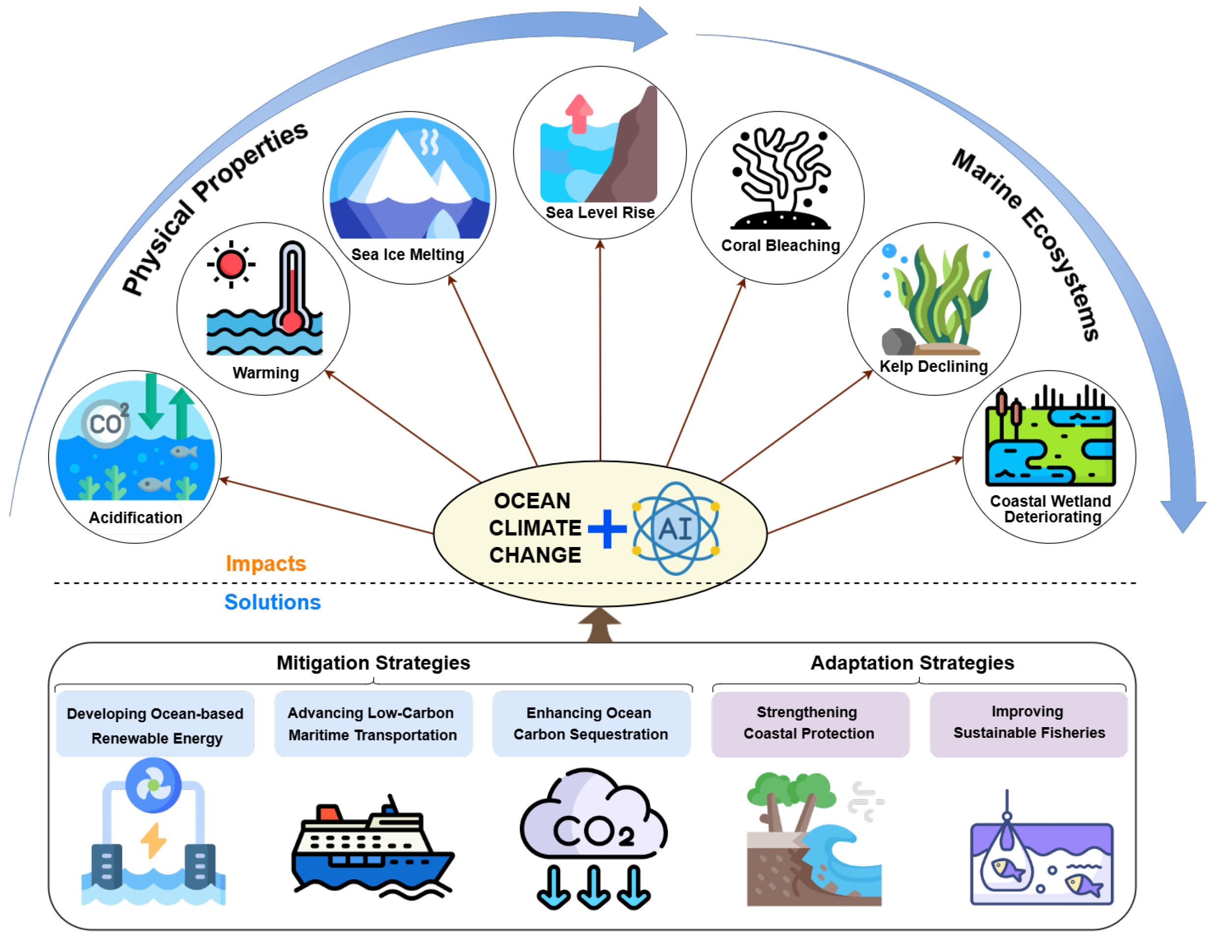
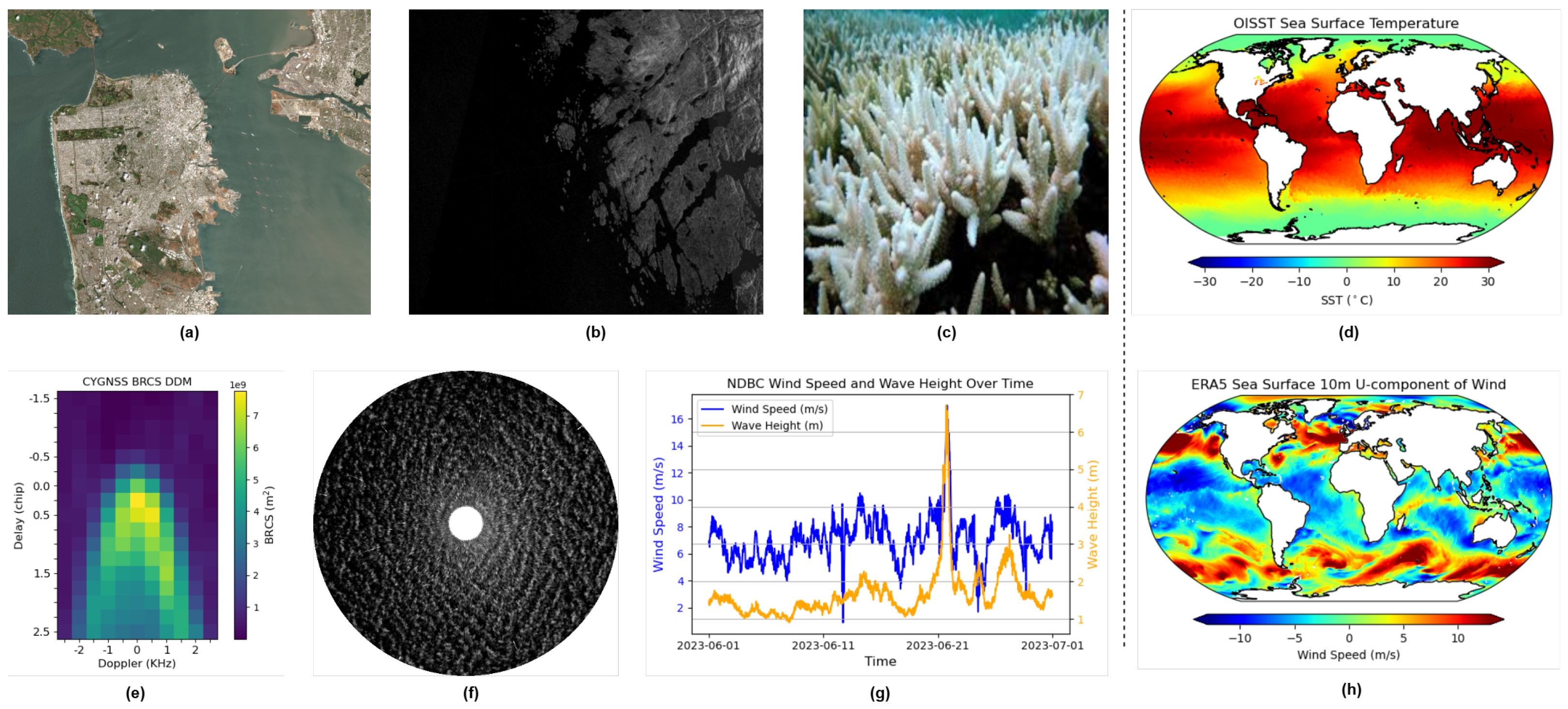
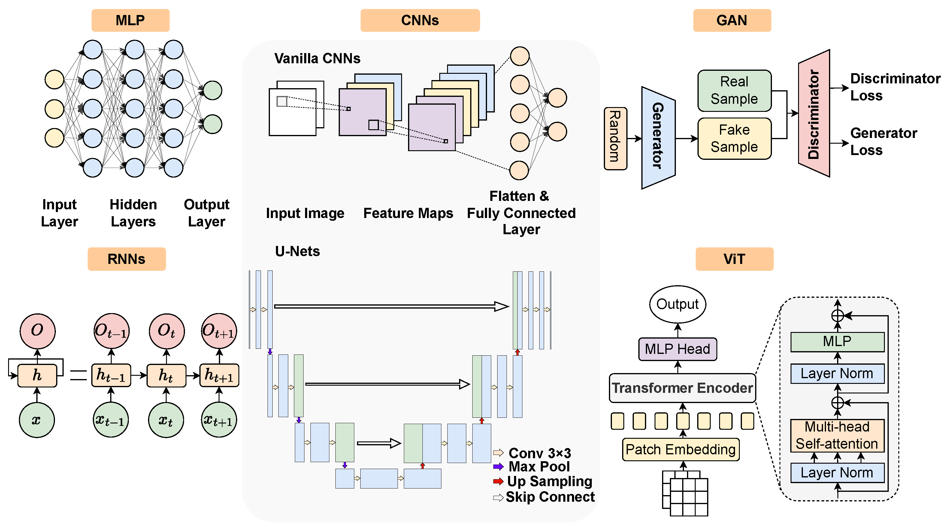
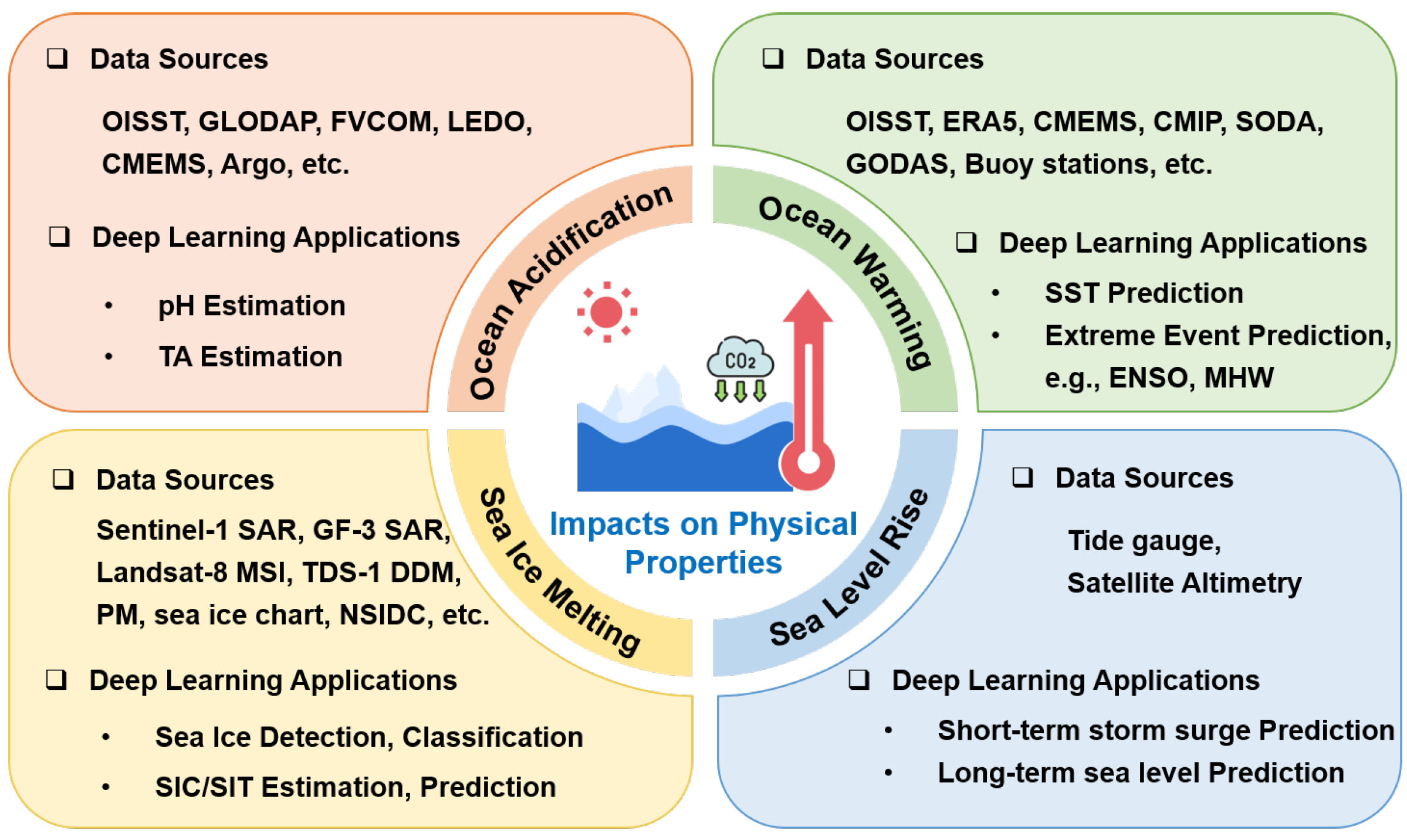
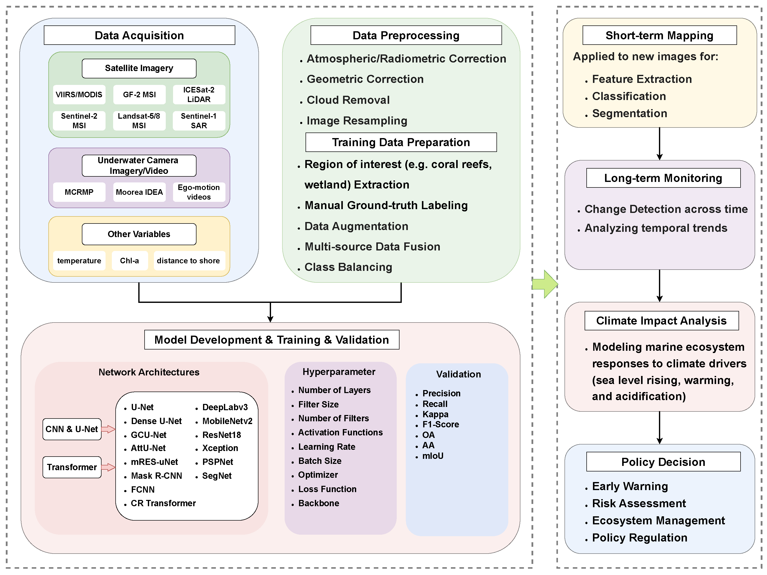
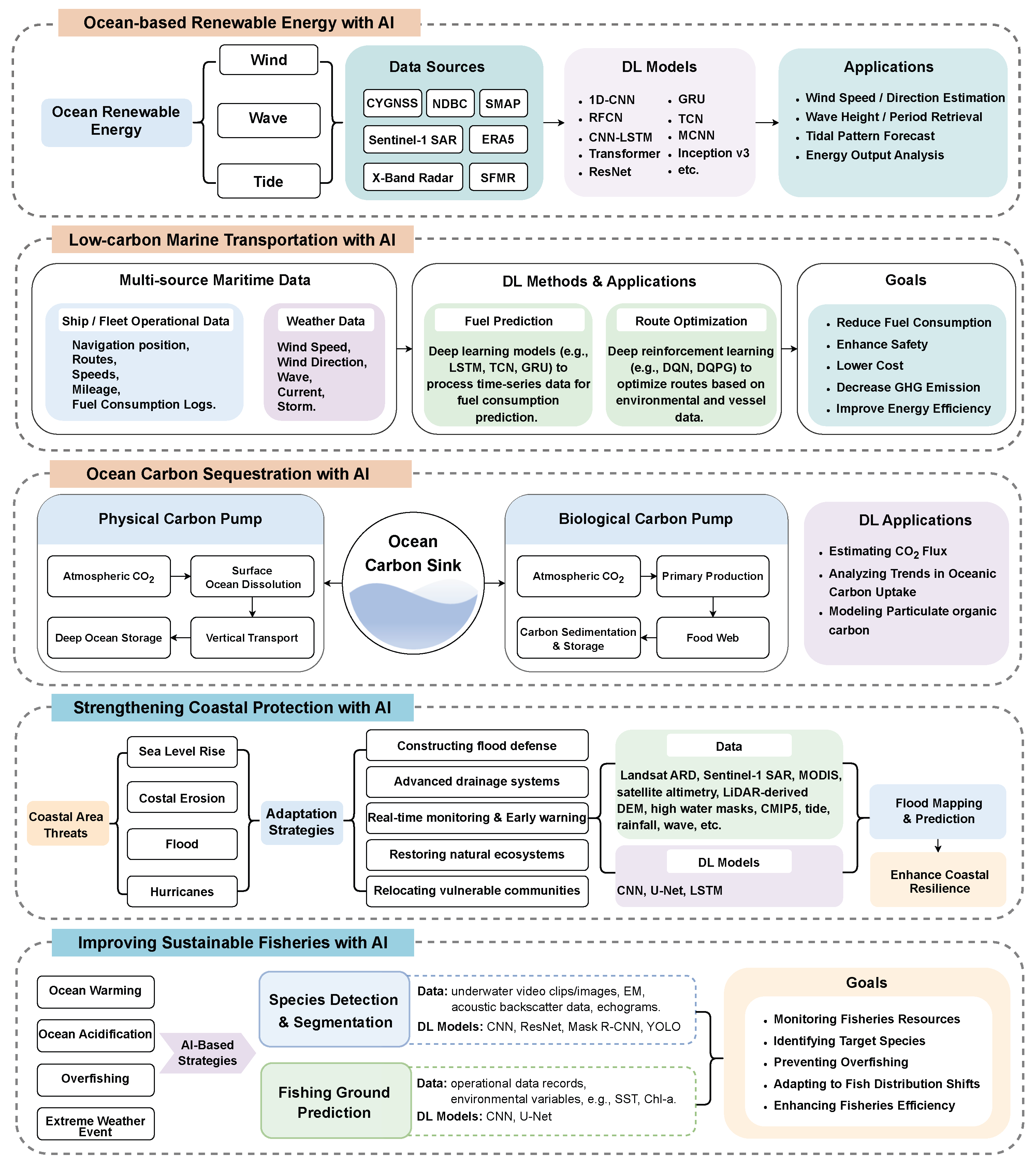
Figure 1. A brief overview of the impacts of climate change on oceans and ocean-based solutions.

Figure 2. Examples of ocean data: (a) Sentinel-2 MSI imagery; (b) Sentinel-1 SAR data; (c) Underwater coral reef photographs; (d) OISST SST data; (e) CYGNSS bistatic radar cross-section DDM data; (f) X-band radar imagery; (g) NDBC buoy observations; (h) ERA5 reanalysis data.

Figure 3. Commonly used neural network architectures in ocean studies.

Figure 4. Overview of climate change on ocean physical properties.

Figure 5. Flowchart of DL applications for monitoring climate change impacts on various marine ecosystems.

Figure 6. Different applications of AI for facilitating ocean-based climate change solutions.

Table 1. A summary of various ocean data categories.

Category	Subcategory	Widely Used Data	Source	Characteristics	Applications
Observation Data	Remote Sensing Data
	Optical	MODIS	https://modis.gsfc.nasa.gov/data/ (accessed on 1 July 2025)	36 bands from 0.4 to 1.4 µm	Temperature, chl-a, sea ice
		VIIRS	https://viirsland.gsfc.nasa.gov/ (accessed on 1 July 2025)	22 bands from 0.41 to 12.01 µm	Temperature, chl-a, sea ice
		Landsat-8 OLI/TIRS	https://landsat.gsfc.nasa.gov/satellites/landsat-8/ (accessed on 1 July 2025)	11 bands from 0.4 to 12.5 µm	Coastal wetland, e.g., mangroves
		Sentinel-2 MSI	https://browser.dataspace.copernicus.eu/ (accessed on 1 July 2025)	13 bands from 0.44 to 2.19 µm	Chl-a, coral reef
		Sentinel-3 OLCI	https://browser.dataspace.copernicus.eu/ (accessed on 1 July 2025)	21 bands from 0.4 to 1.02 µm	Chl-a, temperature
		GOCI	https://oceancolor.gsfc.nasa.gov/about/missions/goci/ (accessed on 1 July 2025)	8 bands (6 visible, 2 NIR)	Chl-a, sea ice, coastal water dynamics
		PlanetScope	https://www.planet.com/industries/education-and-research/ (accessed on 1 July 2025)	8 bands, 3–5 m per pixel	Coastal Wetland
	SAR	Sentinel-1	https://browser.dataspace.copernicus.eu/ (accessed on 1 July 2025)	C-Band	Sea ice, oil spill, ship detection
		RADARSAT-2	https://www.asc-csa.gc.ca/eng/satellites/radarsat2/ (accessed on 1 July 2025)	C-Band	Sea ice and ship detection
		RCM	https://www.asc-csa.gc.ca/eng/satellites/radarsat/ (accessed on 1 July 2025)	C-Band	Sea ice, oil spill, ship detection
		TerraSAR-X	https://earth.esa.int/eogateway/missions/terrasar-x-and-tandem-x (accessed on 1 July 2025)	X-Band	Wave, sea ice, ship detection
		ICEYE	https://www.iceye.com/sar-data (accessed on 1 July 2025)	X-Band	Flood, oil spill monitoring
	GNSS-R	TDS-1	https://merrbys.co.uk/ (accessed on 1 July 2025)	L-Band, global coverage	Sea ice, wind, wave
	GNSS-R	CYGNSS	https://cygnss.engin.umich.edu/data-products/ (accessed on 1 July 2025)	L-Band, cover 38°N and 38°S	Wind, wave, algae bloom
	Passive Microwave	AMSR-2	https://www.earthdata.nasa.gov/data/instruments/amsr2 (accessed on 1 July 2025)	Multifrequency radiometer	Temperature, sea ice concentration, and wind speed
	Lidar	ICESat-2	https://icesat-2.gsfc.nasa.gov/ (accessed on 1 July 2025)	Laser pulses at 532 nm, global coverage	Sea ice
	X-Band Radar	Furuno	https://github.com/openradar/open-radar-data (accessed on 1 July 2025)	X-Band, wavelength at 3 cm	Wind, wave, currents
	HF Radar	NOAA HF Radar National Server	https://hfradar.ndbc.noaa.gov/ (accessed on 1 July 2025)	High frequency 3–30 MHz, cover coastal areas	Surface currents, wind, wave
	Acoustic	Passive Acoustic Data	https://www.ncei.noaa.gov/products/passive-acoustic-data (accessed on 1 July 2025)	Sound waves	Fisheries
	In Situ Data
	Buoy	NDBC	https://www.ndbc.noaa.gov/ (accessed on 1 July 2025)	Mooring buoy, global distribution, real-time data	Wind, wave, air pressure
	Float	Argo	https://www.aoml.noaa.gov/argo/ (accessed on 1 July 2025)	Autonomous profiling float, global distribution	Temperature, salinity, depth
	Float	BGC-Argo	https://biogeochemical-argo.org/ (accessed on 1 July 2025)	Floats carry biological and chemical sensors	Chl-a, oxygen, nitrate, pH
	Research Vessels	GLODAP	https://glodap.info/ (accessed on 1 July 2025)	Global synthesis of ocean carbon measurements	Alkalinity, oxygen, nitrate
	Research Vessels	GO-SHIP	http://www.go-ship.org/ (accessed on 1 July 2025)	Full-depth hydrographic sections for climate monitoring	DIC, pH
	Tide Gauges	U of Hawaii Sea Level Center	https://uhslc.soest.hawaii.edu/ (accessed on 1 July 2025)	Global distribution	Sea level height, tide
	Tide Gauges	PSMSL	https://psmsl.org/ (accessed on 1 July 2025)	Global distribution	Sea level height, tide
	Underwater Images/Video	NOAA Ocean Exploration Video Portal	https://www.ncei.noaa.gov/access/ocean-exploration/video/ (accessed on 1 July 2025)	Images/videos taken by AUV or ROV	Coral reefs, undersea topography
Model Data	Physical Model	CMIP	https://pcmdi.llnl.gov/CMIP6/ (accessed on 1 July 2025)	Physical-based climate model	Temperature, precipitation, sea level, etc.
	Physical Model	WW3	https://polar.ncep.noaa.gov/waves/wavewatch/ (accessed on 1 July 2025)	Physical-based wave model	wave
	ML Model	GraphCast	https://github.com/google-deepmind/graphcast (accessed on 1 July 2025)	ML model based on GNN	Weather-related variables
Reanalysis Data	ECMWF	ERA5	https://cds.climate.copernicus.eu/datasets (accessed on 1 July 2025)	Global coverage, hourly values	Wind, wave, temperature
	U of Maryland	SODA	http://www.soda.umd.edu/ (accessed on 1 July 2025)	Global coverage	Wind, potential temperature, salinity
	NOAA	GODAS	https://psl.noaa.gov/data/gridded/data.godas.html (accessed on 1 July 2025)	Global coverage, monthly values	Temperature, oxygen, salinity
	NOAA	OISST	https://www.ncei.noaa.gov/products/optimum-interpolation-sst (accessed on 1 July 2025)	Global coverage, daily values	SST
	CMEMS	GLORYS	https://data.marine.copernicus.eu/products (accessed on 1 July 2025)	Global coverage, daily and monthly values	Temperature, salinity, currents

Disclaimer/Publisher’s Note: The statements, opinions and data contained in all publications are solely those of the individual author(s) and contributor(s) and not of MDPI and/or the editor(s). MDPI and/or the editor(s) disclaim responsibility for any injury to people or property resulting from any ideas, methods, instructions or products referred to in the content.

© 2025 by the authors. Licensee MDPI, Basel, Switzerland. This article is an open access article distributed under the terms and conditions of the Creative Commons Attribution (CC BY) license (https://creativecommons.org/licenses/by/4.0/).

Share and Cite

MDPI and ACS Style

Qiao, X.; Zhang, K.; Huang, W. Impacts of Climate Change on Oceans and Ocean-Based Solutions: A Comprehensive Review from the Deep Learning Perspective. Remote Sens. 2025, 17, 2306. https://doi.org/10.3390/rs17132306

AMA Style

Qiao X, Zhang K, Huang W. Impacts of Climate Change on Oceans and Ocean-Based Solutions: A Comprehensive Review from the Deep Learning Perspective. Remote Sensing. 2025; 17(13):2306. https://doi.org/10.3390/rs17132306

Chicago/Turabian Style

Qiao, Xin, Ke Zhang, and Weimin Huang. 2025. "Impacts of Climate Change on Oceans and Ocean-Based Solutions: A Comprehensive Review from the Deep Learning Perspective" Remote Sensing 17, no. 13: 2306. https://doi.org/10.3390/rs17132306

APA Style

Qiao, X., Zhang, K., & Huang, W. (2025). Impacts of Climate Change on Oceans and Ocean-Based Solutions: A Comprehensive Review from the Deep Learning Perspective. Remote Sensing, 17(13), 2306. https://doi.org/10.3390/rs17132306

Note that from the first issue of 2016, this journal uses article numbers instead of page numbers. See further details here.

Article Menu

Impacts of Climate Change on Oceans and Ocean-Based Solutions: A Comprehensive Review from the Deep Learning Perspective

Abstract

1. Introduction

2. Data: Foundations of Ocean Studies

2.1. Observational Data

2.1.1. Remote Sensing Data

Optical Remote Sensing

SAR

GNSS-R

Passive Microwave

LiDAR

X-Band Radar

HF Radar

Acoustic Remote Sensing

2.1.2. In Situ Observation Data

2.2. Model Data

2.3. Reanalysis Data

3. DL Models for Ocean Studies

3.1. MLP

3.2. Convolution-Based Architecture

3.2.1. Vanilla CNNs

3.2.2. U-Net

3.3. RNN

3.4. GAN

3.5. ViT

4. Impact of Climate Change on Oceans: Leveraging DL for Monitoring and Analysis

4.1. Understanding Impacts on Physical Properties via DL

4.1.1. Applying DL to Estimate Ocean pH Levels

4.1.2. DL for Predicting Ocean Warming Trends and Associated Extreme Weather Events

4.1.3. Advancing Sea Ice Monitoring and Prediction with DL

4.1.4. Predicting Sea Level Rise with DL

4.2. Unveiling Changes in Different Vulnerable Marine Ecosystems Using AI

4.2.1. DL Applications for Coral Reef Monitoring

4.2.2. Leveraging DL for Kelp Forest and Other Seaweed Ecosystems Monitoring

4.2.3. DL for Coastal Wetland Mapping and Analysis

5. Ocean-Based Climate Change Solutions Enhanced by DL

5.1. Mitigation Strategies Using DL

5.1.1. Developing Ocean-Based Renewable Energy with DL

5.1.2. Advancing Low-Carbon Maritime Transportation Through AI

5.1.3. DL Applications in Ocean Carbon Sink

5.2. Adaptation Strategies Supported by DL

5.2.1. Strengthening Coastal Protection with DL

5.2.2. Improving Fisheries Management Leveraging DL

6. Conclusions and Future Perspectives

6.1. Summary

6.2. Challenges

6.2.1. Interpolation-Induced Errors

6.2.2. Insufficient Spatiotemporal Validation

6.2.3. Lack of Uncertainty Quantification

6.2.4. Limited Explainability

6.2.5. Poorly Modeled Ocean Processes

6.3. Directions for Future Research

6.3.1. Reducing Interpolation-Induced Errors

6.3.2. Enhancing Validation Across Space and Time

6.3.3. Quantifying Model Uncertainty

6.3.4. Advancing Explainability

6.3.5. Towards Physic-Informed Neural Networks (PINNs)

Author Contributions

Funding

Data Availability Statement

Acknowledgments

Conflicts of Interest

References

Share and Cite

Article Metrics

Article Access Statistics

Further Information

Guidelines

MDPI Initiatives

Follow MDPI