
Few-Shot Unsupervised Domain Adaptation Based on Refined Bi-Directional Prototypical Contrastive Learning for Cross-Scene Hyperspectral Image Classification

 and
and
Abstract

1. Introduction
- 1.
- We propose a refined bi-directional prototypical contrastive learning (RBPCL) framework for the few-shot unsupervised domain adaptation (FUDA) setting in hyperspectral cross-scene classification (HSICC) tasks. So far as we know, this work is the first attempt to tackle the FUDA setting in the field of hyperspectral cross-scene classification.
- 2.
- We leverage refined in-domain and bi-directional cross-domain prototypical contrastive learning to simultaneously realize efficient category-discriminative feature representation and cross-domain alignment in an end-to-end, unsupervised, and adaptive pattern.
- 3.
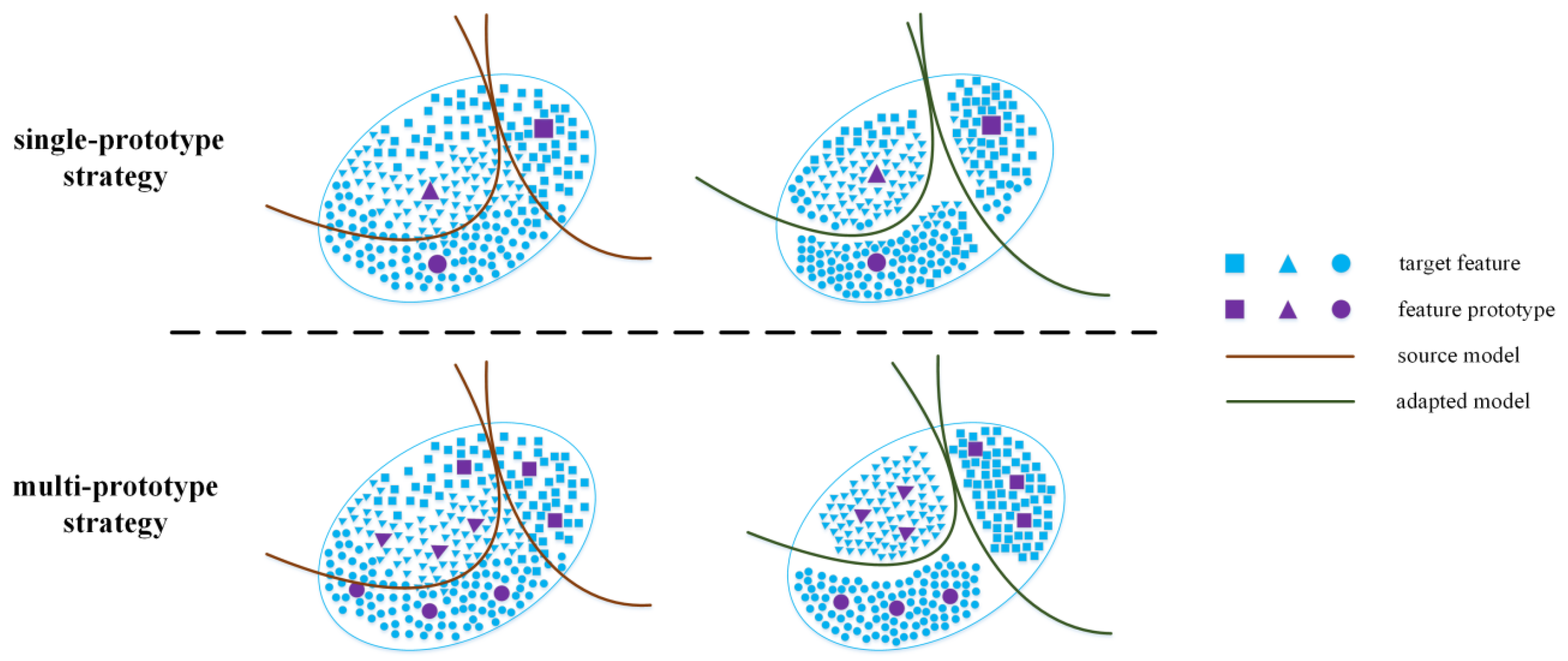
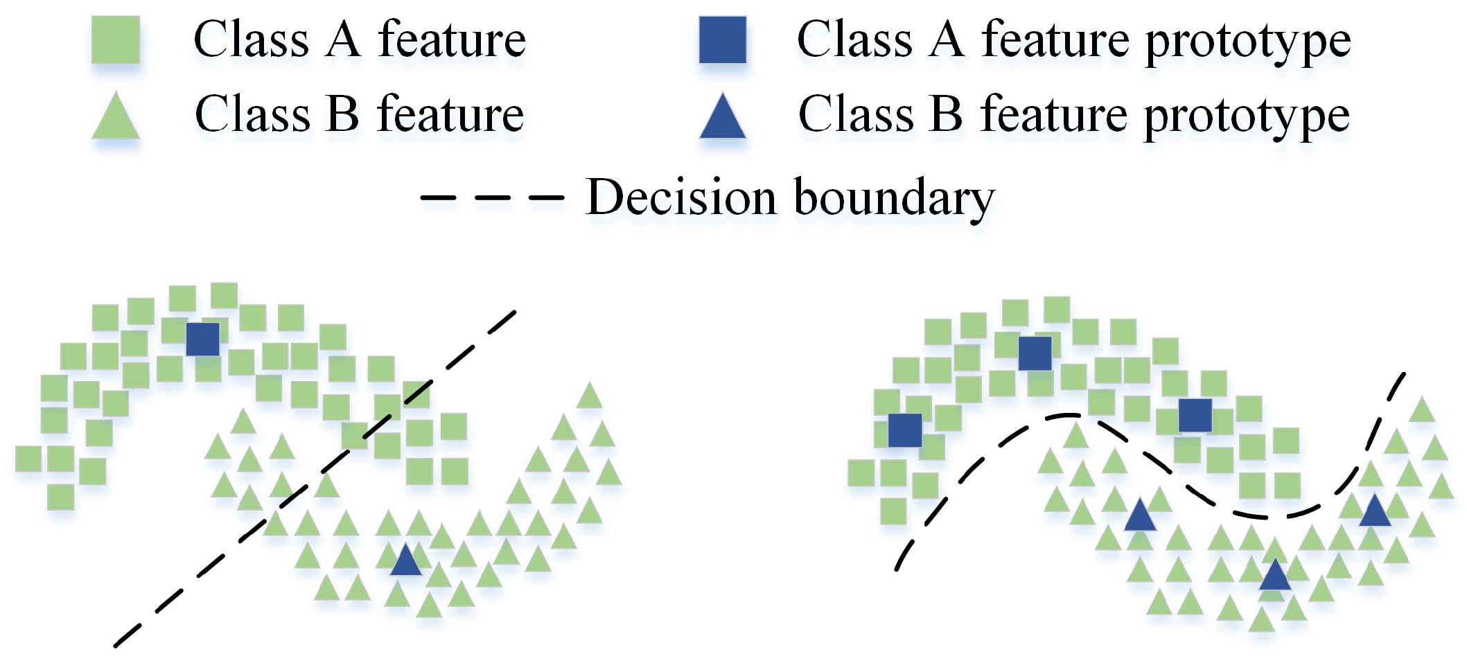
- We employ the class-balanced multicentric dynamic (BMD) prototype strategy to facilitate the generation of more representative and robust clustering prototypes. Furthermore, we design a Siamese-style distance metric loss function to gather intra-class features while segregating inter-class features, ultimately promoting refined prototypical self-supervised learning.
- 4.
- We carry out exhaustive crossover experiments on five data pairs with different degrees of domain shifts, including hyperspectral images of spatially disjoint geographical regions and multitemporal images, to demonstrate the effectiveness of the proposed method. It is noteworthy that the practical value of our RBPCL is demonstrated using three ultralow-altitude hyperspectral images, independently collected by an unmanned aerial vehicle (UAV) under varying geographic locations and illumination conditions.
2. Related Work
2.1. Unsupervised Domain Adaptation
2.2. Prototypical Contrastive Learning
2.3. Few-Shot Unsupervised Domain Adaptation
3. Methodology
3.1. Problem Definition
3.2. Overall Framework
3.3. In-Domain Refined Prototypical Contrastive Learning
3.4. Bi-Directional Cross-Domain Prototypical Contrastive Learning
3.5. Adaptive Prototypical Classifier Learning
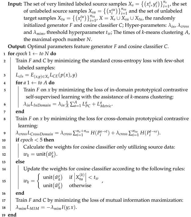
| Algorithm 1: Training Procedure for RBPCL |
 |
4. Experiments
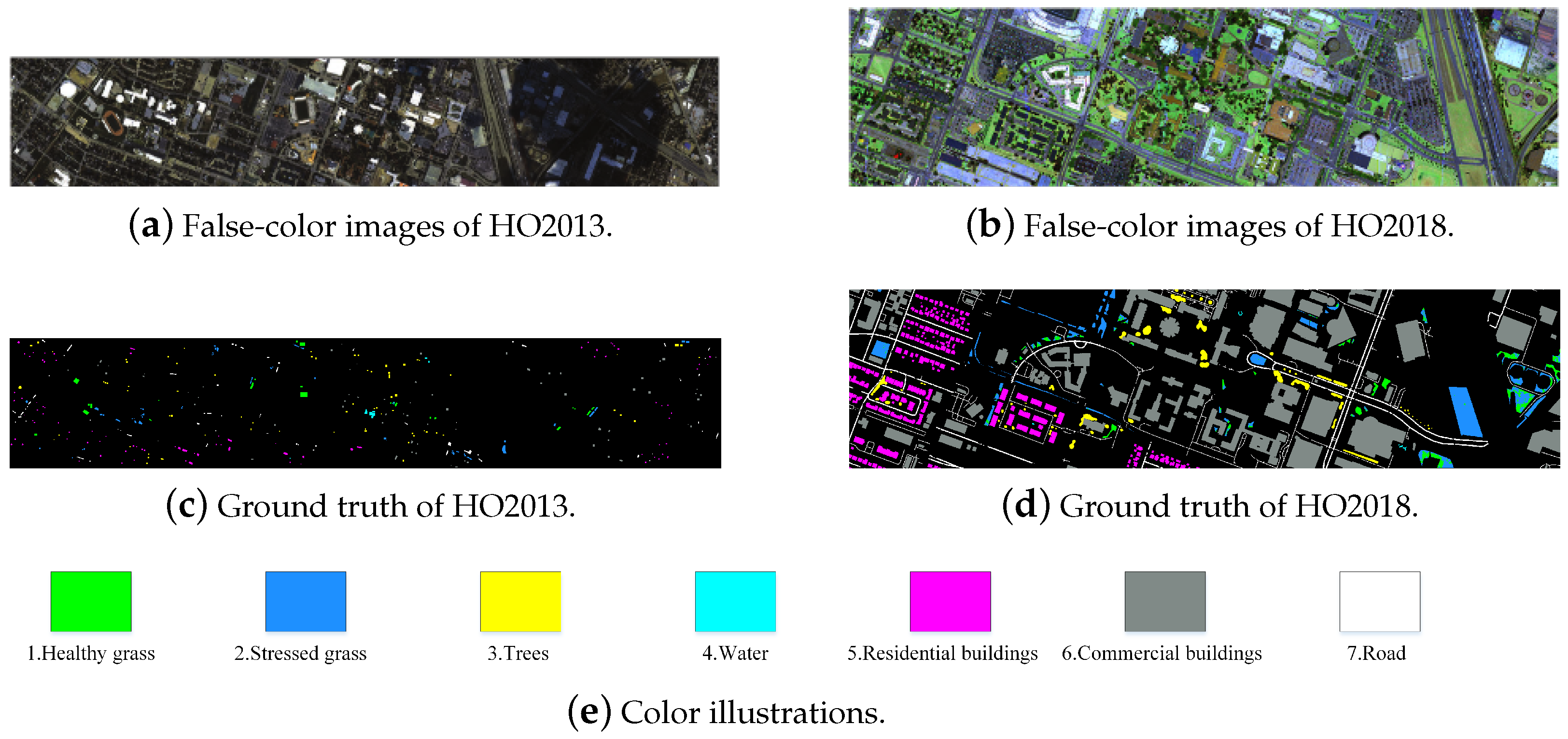
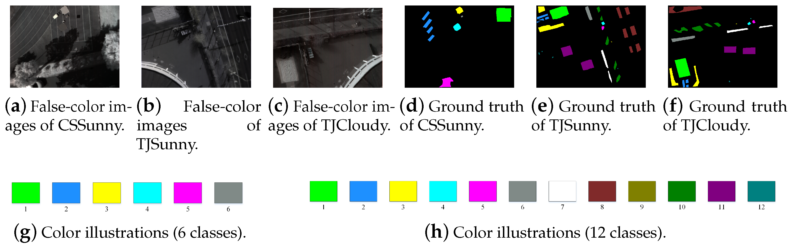
4.1. Datasets
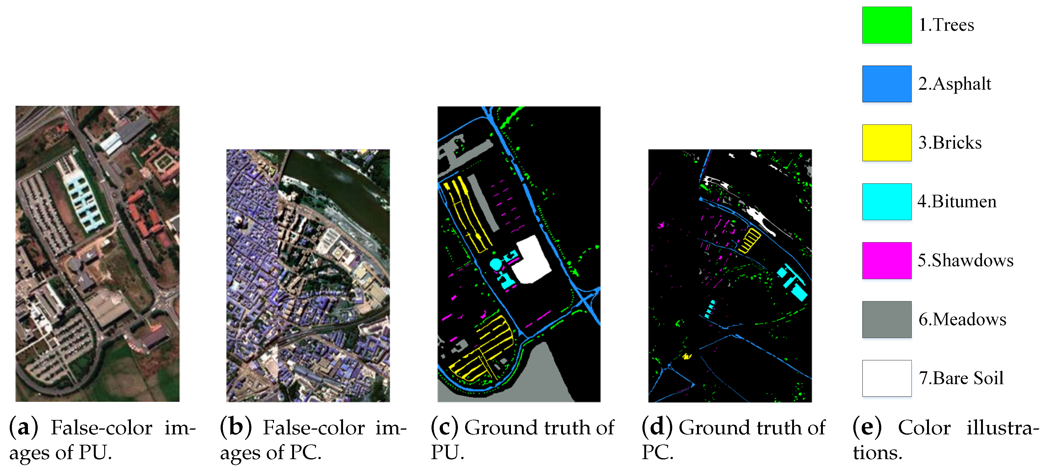
4.1.1. Pavia Data Pair
4.1.2. Houston Data Pair
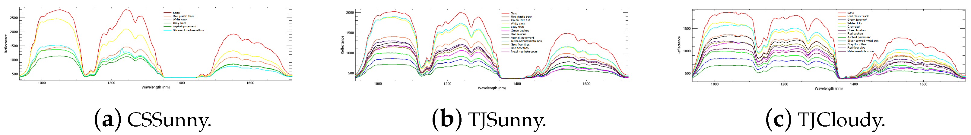
4.1.3. Self-Collected Data Pairs
4.2. Implementation Details
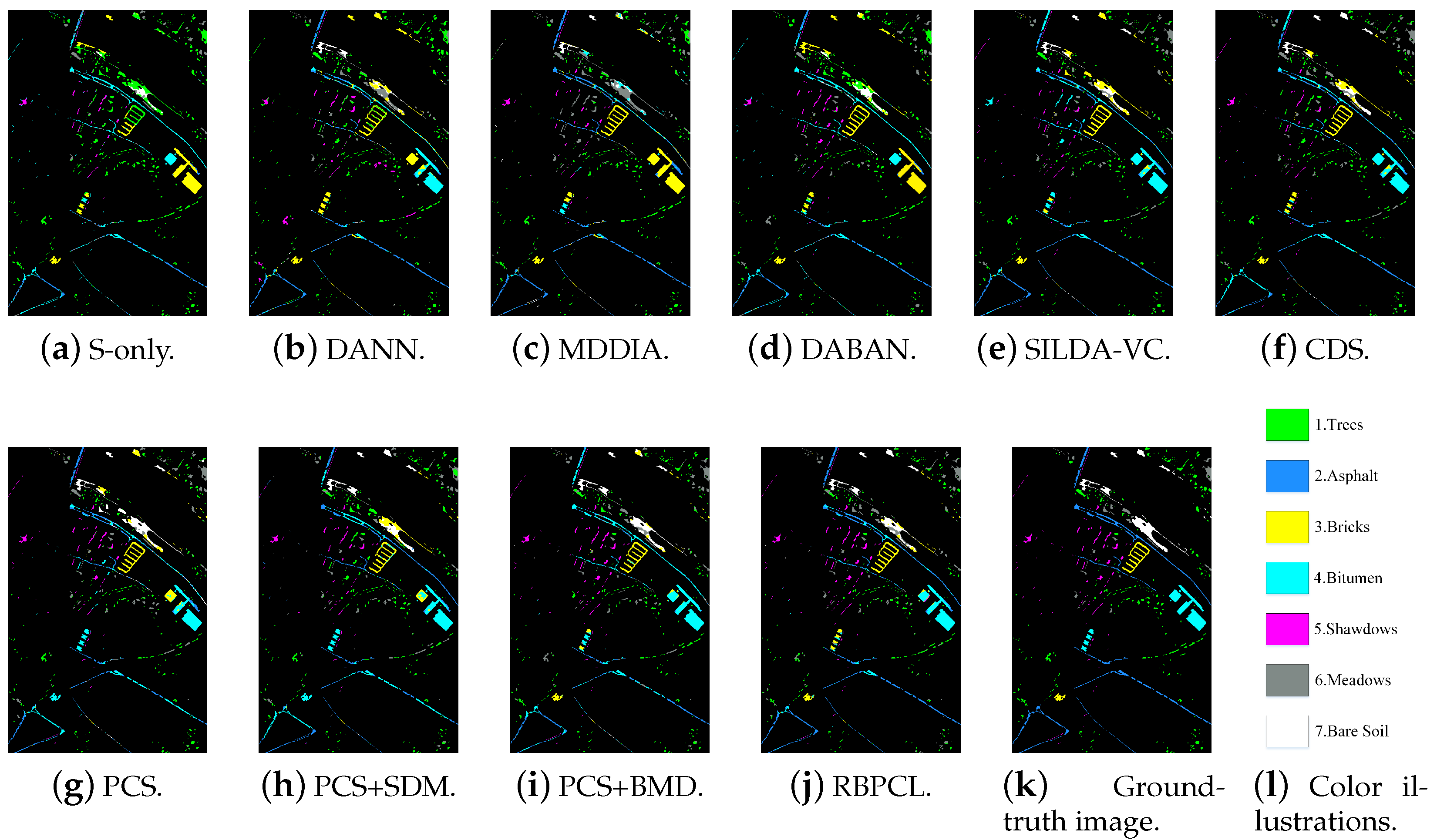
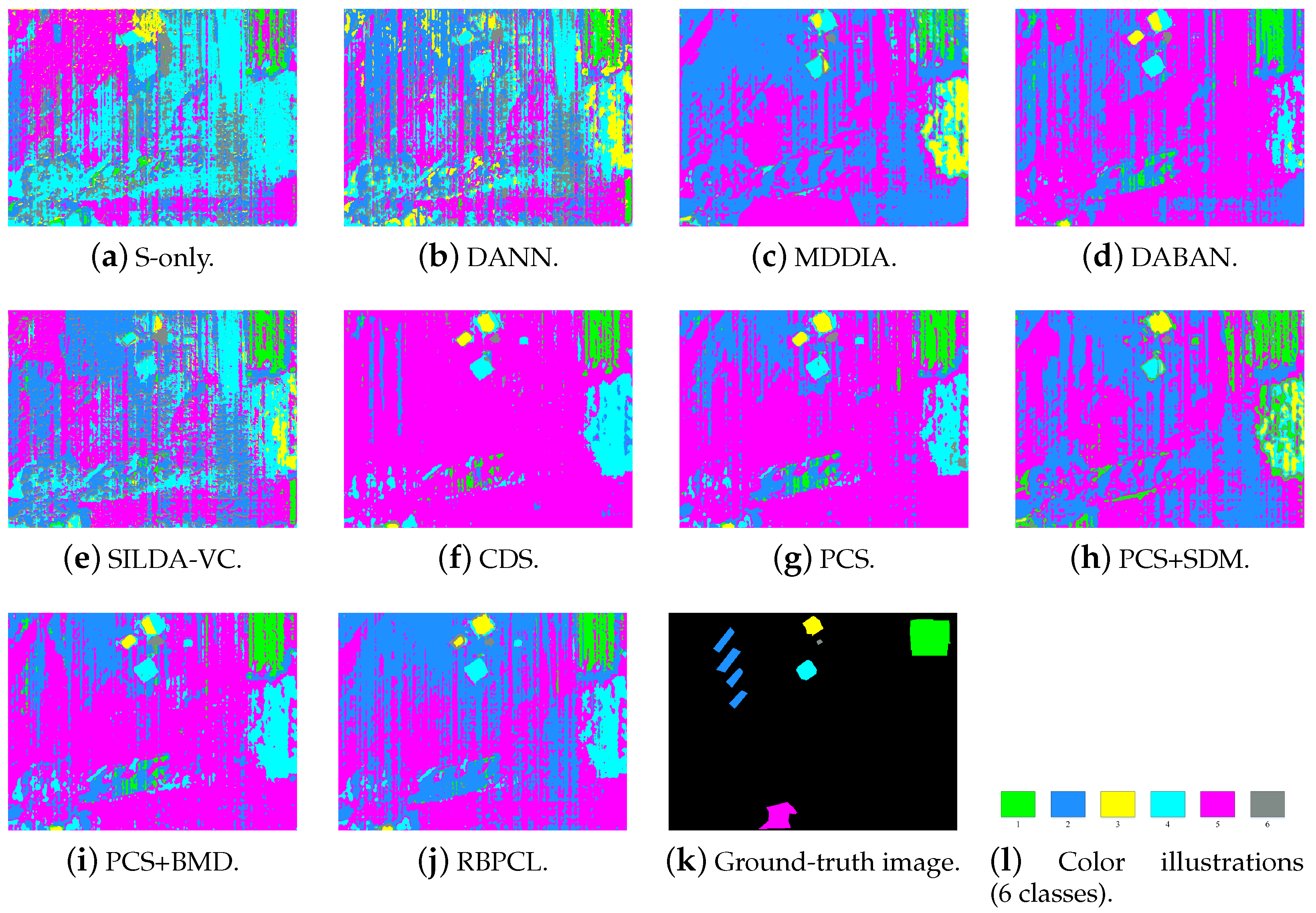
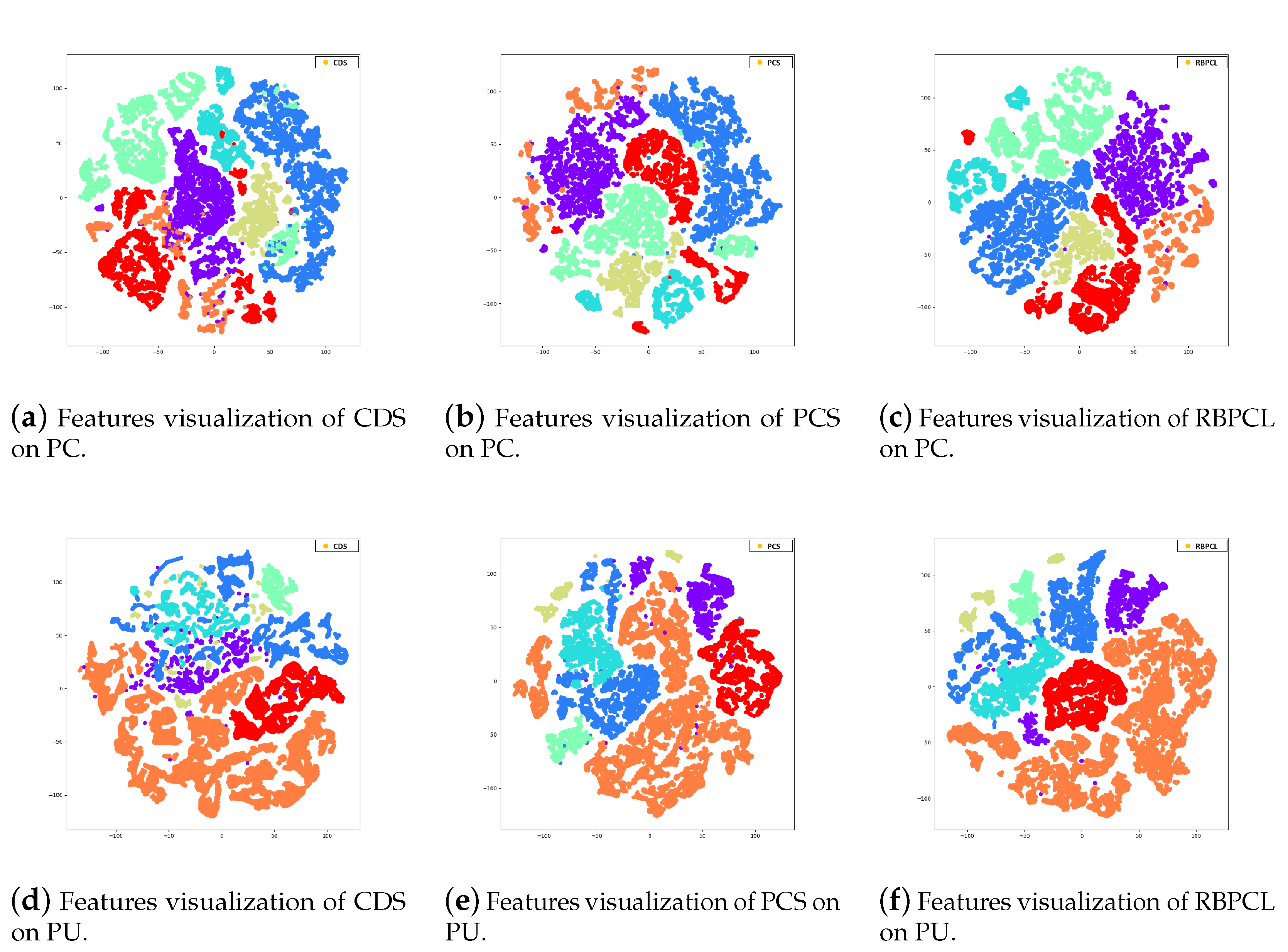
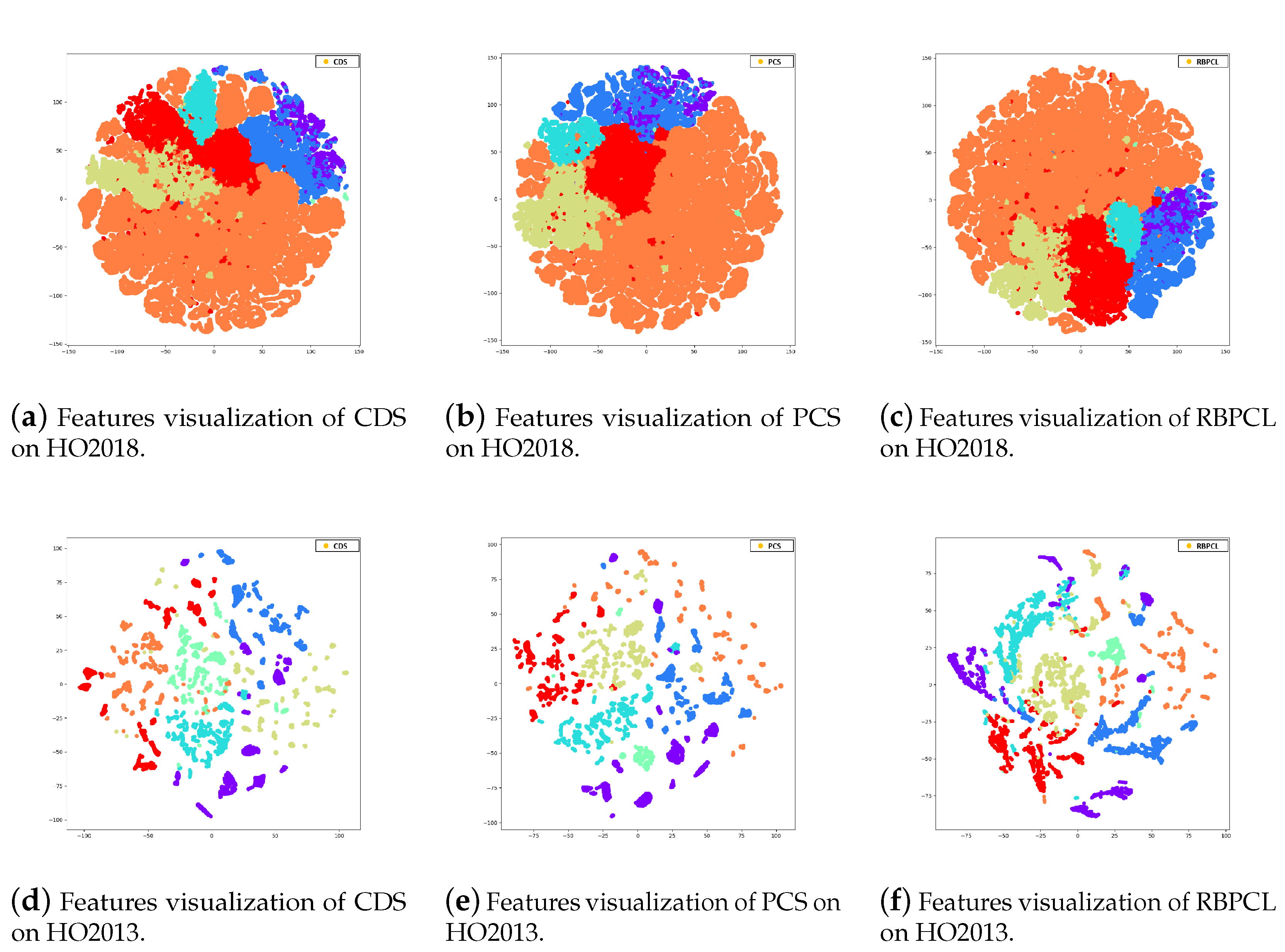
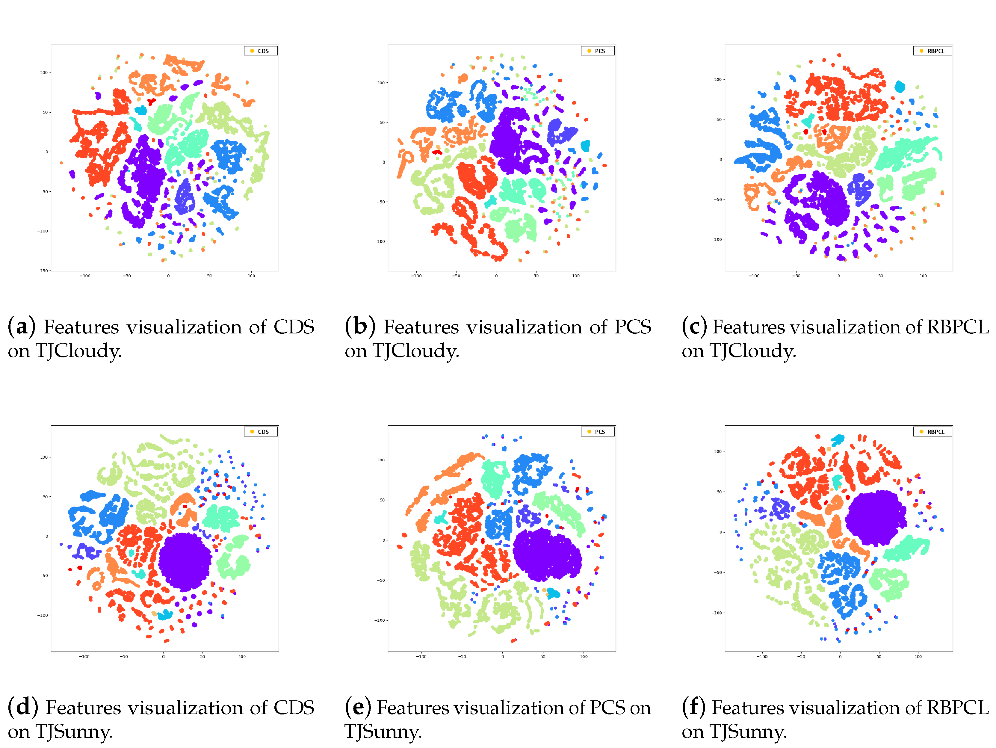
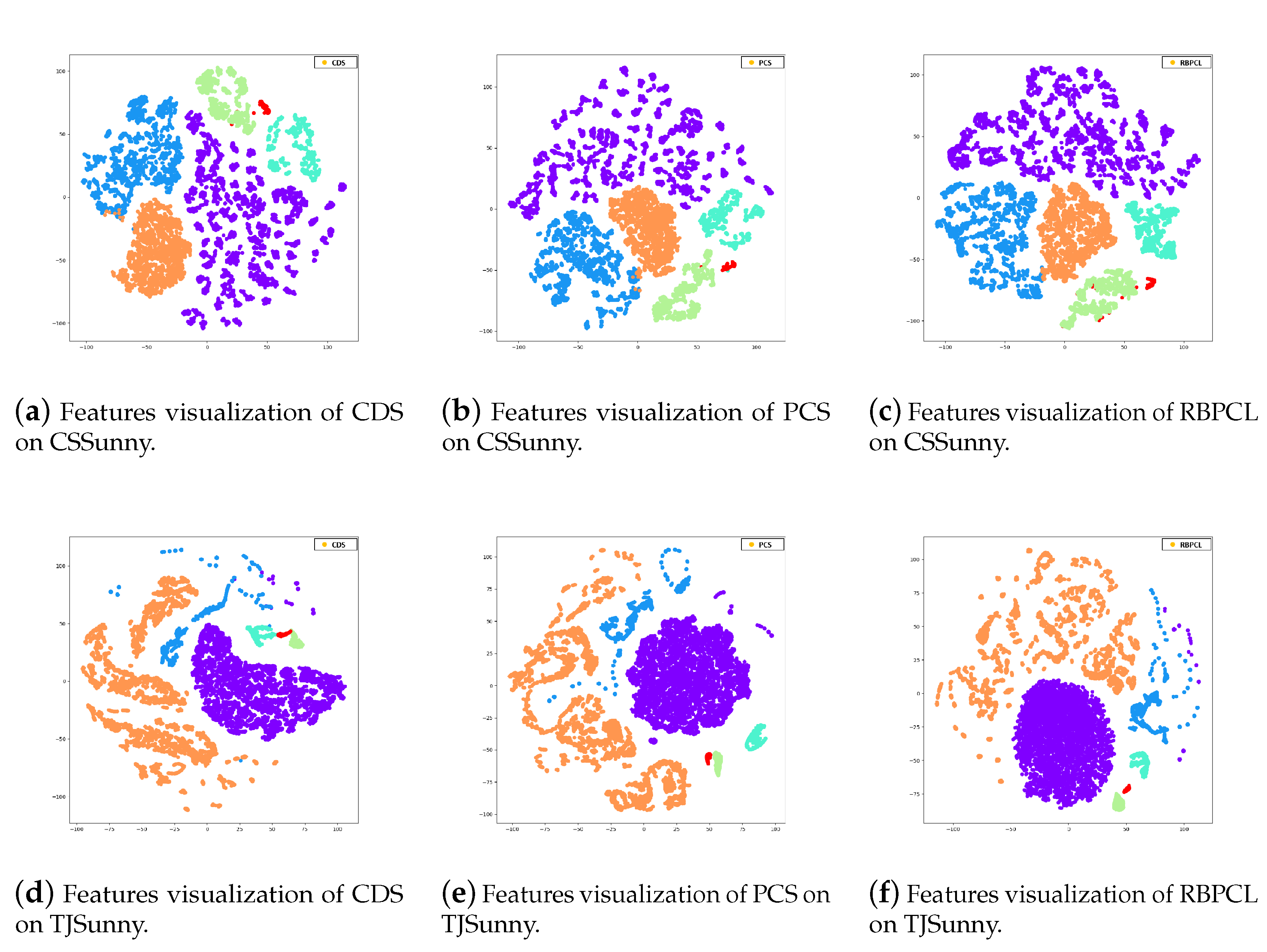
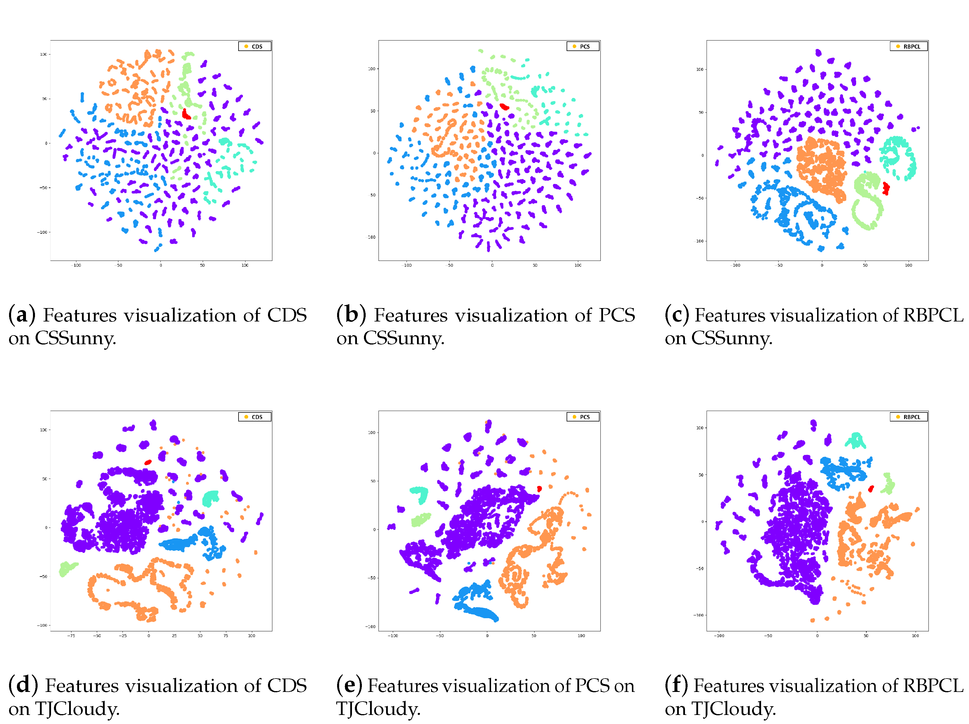
4.3. Results and Ablation Analysis
4.4. Impact of Different Parameter Settings
4.5. Effects of Losses
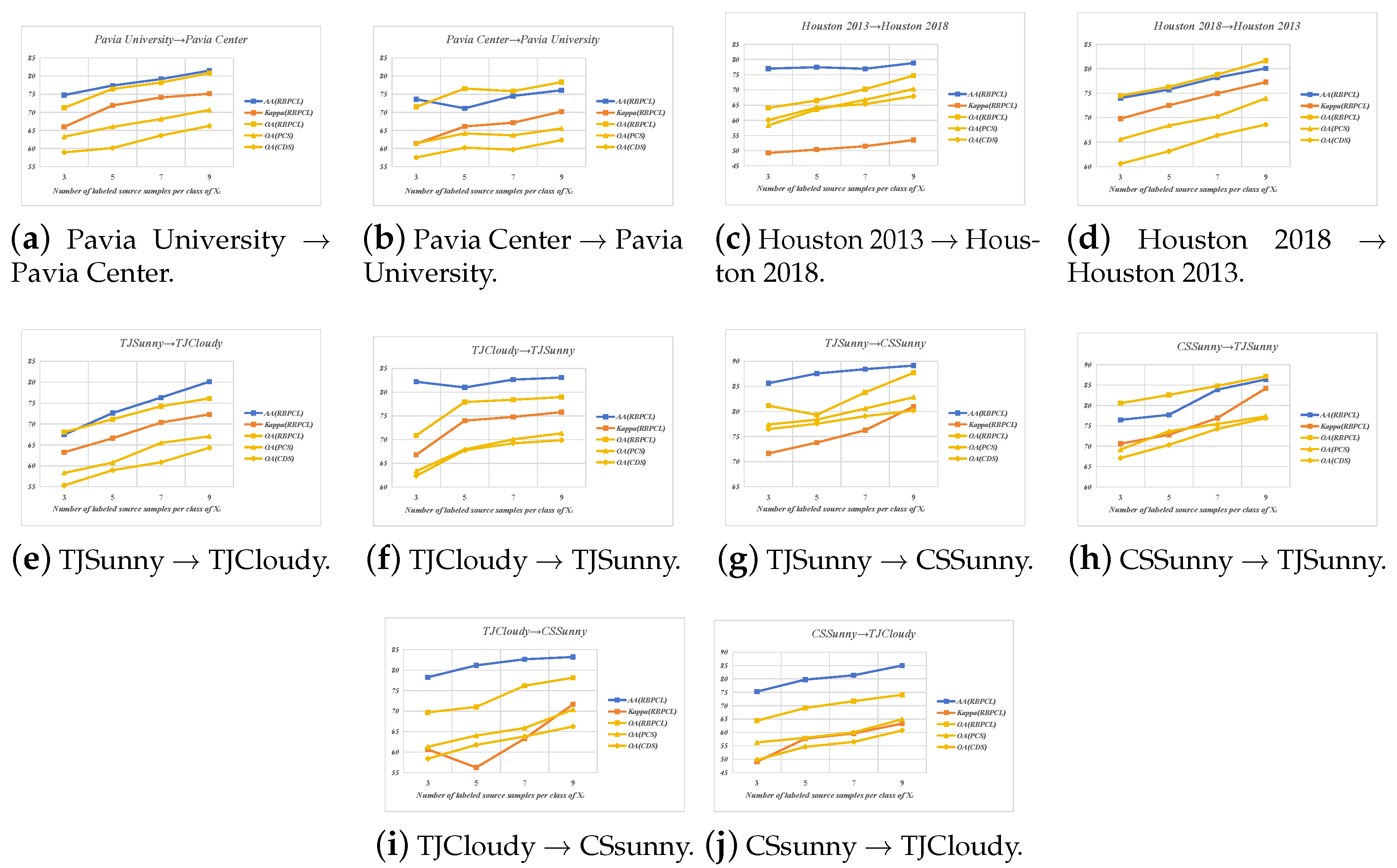
4.6. Impact of the Labeled Samples in Source Domain

| AA | OA | Kappa | |||
|---|---|---|---|---|---|
| 1 | 1 | 0.05 | 72.39 | 72.01 | 63.74 |
| 0.5 | 1 | 0.05 | 71.3 | 68.65 | 62.59 |
| 1 | 0.5 | 0.05 | 74.57 | 71.24 | 65.96 |
| 0.5 | 0.5 | 0.05 | 69.93 | 69.22 | 61.81 |
| 1 | 1 | 0.01 | 72.61 | 70.25 | 64.15 |
| 0.5 | 1 | 0.01 | 70.84 | 68.38 | 62.07 |
| 1 | 0.5 | 0.01 | 73.45 | 70.69 | 64.28 |
| 0.5 | 0.5 | 0.01 | 68.73 | 69.47 | 61.46 |
| AA | OA | Kappa | |||
|---|---|---|---|---|---|
| 1 | 1 | 0.05 | 72.47 | 70.69 | 60.24 |
| 0.5 | 1 | 0.05 | 71.22 | 69.38 | 59.77 |
| 1 | 0.5 | 0.05 | 73.6 | 71.48 | 61.35 |
| 0.5 | 0.5 | 0.05 | 70.86 | 68.56 | 59.14 |
| 1 | 1 | 0.01 | 71.67 | 70.84 | 59.58 |
| 0.5 | 1 | 0.01 | 70.75 | 67.92 | 58.76 |
| 1 | 0.5 | 0.01 | 72.51 | 68.89 | 60.43 |
| 0.5 | 0.5 | 0.01 | 70.83 | 67.15 | 59.06 |
| AA | OA | Kappa | |||
|---|---|---|---|---|---|
| 1 | 1 | 0.05 | 81.77 | 80.04 | 69.81 |
| 0.5 | 1 | 0.05 | 80.13 | 78.66 | 70.28 |
| 1 | 0.5 | 0.05 | 85.62 | 81.15 | 71.64 |
| 0.5 | 0.5 | 0.05 | 79.78 | 77.59 | 70.94 |
| 1 | 1 | 0.01 | 80.37 | 79.41 | 69.36 |
| 0.5 | 1 | 0.01 | 80.21 | 77.64 | 69.13 |
| 1 | 0.5 | 0.01 | 82.31 | 81.86 | 70.02 |
| 0.5 | 0.5 | 0.01 | 79.55 | 76.97 | 68.87 |
| AA | OA | Kappa | |||
|---|---|---|---|---|---|
| 1 | 1 | 0.05 | 72.61 | 76.33 | 65.24 |
| 0.5 | 1 | 0.05 | 71.06 | 76.87 | 66.42 |
| 1 | 0.5 | 0.05 | 76.47 | 80.55 | 70.62 |
| 0.5 | 0.5 | 0.05 | 72.18 | 77.35 | 67.53 |
| 1 | 1 | 0.01 | 71.36 | 75.47 | 64.95 |
| 0.5 | 1 | 0.01 | 70.11 | 76.04 | 65.88 |
| 1 | 0.5 | 0.01 | 74.39 | 78.76 | 68.13 |
| 0.5 | 0.5 | 0.01 | 70.99 | 74.82 | 66.75 |
| Method | PU → PC | HO2013 → HO2018 | TJSunny → TJCloudy | TJSunny → CSSunny | TJCloudy → CSSunny |
|---|---|---|---|---|---|
| 49.79/48.97/39.15 | 47.40/37.10/18.75 | 44.38/39.08/32.29 | 67.81/58.06/42.26 | 49.07/47.05/35.53 | |
| 56.74/52.11/43.98 | 56.22/41.53/24.87 | 51.63/49.16/43.21 | 72.10/63.88/51.42 | 62.52/53.31/44.48 | |
| 64.37/60.09/52.34 | 65.56/57.93/42.75 | 60.74/57.37/52.46 | 77.34/75.73/62.19 | 70.49/62.16/51.83 | |
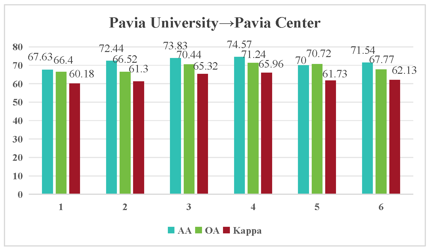
| 74.57/71.24/65.96 | 77.01/64.09/49.27 | 67.45/68.05/63.23 | 85.62/81.15/71.64 | 78.26/69.69/60.65 |
| Method | PC → PU | HO2018 → HO2013 | TJCloudy → TJSunny | CSSunny → TJSunny | CSSunny → TJCloudy |
|---|---|---|---|---|---|
| 55.51/40.68/30.96 | 39.05/42.36/32.22 | 50.46/50.25/44.32 | 62.59/41.55/28.28 | 52.67/28.18/15.94 | |
| 60.50/49.37/39.61 | 52.08/50.62/41.97 | 62.72/54.52/48.44 | 68.97/60.65/41.03 | 60.46/40.73/30.51 | |
| 65.93/58.82/50.06 | 63.63/61.79/54.45 | 71.83/66.39/61.81 | 72.36/70.24/57.89 | 67.28/55.19/38.72 | |
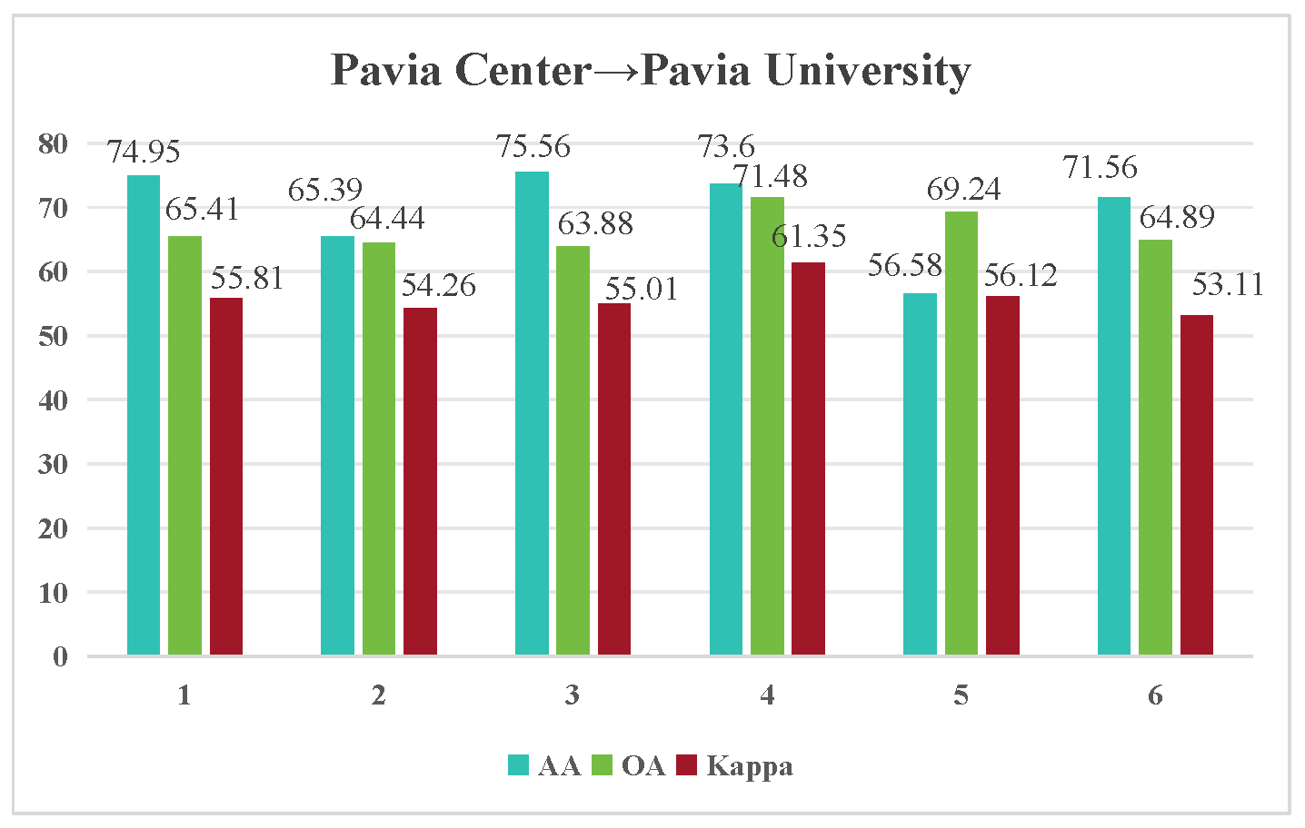
| 73.60/71.48/61.35 | 74.00/74.48/69.79 | 82.18/70.88/66.78 | 76.47/80.55/70.62 | 75.25/64.38/49.04 |
5. Discussion
6. Conclusions
Author Contributions
Funding
Data Availability Statement
Conflicts of Interest
References
- Camps-Valls, G.; Tuia, D.; Bruzzone, L.; Benediktsson, J.A. Advances in Hyperspectral Image Classification: Earth Monitoring with Statistical Learning Methods. IEEE Signal Process. Mag. 2014, 31, 45–54. [Google Scholar] [CrossRef]
- Ghamisi, P.; Yokoya, N.; Li, J.; Liao, W.; Liu, S.; Plaza, J.; Rasti, B.; Plaza, A. Advances in Hyperspectral Image and Signal Processing: A Comprehensive Overview of the State of the Art. IEEE Geosci. Remote. Sens. Mag. 2017, 5, 37–78. [Google Scholar] [CrossRef]
- He, L.; Li, J.; Liu, C.; Li, S. Recent Advances on Spectral–Spatial Hyperspectral Image Classification: An Overview and New Guidelines. IEEE Trans. Geosci. Remote Sens. 2018, 56, 1579–1597. [Google Scholar] [CrossRef]
- Kumar, B.; Dikshit, O.; Gupta, A.; Singh, M.K. Feature extraction for hyperspectral image classification: A review. Int. J. Remote Sens. 2020, 41, 6248–6287. [Google Scholar] [CrossRef]
- Samaniego, L.; Bárdossy, A.; Schulz, K. Supervised Classification of Remotely Sensed Imagery Using a Modified k-NN Technique. IEEE Trans. Geosci. Remote Sens. 2008, 46, 2112–2125. [Google Scholar] [CrossRef]
- Chang, C.I. Statistical Detection Theory Approach to Hyperspectral Image Classification. IEEE Trans. Geosci. Remote Sens. 2019, 57, 2057–2074. [Google Scholar] [CrossRef]
- Imani, M.; Ghassemian, H. An overview on spectral and spatial information fusion for hyperspectral image classification: Current trends and challenges. Inf. Fusion 2020, 59, 59–83. [Google Scholar] [CrossRef]
- Wan, Y.; Fan, Y.; Jin, M. Application of hyperspectral remote sensing for supplementary investigation of polymetallic deposits in Huaniushan ore region, northwestern China. Sci. Rep. 2021, 11, 440. [Google Scholar] [CrossRef]
- Meng, S.; Wang, X.; Hu, X.; Luo, C.; Zhong, Y. Deep learning-based crop mapping in the cloudy season using one-shot hyperspectral satellite imagery. Comput. Electron. Agric. 2021, 186, 106188. [Google Scholar] [CrossRef]
- Zhang, F.; Li, X.; Qiu, S.; Feng, J.; Wang, D.; Wu, X.; Cheng, Q. Hyperspectral imaging combined with convolutional neural network for outdoor detection of potato diseases. In Proceedings of the 2021 6th International Symposium on Computer and Information Processing Technology (ISCIPT), Changsha, China, 11–13 June 2021; pp. 846–850. [Google Scholar]
- Li, S.; Song, W.; Fang, L.; Chen, Y.; Ghamisi, P.; Benediktsson, J.A. Deep Learning for Hyperspectral Image Classification: An Overview. IEEE Trans. Geosci. Remote Sens. 2019, 57, 6690–6709. [Google Scholar] [CrossRef]
- Paoletti, M.E.; Haut, J.M.; Plaza, J.; Plaza, A.J. Deep learning classifiers for hyperspectral imaging: A review. ISPRS J. Photogramm. Remote Sens. 2019, 158, 279–317. [Google Scholar] [CrossRef]
- Liu, B.; Yu, A.; Yu, X.; Wang, R.; Gao, K.; Guo, W. Deep Multiview Learning for Hyperspectral Image Classification. IEEE Trans. Geosci. Remote Sens. 2021, 59, 7758–7772. [Google Scholar] [CrossRef]
- Liu, Q.; Xiao, L.; Yang, J.; Chan, J.C.W. Content-Guided Convolutional Neural Network for Hyperspectral Image Classification. IEEE Trans. Geosci. Remote Sens. 2020, 58, 6124–6137. [Google Scholar] [CrossRef]
- Wang, H.; Cheng, Y.; Chen, C.L.P.; Wang, X. Broad Graph Convolutional Neural Network and Its Application in Hyperspectral Image Classification. IEEE Trans. Emerg. Top. Com. Intell. 2023, 7, 610–616. [Google Scholar] [CrossRef]
- Yu, C.; Gong, B.; Song, M.; Zhao, E.; Chang, C.I. Multiview Calibrated Prototype Learning for Few-Shot Hyperspectral Image Classification. IEEE Trans. Geosci. Remote Sens. 2022, 60, 5544713. [Google Scholar] [CrossRef]
- Deng, C.; Xue, Y.; Liu, X.; Li, C.; Tao, D. Active Transfer Learning Network: A Unified Deep Joint Spectral–Spatial Feature Learning Model for Hyperspectral Image Classification. IEEE Trans. Geosci. Remote Sens. 2019, 57, 1741–1754. [Google Scholar] [CrossRef]
- Su, Y.; Gao, L.; Jiang, M.; Plaza, A.J.; Sun, X.; Zhang, B. NSCKL: Normalized Spectral Clustering With Kernel-Based Learning for Semisupervised Hyperspectral Image Classification. IEEE Trans. Cybern. 2022, 53, 6649–6662. [Google Scholar] [CrossRef]
- Su, Y.; Chen, J.; Gao, L.; Plaza, A.J.; Jiang, M.; Xu, X.; Sun, X.; Li, P. ACGT-Net: Adaptive Cuckoo Refinement-Based Graph Transfer Network for Hyperspectral Image Classification. IEEE Trans. Geosci. Remote Sens. 2023, 61, 5521314. [Google Scholar] [CrossRef]
- Liu, H.; Li, W.; Xia, X.G.; Zhang, M.; Gao, C.; Tao, R. Spectral Shift Mitigation for Cross-Scene Hyperspectral Imagery Classification. IEEE J. Sel. Topics Appl. Earth Observ. Remote Sens. 2021, 14, 6624–6638. [Google Scholar] [CrossRef]
- Peng, J.; Huang, Y.; Sun, W.; Chen, N.; Ning, Y.; Du, Q. Domain Adaptation in Remote Sensing Image Classification: A Survey. IEEE J. Sel. Topics Appl. Earth Observ. Remote Sens. 2022, 15, 9842–9859. [Google Scholar] [CrossRef]
- Pan, S.J.; Yang, Q. A Survey on Transfer Learning. IEEE Trans. Knowl. Data Eng. 2010, 22, 1345–1359. [Google Scholar] [CrossRef]
- Zhang, Y.; Li, W.; Tao, R.; Peng, J.; Du, Q.; Cai, Z. Cross-Scene Hyperspectral Image Classification With Discriminative Cooperative Alignment. IEEE Trans. Geosci. Remote Sens. 2021, 59, 9646–9660. [Google Scholar] [CrossRef]
- Liu, T.; Zhang, X.; Gu, Y. Unsupervised Cross-Temporal Classification of Hyperspectral Images With Multiple Geodesic Flow Kernel Learning. IEEE Trans. Geosci. Remote Sens. 2019, 57, 9688–9701. [Google Scholar] [CrossRef]
- Wang, H.; Cheng, Y.; Chen, C.L.P.; Wang, X. Hyperspectral Image Classification Based on Domain Adversarial Broad Adaptation Network. IEEE Trans. Geosci. Remote Sens. 2022, 60, 5517813. [Google Scholar] [CrossRef]
- Cheng, Y.; Chen, Y.; Kong, Y.; Wang, X. Soft Instance-Level Domain Adaptation With Virtual Classifier for Unsupervised Hyperspectral Image Classification. IEEE Trans. Geosci. Remote Sens. 2023, 61, 5509013. [Google Scholar] [CrossRef]
- Persello, C.; Bruzzone, L. Kernel-Based Domain-Invariant Feature Selection in Hyperspectral Images for Transfer Learning. IEEE Trans. Geosci. Remote Sens. 2016, 54, 2615–2626. [Google Scholar] [CrossRef]
- Yu, C.; Liu, C.; Yu, H.; Song, M.; Chang, C.I. Unsupervised Domain Adaptation With Dense-Based Compaction for Hyperspectral Imagery. IEEE J. Sel. Topics Appl. Earth Observ. Remote Sens. 2021, 14, 12287–12299. [Google Scholar] [CrossRef]
- Yu, C.; Liu, C.; Song, M.; Chang, C.I. Unsupervised Domain Adaptation With Content-Wise Alignment for Hyperspectral Imagery Classification. IEEE Geosci. Remote Sens. Lett. 2022, 19, 5511705. [Google Scholar] [CrossRef]
- Zhao, C.; Qin, B.; Feng, S.; Zhu, W.; Zhang, L.; Ren, J. An Unsupervised Domain Adaptation Method Towards Multi-Level Features and Decision Boundaries for Cross-Scene Hyperspectral Image Classification. IEEE Trans. Geosci. Remote Sens. 2022, 60, 5546216. [Google Scholar] [CrossRef]
- Zhang, Y.; Li, W.; Zhang, M.; Qu, Y.; Tao, R.; Qi, H. Topological Structure and Semantic Information Transfer Network for Cross-Scene Hyperspectral Image Classification. IEEE Trans. Neural Netw. Learn. Syst. 2021, 34, 2817–2830. [Google Scholar] [CrossRef]
- Huang, Y.; Peng, J.; Sun, W.; Chen, N.; Du, Q.; Ning, Y.; Su, H. Two-Branch Attention Adversarial Domain Adaptation Network for Hyperspectral Image Classification. IEEE Trans. Geosci. Remote Sens. 2022, 60, 5540813. [Google Scholar] [CrossRef]
- Li, S.; Liu, C.H.; Lin, Q.; Xie, B.; Ding, Z.; Huang, G.; Tang, J. Domain Conditioned Adaptation Network. Proc. AAAI Conf. Artif. Intell. 2020, 34, 11386–11393. [Google Scholar] [CrossRef]
- Long, M.; Cao, Y.; Wang, J.; Jordan, M.I. Learning Transferable Features with Deep Adaptation Networks. In Proceedings of the 32nd International Conference on Machine Learning, Lille, France, 6–11 July 2015; pp. 97–105. [Google Scholar]
- Long, M.; Zhu, H.; Wang, J.; Jordan, M.I. Deep Transfer Learning with Joint Adaptation Networks. In Proceedings of the 34th International Conference on Machine Learning, Sydney, Australia, 6–11 August 2017; pp. 2208–2217. [Google Scholar]
- Tseng, H.Y.; Lee, H.Y.; Huang, J.B.; Yang, M.H. Cross-Domain Few-Shot Classification via Learned Feature-Wise Transformation. arXiv 2020, arXiv:2001.08735. [Google Scholar]
- Zhao, A.; Ding, M.; Lu, Z.; Xiang, T.; Niu, Y.; Guan, J.; Wen, J.; Luo, P. Domain-Adaptive Few-Shot Learning. In Proceedings of the IEEE/CVF Winter Conference on Applications of Computer Vision (WACV), Online, 5–9 January 2021; pp. 1389–1398. [Google Scholar]
- Zhang, Y.; Li, W.; Zhang, M.; Tao, R. Dual Graph Cross-Domain Few-Shot Learning for Hyperspectral Image Classification. In Proceedings of the 2022 IEEE International Conference on Acoustics, Speech and Signal Processing (ICASSP), Singapore, 23–27 May 2022; pp. 3573–3577. [Google Scholar]
- Zhang, Y.; Li, W.; Zhang, M.; Wang, S.; Tao, R.; Du, Q. Graph Information Aggregation Cross-Domain Few-Shot Learning for Hyperspectral Image Classification. IEEE Trans. Neural Netw. Learn. Syst. 2022, 35, 1912–1925. [Google Scholar] [CrossRef]
- Wang, B.; Xu, Y.; Wu, Z.; Zhan, T.; Wei, Z. Spatial–Spectral Local Domain Adaption for Cross Domain Few Shot Hyperspectral Images Classification. IEEE Trans. Geosci. Remote Sens. 2022, 60, 5539515. [Google Scholar] [CrossRef]
- Li, Z.; Liu, M.; Chen, Y.; Xu, Y.; Li, W.; Du, Q. Deep Cross-Domain Few-Shot Learning for Hyperspectral Image Classification. IEEE Trans. Geosci. Remote Sens. 2021, 60, 5501618. [Google Scholar] [CrossRef]
- Kim, D.; Saito, K.; Oh, T.H.; Plummer, B.A.; Sclaroff, S.; Saenko, K. Cross-domain Self-supervised Learning for Domain Adaptation with Few Source Labels. arXiv 2020, arXiv:2003.08264. [Google Scholar]
- Yue, X.; Zheng, Z.; Zhang, S.; Gao, Y.; Darrell, T.; Keutzer, K.; Vincentelli, A.S. Prototypical Cross-domain Self-supervised Learning for Few-shot Unsupervised Domain Adaptation. In Proceedings of the IEEE/CVF Conference on Computer Vision and Pattern Recognition (CVPR), Nashville, TN, USA, 20–25 June 2021; pp. 13829–13839. [Google Scholar]
- Yang, W.; Yang, C.; Huang, S.; Wang, L.; Yang, M. Few-Shot Unsupervised Domain Adaptation via Meta Learning. In Proceedings of the 2022 IEEE International Conference on Multimedia and Expo (ICME), Taipei, Taiwan, 18–22 July 2022; pp. 1–6. [Google Scholar]
- Huang, S.; Yang, W.; Wang, L.; Zhou, L.; Yang, M. Few-shot Unsupervised Domain Adaptation with Image-to-Class Sparse Similarity Encoding. In Proceedings of the 29th ACM International Conference on Multimedia, Online, 20–24 October 2021; pp. 677–685. [Google Scholar]
- Yu, L.; Yang, W.; Huang, S.; Wang, L.; Yang, M. High-level semantic feature matters few-shot unsupervised domain adaptation. Proc. Aaai Conf. Artif. Intell. 2023, 37, 11025–11033. [Google Scholar] [CrossRef]
- Qu, S.; Chen, G.; Zhang, J.; Li, Z.; He, W.; Tao, D. BMD: A General Class-balanced Multicentric Dynamic Prototype Strategy for Source-free Domain Adaptation. In Proceedings of the 17th European Conference on Computer Vision, Tel Aviv, Israel, 23–27 October 2022; pp. 165–182. [Google Scholar]
- Zhang, P.; Zhang, B.; Zhang, T.; Chen, D.; Wang, Y.; Wen, F. Prototypical Pseudo Label Denoising and Target Structure Learning for Domain Adaptive Semantic Segmentation. In Proceedings of the IEEE/CVF Conference on Computer Vision and Pattern Recognition (CVPR), Nashville, TN, USA, 20–25 June 2021; pp. 12409–12419. [Google Scholar]
- Tzeng, E.; Hoffman, J.; Zhang, N.; Saenko, K.; Darrell, T. Deep Domain Confusion: Maximizing for Domain Invariance. arXiv 2014, arXiv:1412.3474. [Google Scholar]
- Yan, H.; Ding, Y.; Li, P.; Wang, Q.; Xu, Y.; Zuo, W. Mind the Class Weight Bias: Weighted Maximum Mean Discrepancy for Unsupervised Domain Adaptation. In Proceedings of the IEEE Conference on Computer Vision and Pattern Recognition (CVPR), Honolulu, HI, USA, 21–26 July 2017; pp. 945–954. [Google Scholar]
- Long, M.; Zhu, H.; Wang, J.; Jordan, M.I. Unsupervised Domain Adaptation with Residual Transfer Networks. In Proceedings of the Annual Conference on Neural Information Processing Systems 2016, Barcelona, Spain, 5–10 December 2016; pp. 136–144. [Google Scholar]
- Ganin, Y.; Ustinova, E.; Ajakan, H.; Germain, P.; Larochelle, H.; Laviolette, F.; Marchand, M.; Lempitsky, V.S. Domain-Adversarial Training of Neural Networks. J. Mach. Learn. Res. 2015, 17, 1–35. [Google Scholar]
- Long, M.; Cao, Z.; Wang, J.; Jordan, M.I. Conditional Adversarial Domain Adaptation. In Proceedings of the Annual Conference on Neural Information Processing Systems 2018, NeurIPS 2018, Montréal, QC, Canada, 3–8 December 2018; pp. 1647–1657. [Google Scholar]
- Tzeng, E.; Hoffman, J.; Saenko, K.; Darrell, T. Adversarial Discriminative Domain Adaptation. In Proceedings of the IEEE Conference on Computer Vision and Pattern Recognition (CVPR), Honolulu, HI, USA, 21–26 July 2017; pp. 2962–2971. [Google Scholar]
- Saito, K.; Watanabe, K.; Ushiku, Y.; Harada, T. Maximum Classifier Discrepancy for Unsupervised Domain Adaptation. In Proceedings of the 2018 IEEE/CVF Conference on Computer Vision and Pattern Recognition, Salt Lake City, UT, USA, 18–23 June 2018; pp. 3723–3732. [Google Scholar]
- Hoffman, J.; Tzeng, E.; Park, T.; Zhu, J.Y.; Isola, P.; Saenko, K.; Efros, A.A.; Darrell, T. CyCADA: Cycle-Consistent Adversarial Domain Adaptation. In Proceedings of the 35th International Conference on Machine Learning, Stockholm, Sweden, 10–15 July 2018; pp. 1989–1998. [Google Scholar]
- Cao, Y.; Long, M.; Wang, J. Unsupervised Domain Adaptation With Distribution Matching Machines. Proc. AAAI Conf. Artif. Intell. 2018, 32, 2795–2802. [Google Scholar] [CrossRef]
- Hu, L.; Kan, M.; Shan, S.; Chen, X. Unsupervised Domain Adaptation With Hierarchical Gradient Synchronization. In Proceedings of the IEEE/CVF Conference on Computer Vision and Pattern Recognition (CVPR), Seattle, WA, USA, 13–19 June 2020; pp. 4042–4051. [Google Scholar]
- Wang, Q.; Breckon, T. Unsupervised Domain Adaptation via Structured Prediction Based Selective Pseudo-Labeling. Proc. AAAI Conf. Artif. Intell. 2020, 34, 6243–6250. [Google Scholar] [CrossRef]
- Jiang, X.; Lao, Q.; Matwin, S.; Havaei, M. Implicit Class-Conditioned Domain Alignment for Unsupervised Domain Adaptation. In Proceedings of the 37th International Conference on Machine Learning, Online, 13–18 July 2020; pp. 4816–4827. [Google Scholar]
- Ghifary, M.; Kleijn, W.; Zhang, M.; Balduzzi, D.; Li, W. Deep Reconstruction-Classification Networks for Unsupervised Domain Adaptation. In Proceedings of the 14th European Conference on Computer Vision, Amsterdam, The Netherlands, 11–14 October 2016; pp. 597–613. [Google Scholar]
- Sun, Y.; Tzeng, E.; Darrell, T.; Efros, A.A. Unsupervised Domain Adaptation through Self-Supervision. arXiv 2019, arXiv:1909.11825. [Google Scholar]
- Chen, T.; Kornblith, S.; Norouzi, M.; Hinton, G.E. A Simple Framework for Contrastive Learning of Visual Representations. In Proceedings of the 37th International Conference on Machine Learning, Online, 13–18 July 2020; pp. 1597–1607. [Google Scholar]
- Tian, Y.; Chen, X.; Ganguli, S. Understanding self-supervised Learning Dynamics without Contrastive Pairs. In Proceedings of the 38th International Conference on Machine Learning, Online, 18–24 July 2021; pp. 10268–10278. [Google Scholar]
- Chen, X.; He, K. Exploring Simple Siamese Representation Learning. In Proceedings of the IEEE/CVF Conference on Computer Vision and Pattern Recognition (CVPR), Nashville, TN, USA, 20–25 June 2021; pp. 15745–15753. [Google Scholar]
- Li, J.; Zhou, P.; Xiong, C.; Socher, R.; Hoi, S.C.H. Prototypical Contrastive Learning of Unsupervised Representations. arXiv 2020, arXiv:2005.04966. [Google Scholar]
- Mo, S.; Sun, Z.; Li, C. Siamese Prototypical Contrastive Learning. arXiv 2022, arXiv:2208.08819. [Google Scholar]
- Wang, X.; Liu, Z.; Yu, S.X. Unsupervised Feature Learning by Cross-Level Instance-Group Discrimination. In Proceedings of the IEEE/CVF Conference on Computer Vision and Pattern Recognition (CVPR), Nashville, TN, USA, 20–25 June 2021; pp. 12581–12590. [Google Scholar]
- Cao, Z.; Li, X.; Zhao, L. Unsupervised Feature Learning by Autoencoder and Prototypical Contrastive Learning for Hyperspectral Classification. arXiv 2020, arXiv:2009.00953. [Google Scholar] [CrossRef]
- Wang, S.; Du, B.; Zhang, D.; Wan, F. Adversarial Prototype Learning for Hyperspectral Image Classification. IEEE Trans. Geosci. Remote Sens. 2021, 60, 5511918. [Google Scholar] [CrossRef]
- Cheng, Y.; Zhang, W.; Wang, H.; Wang, X. Causal Meta-Transfer Learning for Cross-Domain Few-Shot Hyperspectral Image Classification. IEEE Trans. Geosci. Remote Sens. 2023, 61, 5521014. [Google Scholar] [CrossRef]
- Zhang, S.; Chen, Z.; Wang, D.; Wang, Z.J. Cross-Domain Few-Shot Contrastive Learning for Hyperspectral Images Classification. IEEE Geosci. Remote Sens. Lett. 2022, 19, 5514505. [Google Scholar] [CrossRef]
- Zhang, M.; Liu, H.; Gong, M.; Li, H.; Wu, Y.; Jiang, X. Cross-Domain Self-Taught Network for Few-Shot Hyperspectral Image Classification. IEEE Trans. Geosci. Remote Sens. 2023, 61, 4501719. [Google Scholar] [CrossRef]
- Hu, L.; He, W.; Zhang, L.; Zhang, H. Cross-Domain Meta-Learning Under Dual-Adjustment Mode for Few-Shot Hyperspectral Image Classification. IEEE Trans. Geosci. Remote Sens. 2023, 61, 5526416. [Google Scholar] [CrossRef]
- Wang, H.; Wang, X.; Cheng, Y. Graph Meta Transfer Network for Heterogeneous Few-Shot Hyperspectral Image Classification. IEEE Trans. Geosci. Remote Sens. 2023, 61, 5501112. [Google Scholar] [CrossRef]
- Liu, Q.; Peng, J.; Ning, Y.; Chen, N.; Sun, W.; Du, Q.; Zhou, Y. Refined Prototypical Contrastive Learning for Few-Shot Hyperspectral Image Classification. IEEE Trans. Geosci. Remote Sens. 2023, 61, 5506214. [Google Scholar] [CrossRef]
- Qin, B.; Feng, S.; Zhao, C.; Li, W.; Tao, R.; Xiang, W. Cross-Domain Few-Shot Learning Based on Feature Disentanglement for Hyperspectral Image Classification. IEEE Trans. Geosci. Remote. Sens. 2024, 62, 5514215. [Google Scholar] [CrossRef]
- Hou, W.; Peng, J.; Yang, B.; Wu, L.; Sun, W. A Cross-Scene Few-Shot Learning Based on Intra–Inter Domain Contrastive Alignment for Hyperspectral Image Change Detection. IEEE Trans. Geosci. Remote. Sens. 2025, 63, 5513014. [Google Scholar] [CrossRef]
- Li, R.; Zheng, S.; Duan, C.; Yang, Y.; Wang, X. Classification of Hyperspectral Image Based on Double-Branch Dual-Attention Mechanism Network. Remote. Sens. 2020, 12, 582. [Google Scholar] [CrossRef]
- Berthelot, D.; Carlini, N.; Goodfellow, I.J.; Papernot, N.; Oliver, A.; Raffel, C. MixMatch: A Holistic Approach to Semi-Supervised Learning. In Proceedings of the Annual Conference on Neural Information Processing Systems 2019, NeurIPS 2019, Vancouver, BC, Canada, 8–14 December 2019; pp. 5049–5059. [Google Scholar]
- Yang, J.; Zhao, Y.; Chan, J.C.W. Learning and Transferring Deep Joint Spectral–Spatial Features for Hyperspectral Classification. IEEE Trans. Geosci. Remote Sens. 2017, 55, 4729–4742. [Google Scholar] [CrossRef]
- Ge, C.; Du, Q.; Li, Y.; Li, J. Multitemporal Hyperspectral Image Classification using Collaborative Representation-based Classification with Tikhonov Regularization. In Proceedings of the 10th International Workshop on the Analysis of Multitemporal Remote Sensing Images (MultiTemp), Shanghai, China, 5–7 August 2019; pp. 1–4. [Google Scholar]
- Johnson, J.; Douze, M.; Jégou, H. Billion-Scale Similarity Search with GPUs. IEEE Trans. Big Data 2021, 7, 535–547. [Google Scholar] [CrossRef]


| Class | Number of Samples | ||
|---|---|---|---|
| ID | Name | PU | PC |
| 1 | Trees | 3064 | 7598 |
| 2 | Asphalt | 6631 | 9248 |
| 3 | Bricks | 3682 | 2685 |
| 4 | Bitumen | 1330 | 7287 |
| 5 | Shadows | 947 | 2863 |
| 6 | Meadows | 18,649 | 3090 |
| 7 | Bare soil | 5029 | 6584 |
| Total | 39,332 | 39,355 | |
| Class | Number of Samples | ||
|---|---|---|---|
| ID | Name | HO2013 | HO2018 |
| 1 | Healthy grass | 1251 | 9799 |
| 2 | Stressed grass | 1254 | 32,502 |
| 3 | Trees | 1244 | 13,588 |
| 4 | Water | 325 | 266 |
| 5 | Residential buildings | 1268 | 39,762 |
| 6 | Commercial buildings | 1244 | 223,684 |
| 7 | Road | 1252 | 45,810 |
| Total | 7838 | 365,411 | |
| Class | Number of Samples | ||
|---|---|---|---|
| ID | Name | TJSunny | TJCloudy |
| 1 | Sand | 5885 | 7052 |
| 2 | Red plastic track | 1335 | 1042 |
| 3 | Green fake turf | 4711 | 3687 |
| 4 | White cloth | 285 | 237 |
| 5 | Gray cloth | 274 | 230 |
| 6 | Green bushes | 1605 | 2340 |
| 7 | Red bushes | 1828 | 2019 |
| 8 | Asphalt pavement | 6252 | 3950 |
| 9 | Silver-colored metal box | 42 | 35 |
| 10 | Grey floor tiles | 2622 | 3683 |
| 11 | Red floor tiles | 6575 | 5392 |
| 12 | Metal manhole cover | 185 | 90 |
| Total | 31,599 | 29,757 | |
| Class | Number of Samples | |||
|---|---|---|---|---|
| ID | Name | TJSunny | TJCloudy | CSSunny |
| 1 | Sand | 5885 | 7052 | 6758 |
| 2 | Red plastic track | 1335 | 1042 | 3478 |
| 3 | White cloth | 300 | 271 | 1202 |
| 4 | Gray cloth | 184 | 239 | 1369 |
| 5 | Asphalt pavement | 6216 | 3182 | 2940 |
| 6 | Silver-colored metal box | 51 | 41 | 101 |
| Total | 13,971 | 11,827 | 15,848 | |
| Class | S-Only | DANN | MDDIA | DABAN | SILDA-VC | CDS | PCS | PCS+SDM | PCS+BMD | RBPCL |
|---|---|---|---|---|---|---|---|---|---|---|
| 1 | 49.9 | 36.26 | 69.96 | 42.36 | 40.14 | 41.48 | 42.92 | 58.72 | 63.84 | 60.76 |
| 2 | 60.99 | 53.92 | 63.04 | 40.94 | 25.68 | 31.18 | 46.02 | 57.13 | 32.09 | 60.51 |
| 3 | 70.22 | 65.67 | 100 | 99.85 | 98.84 | 99.25 | 79.69 | 73.76 | 81.14 | 87.07 |
| 4 | 27.19 | 72.18 | 13.31 | 36.47 | 86.27 | 81.47 | 83.97 | 79.22 | 80.3 | 75.03 |
| 5 | 32.12 | 39.92 | 33.69 | 82.84 | 63.68 | 51.87 | 76.65 | 79.24 | 97.59 | 84.73 |
| 6 | 59 | 66.55 | 62.76 | 51.39 | 56.22 | 82.16 | 60.52 | 54.08 | 70.89 | 72.7 |
| 7 | 49.09 | 43.06 | 50.9 | 58.98 | 69.99 | 68.85 | 76.89 | 71.3 | 81.22 | 81.22 |
| AA | 49.79 | 53.84 | 56.24 | 58.98 | 62.98 | 65.18 | 66.67 | 67.63 | 72.44 | 74.57 |
| OA | 48.97 | 52.8 | 53.5 | 51.29 | 57.26 | 58.93 | 63.27 | 66.4 | 66.52 | 71.24 |
| Kappa | 39.15 | 44.24 | 44.98 | 43.08 | 50.08 | 52.02 | 57.01 | 60.18 | 61.3 | 65.96 |
| Class | S-Only | DANN | MDDIA | DABAN | SILDA-VC | CDS | PCS | PCS+SDM | PCS+BMD | RBPCL |
|---|---|---|---|---|---|---|---|---|---|---|
| 1 | 41.05 | 61.43 | 76.52 | 19.2 | 62.41 | 54.93 | 62.41 | 64.4 | 80.37 | 62.8 |
| 2 | 33.31 | 45.59 | 24.75 | 44.38 | 34.26 | 39.43 | 24.39 | 20.24 | 49.72 | 62.54 |
| 3 | 88.23 | 28.53 | 82.36 | 86.11 | 11.49 | 77.23 | 84.24 | 90.57 | 71.88 | 72.77 |
| 4 | 91.87 | 71.16 | 99.7 | 88.7 | 90.44 | 98.42 | 99.85 | 99.17 | 95.41 | 94.5 |
| 5 | 19.26 | 62.43 | 14.39 | 35.98 | 62.75 | 43.17 | 80.95 | 98.2 | 96.4 | 87.09 |
| 6 | 15.47 | 35.17 | 35.36 | 44.73 | 56.65 | 47.53 | 60.06 | 67.39 | 67.24 | 76.85 |
| 7 | 99.36 | 88.78 | 98.15 | 99.82 | 97.51 | 97.37 | 84.23 | 84.7 | 57.63 | 58.62 |
| AA | 55.51 | 56.16 | 61.6 | 59.85 | 59.36 | 65.44 | 70.88 | 74.95 | 74.09 | 73.6 |
| OA | 40.68 | 47.08 | 50.87 | 54.87 | 55.61 | 57.51 | 61.43 | 65.41 | 66.17 | 71.48 |
| Kappa | 30.96 | 37.18 | 40.64 | 43.77 | 45.05 | 47.35 | 50.87 | 55.81 | 56 | 61.35 |
| Class | S-Only | DANN | MDDIA | DABAN | SILDA-VC | CDS | PCS | PCS+SDM | PCS+BMD | RBPCL |
|---|---|---|---|---|---|---|---|---|---|---|
| 1 | 33.85 | 96.66 | 58.82 | 95.52 | 43.3 | 83.08 | 52.39 | 81.88 | 94.69 | 68.42 |
| 2 | 57.67 | 5.38 | 52.94 | 53.69 | 82.3 | 40.95 | 48.95 | 48.27 | 54.74 | 85.53 |
| 3 | 51.67 | 58.94 | 68.67 | 96.36 | 89.73 | 52.97 | 96.73 | 84.65 | 84.78 | 95.1 |
| 4 | 68.56 | 99.62 | 68.18 | 85.61 | 68.56 | 89.39 | 68.56 | 93.94 | 67.05 | 100 |
| 5 | 64.7 | 91.53 | 88.86 | 86.33 | 12.56 | 89.26 | 76.46 | 40.04 | 79.27 | 60.54 |
| 6 | 31.06 | 40.81 | 38.79 | 28.47 | 69.03 | 67.18 | 54.45 | 70.9 | 65.86 | 57.99 |
| 7 | 24.27 | 4.77 | 25.53 | 57.89 | 28.04 | 10.59 | 58.03 | 43.41 | 29.28 | 71.46 |
| AA | 47.4 | 56.82 | 57.4 | 71.98 | 56.22 | 61.92 | 65.08 | 66.15 | 67.95 | 77.01 |
| OA | 37.1 | 40.87 | 45.51 | 45.06 | 59 | 60.07 | 58.33 | 62.9 | 63.22 | 64.09 |
| Kappa | 18.75 | 22.93 | 29.8 | 32.26 | 34.39 | 40.47 | 43.05 | 42.69 | 45.47 | 49.27 |
| Class | S-Only | DANN | MDDIA | DABAN | SILDA-VC | CDS | PCS | PCS+SDM | PCS+BMD | RBPCL |
|---|---|---|---|---|---|---|---|---|---|---|
| 1 | 34.03 | 53 | 27.7 | 31.95 | 73.18 | 77.02 | 70.14 | 84.63 | 79.18 | 78.38 |
| 2 | 58.71 | 84.9 | 82.67 | 80.11 | 53.83 | 79.87 | 59.66 | 47.68 | 67.49 | 72.52 |
| 3 | 32.53 | 31.72 | 67.71 | 74.24 | 91.22 | 33.09 | 72.06 | 82.29 | 75.52 | 77.05 |
| 4 | 11.76 | 80.19 | 87.31 | 68.42 | 82.35 | 87.31 | 85.14 | 77.71 | 93.19 | 70.28 |
| 5 | 63.19 | 53.63 | 63.11 | 59.4 | 45.1 | 24.25 | 72.35 | 82.78 | 56.56 | 82.78 |
| 6 | 31.56 | 25.52 | 21.74 | 14.98 | 12.96 | 51.21 | 41.3 | 19.81 | 42.35 | 48.39 |
| 7 | 41.6 | 64.16 | 56.8 | 64.64 | 52.64 | 91.44 | 72.72 | 86.16 | 87.36 | 88.56 |
| AA | 39.05 | 56.16 | 58.15 | 56.25 | 58.76 | 63.46 | 67.63 | 68.72 | 71.66 | 74 |
| OA | 42.36 | 53.37 | 54.74 | 54.84 | 55.94 | 60.6 | 65.58 | 67.71 | 69.11 | 74.48 |
| Kappa | 32.22 | 44.93 | 46.73 | 46.55 | 48.23 | 53.36 | 59.51 | 61.78 | 63.57 | 69.79 |
| Class | S-Only | DANN | MDDIA | DABAN | SILDA-VC | CDS | PCS | PCS+SDM | PCS+BMD | RBPCL |
|---|---|---|---|---|---|---|---|---|---|---|
| 1 | 45.09 | 83 | 41.55 | 31.83 | 64.23 | 24.31 | 24.38 | 60.52 | 73.92 | 78.94 |
| 2 | 36.22 | 71.66 | 20.65 | 35.45 | 81.27 | 43.61 | 72.53 | 94.81 | 42.65 | 56.77 |
| 3 | 8.46 | 14.68 | 31.71 | 38.44 | 56.54 | 39.91 | 38.47 | 42.3 | 32.09 | 12.75 |
| 4 | 33.47 | 80.51 | 40.68 | 59.32 | 19.07 | 63.56 | 58.47 | 100 | 44.49 | 80.51 |
| 5 | 69 | 57.64 | 69 | 92.58 | 14.41 | 72.05 | 79.04 | 99.56 | 98.25 | 96.94 |
| 6 | 17.27 | 42.92 | 16.97 | 55.58 | 81.83 | 44.25 | 76.14 | 56.31 | 28.77 | 91.58 |
| 7 | 43.46 | 1.29 | 83.45 | 49.04 | 6 | 66.95 | 43.61 | 11.84 | 65.51 | 48.12 |
| 8 | 14.23 | 20.13 | 56.62 | 56.17 | 41.2 | 42.72 | 99.57 | 88.33 | 88.25 | 96.33 |
| 9 | 97.06 | 100 | 100 | 100 | 88.24 | 100 | 100 | 82.35 | 100 | 79.41 |
| 10 | 12.63 | 15.83 | 14.48 | 53.39 | 12.76 | 81.88 | 36.2 | 1.96 | 28.95 | 42.07 |
| 11 | 95.05 | 59.62 | 94.05 | 79.93 | 84.92 | 99.05 | 95.2 | 90.73 | 100 | 86.68 |
| 12 | 60.67 | 40.45 | 40.45 | 40.45 | 40.45 | 40.45 | 40.45 | 58.43 | 40.45 | 39.33 |
| AA | 44.38 | 48.98 | 50.8 | 57.68 | 49.24 | 59.9 | 63.67 | 65.59 | 61.95 | 67.45 |
| OA | 39.08 | 44.22 | 48.94 | 51.22 | 54.78 | 55.31 | 58.29 | 58.38 | 64.47 | 68.05 |
| Kappa | 32.29 | 38.58 | 42.79 | 47.3 | 50.41 | 49.74 | 53.39 | 53.05 | 59.31 | 63.23 |
| Class | S-Only | DANN | MDDIA | DABAN | SILDA-VC | CDS | PCS | PCS+SDM | PCS+BMD | RBPCL |
|---|---|---|---|---|---|---|---|---|---|---|
| 1 | 36.22 | 63.9 | 80.13 | 100 | 100 | 94.12 | 96.82 | 68.59 | 99.35 | 99.63 |
| 2 | 60.19 | 22.36 | 76.24 | 85.69 | 32.13 | 34.93 | 54.72 | 53.52 | 64.32 | 89.06 |
| 3 | 37.26 | 7.03 | 29.58 | 44.6 | 28.4 | 15.05 | 37.45 | 54.12 | 13.99 | 97.35 |
| 4 | 32.39 | 86.57 | 91.9 | 45.17 | 57.28 | 52.11 | 97.18 | 70.42 | 100 | 100 |
| 5 | 51.28 | 97.43 | 49.45 | 12.77 | 75.54 | 99.63 | 98.53 | 100 | 99.27 | 100 |
| 6 | 48.32 | 53.03 | 85.85 | 49.72 | 42.87 | 97.07 | 68.45 | 92.52 | 100 | 98 |
| 7 | 20.09 | 22.29 | 60.76 | 39.5 | 92.45 | 47.45 | 65.96 | 59.77 | 74.44 | 98.41 |
| 8 | 100 | 76.86 | 77.24 | 93.02 | 92.05 | 94.9 | 84.73 | 97.36 | 100 | 15.17 |
| 9 | 100 | 100 | 100 | 92.34 | 87.49 | 100 | 100 | 100 | 100 | 58.54 |
| 10 | 39.03 | 66.11 | 36.05 | 69.18 | 45.96 | 94.01 | 22.24 | 57.38 | 95.99 | 100 |
| 11 | 36.71 | 62.59 | 22.36 | 9.75 | 18.31 | 25.37 | 45.5 | 53.73 | 28.84 | 46.88 |
| 12 | 44.02 | 46.45 | 72.28 | 36.22 | 61.62 | 21.74 | 34.24 | 59.78 | 44.02 | 83.15 |
| AA | 50.46 | 58.72 | 65.15 | 56.59 | 61.18 | 64.7 | 67.15 | 72.27 | 76.69 | 82.18 |
| OA | 50.25 | 53.62 | 55.17 | 60.73 | 59.23 | 62.37 | 63.36 | 68.45 | 68.59 | 70.88 |
| Kappa | 44.32 | 47.49 | 49.77 | 55.36 | 53.93 | 57.17 | 58.3 | 63.88 | 64.1 | 66.78 |
| Class | S-Only | DANN | MDDIA | DABAN | SILDA-VC | CDS | PCS | PCS+SDM | PCS+BMD | RBPCL |
|---|---|---|---|---|---|---|---|---|---|---|
| 1 | 38.19 | 68.52 | 34.73 | 46.7 | 54.88 | 65.58 | 64.13 | 63.83 | 77.58 | 64.72 |
| 2 | 15.22 | 52.85 | 99.94 | 30.88 | 24.14 | 16.57 | 29.93 | 31.11 | 16.34 | 62.29 |
| 3 | 71.57 | 47.49 | 24.81 | 46.15 | 34.45 | 66.22 | 77.18 | 92.31 | 50.84 | 86.96 |
| 4 | 96.72 | 96.72 | 79.9 | 100 | 92.9 | 96.72 | 96.7 | 91.26 | 99.45 | 100 |
| 5 | 85.15 | 60.76 | 100 | 97.01 | 91.87 | 99.37 | 99.4 | 99.24 | 99.2 | 99.77 |
| 6 | 100 | 100 | 100 | 100 | 100 | 100 | 100 | 100 | 100 | 100 |
| AA | 67.81 | 71.06 | 73.23 | 70.12 | 66.37 | 74.08 | 77.89 | 79.63 | 73.9 | 85.62 |
| OA | 58.6 | 63.6 | 64.71 | 68.46 | 68.63 | 76.48 | 77.4 | 77.57 | 81.15 | 81.15 |
| Kappa | 42.26 | 48.48 | 55.59 | 55.94 | 56.08 | 64.9 | 66.54 | 66.34 | 70.7 | 71.64 |
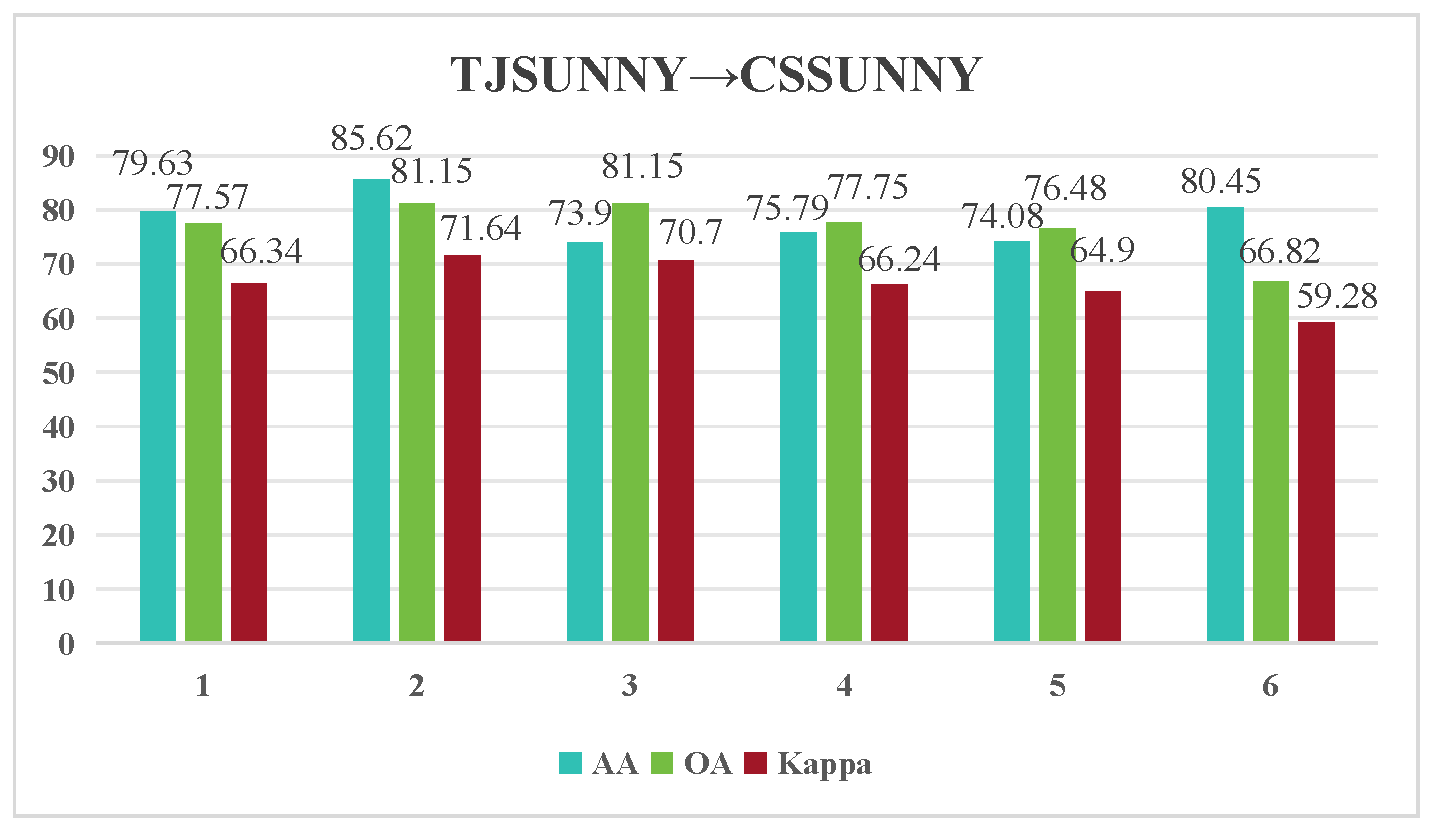
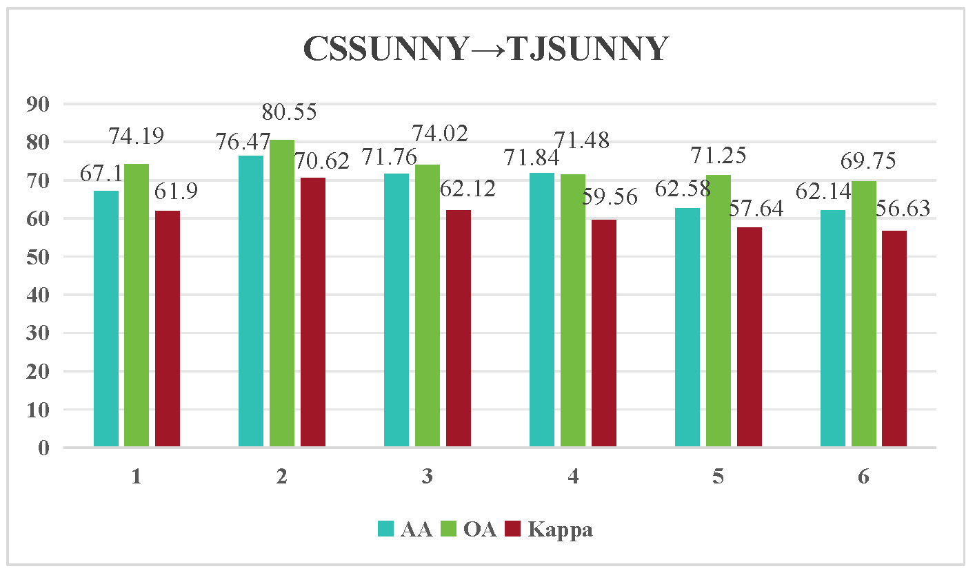
| Class | S-Only | DANN | MDDIA | DABAN | SILDA-VC | CDS | PCS | PCS+SDM | PCS+BMD | RBPCL |
|---|---|---|---|---|---|---|---|---|---|---|
| 1 | 34.02 | 55.59 | 53.88 | 55.59 | 65.48 | 64.07 | 60.33 | 48.98 | 67.64 | 70.73 |
| 2 | 53.67 | 79.46 | 47.71 | 79.46 | 7.12 | 38.26 | 61.14 | 57.05 | 35.61 | 43.4 |
| 3 | 98.66 | 53.85 | 95.97 | 53.85 | 64.88 | 71.48 | 52.35 | 86.29 | 56.86 | 50.17 |
| 4 | 46.45 | 96.72 | 91.76 | 96.72 | 93.99 | 100 | 95.05 | 76.5 | 80.87 | 93.44 |
| 5 | 42.7 | 47.29 | 66.17 | 47.28 | 63.57 | 74.72 | 79.11 | 93.39 | 89.59 | 98.1 |
| 6 | 100 | 100 | 100 | 100 | 100 | 100 | 100 | 100 | 100 | 100 |
| AA | 62.59 | 72.15 | 75.92 | 72.15 | 65.84 | 74.75 | 74.66 | 77.03 | 71.76 | 76.47 |
| OA | 41.55 | 54.84 | 60.32 | 54.84 | 59.54 | 67.1 | 69.19 | 70.86 | 74.41 | 80.55 |
| Kappa | 28.28 | 43.29 | 43.36 | 43.29 | 43.72 | 52.91 | 56.67 | 58.62 | 62.6 | 70.62 |
| Class | S-Only | DANN | MDDIA | DABAN | SILDA-VC | CDS | PCS | PCS+SDM | PCS+BMD | RBPCL |
|---|---|---|---|---|---|---|---|---|---|---|
| 1 | 29.75 | 30.61 | 11.85 | 32.59 | 51.61 | 26.96 | 28.9 | 58.34 | 68.4 | 62.82 |
| 2 | 40.55 | 99.97 | 100 | 40.12 | 100 | 100 | 100 | 100 | 100 | 47.74 |
| 3 | 34.97 | 2.16 | 34.8 | 97.75 | 21.57 | 37.3 | 48.21 | 22.4 | 42.8 | 69.28 |
| 4 | 49.71 | 12.79 | 37.06 | 73.68 | 9.43 | 33.85 | 48.61 | 33.11 | 62.72 | 92.69 |
| 5 | 98.43 | 79.72 | 100 | 98.74 | 67.95 | 100 | 100 | 92.58 | 47.12 | 100 |
| 6 | 41 | 96 | 86 | 97 | 85 | 100 | 97 | 82 | 94 | 97 |
| AA | 49.07 | 53.54 | 61.62 | 73.31 | 55.92 | 66.35 | 70.45 | 64.74 | 69.17 | 78.26 |
| OA | 47.05 | 51.66 | 51.94 | 55.41 | 59.55 | 58.38 | 61.29 | 69.08 | 69.12 | 69.69 |
| Kappa | 35.53 | 39.86 | 43.06 | 46.07 | 47.6 | 49.63 | 52.99 | 58.92 | 59.47 | 60.65 |
| Class | S-Only | DANN | MDDIA | DABAN | SILDA-VC | CDS | PCS | PCS+SDM | PCS+BMD | RBPCL |
|---|---|---|---|---|---|---|---|---|---|---|
| 1 | 16.3 | 44.94 | 18.35 | 33.35 | 32.76 | 54.91 | 62.76 | 73.22 | 50.28 | 71.85 |
| 2 | 24.02 | 31.03 | 13.26 | 30 | 22.83 | 28.27 | 52.83 | 58.89 | 70.96 | 87.7 |
| 3 | 25.93 | 31.85 | 37.04 | 69.3 | 34.44 | 76.58 | 44.44 | 99.26 | 65.43 | 77.78 |
| 4 | 100 | 58.82 | 94.12 | 100 | 100 | 92.83 | 100 | 99.58 | 32.07 | 76.47 |
| 5 | 49.8 | 35.33 | 91.29 | 58.12 | 76.18 | 39.25 | 40.18 | 25.5 | 90.47 | 37.69 |
| 6 | 100 | 100 | 100 | 67.5 | 100 | 100 | 100 | 80.49 | 100 | 100 |
| AA | 52.67 | 50.33 | 59.01 | 59.71 | 61.03 | 65.3 | 66.7 | 72.82 | 68.2 | 75.25 |
| OA | 28.18 | 41.3 | 39.76 | 41.85 | 45.19 | 49.75 | 56.26 | 60.27 | 63.06 | 64.38 |
| Kappa | 15.94 | 20.38 | 27.99 | 30.46 | 33.64 | 32.06 | 40.15 | 43.08 | 48.23 | 49.04 |
Disclaimer/Publisher’s Note: The statements, opinions and data contained in all publications are solely those of the individual author(s) and contributor(s) and not of MDPI and/or the editor(s). MDPI and/or the editor(s) disclaim responsibility for any injury to people or property resulting from any ideas, methods, instructions or products referred to in the content. |
© 2025 by the authors. Licensee MDPI, Basel, Switzerland. This article is an open access article distributed under the terms and conditions of the Creative Commons Attribution (CC BY) license (https://creativecommons.org/licenses/by/4.0/).
Share and Cite
Tang, X.; Shi, H.; Li, C.; Jiang, C.; Zhang, X.; Zeng, L.; Zhou, X. Few-Shot Unsupervised Domain Adaptation Based on Refined Bi-Directional Prototypical Contrastive Learning for Cross-Scene Hyperspectral Image Classification. Remote Sens. 2025, 17, 2305. https://doi.org/10.3390/rs17132305
Tang X, Shi H, Li C, Jiang C, Zhang X, Zeng L, Zhou X. Few-Shot Unsupervised Domain Adaptation Based on Refined Bi-Directional Prototypical Contrastive Learning for Cross-Scene Hyperspectral Image Classification. Remote Sensing. 2025; 17(13):2305. https://doi.org/10.3390/rs17132305
Chicago/Turabian StyleTang, Xuebin, Hanyi Shi, Chunchao Li, Cheng Jiang, Xiaoxiong Zhang, Lingbin Zeng, and Xiaolei Zhou. 2025. "Few-Shot Unsupervised Domain Adaptation Based on Refined Bi-Directional Prototypical Contrastive Learning for Cross-Scene Hyperspectral Image Classification" Remote Sensing 17, no. 13: 2305. https://doi.org/10.3390/rs17132305
APA StyleTang, X., Shi, H., Li, C., Jiang, C., Zhang, X., Zeng, L., & Zhou, X. (2025). Few-Shot Unsupervised Domain Adaptation Based on Refined Bi-Directional Prototypical Contrastive Learning for Cross-Scene Hyperspectral Image Classification. Remote Sensing, 17(13), 2305. https://doi.org/10.3390/rs17132305