Underwater Sound Speed Profile Inversion Based on Res-SACNN from Different Spatiotemporal Dimensions

Abstract

The sound speed profile (SSP) is an important feature in the field of ocean acoustics. The accurate estimation of SSP is significant for the development of underwater position, communication, and associated fundamental marine research. The Res-SACNN model is proposed for SSP inversion based on the convolutional neural network (CNN) embedded with the residual network and self-attention mechanism. It combines the spatiotemporal characteristics of sea level anomaly (SLA) and sea surface temperature anomaly (SSTA) data and establishes a nonlinear relationship between satellite remote sensing data and sound speed field by deep learning. The single empirical orthogonal function regression (sEOF-r) method is used in a comparative experiment to confirm the model’s performance in both the time domain and the region. Experimental results demonstrate that the proposed model outperforms sEOF-r regarding both spatiotemporal generalization ability and inversion accuracy. The average root mean square error (RMSE) is decreased by 0.92 m/s in the time-domain experiment in the South China Sea, and the inversion results for each month are more consistent. The optimization ratio hits 71.8% and the average RMSE decreases by 7.39 m/s in the six-region experiment. The Res-SACNN model not only shows more superior inversion ability in the comparison with other deep-learning models, but also achieves strong generalization and real-time performance while maintaining low complexity, providing an improved technical tool for SSP estimation and sound field perception.

1. Introduction

The sound speed profile (SSP) plays a critical role in determining sound wave propagation characteristics in marine environments [1], significantly influencing underwater acoustic communication [2] and navigation systems [3]. Due to SSP fluctuations, sound waves in heterogeneous water columns experience intricate physical phenomena such as refraction, reflection, and waveguide effects. With advancements in ocean acoustic research, SSP estimation methodologies have evolved from traditional conductivity–temperature–depth (CTD) in situ measurements to modern inversion techniques utilizing sea surface parameters. Carnes et al. [4] established that sea surface temperature (SST) and sea surface height (SSH) contain sufficient information for effective SSP reconstruction, providing a cost-efficient alternative for target marine areas. Among various inversion approaches, the empirical orthogonal function (EOF) method has demonstrated particular efficacy in SSP characterization. Davis [5] mathematically proved that EOF analysis achieves optimal SSP representation through minimum mean square error approximation. Subsequent applications by Shen et al. [6] validated its feasibility in shallow-water environments, while Chen et al. [7] developed the single empirical orthogonal function regression (sEOF-r) technique for global-scale SSP estimation. Although sEOF-r has become predominant in contemporary SSP inversion studies, its performance degrades in spatiotemporal regions with pronounced sound speed gradient variability, particularly in thermocline layers and mesoscale eddy areas where nonlinear ocean dynamics dominate.

The integration of deep learning techniques has introduced novel solutions for enhancing the accuracy of SSP reconstruction. This computational paradigm addresses the inherent limitations of conventional empirical methods in capturing complex spatiotemporal SSP variations. Huang et al. successively proposed a comprehensively optimized back-propagation artificial neural network model [8], a task-driven meta deep learning (TDML) framework [9], and a multi-task learning (MTL) model [10] for spatiotemporal SSP inversion. Using SSPs as input data, they tried various machine learning methods to extract common features of SSPs, enhancing the model’s sensitivity to changes in acoustic field data, improving generalization ability, thereby reducing overfitting effects and improving inversion accuracy.

Subsequently, researchers also applied deep learning methods to SSP inversion. Feng et al. [11] proposed a novel sound speed inversion method based on multi-source ocean remote sensing observations and machine learning, which adapts to large-scale sea regions. Liu et al. [12] proposed for the first time to use a combination of sEOF and generalized regression neural network (GRNN) to inverse SSPs in the Luzon Strait using satellite remote sensing data. Zhao et al. [13] proposed a method for the inversion of the SSP of the South China Sea based on a long short-term memory model. In recent years, there have been an endless stream of artificial intelligence methods for SSP inversion, and they have all demonstrated relatively high inversion accuracy. (As shown in

Table 1. Use of artificial intelligence methods to inverse SSP.

Researchers	Models/Methods	Datasets/Resources	Research Region
Zhang et al. [19]	CNN-BiLSTM-Attention network	Argo gridded dataset	Western Pacific Ocean
Cui et al. [20]	Adaptive sound velocity profile prediction method premised on deep reinforcement learning (DRL-ASP)	Measured dataset	the South China Sea Arctic Ocean Southern Ocean
Qin et al. [21]	Grouped dilated convolution (GDC)	Argo gridded dataset EOF decomposition data Geographic location Temporal information Historical SSP data	Andaman Sea South China Sea Red Sea Western Pacific Ocean
Lu et al. [22]	Hierarchical long short-term memory (H-LSTM) neural network	Argo gridded dataset Ocean experiments dataset	South China Sea
Ou et al. [23]	Random forest (RF)	SSTA(NOAA) SSHA(AVISO) WOA13 dataset Argo dataset	South China Sea

) Other deep learning-based SSP inversion methods include matched field processing (MFP) [14], compressed sensing (CS) [15,16], and feedforward neural networks (FNNs) [17,18]. Although the above various methods can show good SSP inversion accuracy in their specified regions, few researchers have conducted studies on the spatial-temporal generalization performance of artificial intelligence models on a global scale.

At the same time, with the development of ocean data, research on multi-source data fusion has gradually deepened. Ou et al. [24] proposed an SSP reconstruction method based on the extensible end-to-end tree boosting (XG-Boost) model. By combining satellite remote sensing data and Argo profile data, they extracted the feature matrix of SSP. Using root mean square error (RMSE) as the accuracy evaluation index, compared with the sEOF-r model in linear regression methods, the RMSE of the XG-Boost model was reduced by 0.59 m/s. Wu et al. [25] proposed a data-fusion-driven multi-input multi-output convolutional regression neural network (DF-MIMO-RCNN) model. This model combines real-time remote sensing SST based on satellites, historical SSP feature vectors, historical average temperature below the sea surface, and corresponding spatial coordinate information. The model gets rid of the dependence on sonar observation data and can be applied to a wider area. In addition, Yuan et al. [26] used the data from version 2.24 of the ocean data assimilation system (SODA2.24), developed a prediction model for three-dimensional ocean sound speed fields using a spatiotemporal long-short-term memory self-attention model (ST-LSTM-SA) based on deep learning, adopted transfer learning, trained on reanalysis data, and showed good prediction ability by effectively capturing the spatial and temporal changes in sound speed in the ocean.

To improve the generalization ability of the model and alleviate the spatiotemporal sensitivity of SSP inversion, based on sea surface data from remote sensing and Argo profile data, we propose a SSP estimation model based on a convolutional neural network architecture, the Residual Network Self-Attention Mechanism Convolutional Neural Network (Res-SACNN) model. Different from previous research, we not only use a deep learning model for real-time, top-down SSP inversion but also focus on alleviating the failure of SSP inversion in key regions around the global ocean. The main contributions of this paper are as follows:

• By designing a dual-channel CNN architecture, multi-source data fusion with spatiotemporal mismatch is achieved, which extracts spatiotemporal features of sea-surface parameters.
• By integrating the residual network and self-attention mechanism into the CNN framework, a nonlinear mapping model between surface parameters and sound speed field is established, which improves the SSP inversion accuracy.
• By conducting multi-regional and seasonal evaluations of the deep learning model, spatiotemporal generalization capabilities are enhanced, which mitigates the spatiotemporal sensitivity limitations of sEOF-r methods.

The remaining of this paper is organized as follows: Section 2 introduces the data and the Res-SACNN model, Section 3 shows the comparison results of SSP inversion with traditional methods, Section 4 conduct model evaluation, and Section 5 is the summary.

2. Materials and Methods

2.1. Data Preparation and Preprocessing

Constructing a high-quality dataset is the foundation for training deep learning models. Chen et al. [27] proposed that the local sea level anomaly (SLA) plays the dominant role in influencing the reconstruction effect, followed by the sea surface temperature anomaly (SSTA). Therefore, the gridded Argo float data, SLA data, and SSTA data from 2004 to 2018 are used as inputs for this study. The data from 2004 to 2017 are used as training data, and the data from 2018 are used as test data.

The Argo float data are sourced from the Array for Real-time Geostrophic Oceanography. The dataset provides vertical profile information on the ocean’s temperature and salinity structure that has been processed into a grid with a spatial resolution of 1° × 1°, covering global ocean areas from 2000 to 2023. Using the temperature and salinity profile data provided by Argo, we employ the simplified version of the Wilson formula [28], the Medwin formula [29], to calculate the sound speed:

$$C=1449.2+4.6T-0.55T^2+0.00029T^3+\left(1.34-0.01T\right)\left(S-35\right)+0.016D$$

(1)

where C represents the sound speed (in m/s), T represents the temperature (in °C), S represents the salinity (in ‰), and D represents the depth (in m). We select Argo data from January 2004 to calculate the global sound speed by Equation (1). Figure 1 is a schematic diagram of the global monthly mean sea surface sound speed distribution. The global sea surface sound speed shows a distribution characteristic of being high at the equator and low at the poles. The reason is that from the equator to the poles, the solar radiation gradually weakens, and the surface water temperature also gradually decreases, resulting in the sea surface sound speed in the low-latitude areas generally being higher than that in the high-latitude areas.

The SLA data are sourced from the satellite altimetry product data of the French Archiving Validation and Interpretation of Satellite Oceanographic (AVISO). The dataset provides sea surface height information with a spatial resolution of 0.25° × 0.25° and a temporal resolution of weekly, covering the global ocean, which can reflect the SSH changes caused by the ocean dynamic process. Figure 2 is the distribution of global SLA in January 2004.

The SSTA data comes from the SST observation data of the Advanced Very High-Resolution Radiometer (AVHRR) sensor, providing the changing characteristics of the sea surface thermal conditions, with a time from 1981 to 2023. In addition, this study performs interpolation, outlier removal, and grid point matching on the SSTA data converted from SST and SLA data to ensure the availability and uniformity of the data.

In addition, we conduct an innovative exploration in data processing. The SST data and SSH data are uniformly converted into anomaly forms, which are used as the input data for the neural network model. There are significant differences in resolution among Argo data, AVHRR data, and AVISO data, and their forms of physical quantity expression are also different. The SSH data provided by AVISO is presented in the form of anomalies, while AVHRR only provides the original SST data. These differences in data form and resolution pose challenges for the fusion of multi-source data and the training of the neural network model. To enhance the consistency and compatibility of the data, the SST data in this study is also processed into anomaly values. It is mainly divided into the following steps:

• Average the two SST observations of AVHRR per day and store them as the SST data of that day.
• Conduct a separate study for each month. Take the monthly average SST of that month, and subtract the monthly average SST from the SST of that day stored in the previous step to obtain the SSTA of each day.
• Save the SSTA data in a manner of monthly averaging.

This processing method holds significant research importance: Firstly, the utilization of the anomaly form can effectively eliminate the influence of varying physical dimensions, enhancing compatibility and comparability among multi-source data. Secondly, this unified data representation approach substantially improves neural networks’ capability to learn complex oceanic features, thereby optimizing the training process. Thirdly, through standardized preprocessing of input data, the accuracy and reliability of SSP inversion can be significantly enhanced. Figure 3 is the global SSTA distribution in January 2004 derived from AVHRR based on the above three steps.

Considering the impact of the spatial heterogeneity of ocean depth across the globe on the effective depth of the data, a scientific and systematic optimization is carried out for the processing of gridded Argo data. Due to significant variations in sea depth across different ocean regions, the effective depth of Argo float observation data also varies accordingly. To ensure the data’s consistency and integrity, this study adopts a unified depth standard, selecting 58 layers of Argo data corresponding to an effective range of 1975 m as the baseline. However, the sea depth in some areas may be less than 1975 m in practice, resulting in fewer than 58 effective layers of Argo data in these regions. To supplement the Argo data in shallow sea areas, we introduce a linear interpolation method. By reasonably interpolating the existing observational data along the vertical depth, the missing depth layer data are completed, ensuring that the Argo data at all grid points reach the uniform standard of 58 layers. This method not only effectively fills data gaps but also retains the physical characteristics of the original data to a certain extent, while better adapting to the training requirements of the neural network model.

Under the deep learning framework, this study takes advantage of the wide coverage and real-time nature of satellite remote sensing data to achieve the modeling of the nonlinear mapping relationship between sea surface parameters and SSP features, thereby significantly improving the accuracy and reliability of SSP inversion. After data preprocessing, we select the gridded Argo data, SLA data, and SSTA data from 2004 to 2018, with both SLA and SSTA using monthly averaged data. The data from all months of the first 14 years were used as the training set for the model, while the data from 2018 were used as the test set. Since SSP exhibits relatively significant seasonal variations, the model output is targeted only at SSPs for specific months, which are then compared with the gridded Argo data to adjust the model performance.

2.2. Single Empirical Orthogonal Function Regression Method

The EOF method has also been continuously optimized. Currently, most researchers use the sEOF-r method to inverse the SSP. Liu et al. [30] used the sEOF-r method to inverse the global SSPs and evaluated the performance at different stations and on a global scale. sEOF-r is a method for analyzing structural features in matrix data and extracting the main feature quantities of the data. In this study, the eigenvectors correspond to the spatial structure of the SSP called the spatial mode; the principal components correspond to the temporal distribution of the SSP called the temporal coefficient.

We place the sound speed anomaly profile (SSAP) of a 2° grid within the period from 2004 to 2017 in a matrix Q in chronological order. The dimension of Q is M × N, where M represents the number of depth layers of the SSP, and N is the number of SSAPs placed in the matrix. Perform EOF decomposition on the matrix Q to obtain M EOFs and the corresponding coefficient matrix. Label the m-order EOF as $f_m=\left(m=1,\dots ,M\right)$. First, calculate the cross product of the matrix Q to obtain the covariance matrix R:

$$R=Q\times Q^H$$

(2)

where H represents the conjugate transpose of the matrix. Calculate the eigenvalues and eigenvectors of the covariance matrix R:

$$\left(R-\lambda I\right)F=0$$

(3)

where $F=\left[f_1\cdots f_M\right]$ is the empirical orthogonal matrix, $\lambda =diag\left({\lambda }_1,\dots ,{\lambda }_M\right)$ is the coefficient matrix, and ${\lambda }_m\left(m=1,\dots ,M\right)$ is the m-order EOF coefficient. Since the total weight proportion of the 4-order EOF coefficients is greater than 92% [27], the SSAP can be described by the linear combination of the 4-order EOFs, written as

$$SSAP={\alpha }_0+{\displaystyle \sum _{m=1}^4{\alpha }_m{f}_m,m=0,1,\cdots ,4}$$

(4)

where ${\alpha }_m$ is the linear combination coefficient of the m-order EOF, and ${\alpha }_0$ is the constant coefficient.

By combining with the known sea surface database, a regression relationship between the sea surface data and the sEOF-r coefficients is established, and SSP inversion is performed through this regression relationship.

2.3. Res-SACNN Model

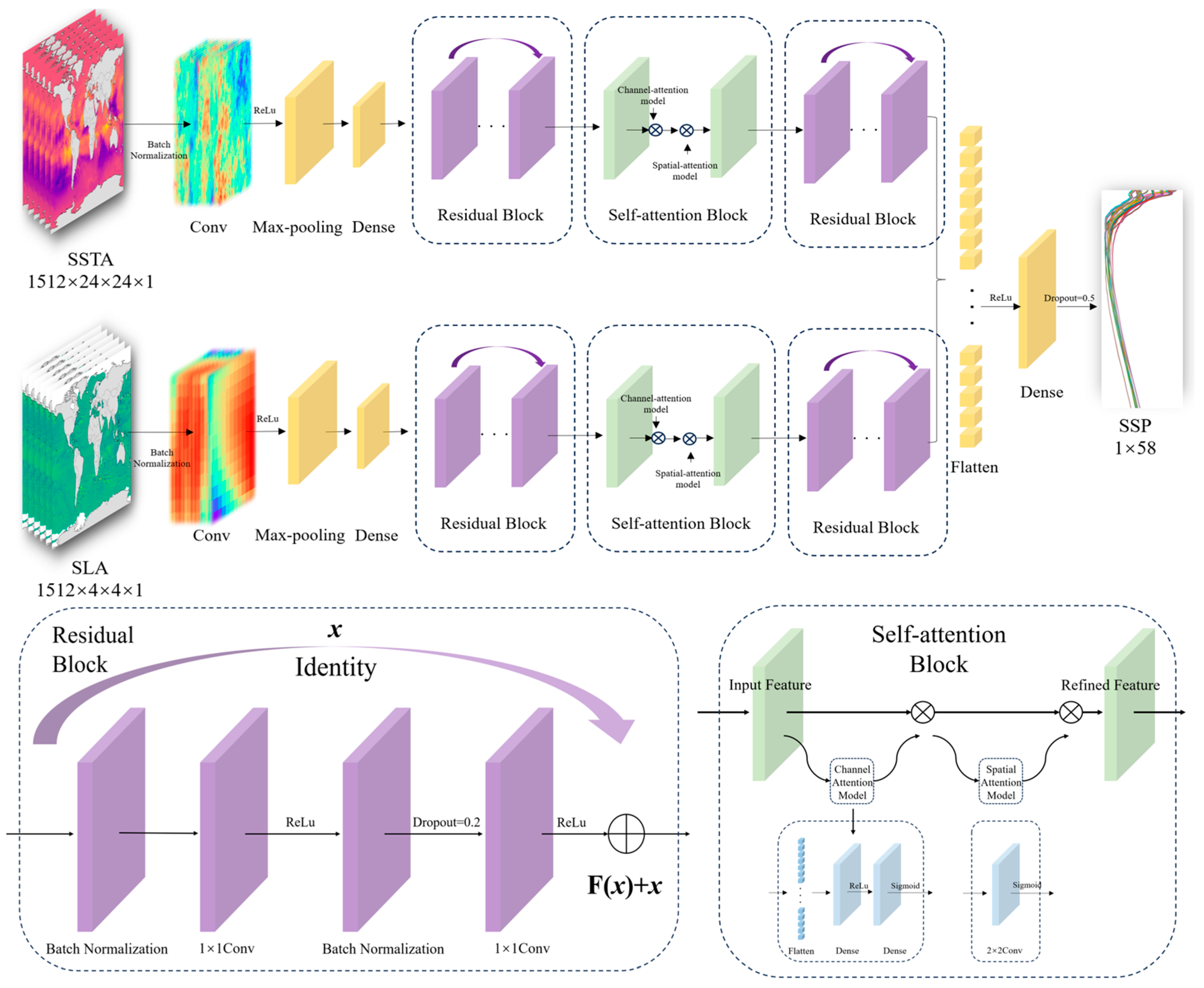
2.3.1. Construction of the Res-SACNN Model

This study aims to explore an SSP inversion method based on CNN to improve inversion accuracy and efficiency while alleviating the spatiotemporal sensitivity of traditional inversion methods. CNN has achieved remarkable results in fields such as image processing [31] and object detection [32]. To inverse the SSP and establish a nonlinear relationship between sea-surface-related parameters and underwater SSPs, this study integrates multi-source satellite remote sensing data and uses the CNN model to extract spatial features representing different sea surface parameters. We call it the Res-SACNN model. Figure 4 shows the structure of the Res-SACNN model.

The Res-SACNN model is designed in this study (the residual network and the self-attention mechanism are added based on the CNN model), with inputs being multi-layer SSTA and SLA, and output of one training being an SSP (the output of one experiment is SSPs at 9 points within a horizontal spatial range of 2° × 2°). For multi-source data with different resolutions, the main approach in this study is to use dual-channel input, separately processing SSTA and SLA, establishing two parallel CNNs, and then merging the two channels to achieve multi-source data fusion. Each sub-channel includes convolutional layers, pooling layers, and embeds two residual networks and one self-attention mechanism. The residual network block includes two layers of batch normalization and two layers of convolution, where the ReLU activation function is used. The self-attention mechanism block consists of channel attention and spatial attention. For channel attention, it first passes through a flatten layer and then two fully connected layers, with the activation functions being ReLU and Sigmoid, respectively. The spatial attention mainly uses a dilated convolution layer to increase the receptive field, and finally outputs through the Sigmoid activation function (As shown in

Table 2. Hyperparameter settings of Res-SACNN.

	Hyperparameter	Value
Residual Block	Kernel size	(1, 1)
	Strides	1
	Learning rate	0.001
	Dropout	0.2
Self-attention Block	Reduction	8
	Kernel size	(2, 2)
	Strides	1
	Learning rate	0.0001
	Dilation rate	2
Res-SACNN Fitting	Epochs	2000
	Batch-size	64
	Early Stopping Patience	40

). Considering the differing degrees of influence of SSTA and SLA on SSP inversion, this paper assigns different weights to the two channels, determining that SLA: SSTA = 1.50:1.00, and finally merges the channel outputs to inverse the SSP with 58 layers.

Additionally, the Adam optimizer and mean squared error (MSE) loss function are used, along with early stopping and learning rate decay strategies to prevent overfitting during the training process.

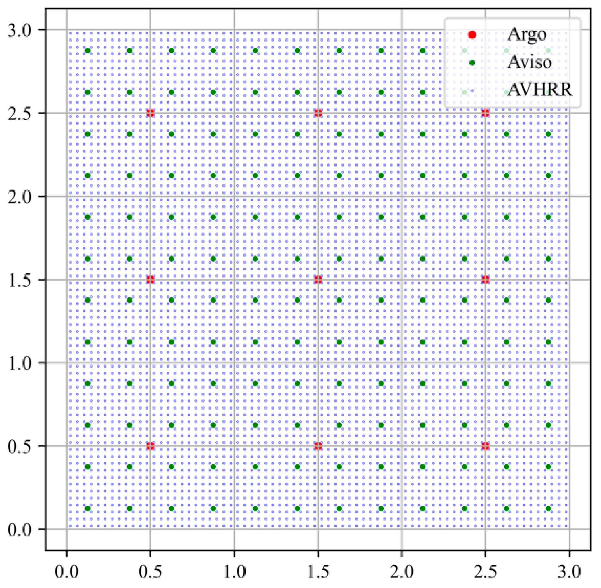
2.3.2. Multi-Source Data Fusion

Considering the limitations of a single data source, we adopt multi-data fusion technology to effectively integrate various types of sea surface data. By designing a specialized feature extraction network and fusion strategy, the accuracy of feature extraction and the precision and generalization performance of SSP inversion are improved. After obtaining multi-source data, the data itself is processed first. For sea surface data, there are phenomena such as data missing and data anomalies. In this study, the multi-source data are all corrected. At the same time, to achieve the fusion of multi-source data, grid point matching is carried out for data with different resolutions, the grid matching forms of various data are observed, and then the data matching method is determined. Figure 5 is the multi-source data grid point diagram, which demonstrates grid point matching for Argo data, AVHRR data, and AVISO data. This process ensures the consistent expression of each data type at the same grid point through the precise matching of the three types of data in the spatial dimension. The main data fusion method in this paper is reflected in the construction of the model architecture.

Table 3. The dual-channel hyperparameter settings for multi-source data processing.

Layer	SLA Channel				SSTA Channel
	Input	Type	HP	Output	Input	Type	HP	Output
1	(1512, 4, 4, 1)	Batch Normalization	/	(1512, 4, 4, 1)	(1512, 24, 24, 1)	Batch Normalization	/	(1512, 24, 24, 1)
2	(1512, 4, 4, 1)	Conv2D	(1, 1)	(1512, 4, 4, 64)	(1512, 24, 24, 1)	Conv2D	(1, 1)	(1512, 24, 24, 128)
3	(1512, 4, 4, 64)	MaxPool2D	(2, 2)	(1512, 2, 2, 64)	(1512, 24, 24, 128)	MaxPool2D	(3, 3)	(1512, 8, 8, 128)
4	(1512, 2, 2, 64)	Dense	Relu	(1512, 2, 2, 32)	(1512, 8, 8, 64)	Dense	Relu	(1512, 8, 8, 32)
5	(1512, 2, 2, 32)	Batch Normalization	/	(1512, 2, 2, 32)	(1512, 8, 8, 32)	Batch Normalization	/	(1512, 8, 8, 32)
6	(1512, 2, 2, 32)	Residual block	/	(1512, 2, 2, 64)	(1512, 8, 8, 64)	Residual block	/	(1512, 8, 8, 128)
7	(1512, 2, 2, 64)	Self-attention block	/	(1512, 2, 2, 64)	(1512, 8, 8, 128)	Self-attention block	/	(1512, 8, 8, 128)
8	(1512, 2, 2, 64)	Residual block	/	(1512, 2, 2, 64)	(1512, 8, 8, 128)	Residual block	/	(1512, 8, 8, 128)
9	(1512, 2, 2, 64)	GlobalAveragePooling2D	/	(6048, 64)	(1512, 8, 8, 128)	GlobalAveragePooling2D	/	(96,768, 128)

gives the hyperparameter (HP) settings of the two channels in the Res-SACNN model. To ensure that the data dimensions can be unified after passing through the sub-channels and adapting to the post-merging channel operation, we adjust the hyperparameters of the two sub-channels in the settings of the convolutional layer and the pooling layer setting. At the same time, the ability to extract the spatial features of the data is strengthened through the custom residual network module and the self-attention mechanism, respectively.

2.3.3. The Training Process of the Res-SACNN Model

The performance of the Res-SACNN model in the inversion of the SSPs is optimized by adjusting the network architecture of the CNN, the activation functions of each layer, and the hyperparameters of the two parallel channels. Regarding the SSP inversion at a certain point with a resolution of 1° × 1°, the SSTA corresponds to 24 × 24 valid points, and the SLA corresponds to 4 × 4 valid data points. Generally, the CNN model is used to handle image problems, and the input matrix is mostly 256 × 256, with more obvious data features. Therefore, the CNN model needs to be changed in terms of the number of layers and the number of iterations in this study; otherwise, overfitting and non-convergence at the end are prone to occur. In the process of optimizing the architecture, this study starts from the direction of fewer layers and fewer iterations to ensure that more complete features can be extracted and the phenomenon of being sensitive to outliers can be prevented. The training process of this model mainly includes the following six steps:

• Data Normalization: Normalization processing is a common data preprocessing method in machine learning. Due to the different magnitudes and large data values of the three types of data, SLA, SSTA, and SSP, to ensure the convergence of the model, we use the Min–Max normalization method to constrain the training data within the [0, 1] interval to facilitate the effect of feature extraction. The normalization calculation formula is as follows:

  $$X^{\prime }=\left(X-X_{\min }\right)/\left(X_{\max }-X_{\min }\right)$$

  (5)

  where $X^{\prime }$ is the normalized datais the normalized data, X is the original data, $X_{\min }$ is the minimum value of the original data, and $X_{\max }$ is the maximum value of the original data.
• Feature Extraction: We use convolution operations and max-pooling operations to extract features from SLA and SSTA. The convolution operation is mainly used to extract local features from the input data, and the max-pooling operation is a down-sampling method that captures local patterns by sliding the convolution kernel to generate multi-level feature representations; then, the down-sampling operation is used to reduce redundant information and enhance the translation invariance and robustness of the features. In this model, the data sizes of SLA and SSTA are different. Therefore, in the process of feature extraction, different convolution kernels and pooling kernels are adopted for the two channels for feature extraction.
• Residual Network Module [33]: The design of the residual network module is an important part of this model. Its structure contains two convolutional layers and two batch normalization layers. In this module, we also introduce a regularization layer to reduce the dependence between neurons and thereby effectively suppress the occurrence of overfitting. The generalization ability of the model can be improved, making it more adaptable and stable when dealing with complex data.
• Self-Attention Mechanism [34]: This mechanism mainly consists of two core modules, the channel module and the spatial module. Among them, the core structure of the channel module includes one unfolding layer and two fully connected layers. This design can effectively capture the global information association between different channels, thereby enhancing the richness of feature expression. The spatial module is implemented by a convolutional layer with a convolution kernel size of 2 × 2, which is mainly used to extract local spatial features and capture the spatial dependence between pixels. These two modules work together to enable the model to better understand the feature distribution of the input data on multiple scales.
• Dual-Channel Weight Setting: In the design of this model, differentiated weight settings are made for the dual-channel data (SLA and SSTA). SLA is a key input variable and plays a more important role in the SSP inversion process [27], and its impact on the model performance is particularly significant; while SSTA also provides valuable information, but its role is relatively more auxiliary. Based on this characteristic, we assigned different weights to SLA and SSTA and set the weight ratio of the two to 1.5:1. This design highlights the dominant position of SLA, while taking into account the supplementary role of SSTA, thereby more effectively capturing the complex nonlinear relationship between sea surface parameters and SSP.
• Model Evaluation: In order to comprehensively and objectively reflect the inversion performance of this model, we use MSE as the loss function and RMSE as the error indicator. The calculation formulas are as follows:

  $$MSE={\displaystyle \frac{1}{n}}{\displaystyle \sum _{i=1}^n{\left(\widehat{y_i}-y_i\right)}^2}$$

  (6)

  $$RMSE=\sqrt{{\displaystyle \frac{1}{n}}{\displaystyle \sum _{i=1}^n{\left(\widehat{y_i}-y_i\right)}^2}}$$

  (7)

  where $y_i$ is the true value, and $\widehat{y_i}$ is the predicted value.

3. Results

3.1. Experimental Design

To comprehensively evaluate the generalization performance of the Res-SACNN model across different spatiotemporal dimensions, we select six regions for comparative experiments: the Northwest Pacific (35°N, 145°E), the Northwest Atlantic (30°N, 130°W), the Cape of Agulhas region (38°S, 15°E), the Tasman Sea off eastern Australia (40°S, 160°E), eastern South America (45°S, 130°W), and the South China Sea (17°N, 115°E). These points are marked in Figure 1. Among these, the temperature and salinity characteristics of the target points in the Northwest Atlantic and the South China Sea are relatively stable [35], with smaller sound speed gradients.

In contrast, the other regions are characterized by rich ocean dynamic phenomena. The Northwest Pacific is marked by the strong Kuroshio Current and its extension, frequent mesoscale eddies, and prominent frontal structures during winter and spring [36]. The Cape of Agulhas region is dominated by the high-temperature and high-salinity Agulhas Current, which influences global thermohaline circulation through “Agulhas Leakage” and eddy shedding [37]. The Tasman Sea is driven by the East Australian Current, with active eddies and a subtropical front that exacerbates gradient changes. It is also significantly affected by monsoons and ENSO events [38]. Eastern South America is centered around the Antarctic Circumpolar Current, accompanied by strong gradients from the Subantarctic Front and Polar Front, as well as deep-sea mixing and upwelling phenomena, creating a complex marine environment [39].

Related ocean dynamics research found that significant failures occurred in SSP inversion using the sEOF-r method in the four regions with active dynamic phenomena. Therefore, we focus on the regions where traditional methods fail to systematically evaluate the performance of the Res-SACNN model in SSP inversion. At the same time, a detailed comparison of data from different months reveals the spatiotemporal variation patterns of SSP and further validates the sensitivity and accuracy of the Res-SACNN model in capturing these changes. This study conducts experiments mainly from two aspects:

• Experiments in different time domains.

To comprehensively evaluate the performance of the Res-SACNN model in the time dimension, we select data from all months throughout the year to cover the impact of seasonal variations on the SSP. Taking the South China Sea as an example, the inversion results of different months are compared and analyzed. The key points to focus on are: whether the model’s performance is stable during periods with significant seasonal changes (such as the transition periods between spring-summer and autumn-winter); the changing trend of the RMSE distribution between different months to verify the model’s sensitivity to temporal dynamic changes; comparing the performance of the sEOF-r method in the same period to highlight the advantages of the Res-SACNN in time series inversion and evaluate the model’s adaptability to different time domains.

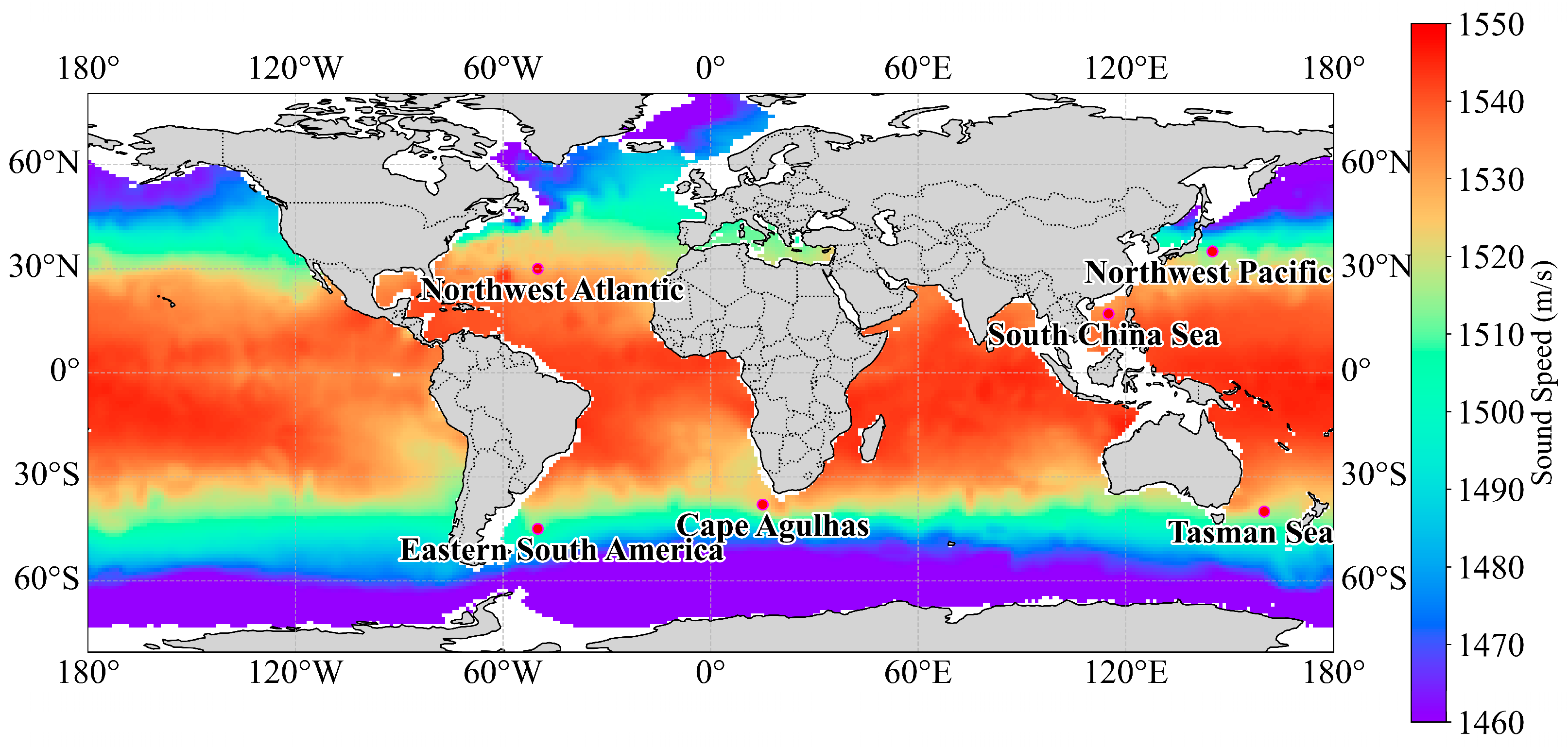
• Experiments in different geographical regions domains.

For the above six regions, we will conduct experiments, respectively, to evaluate the performance of the Res-SACNN model in the spatial dimension. Some of these regions (the Northwest Pacific (35°N, 145°E), the Cape of Agulhas region (38°S, 15°E), the Tasman Sea off eastern Australia (40°S, 160°E), eastern South America (45°S, 130°W)) have complex marine element characteristics and intense dynamic processes, and also include two regions with relatively stable marine environments (the Northwest Atlantic (30°N, 130°W), the South China Sea (17°N, 115°E)). The experimental contents include the following: in each region, evaluating the inversion accuracy of the Res-SACNN model and comparing it with the sEOF-r method to analyze the applicability of the model; verifying the generalization performance of the model in cross-regional applications (that is, whether it can adapt to the marine environment of different regions and maintain a stable high accuracy); combining with actual observed data, exploring the model’s performance in capturing region-specific changes to further prove its reliability in complex environments.

Through the design of the above two experimental directions, we will verify whether the Res-SACNN model has a strong inversion ability and superior generalization performance from different spatiotemporal dimensions, thereby providing a more reliable solution for SSP inversion in complex marine environments.

3.2. Comprehensive Experiments

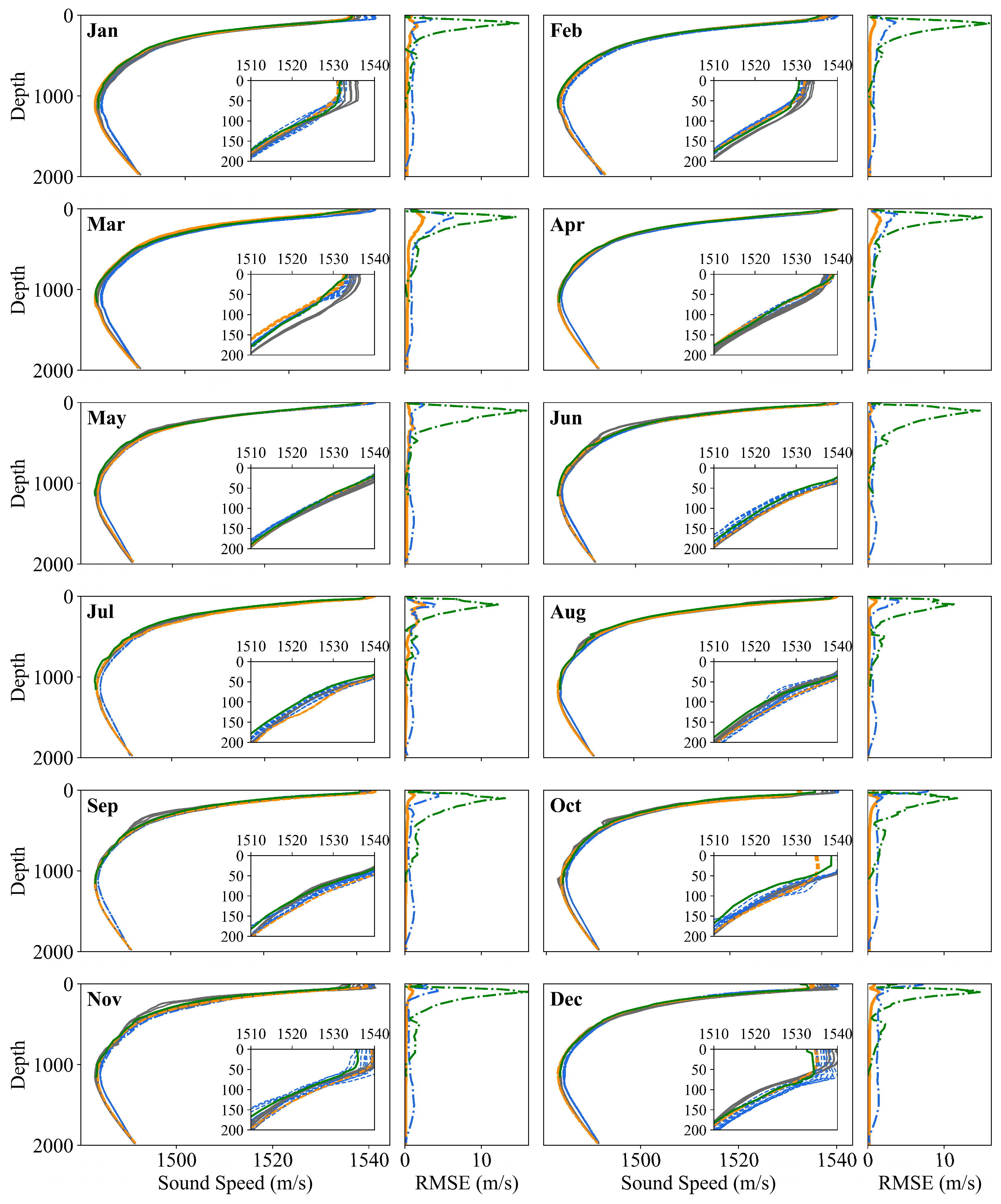
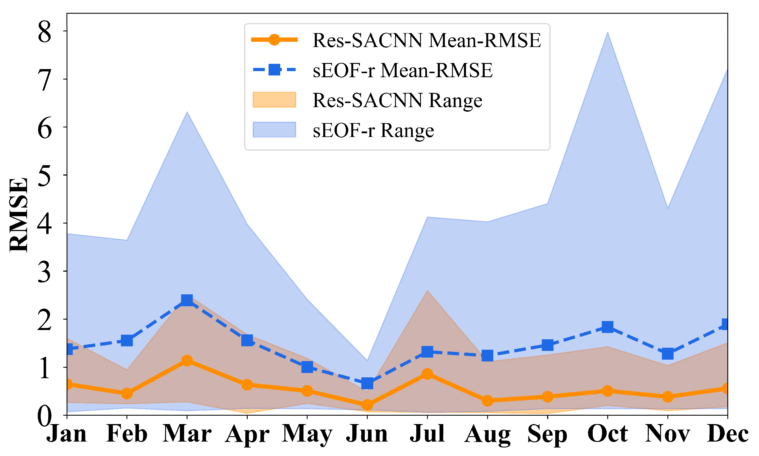
3.2.1. Experiments in Different Time Domains

We select a specific target point in the South China Sea region (115°E, 17°N) and use the Res-SACNN model to carry out the SSP inversion. Among them, a total of nine points near the target point ((114°E, 16°N), (115°E, 16°N), (116°E, 16°N), (114°E, 17°N), (115°E, 17°N), (116°E, 17°N), (111°E, 18°N), (115°E, 18°N), (116°E, 18°N)) are selected for training. The input size is 12 × 14 × 9 = 1512, where 12 refers to 12 months, 14 refers to a total of 14 years from 2004 to 2017, and 9 refers to the central point and the surrounding 9 points. Therefore, the model outputs 9 SSPs within the 2° × 2° spatial range at the same time. To further verify the performance of the model, the sEOF-r method also performs feature extraction and inversion on 9 SSPs at once.

In addition, we also compare the effect of estimating SSPs using World Ocean Atlas 2018 (WOA18) without inversion algorithms. The WOA18 is a global ocean environment dataset released by the National Oceanic and Atmospheric Administration (NOAA) of the United States, which provides long-term statistical average values and time series data of key parameters such as ocean temperature, salinity, dissolved oxygen, and nutrients within a global scope. It covers historical observation records from 1955 to 2017, with a resolution of 1° × 1° and a maximum depth layer of 1500 m. Figure 6 is the comparison of the SSP inversion results between the Res-SACNN model and the sEOF-r algorithm in the South China Sea region in 2018. The gray solid line represents the SSP measured by Argo, the green solid line represents the climatological SSP of WOA18, the orange dashed line represents the SSP inversed by the Res-SACNN model, and the blue dashed line represents the sEOF-r method in the first and third columns. The orange solid line represents the RMSE of the SSP inversed by the Res-SACNN model and the measured SSP, and the blue dashed line and the green dashed line represent those of the WOA18 and sEOF-r methods, respectively, in the second and fourth columns. As shown in Figure 6, this model shows a better performance in the sea surface (below 500 m). At the same time, it confirms that climatological data cannot replace the SSP data obtained through inversion. Due to the influence of various complex dynamic processes such as wind stress, heat exchange, ocean current, and tide in the ocean surface layer area, the sound speed changes often show a high degree of spatiotemporal variability [40]. However, even in such a highly dynamic and changing environment, this model can still maintain a high inversion accuracy.

Meanwhile, we use the kernel density estimation graph to show the RMSE distribution of the Res-SACNN model and sEOF-r method in the South China Sea area (Figure 7). From the kernel density estimation results, its overall RMSE distribution is relatively wide, although the sEOF-r method performs reasonably well in some specific months, indicating that this traditional method may suffer from insufficient stability in providing high-quality SSP inversion results. In contrast, the Res-SACNN model demonstrates stronger consistency in SSP inversion in the China region, with significantly lower RMSE. By comparing the two distributions, it can be observed that the RMSE of Res-SACNN is closer to zero regardless of the month, demonstrating higher accuracy. Additionally, the RMSE of this model remains mostly below 3 m/s, while some RMSE values of the sEOF-r method are still above 4 m/s, with the maximum even approaching 10 m/s. In terms of the overall average RMSE, the performance of this model is only about one-third of the sEOF-r method, showing a significant advantage.

We also provide a detailed statistical analysis of the average RMSE for each month (Figure 8). In all months, the changing trend of the overall RMSE of the inversion of the Res-SACNN model shows a similar situation to the traditional sEOF-r method. It can be seen from the above figure that the Res-SACNN model shows obvious advantages: On the one hand, the RMSE value of this model is smaller, indicating that the deviation between its inversion result and the true value is relatively smaller and the inversion accuracy is higher; on the other hand, the fluctuation range of its RMSE is also more minor, which means that the inversion performance of the Res-SACNN model is more stable between different months, and is less affected by external factors or data changes.

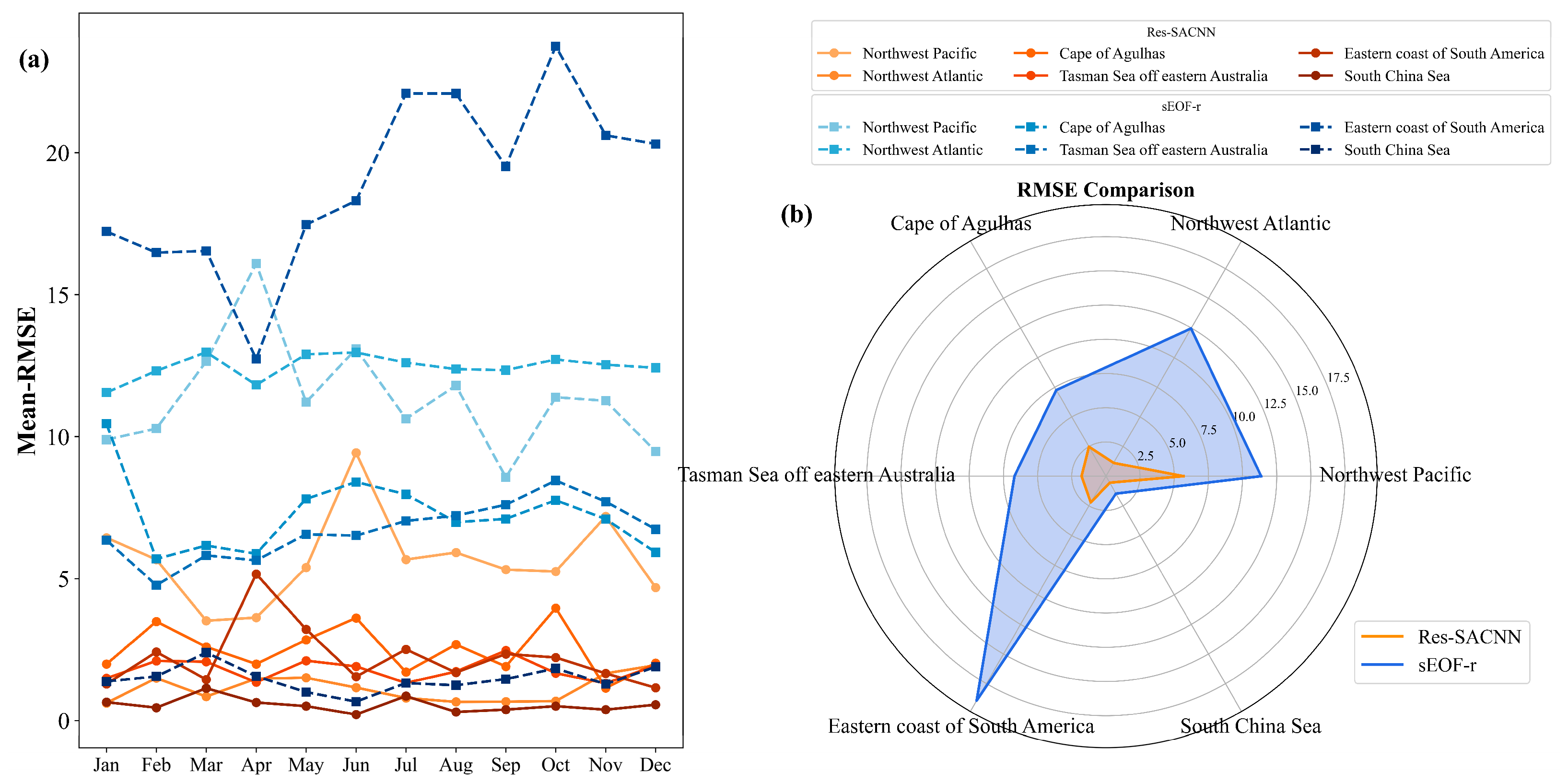
3.2.2. Experiments in Different Regions

To comprehensively verify the performance of the Res-SACNN model in the inversion of the SSP, we select six typical regions for analysis. Figure 9 is the experimental result. The line represents the median of RMSE, the box indicates the main distribution of RMSE, the scatter points are discrete points, the blue represents the sEOF-r method, and the orange represents the Res-SACNN model. Compared with the sEOF-r method, the Res-SACNN model has a lower variance, showing that the variability in its dataset is lower, thereby proving its stronger stability in SSP inverse inference. Moreover, the number of outliers generated by this model is relatively small, which also illustrates the outstanding adaptability of this model in SSP inversion in different time domains and complex marine environments. In the Northwest Atlantic (30°N, 130°W) region, the central point is selected in the sea area far from the continental shelf, where the marine dynamic system is relatively stable and the environmental changes are relatively gentle. Similarly, in the South China Sea (17°N, 115°E) region, due to less influence from strong ocean currents, its marine dynamic characteristics are relatively weak and the external interference is also small. The traditional sEOF-r method has been able to achieve relatively ideal results in such environments that have relatively stable geographical features. However, this model still shows superior performance in these regions, and the RMSE remains below 3 m/s in most cases, further highlighting its high accuracy and stability under different environmental conditions.

According to the regional analysis before the experiment, the Northwest Pacific (35°N, 145°E), the Cape of Agulhas region (38°S, 15°E), the Tasman Sea in the eastern part of Australia (40°S, 160°E), and the eastern part of South America (45°S, 130°W) are regarded as typical regions with highly active marine dynamic systems. The inhomogeneity and drastic changes in the temperature and salinity distribution in these regions bring great difficulties to the SSP inversion. In this case, both the traditional method and this model have failure phenomena in these regions. The RMSE under the sEOF-r method is distributed between 10 m/s and 20 m/s, and the RMSE under the model method also has a distribution exceeding 5 m/s. In general, the performance of the Res-SACNN model is better than the traditional algorithm in various months and different depth layers. The above results indicate that despite the complex marine environment, this model can still provide more reliable and accurate inversion results.

3.3. Experimental Summary

In the process of verifying the SSP inversion performance of the Res-SACNN model, we take the South China Sea region as an example to study the differences in the inversion performance of this model and the sEOF-r method in different months.

Table 4. The RMSE statistical results for all months in the South China Sea of China in 2018, including the maximum, minimum, and average values.

Month	Res-SACNN (m/s)			sEOF-r (m/s)
	Max	Min	Mean	Max	Min	Mean
Jan	1.60	0.27	0.65	3.78	0.07	1.38
Feb	0.95	0.24	0.45	3.64	0.15	1.55
Mar	2.51	0.28	1.14	6.31	0.09	2.39
Apr	1.68	0.04	0.64	3.98	0.14	1.56
May	1.18	0.25	0.51	2.41	0.14	1.00
Jun	0.49	0.07	0.21	1.14	0.11	0.67
Jul	2.59	0.06	0.86	4.13	0.06	1.32
Aug	1.12	0.05	0.30	4.03	0.08	1.24
Sep	1.25	0.04	0.39	4.41	0.14	1.46
Oct	1.43	0.20	0.51	7.97	0.14	1.84
Nov	1.03	0.09	0.38	4.31	0.14	1.28
Dec	1.51	0.18	0.56	7.22	0.14	1.89
Mean	1.45	0.15	0.55	4.44	0.12	1.47

Red represents the maximum value in a column, and green represents the minimum value in a column.

shows the statistical results of the RMSE for all months in the South China Sea. The experimental results show that compared with the sEOF-r method, the Res-SACNN model shows superior stability in the SSP inversion in all months, and the overall average RMSE decreases by 0.92 m/s. The range of RMSE of the Res-SACNN model in each month is significantly smaller. Although the lower bound of RMSE is similar to that of sEOF-r, the upper bound of RMSE fluctuation of this model is 2.99 m/s lower than that of the sEOF-r method. Whether in the case of drastic changes in the SSP in spring and summer, or in the environment where the SSP tends to be gentle in autumn and winter, the Res-SACNN model can maintain a high inversion accuracy and stability. This feature not only verifies the robustness and consistency of the Res-SACNN model under different seasonal conditions, but also highlights its reliability and efficiency in practical applications.

In addition, we analyze the experimental data of six typical regions to comprehensively compare the performance of this model using the sEOF-r method. These regions cover a variety of scenarios from the active areas of marine dynamics to the relatively stable environments to ensure the comprehensiveness and representativeness of the evaluation results. Figure 10 shows the RMSE of six regions. Figure 10a shows the RMSE statistics for different months, where the blue represents sEOF-r and the orange represents Res-SACNN; Figure 10b shows the annual average RMSE in six areas. Res-SACNN shows a smaller RMSE and has a more stable SSP inversion performance in various months and six regions.

Through a series of analyses and validations of the comparative experimental results, it is clear that the SSP inversion method of the Res-SACNN model demonstrates higher accuracy and reliability compared to the sEOF-r method. At the same time, we use the optimization ratio to measure the improvement degree of the Res-SACNN model. The calculation formula of the optimization ratio is as follows:

$$\beta =\left(1-\sqrt{{\displaystyle \frac{{\displaystyle \sum _{i=1}^n{\left(y_i^{\ast }-y_i\right)}^2}}{{\displaystyle \sum _{i=1}^n{\left(y_i-y_i\right)}^2}}}}\right)\times 100\%$$

(8)

where $\beta$ is the optimization ratio, $y^{\ast }$ is the inversion result of this model, and y is the inversion result of the sEOF-r method. In the experiments, the two methods are applied to datasets from different geographical regions and across varying time spans for comparative analysis.

Table 5. Statistical results of RMSE in six regions. ‘Decrease’ represents the reduction in RMSE of the Res-SACNN model relative to the sEOF-r method.

Region	Optimization Ratio	Decrease
Northwest Pacific	50.1%	5.69
Northwest Atlantic	91.0%	11.34
Cape of Agulhas region	65.7%	4.78
Tasman Sea off eastern Australia	73.3%	4.91
Eastern coast of South America	88.3%	16.71
South China Sea	62.5%	0.92
Mean	71.8%	7.39

Red represents the maximum value in a column, and green represents the minimum value in a column.

shows the statistical results of the RMSE for the six regions.

This model can show a better inversion accuracy in different regions. Compared with the traditional sEOF-r method, the RMSE of this model decreases by 11.33 m/s, and the optimization ratio is as high as 91.0% in the Northwest Atlantic region. At the same time, from the statistical results of the six regions, the RMSE of the Res-SACNN model decreases by an average of 7.39 m/s, and the average optimization ratio is 71.8%. The results show that the Res-SACNN model can not only adapt to diverse environmental conditions and maintain a stable performance output but also shows excellent generalization ability. Taking the Northwest Pacific, Cape of Agulhas region, Tasman Sea off eastern Australia and Eastern coast of South America as examples, in the spatiotemporal range with a large sound speed gradient such as the areas where the sound speed distribution is complex due to the drastic changes in temperature, salinity or depth, the inversion ability of the Res-SACNN model is outstanding, and its performance is significantly better than the sEOF-r method, and the optimization ratio can reach more than 50%. At the same time, in the area where the ocean dynamic environment changes gently (South China Sea), this model can also show a better inversion result.

Furthermore, we do not conduct a detailed study on other sea areas affected by factors such as terrain, mesoscale eddies, and ocean currents. The influence of various environmental factors on SSP inversion has not been studied either. This study focuses on the research of the sound field, thereby providing theoretical assistance for underwater target detection and underwater communication. Therefore, research related to practical applications is also one of our future research directions.

In contrast, although the sEOF-r method can also provide a more reasonable inversion result in some simple scenarios, it is powerless in dealing with complex nonlinear features and is prone to large errors due to the influence of data distribution characteristics. With its strong feature extraction ability and nonlinear mapping characteristics, the Res-SACNN model can accurately capture the subtle change rules in the SSP, thereby significantly improving the accuracy and robustness of the inversion results.

4. Discussion

4.1. Model Evaluation

Machine learning has developed rapidly in the field of SSP inversion, and many models have also achieved good inversion results. We use the generalized regression neural network (GRNN) [12] as the comparison object for the evaluation experiment of Res-SACNN. The GRNN model is mainly used to establish a nonlinear mapping relationship between sea surface parameters (SLA and SSTA) and SSP. During its use, the coefficients need to be obtained first using the sEOF method, then these coefficients are input into the GRNN model, and finally the SSP is output. Taking the South China Sea as an example, we used different methods (WOA18, sEOF-r, GRNN, Res-SACNN) to perform monthly inversion of SSP. To show the overall accuracy of various models, we average the monthly inversion results for the whole year and obtained the final annual average SSP inversion results. Figure 11 shows the measured Argo data, the WOA18 climatological data, the inversion of sEOF-r, the inversion of GRNN, and the inversion of Res-SACNN. Overall, the SSP results of several types of methods can fit the measured Argo data well. However, it is evident that the Res-SACNN model exhibits the highest degree of coincidence with the Argo data in the sea surface region ranging from 0 m to 100 m, especially.

To analyze the necessity of the residual block and the self-attention mechanism block, we also conduct ablation experiments to evaluate Res-SACNN. Meantime, to demonstrate that these two blocks can still maintain the inversion accuracy of the model in marine environments with drastic sound speed variations, we conduct ablation experiments on the six regions selected in the previous text and performed the experiments month by month. To highlight the overall generalization performance of the Res-SACNN model, we finally average the experimental results of the six regions. Figure 12 shows the average RMSE results of the ablation experiments in the six regions throughout the year. The results of the ablation experiment show that after removing the residual module or the self-attention mechanism module from the Res-SACNN model, the inversion error increases significantly. This fully demonstrates the importance and effectiveness of the residual module and the self-attention mechanism module, as well as the synergistic benefits between the two modules. In addition, the four models show similar trends in different seasons, which further indicates that the SSP inversion accuracy has a certain seasonal variation.

Moreover, we evaluate the complexity of each part of the Res-SACNN model, using the number of floating-point operations (FLOPs) [41] and params as indicators. Among them, FLOPs are used to represent time complexity, and params refer to the total number of parameters that need to be trained during model training, which is used to represent space complexity. The calculation formula of the FLOPs is as follows:

$$\mathrm{FLOPs}=2HW\left(C_{in}{K}^2+1\right)C_{out}$$

(9)

where H, W and $C_{in}$ are height, width and number of channels of the input feature map, K is the kernel width, and $C_{out}$ is the number of output channels.

Table 6. Model complexity assessment.

Model	FLOPs (M)	Params (M)
CNN	0.12	0.05
SACNN	1.19	0.07
Res-CNN	4.41	0.16
Res-SACNN	8.67	0.25

shows that the time complexity and space complexity of the Res-SACNN model are at a relatively low level [42]. Therefore, this model can be effectively and conveniently applied in practice.

4.2. Limitations and Future Work

Interpretability has always been a major issue hindering the progress of SSP inversion technology. For deep learning models, it is also difficult to solve the problem of poor interpretability. We will study how to embed physical constraints into deep learning models. One approach is to incorporate physical constraints into the loss function, and another is to learn physical mechanisms through the network directly. The key to these two methods lies in how to find the most appropriate physical constraints and mechanisms. Moreover, the fact that different environments correspond to different physical mechanisms is also a research-worthy problem. Therefore, clustering different sea areas globally and stratifying different depth layers are also part of our future research. Through this method, we can further improve the accuracy and interpretability of the inversion, thereby further enhancing the performance of the model in dynamic and complex ocean environments.

5. Conclusions

As an important part of the research on the ocean acoustic field, more accurate SSP inversion is increasingly needed. This study proposes a Res-SACNN model based on CNN for underwater SSP inversion. The development background of this method is associated with the problem of insufficient inversion accuracy of the sEOF-r method in complex areas with a large sound speed gradient or in marine environments with rich dynamic systems. To solve this problem, the study innovatively proposes the Res-SACNN model, which not only inherits the advantages of the traditional method but also solves the problem of gradient disappearance in the training of deep networks by introducing a residual network; at the same time, it uses the self-attention mechanism to enhance the ability to capture key spatiotemporal features.

Through systematic theoretical analysis and extensive experimental verification, the effectiveness and superiority of this method in SSP inversion are proven. Compared with the sEOF-r method, the Res-SACNN model shows significant advantages in several aspects:

• Improve Inversion Accuracy: The Res-SACNN model shows a significant reduction in RMSE (average of 7.39 m/s) across six ocean regions, with an optimization ratio of 71.8%. Notably, accuracy is exceptional in areas with large sound speed gradients, like the Northwest Pacific and Cape of Agulhas region.
• Strong Generalization: The model performs well in both complex, dynamic environments and stable regions (e.g., South China Sea), achieving a 62.5% optimization ratio, demonstrating adaptability to diverse marine conditions.
• Real-Time and Robust: By integrating residual networks and self-attention mechanisms, the model enhances spatiotemporal feature capture and computational efficiency. Combined with satellite remote sensing data, it ensures real-time response and robust performance in variable marine environments.

In summary, the Res-SACNN model makes up for the shortcomings of the traditional method in a complex environment and provides a new technical means for marine SSP inversion. We will also continue to study the influencing factors of SSP inversion, explore the inversion characteristics of the global sea area, and combine the research results with practical applications such as underwater communication and underwater detection.

References

- Chu, X.; Zhao, F.; Wang, Z.; Qian, Y.; Yang, G. Acoustic Wave Propagation in Depth Evolving Sound Speed Field Using the Lattice Boltzmann Method. Phys. Fluids 2024, 36, 097118. [Google Scholar] [CrossRef]
- Liu, Y.; Chen, C.; Feng, X. Investigating the Reliable Acoustic Path Properties in a Global Scale. Front. Mar. Sci. 2023, 10, 1213002. [Google Scholar] [CrossRef]
- Xue, S.; Li, B.; Xiao, Z.; Sun, Y.; Li, J. Centimeter-level-precision Seafloor Geodetic Positioning Model with Self-structured Empirical Sound Speed Profile. Satell. Navig. 2023, 4, 30. [Google Scholar] [CrossRef]
- Carnes, M.R.; Mitchell, J.L.; de Witt, P.W. Synthetic Temperature Profiles Derived from Geosat Altimetry: Comparison with Air-dropped Expendable Bathythermograph Profiles. J. Geophys. Res. Ocean. 1990, 95, 17979–17992. [Google Scholar] [CrossRef]
- Davis, R.E. Predictability of Sea Surface Temperature and Sea Level Pressure Anomalies over the North Pacific Ocean. J. Phys. Oceanogr. 1976, 6, 249–266. [Google Scholar] [CrossRef]
- Shen, Y.; Ma, Y.; Tu, Q.; Jiang, X. Feasibility of Describing the Sound Speed Profile in Shallow Water via Empirical Orthogonal Function. J. Appl. Acoust. 1999, 18, 21–25. [Google Scholar] [CrossRef]
- Chen, C.; Ma, Y.; Liu, Y. Reconstructing Global Sound Speed Profiles Using Sea Surface Data. Appl. Ocean Res. 2018, 77, 26–33. [Google Scholar] [CrossRef]
- Huang, J.; Luo, Y.; Shi, J.; Ma, X.; Li, Q.-Q.; Li, Y.-Y. Rapid Modeling of the Sound Speed Field in the South China Sea Based on a Comprehensive Optimal LM-BP Artificial Neural Network. J. Mar. Sci. Eng. 2021, 9, 488. [Google Scholar] [CrossRef]
- Huang, W.; Li, D.; Zhang, H.; Xu, T.; Yin, F. A Meta-deep-learning Framework for Spatial-temporal Underwater SSP Inversion. Front. Mar. Sci. 2023, 10, 1146333. [Google Scholar] [CrossRef]
- Huang, W.; Zhou, J.; Gao, F.; Wang, J.; Xu, T. Experimental Results of Underwater Sound Speed Profile Inversion by Few-Shot Multi-Task Learning. Remote Sens. 2023, 16, 167. [Google Scholar] [CrossRef]
- Feng, X.; Tian, T.; Zhou, M.; Sun, H.; Li, D.; Tian, F.; Lin, R. Sound Speed Inversion Based on Multi-Source Ocean Remote Sensing Observations and Machine Learning. Remote Sens. 2024, 16, 814. [Google Scholar] [CrossRef]
- Liu, Y.; Chen, Y.; Chen, W.; Meng, Z. Inversion of Sound Speed Profile in the Luzon Strait by Combining Single Empirical Orthogonal Function and Generalized Regression Neural Network. IEEE Geosci. Remote Sens. Lett. 2024, 21, 1502405. [Google Scholar] [CrossRef]
- Zhao, Y.; Xu, P.; Li, G.; Ou, Z.; Qu, K. Reconstructing the Sound Speed Profile of South China Sea Using Remote Sensing Data and Long Short-term Memory Neural Networks. Front. Mar. Sci. 2024, 11, 1375766. [Google Scholar] [CrossRef]
- Tolstoy, A.; Diachok, O.; Frazer, L. Acoustic Tomography via Matched Field Processing. J. Acoust. Soc. Am. 1991, 89, 1119–1127. [Google Scholar] [CrossRef]
- Choo, Y.; Seong, W. Compressive Sound Speed Profile Inversion Using Beamforming Results. Remote Sens. 2018, 10, 704. [Google Scholar] [CrossRef]
- Li, Q.; Shi, J.; Li, Z.; Luo, Y.; Yang, F.; Zhang, K. Acoustic Sound Speed Profile Inversion Based on Orthogonal Matching Pursuit. Acta Oceanol. Sin. 2019, 38, 149–157. [Google Scholar] [CrossRef]
- Huang, W.; Li, D.; Jiang, P. Underwater Sound Speed Inversion by Joint Artificial Neural Network and Ray Theory. In Proceedings of the Thirteenth ACM International Conference on Underwater Networks & Systems, Shenzhen, China, 3–5 December 2018; Association for Computing Machinery: New York, NY, USA, 2018; pp. 1–8. [Google Scholar] [CrossRef]
- Stephan, Y.; Thiria, S.; Badran, F. Inverting Tomographic Data with Neural Nets. In Proceedings of the Challenges of Our Changing Global Environment Conference, OCEANS’ 95 MTS/IEEE, San Diego, CA, USA, 9–12 October 1995; Volume 3, pp. 1501–1504. [Google Scholar] [CrossRef]
- Zhang, W.; Jin, S.; Bian, G.; Cui, Y.; Peng, C.; Xia, H. A Method for Sound Speed Profile Prediction Based on CNN-BiLSTM-Attention Network. J. Mar. Sci. Eng. 2024, 12, 414. [Google Scholar] [CrossRef]
- Cui, X.; Liu, X.; Li, J.; Li, L.; Jiang, B.; Li, S.; Liu, J. Adaptive Sound Velocity Profile Prediction Method Based on Deep Reinforcement Learning. IEEE Sens. Lett. 2024, 8, 6002704. [Google Scholar] [CrossRef]
- Qin, S.; Zhang, Y.; Chen, Z. An Estimation Method of Sound Speed Profile Based on Grouped Dilated Convolution Informer Model. Front. Mar. Sci. 2025, 12, 1484098. [Google Scholar] [CrossRef]
- Lu, J.; Huang, W.; Zhang, H. Dynamic Prediction of Full-Ocean Depth SSP by a Hierarchical LSTM: An Experimental Result. IEEE Geosci. Remote Sens. Lett. 2024, 21, 1501105. [Google Scholar] [CrossRef]
- Ou, Z.; Qu, K.; Liu, C. Estimation of Sound Speed Profiles Using a Random Forest Model with Satellite Surface Observations. Shock Vib. 2022, 2022, 2653791. [Google Scholar] [CrossRef]
- Ou, Z.; Qu, K.; Shi, M.; Wang, Y.; Zhou, J. Estimation of Sound Speed Profiles Based on Remote Sensing Parameters Using a Scalable End-to-end Tree Boosting Model. Front. Mar. Sci. 2022, 9, 1051820. [Google Scholar] [CrossRef]
- Wu, P.; Zhang, H.; Shi, Y.; Lu, J.; Li, S.; Huang, W.; Tang, N.; Wang, S. Real-time estimation of underwater sound speed profiles with a data fusion convolutional neural network model. Appl. Ocean. Res. 2024, 150, 104088. [Google Scholar] [CrossRef]
- Yuan Liu, Y.; Tang, Q.; Li, J.; Chen, G.; Cai, W. ST-LSTM-SA: A Novel Ocean Sound Velocity Field Prediction Model Based on Deep Learning. Adv. Atmos. Sci. 2024, 41, 1364–1378. [Google Scholar] [CrossRef]
- Chen, W.; Ren, K.; Zhang, Y.; Liu, Y.; Chen, Y.; Ma, L.; Chen, S. Reconstruction of the Sound Speed Profile in Typical Sea Areas Based on the Single Empirical Orthogonal Function Regression Method. J. Mar. Sci. Eng. 2023, 11, 841. [Google Scholar] [CrossRef]
- Wilson, W.D. Equation for the Speed of Sound in Seawater. J. Acoust. Soc. Am. 1960, 32, 1357. [Google Scholar] [CrossRef]
- Medwin, H. Speed of Sound in Water: A Simple Equation for Realistic Parameters. J. Acoust. Soc. Am. 1975, 58, 1318–1319. [Google Scholar] [CrossRef]
- Liu, Y.; Chen, Y.; Meng, Z.; Chen, W. Performance of Single Empirical Orthogonal Function Regression Method in Global Sound Speed Profile Inversion and Sound Field Prediction. Appl. Ocean Res. 2023, 136, 103598. [Google Scholar] [CrossRef]
- Karol, G.; Ivo, D.; Alex, G.; Danilo, J.R.; Daan, W. DRAW: A Recurrent Neural Network for Image Generation. arXiv 2015. [Google Scholar] [CrossRef]
- Fnu, N.; Deepshikha, B.; Deepak, K.; Md, A. From Classical Techniques to Convolution-based Models: A Review of Object Detection Algorithms. In Proceedings of the 2025 IEEE 6th International Conference on Image Processing, Applications and Systems (IPAS), Lyon, France, 9–11 January 2025. [Google Scholar] [CrossRef]
- He, K.; Zhang, X.; Ren, S.; Sun, J. Deep Residual Learning for Image Recognition. In Proceedings of the 2016 IEEE Conference on Computer Vision and Pattern Recognition (CVPR), Las Vegas, NV, USA, 27–30 June 2016. [Google Scholar] [CrossRef]
- Dzmitry, B.; Kyunghyun, C.; Yoshua, B. Neural Machine Translation by Jointly Learning to Align and Translate. arXiv 2014. [Google Scholar] [CrossRef]
- Samanta, D.; Goodkin, N.F.; Karnauskas, K.B. Volume and Heat Transport in the South China Sea and Maritime Continent at Present and the End of the 21st Century. Journal of Geophysical Research. Oceans 2021, 126, e2020JC016901. [Google Scholar] [CrossRef]
- Chen, C.; Yang, K.; Duan, R.; Ma, Y. Acoustic Propagation Analysis with a Sound Speed Feature Model in the Front Area of Kuroshio Extension. Appl. Ocean Res. 2017, 68, 1–10. [Google Scholar] [CrossRef]
- Matano, R.; Combes, V.; Palma, E.D.; Strub, P.T. Circulation and Cross-Shelf Exchanges in the Agulhas Bank Region. J. Geophys. Res. Ocean. 2025, 130, e2023JC020234. [Google Scholar] [CrossRef]
- Iain, M.S.; Jock, W.Y.; Mark, E.B.; Roughan, M.; Everett, J.D.; Brassington, G.B.; Byrne, M.; Condie, S.A.; Hartog, J.R.; Hassler, C.S.; et al. The Strengthening East Australian Current, its Eddies and Biological Effects—An Introduction and Overview. Deep Sea Res. Part II Top. Stud. Oceanogr. 2011, 58, 538–546. [Google Scholar] [CrossRef]
- Alejandro, H.O.; Thomas, W.; Worth, D.N. On the Meridional Extent and Fronts of the Antarctic Circumpolar Current. Deep Sea Res. Part I Oceanogr. Res. Pap. 1995, 42, 641–673. [Google Scholar] [CrossRef]
- Alice, A.; Chiara, S.; Stefano, S. Ocean Sound Propagation in a Changing Climate: Global Sound Speed Changes and Identification of Acoustic Hotspots. Earth’s Future 2022, 10, e2021EF002099. [Google Scholar] [CrossRef]
- Molchanov, P.; Tyree, S.; Karras, T.; Aila, T.; Kautz, J. Pruning Convolutional Neural Networks for Resource Efficient Inference. arXiv 2017. [Google Scholar] [CrossRef]
- Tan, M.; Le, Q. Efficient-Net: Rethinking Model Scaling for Convolutional Neural Networks. arXiv 2019. [Google Scholar] [CrossRef]