Abstract
Dissolved oxygen (DO) is a fundamental water quality parameter that directly determines aquaculture productivity. China contributes 57% of the global aquaculture production, with the Guangdong–Hong Kong–Macao Greater Bay Area (GBA) serving as a key contributor. However, this region faces significant environmental challenges due to increasing intensive stocking densities and outdated management practices, while also grappling with the systematic monitoring limitations of large-scale operations. To address these challenges, in this study, a random forest-based model was developed for DO concentration retrieval (R2 = 0.82) using Landsat 8/9 OLI imagery. The Lindeman, Merenda, and Gold (LMG) algorithm was applied to field data collected from four cities—Foshan, Hong Kong, Huizhou, and Zhongshan—to identify key environmental drivers to the changes in DO concentration in these cities. This study also employed satellite imagery from multiple periods to analyze the spatiotemporal distribution and trends of DO concentrations over the past decade, aiming to enhance understanding of DO variability. The results indicate that the average DO concentration in fishponds across the GBA was 7.44 mg/L with a statistically insignificant upward trend. Spatially, the DO levels remained slightly lower than those in other waters. The primary environmental factor influencing DO variations was the pH levels, while the relationship between natural factors such as the temperature and DO concentration was significantly hidden by aquaculture management practices. The further analysis of fishpond water quality parameters across land uses revealed that fishponds with lower DO concentrations (7.293 mg/L) are often located in areas with intensive human intervention, particularly in highly urbanized regions. The approach proposed in this study provides an operational method for large-scale DO monitoring in aquaculture systems, enabling the qualification of anthropogenic influences on water quality dynamics. It also offers scalable solutions for the development of adaptive management strategies, thereby supporting the sustainable management of aquaculture environments.
1. Introduction
Global population growth and rising dietary demands have positioned aquaculture as one of the fastest-growing food production sectors, with it plays a vital role in ensuring global food security [1]. China, as the world’s largest aquaculture producer, exemplifies this global trend [2,3,4]. However, the intensification of aquaculture practices has led to considerable environmental concerns, with water quality degradation emerging as a critical challenge that threatens the long-term sustainability of the industry [5]. Among various water quality indicators, the dissolved oxygen (DO) is particularly crucial, as its concentration directly influences the physiological health, growth rate, and survival of aquatic organisms. Numerous studies have underscored that maintaining stable DO levels is essential for optimal aquatic productivity [6], while hypoxic conditions (i.e., extremely low DO levels) can severely deteriorate the quality of water, disrupt ecosystem functioning, and jeopardize aquaculture sustainability [7].
Traditional in situ investigations of DO are limited by their high operational costs, restricted spatial coverage, and inability to capture the comprehensive spatial distribution patterns of DO across large geographic regions [8]. In contrast, remote sensing offers a viable alternative, as the DO can be indirectly estimated through its strong association with optically detectable biological processes such as photosynthesis and suspended particulate dynamics [9]. Early efforts to estimate DO concentrations employed simple linear regression models [10,11], although their accuracy was constrained by DO’s non-optically active nature. Subsequent research introduced multivariate regression techniques, incorporating other physical and chemical variables such as the water temperature (WT) and chlorophyll-a (Chl-a) levels to improve models’ performance [12,13,14,15].
In biological procedures, DO is primarily produced through photosynthesis carried out by algae and phytoplankton. The concentration of Chl-a in a body of water, the principal photosynthetic pigment, serves as a direct proxy for the phytoplankton biomass and thus reflects the oxygen-generating capacity of the system [16]. As Chl-a is optically active—absorbing and reflecting light at representative wavelengths—it produces a distinct spectral signature that can be detected by satellite sensors [17]. However, the rate of photosynthesis is regulated by the availability of light, which is often reduced with increases in the total suspended matter (TSM) [18]. The TSM, comprising particles such as sediments, detritus, and plankton, is also an optically active parameter that substantially alters the reflectance of water [19]. Consequently, the spectral signature related to DO is a complex mixture of signals from both oxygen-producing and limiting processes, forming a multifaceted but essential basis for remote sensing applications.
To accurately model the nonlinear, high-dimensional relationships underlying DO dynamics, recent studies have increasingly turned to machine learning techniques. Among these, support vector machine (SVM) have demonstrated strong performance in modeling DO concentrations across diverse water bodies [20,21,22,23]. Ensemble learning approaches, particularly random forest (RF) algorithms, have also gained prominence due to their high predictive performance, robustness against overfitting [24], and capacity to handle complex feature spaces [25]. Numerous studies have validated the applicability of RF models in the retrieval of water quality parameters in environments ranging from local reservoirs to global freshwater systems [26,27,28,29].
Despite the success of machine learning in diverse aquatic environments, its application in DO retrieval for fishponds presents unique challenges. These systems are characterized by small sizes, high anthropogenic influence, and rapid changes in water conditions, which result in nonlinear and non-stationary spectral signals that are difficult to interpret using traditional methods. Therefore, a more sophisticated approach to spectral feature extraction is required to address this complexity.
To fill these gaps, this study integrated empirical mode decomposition (EMD) with machine learning techniques to develop an improved DO retrieval model for DO monitoring in fishponds in the GBA. EMD is a data-adaptive signal processing method that is capable of decomposing complex, non-stationary signals into intrinsic mode functions (IMFs), which represent the embedded oscillatory modes across multiple scales [30]. Compared with traditional methods such as wavelet and Fourier transformation, EMD is more effective in isolating weak signals [31] and reducing noise [32]. EMD has been widely applied across various fields [33], including turbulence analysis [34], neural decoding [35], and mechanical fault monitoring [36].
By coupling EMD with machine learning, this study aims to enhance the accuracy and reliability of satellite-based DO retrieval in intensively managed aquaculture systems. Furthermore, we conduct a comprehensive spatiotemporal analysis of DO variations over the past decade, identifying key environmental drivers that influence DO dynamics. The findings contribute to the broader goal of enabling efficient, scalable, and scientifically informed water quality monitoring, offering valuable insights for sustainable aquaculture management in the GBA and beyond.
2. Materials and Methods
2.1. Study Area
The GBA, located between 21°44′N–24°40′N and 111°35′E–115°38′E, encompasses nine cities in Guangdong Province—Guangzhou, Shenzhen, Dongguan, Zhongshan (ZS), Zhuhai, Foshan (FS), Huizhou (HZ), Jiangmen, and Zhaoqing—alongside the special administrative regions of Hong Kong (HK) and Macao (Figure 1). Covering an area of approximately 56,000 km2, the region is situated within the South Asian subtropical monsoon climate zone, which is characterized by high temperatures, abundant precipitation, and significant solar radiation year-round. The annual mean temperature ranges from 21 °C to 23 °C, while the average annual precipitation varies between 1700 and 2200 mm. The monsoon season typically spans from April to September, and introduces marked hydrological variability across the region [37].
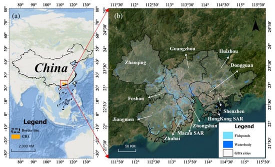
Figure 1.
(a) Geographical location of the GBA in China, and (b) distribution of fishponds in the region.
Topographically, the GBA is dominated by low-relief landscapes that consist primarily of plains and low hills. It is bordered by mountainous areas to the east, west, and north, while the central portion features a broad alluvial plain that gradually extends southward into the South China Sea [38]. The Pearl River Delta (PRD), a major alluvial and estuarine zone within the GBA, supports a highly complex hydrological system composed of an interconnected network of rivers, tributaries, lakes, and fishponds [39].
As one of China’s most economically dynamic regions [40], the GBA contributes approximately 11% to the national gross domestic product (GDP) [41]. The region’s favorable climatic conditions and dense river networks have supported a long-standing tradition of aquaculture. Historically rooted in integrated practices such as the “mulberry dike–fishpond” system, the aquaculture sector has undergone substantial transformation in response to rapid economic development and evolving land-use patterns [42]. In recent decades, traditional low-intensity systems have increasingly been replaced by high-density, intensive aquaculture operations with the aim of maximizing production efficiency [43].
2.2. Landsat Data Acquisition and Image Processing
This study employed imagery from the Landsat 8 and Landsat 9 Operational Land Imager (OLI) sensors to retrieve DO concentrations across the GBA. Landsat 8, launched on 11 February 2013, is equipped with the Operational Land Imager (OLI) and the Thermal Infrared Sensor (TIRS), offering a 16-day revisit cycle. It provides spatial resolutions of 30 m for visible, near-infrared (NIR), and shortwave infrared (SWIR) bands, 100 m for thermal infrared bands, and 15 m for the panchromatic band. Landsat 9, launched on 27 September 2021, is equipped with the upgraded OLI-2 and TIRS-2 sensors, which retain the design specifications and performance characteristics of Landsat 8.
Cross-validation analyses have confirmed the radiometric and geometric consistency between Landsat 8 and Landsat 9, thereby ensuring their interoperability and reliability for long-term, large-scale environmental monitoring applications [44]. For this study, Level-1 terrain-corrected images from both Landsat 8 and Landsat 9 were obtained from the United States Geological Survey (USGS) Earth Resources Observation and Science (EROS) Center. To ensure image quality, only scenes with less than 50% cloud cover were selected. A total of 912 valid satellite scenes were acquired and used for subsequent analysis, and a cloud mask operation was subsequently applied to remove clouds and relevant shadows in the images using the Quality Assessment (QA) Band provided with the Landsat Collection 2 Level-1 products. Therefore, although the original scenes might have high cloud cover, the actual satellite products we used were rigorously cloud-free, which greatly reduced the uncertainty introduced by cloud coverage. As illustrated in Figure 2a,b, eight Landsat images can provide full coverage of the GBA.
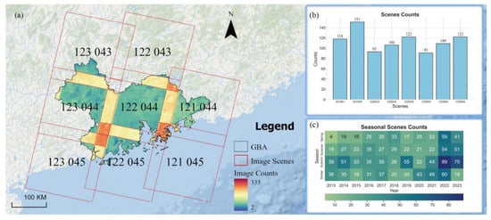
Figure 2.
(a) The spatial distribution and statistics of the availability of Landsat imagery. The orange boxes denote the satellite scenes covering the GBA, with labelled path and row numbers, and the gradient color indicates the number of available images for each pixel. (b) Number of available images for different paths and rows. (c) The seasonal availability of Landsat imagery for different years. Each number represents the quantity of available images for the corresponding season.
In this study, the SeaDAS software was utilized to perform Rayleigh reflectance correction, which allowed the generation of Rayleigh-corrected reflectance products. SeaDAS, developed by The National Aeronautics and Space Administration (NASA), is widely employed in water environment remote sensing applications [45]. It facilitates effective water reflectance correction, ensuring strong spectral consistency between corrected Landsat 8 imagery and in situ spectral measurements [46].
To further mitigate aerosol interference, an additional correction algorithm was applied: R’rc = Rrc (λ) − Rrc (2201). Although this method may not completely remove residual aerosol signals in specific spectral bands, it can effectively reduce atmospheric aerosols, haze, and sun glint artifacts, and thereby improves the accuracy of water reflectance retrieval [47]. The water body boundary was then delineated using the Modified Normalized Difference Water Index (MNDWI) [48] in conjunction with a threshold segmentation method. The MNDWI is a robust technique for surface water extraction, effectively suppressing shadows from mountainous terrain, buildings, and snow cover. Additionally, it demonstrates high performance in detecting small water bodies, such as fishponds, which ensures comprehensive and accurate water body delineation [49]. The corresponding formula is as follows:
where and are the green band and shortwave infrared band of Landsat OLI satellite, respectively.
2.3. Extraction of Fishponds Boundaries and Environmental Variables in the GBA
This study employed fishpond boundary data that were previously delineated in an earlier study conducted by our team [50]. In that study, the preprocessing of satellite imagery covering the GBA involved radiometric calibration, atmospheric correction, and image mosaicking. An object-oriented classification framework was then implemented that involved combining SVM algorithms with manual visual interpretation to achieve high-precision delineation of fishpond boundaries.
The spatial distribution of fishponds revealed a strong association with rivers and coastal zones, with particularly high densities being observed in eastern Zhaoqing, southern Jiangmen, Zhuhai, and ZS. In contrast, the fishpond presence was markedly lower in more urbanized regions such as Guangzhou, HZ, Dongguan, Shenzhen, HK, and Macao. This distributional pattern is closely linked to both regional land-use structures and underlying topographic conditions. In addition to spatial boundaries, this study incorporated environmental data—including TSM [51] and Chl-a concentrations [52]—to examine their influence on DO levels. These datasets provide a foundation for analyzing the spatial heterogeneity and driving mechanisms of DO concentrations in fishponds across the GBA.
2.4. Field Data Collection
To support model training and validation, field-based water quality measurements were conducted at 16 representative fishpond sites across the GBA: five each in FS, HZ, and ZS, and one in HK. Sampling was performed seasonally (spring, summer, autumn, and winter) at each site. In addition, one pond in each of FS, HZ, and ZS was selected for intensive 48 h monitoring, with measurements being collected at two-hour intervals. The remaining ponds in these cities were sampled once per season, while the pond in HK was monitored monthly.
Surface water samples (0–15 cm depth) were collected using a WTW Multi 3320 m to measure key water quality parameters, including WT, DO, electrical conductivity (EC), total dissolved solids (TDS), and salinity. A portable wind speed recorder was used to document meteorological variables such as wind speed (WS), air temperature (AT), and atmospheric pressure (AP) (Figure 3). For Chl-a concentration analysis, water samples were filtered using Whatman GF/F glass fiber filters (25 mm diameter, 0.47 μm pore size), which were then stored at low temperatures and later analyzed in the laboratory using a Turner Designs fluorometer. TSM concentrations were determined by filtering water samples through pre-weighed cellulose acetate membranes (47 mm diameter, 0.7 μm pore size), freezing the filters, and subsequently analyzing them under laboratory conditions.
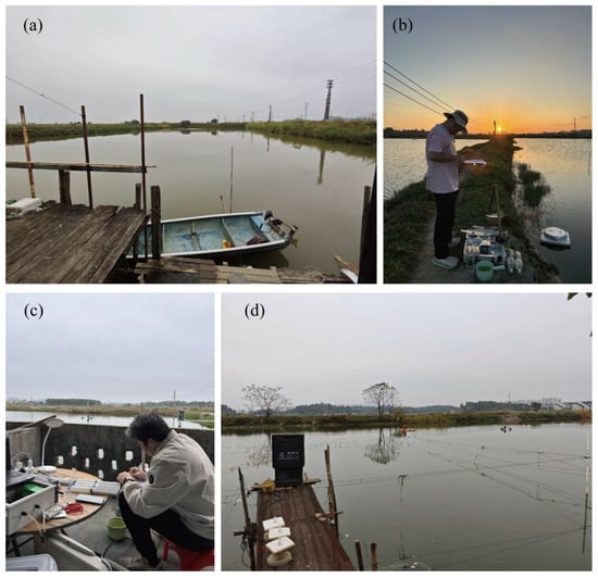
Figure 3.
On-site sampling in fishponds; all the photos were taken by the authors. (a) and (d) are photos of fishponds in Zhongshan and Huizhou, respectively, while (b) and (c) are photos of water samples taken by the author.
The collected field data were used to investigate the environmental drivers of DO variability across different pond systems. Additionally, semi-structured interviews were conducted with local aquaculture practitioners to obtain qualitative insights into farm management practices. The information that was gathered included aquaculture cycles, aeration system usage frequency, and stocking densities—all of which are known to influence DO dynamics in intensive aquaculture environments.
The availability of satellite imagery in the study region is frequently constrained by persistent cloud cover, a defining characteristic of the humid subtropical climate prevailing throughout the GBA. This atmospheric limitation often leads to a lack of temporally coincident satellite observations for many field sampling events, and thereby reduces the number of valid satellite–in situ data pairs available for model development.
To enable an independent and rigorous evaluation of the model’s generalization capability within aquaculture environments, dedicated field sampling campaigns were conducted. In situ observations were temporally matched with Landsat 8/9 imagery using a ±1 day window relative to the satellite overpass. Following a cloud-screening procedure, a final set of 24 high-quality satellite–in situ matchups was obtained. This dataset was strictly reserved for independent validation purposes and was not involved in any phase of model training or parameter optimization. It was used exclusively to assess the predictive accuracy of the final model under real-world fishpond conditions.
To further enhance the representativeness and robustness of the training dataset—particularly at the lower and higher ends of the DO concentration range—additional field measurements were incorporated from adjacent coastal waters. High-DO samples were obtained from official records published by the Guangdong Provincial Department of Ecology and Environment. The initial dataset consisted of 1962 monitoring records. These records were subjected to a two-step filtering process: (1) temporal alignment within ±1 day of a Landsat overpass, and (2) spatial verification to ensure that sampling points were located within cloud-free pixels. This filtering process resulted in a final training dataset comprising 64 valid satellite–in situ matchups from coastal waters.
As presented in Table 1, the observed DO concentrations in this study range from 5.68 to 9.97 mg/L. This relatively short range introduces a potential risk of extrapolation errors when predicting higher DO concentrations (e.g., DO > 10 mg/L) that are outside the original data distribution. Given the absence of a well-established theoretical framework for the underlying natural processes, such extrapolations can be highly uncertain and prone to significant inaccuracies. To mitigate this issue, we included additional DO data from Lake Huron [22], which exhibits a broader DO range (5.84 to 14.77 mg/L), and thereby extended the model’s predictive capacity to higher DO concentrations.

Table 1.
The statistical indicators of in situ DO concentration.
Prior to integrating the Lake Huron data into our model, we conducted a comparative analysis to assess the consistency between the environmental conditions of Lake Huron and those of the aquaculture fishponds included in our study. This analysis revealed a high degree of similarity in key environmental indicators, providing confidence that the Lake Huron data would be contextually appropriate for enhancing the model’s robustness and minimizing the risks associated with extrapolation. Thus, an additional 10 high-DO samples from Lake Huron were incorporated [22], which resulted in a final training dataset consisting of 74 samples from 24 valid images. The spatial distribution of the water quality monitoring sites used for model training is depicted by the red dots in Figure 4a, which represents the sampling locations within the coastal waters of Guangdong Province.
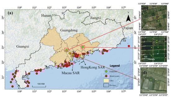
Figure 4.
Spatial configuration of sampling sites: (a) The location of sampling sites in Guangdong province, the green points represent field measurements from fishponds by the authors and red points represent water quality monitoring stations from coastal waters. (b–d) Enlargements of field measurements from fishponds in FS, HZ, and ZS, respectively.
2.5. Empirical Mode Decomposition (EMD)
The weak spectral response of DO concentration variations poses a significant challenge for conventional feature extraction methods, as they often fail to identify spectral features that exhibit strong correlation with DO fluctuations [53]. To overcome this limitation, this study employed the EMD method to extract and analyze multispectral reflectance data (Figure 5). Compared with traditional decomposition techniques (such as wavelet transform or Fourier transform), we emphasize that EMD is more suitable for processing the nonlinear and non-stationary signals commonly seen in remote sensing [54]. Other feature extraction methods, such as principal component analysis (PCA), focus on global variance and pre-set spectral indices for specific relationships. EMD can adaptively decompose spectral signals into intrinsic modes and separate very weak spectral signals or local spectral features related to DO concentrations. If other methods are used, these features may be treated as noise or ignored in the dimensionality reduction process [55].
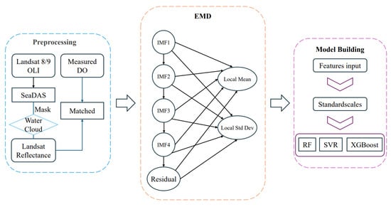
Figure 5.
The flowchart of DO estimation using Landsat data and EMD.
The methodological framework consists of several key steps. First, reflectance data from seven Landsat OLI satellite bands (443 nm, 482 nm, 561 nm, 655 nm, 865 nm, 1609 nm, and 2201 nm) were preprocessed, including atmospheric correction, water body extraction, and cloud masking. Subsequently, EMD was applied to decompose the reflectance values for each pixel. This process involves identifying local extrema within the signal sequence, constructing upper and lower envelopes using linear interpolation, computing the mean of these envelopes, and extracting IMFs from the original signal. The decomposition continues iteratively until the stopping criteria are satisfied [56]. Following decomposition, the energy contribution of each IMF component was calculated to assess its significance. A 3 × 3 moving window was then used to extract local statistical characteristics of IMFs, while a feature validity check was implemented to ensure the presence of at least five non-zero pixels within the window. Additionally, residual components were analyzed to further refine the extracted features. Finally, the extracted features from all bands were combined into a unified feature matrix, normalized, and prepared for subsequent model development. This method enables the effective characterization of multispectral reflectance data through adaptive decomposition and multi-dimensional feature extraction, and thereby improves the accuracy and robustness of DO concentration predictions.
2.6. DO Retrieval Using Machine Learning Method
A RF machine learning model was developed to estimate the DO concentrations in fishponds across the GBA. A RF model is an ensemble-based algorithm that constructs a robust predictor by bootstrapping multiple decision trees and aggregating predictions through voting (for classification) or averaging (for regression) [57,58]. Unlike other powerful ensemble methods such as XGBoost, RF demonstrates reduced sensitivity to hyperparameter tuning and greater resistance to model overfitting, which is particularly beneficial when working with environmental datasets that are often characterized by inherent noise and variability. This robustness reduces the risk of overfitting, ensuring more reliable generalization when the model is applied to complex ecological data. Secondly, RF models are inherently more resilient to multicollinearity among input features, a common issue in environmental datasets where many variables are interrelated. This capability allows RF models to effectively utilize correlated spectral features without a significant degradation in model performance. Additionally, the RF method is well-suited to capturing non-linear relationships between spectral data and water quality parameters, which makes it an excellent choice for modeling the often complex and non-linear interactions that govern DO dynamics. Our decision to use a RF model was further supported by this method’s successful application in several previous studies specifically focused on DO estimation [20,27]. These studies demonstrated RF’s effectiveness in similar contexts, providing additional confidence in its suitability for this task. Taken together, these practical advantages—including robustness to noise, ease of parameter tuning, effective handling of collinearity, and strong performance with non-linear relationships—along with its established track record in related research, made RF the most appropriate primary ensemble learning model for this study.
A total of 74 matched data sites were randomly divided into a training set (n = 51) and a testing set (n = 23). The RF model used features extracted from EMD as inputs, including four IMFs, one residual component, and their corresponding local mean and local standard deviation values. The model’s robustness and overfitting prevention were achieved by tuning key hyperparameters, such as the number of decision trees, the maximum tree depth, and the number of features considered at each split. To optimize these parameters, Python’s GridSearch was implemented with five-fold cross-validation, which resulted in an optimal ensemble of 200 trees, a maximum tree depth of 10, and other fine-tuned parameter settings (Table 2).
Table 2.
Hyperparameters for each regression model.
The preprocessing of reflectance data for model training involved an initial atmospheric correction using the SeaDAS software, which was followed by a supplementary aerosol interference reduction based on the method proposed by Feng et al. [47]. This approach involved subtracting the reflectance of the SWIR2 band from the first six OLI bands to further minimize aerosol contamination. Following these correction procedures, all input features were standardized using z-score normalization to ensure consistent scaling across variables. This standardization step is critical for enhancing model stability and promoting faster convergence during the training process, as it mitigates the impact of feature scale disparities. As a result of this comprehensive preprocessing and optimization process, a robust RF model was developed that is capable of accurately retrieving DO concentrations from fishponds in the GBA. This model provides a reliable technical foundation for future water quality monitoring and environmental management applications, supporting more precise and data-driven decision-making.
To further assess the performance of the proposed RF model, two alternative machine learning models—SVR and XGBoost—were developed and directly compared. The SVR model utilized kernel functions to project EMD-decomposed features into a high-dimensional space, which allowed it to capture complex, nonlinear relationships within the dataset more effectively [59]. In contrast, the XGBoost model employed a gradient boosting framework that iteratively minimizes prediction errors by combining the outputs of multiple weak learners, which thereby enhances the overall model accuracy and robustness [60]. Both SVR and XGBoost models have been widely adopted in water quality assessment studies, including the estimation of DO concentrations [9,61,62].
To ensure a consistent and unbiased comparison, the SVR and XGBoost models were trained using the same set of input variables and training datasets as the RF model. All models were implemented in Python 3.11 using the scikit-learn (version 1.6.1) and XGBoost (version 2.1.4) libraries. Data preprocessing, including feature scaling and decomposition, as well as model evaluation, was conducted within the scikit-learn framework. Additionally, GridSearchCV was employed for hyperparameter tuning to optimize each model’s performance and ensure that the final models reflect their maximum predictive potential.
2.7. Model Validation
To evaluate the accuracy of the developed models, three statistical metrics were employed: the coefficient of determination (R2), root mean square error (RMSE), and mean absolute percentage error (MAPE). The R2 represents the proportion of variance in the dependent variable that can be explained by the independent variables, with higher values indicating superior model performance. The RMSE quantifies the average magnitude of prediction errors, with lower values signifying a more accurate model. Meanwhile, the MAPE expresses the average absolute error as a percentage of the actual values, with lower percentages corresponding to more precise predictions. The mathematical formulas for these three metrics are as follows:
where represents the predicted value of DO, represents the measured value of DO, is the mean value of the observations, and is the number of sampling records.
2.8. Spatial Patterns and Spatiotemporal Characteristics of Dissolved Oxygen in Fishponds
Sen’s slope is a non-parametric statistical method used for trend assessment. In a time series, the trend is measured using the β value, where β > 0 indicates an increasing trend, while β < 0 signifies a decreasing trend. The Mann-Kendall (MK) trend test, a widely used non-parametric method in climate and hydrological studies, evaluates the statistical significance of a trend by computing the Z score. When the absolute value of Z exceeds or equals 1.64, 1.96, and 2.58, the trend is considered statistically significant at confidence levels of 90%, 95%, and 99%, respectively. Both trend analysis methods were implemented using the Mann-Kendall Python package. The formulas are as follows:
where is the number of samples and indicates whether the difference between the measurements at time and are positive, negative or zero. is the difference between the number of positive differences and the number of negative differences. is used to calculate the variance, is the number of tie groups in the data, is the number of records contained in the -th tie group, and ensures large sample sizes.
2.9. Lindeman, Merenda, and Gold (LMG)
The LMG model quantifies the contribution of each independent variable by incrementally decomposing R2 in a multiple linear regression. This approach is independent of the order of predictor variables, effectively mitigating the hierarchical effect among regression factors. As a result, it provides an unbiased assessment of the relative contributions of explanatory variables to the DO concentration. Due to its robustness, the LMG model has been widely applied in ecological and environmental studies [63,64]. The mathematical formulation for the LMG model is presented in Equation (10).
In the formula, represents the sequence; ; is the order in which the variable was inputted to the model; represents the combination of variables before , which are added to the model in the th arrangement; represents the average increment in caused by the input of . This study used WT, pH, WS, EC, salinity, AP, nitrate, nitrite, ammoniacal nitrogen (AN), TSM, and Chl-a as explanatory variables. The LMG model was constructed using R language (version 4.4.0) to obtain the relative contribution of each factor to DO fluctuations. However, in some fishponds, the salinity, EC, and TDS have strong linear relationships, so only EC is used as an explanatory variable.
3. Results
3.1. Model Performance and Limitations
This study evaluated the performance of three widely used machine learning models in the spectral estimation of DO concentrations in aquaculture systems (Figure 6). The results demonstrate that all three models exhibit strong predictive capability when applied to spectral data decomposed via EMD. Among them, the RF model achieved the highest accuracy, with an R2 of 0.8249, RMSE of 0.4386 mg/L, and MAPE of 3.13%. However, due to an insufficient input of high-DO-concentration samples in the training dataset, all models tended to underestimate high DO values, with the RF model displaying the least bias. Additionally, a slight overestimation tendency was observed across the models when predicting low DO concentrations.
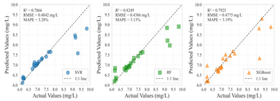
Figure 6.
Accuracy comparison with three machine learning models.
To assess the real applicability of the model, a 3 × 3-pixel window was used to extract DO concentrations from the retrieved results, which were then compared with corresponding in situ measurements. The results (Figure 7) indicate that the RF model maintains robust predictive reliability under practical conditions, with an R2 of 0.7050, an RMSE of 0.4218 mg/L, and a MAPE of 4.30%, respectively. These findings suggest that the model demonstrates strong regional adaptability and holds significant practical utility.
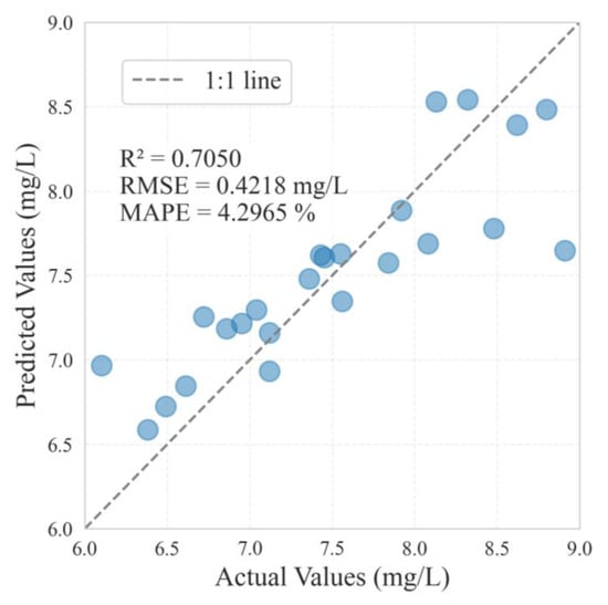
Figure 7.
The assessment of robust predictive reliability of the RF model under practical conditions.
3.2. Spatial Pattern of DO Levels Across the GBA
Figure 8 illustrates the spatial distribution of average DO concentrations in the GBA from 2013 to 2023. In this region, the DO levels predominantly range from 6.80 to 8.45 mg/L, with an overall average of 7.44 mg/L (Table 3). Higher DO concentrations are primarily observed in the central regions of the study area, including Zhaoqing, western FS, northern Jiangmen, and HZ, while lower levels are evident in peripheral regions such as southern Jiangmen, southern Guangzhou, ZS, and eastern FS. Overall, there is a clear trend of decreasing DO levels from the periphery toward the center of the region. Moreover, significant human interventions can cause areas with similar natural conditions to exhibit varying DO concentrations.
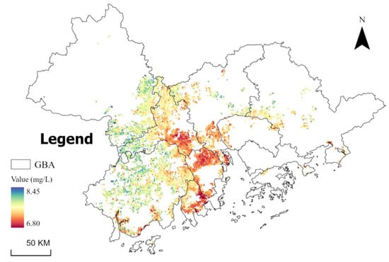
Figure 8.
The spatial distribution of DO concentrations across the GBA.
Table 3.
The statistical indicator of results for the mean annual DO concentration.
3.3. Interannual and Seasonal Variations in DO Concentrations
An analysis of the predicted DO concentrations from 2013 to 2023 (Figure 9 and Figure 10) revealed that, although the annual mean DO concentrations exhibited fluctuations, they remained relatively stable overall, with no obvious trend. Specifically, during the 2013–2014 period, the DO concentrations experienced a slight upward trend, increasing by 1.6%. In the subsequent period (2014–2016), the DO levels experienced a continuous decline, with a cumulative decrease of 2.2%. Between 2016 and 2018, the DO concentrations changed more markedly, initially increasing by 2.7%, followed by a 1.3% decline, which indicates a slight oscillatory behavior. From 2019 to 2023, the DO concentrations entered a relatively stable phase, with only minor fluctuations being observed, which suggests a gradual stabilization of water quality dynamics in the study area.
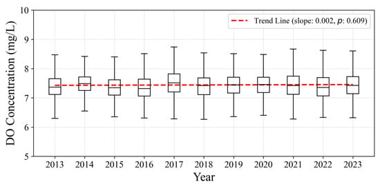
Figure 9.
The annual changes in DO concentrations in the GBA from 2013 to 2023.
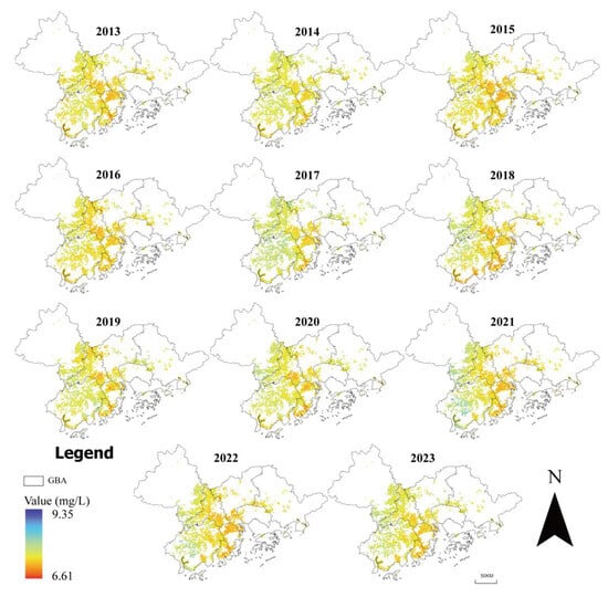
Figure 10.
The spatial distribution of annual DO concentrations across the GBA from 2013 to 2023.
In addition, this study revealed distinct seasonal patterns in the DO concentrations within fishponds. The results (Figure 11) demonstrated that the mean DO levels reached their maximum in summer (7.5 mg/L) and their minimum in winter (7.16 mg/L), exhibiting a pattern that contrasts with the seasonal variations observed in natural water bodies. Spatially, the western GBA region, encompassing Zhaoqing, Jiangmen, and western FS, showed notably higher DO concentrations during spring and autumn compared to the eastern region (Figure 12). Interestingly, the fishponds in Zhuhai and ZS consistently maintained lower DO concentrations throughout all seasons. Natural water bodies, on the other hand, display more pronounced seasonal characteristics. Figure 11 also shows the variation in the DO in rivers, which is distinct from that of the fishponds. Originally, the DO in winter is higher than that in other seasons and reaches the lowest concentration in summer.
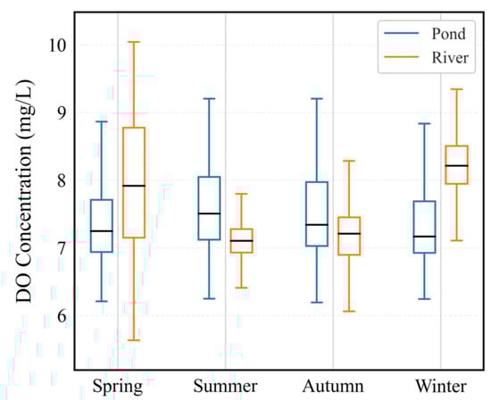
Figure 11.
Box plot of the seasonal ranges of DO concentrations in fishponds and rivers in the GBA from 2013 to 2023. The black line indicates the median concentration.
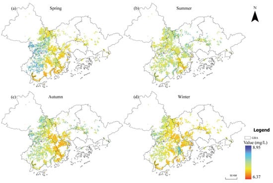
Figure 12.
The seasonal patterns of the mean DO concentrations in fishponds in the GBA from 2013 to 2023. (a), (b), (c) and (d) represent spring, summer, autumn, and winter, respectively.
3.4. The Long-Term Variation of DO Concentration in GBA
To further analyze the trends in the DO concentrations in fishponds within the GBA, this study applied the MK trend test across different regions. The GBA was divided into 10 administrative regions—Dongguan, FS, Guangzhou, HK, HZ, Jiangmen, Shenzhen, Zhaoqing, ZS, and Zhuhai, with Macau SAR being excluded due to the limited presence of fishponds. The average Z values were below 1.69, indicating that the DO concentration changes were not statistically significant across these areas.
However, as shown in Figure 13, some fishponds exhibited distinct upward trends in their DO concentrations, particularly in eastern Jiangmen and Zhaoqing. In contrast, the ponds with significant downward trends were sporadically distributed across various regions without apparent clustering. Although the MK test (Figure 13a) did not indicate a statistically significant overall trend, Sen’s slope analysis (Figure 12b) revealed a gradual increase in DO concentrations from 2013 to 2023 (β = 0.08). Only Zhaoqing exhibited a negative mean β value among the 10 regions, whereas all other regions showed positive values, with Shenzhen recording the highest (β = 0.239). Most regions experienced a slow increase in their DO concentrations, with only a few areas showing minor declines. While the DO concentrations in the GBA have gradually increased over the past decade, this trend remains statistically insignificant.
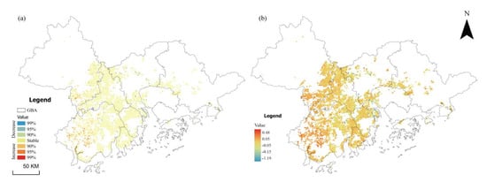
Figure 13.
Trend tests for the long-term DO variation in the GBA during 2013–2023. (a,b) The results of the M-K test and Sen’s slope test for DO concentration variations with Z-values and β-values sampled at 0.01° × 0.01° intervals.
4. Discussion
4.1. The Impact Factors of DO Concentration Changes
Numerous studies have examined the factors that influence DO concentrations, primarily focusing on natural environments such as oceans, rivers, and lakes [8,22,65]. However, relatively few have examined DO dynamics in fishponds, which are strongly disturbed by human activities. Utilizing measured data from both fishponds and a coastal river in Guangdong [66], this study analyzed and evaluated the key drivers of DO concentration changes in fishponds and compared them with those in natural water bodies. Furthermore, the relationships between the DO levels and explanatory variables were elucidated through correlation analysis, while the LMG model was employed to quantify the relative contributions of these variables, providing critical insights to support the model’s predictions.
As shown in Figure 14, the DO concentration exhibited the strongest correlation with the pH across four studied fishponds, whereas associations with other variables were less pronounced. Specifically, for the all-year data, the correlation coefficients between the DO and pH in the measured samples were 0.55, 0.62, 0.84, and 0.75 (p < 0.05), respectively, with the pH emerging as the most influential predictor in the LMG model. Furthermore, the pH exhibited a consistently strong positive correlation with the DO levels, both within diurnal cycles and across seasonal variations, with typical correlation coefficients exceeding 0.7 and statistical significance at the p < 0.05 level. When considering the entire dataset, the overall correlation coefficient reached 0.79 (p < 0.001), indicating a robust association. Notably, the relative contribution of the pH to the observed DO variability was approximately 70% (Figure 15), which underscores its critical role in regulating oxygen dynamics within the study area. These findings suggest that the pH serves as a key indicator of DO fluctuations in these aquatic environments. Previous studies have highlighted the critical role of the pH in DO prediction models for natural water bodies [67,68]. The strong correlation between the pH and DO is primarily driven by carbonate equilibrium and biological processes such as photosynthesis and respiration mechanisms that have been widely observed across various aquaculture settings [69,70]. In fishponds, daytime algal photosynthesis significantly reduces dissolved carbon dioxide (CO2) concentrations, leading to an increase in pH levels due to the limited dissociation of bicarbonate ions (HCO3−) required to replenish CO2 [71]. This process is further amplified under high light intensity, as photosynthesis generates substantial amounts of oxygen, which results in pronounced increases in DO concentrations. Conversely, during nighttime hours, respiration by aquatic organisms and the microbial decomposition of organic matter in sediments release CO2 while simultaneously consuming oxygen. This leads to a concurrent decline in both the DO and pH levels as the biological demand for oxygen surpasses its production [72]. This study empirically confirmed the strong positive correlation between DO and pH using field measurements from fishponds in FS, HK, HZ, and ZS, further reinforcing the critical role of pH as a key driver of DO variability in managed aquaculture systems.
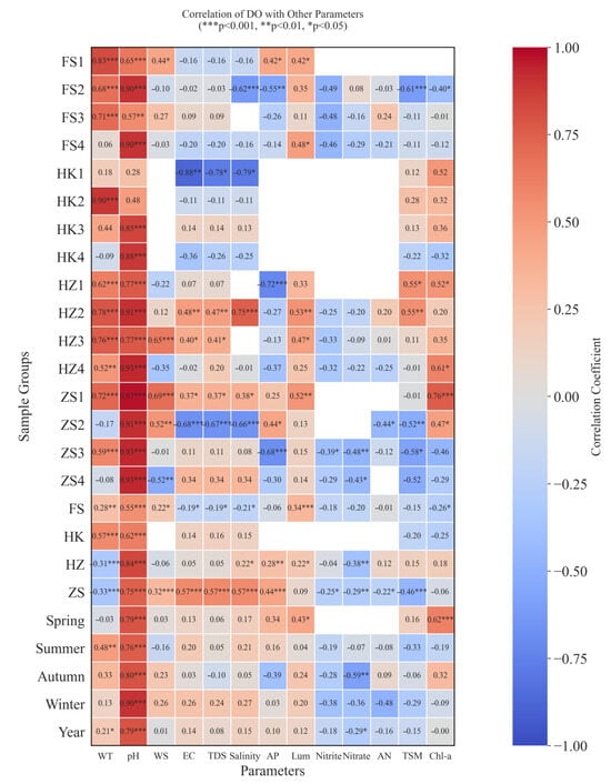
Figure 14.
Correlation coefficients between DO concentrations and other factors in fishponds. The parameters include water temperature, pH, wind speed, electrical conductivity, total dissolved solids, salinity, atmospheric pressure, light intensity, nitrate, nitrite, ammoniacal nitrogen, total suspended matter, and chlorophyll-a.
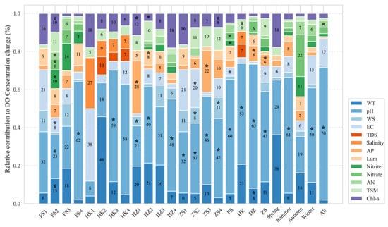
Figure 15.
Relative contribution of environmental drivers to DO variability in fishponds across different regions (FS, HK, HZ, ZS) and seasons, as determined by the LMG model (* p ≤ 0.05). The numerals 1–4 following each group name correspond to seasonal sampling periods from spring to winter, respectively. Environmental variables contributing less than 1% to the total explained variance are not displayed.
WT is widely recognized as a key determinant of DO dynamics, typically exhibiting a strong negative correlation with DO concentrations due to its influence on both oxygen solubility and aquatic metabolic rates [65]. For instance, Topcu et al. [8] reported that the DO concentrations in the North Sea decrease substantially during the summer months, reaching an annual minimum of 6.5 mg/L in August, while remaining elevated during the winter. Similarly, Guo [22] observed seasonal fluctuations in the DO concentrations in Lake Huron (1984–2019), with the values declining to 8.53 mg/L in July and peaking at 12.25 mg/L in November—an overall seasonal range of approximately 4.0 mg/L.
In the coastal river analyzed in this study (Table 4), a strong negative correlation was observed between the WT and DO (r = –0.69, p < 0.05), which is consistent with patterns documented in various natural aquatic systems, including the Yellow Sea of Korea (r = –0.74, p < 0.05) [14], Lake Huron (r = –0.71, p < 0.05) [22], and the Zhejiang coastal waters during summer (r = –0.80, p < 0.05) [13]. Similarly, significant negative correlations were found in fishponds in HZ and ZS, with correlation coefficients of –0.31 and –0.33 being observed, respectively (p < 0.05), which aligns with thermodynamic expectations of reduced oxygen solubility at higher temperatures.
Table 4.
Comparison of WT–DO correlations in different waters.
However, contrasting patterns were identified in the fishponds of FS and HK, where the WT and DO demonstrated significant positive correlations (r = 0.28 and 0.57, respectively; p < 0.05), accounting for 5% and 21% of the variance that was explained. Further analysis revealed that this anomalous relationship persisted across multiple temporal scales. Notably, 9 out of 12 diurnal observation sets revealed a statistically significant positive correlation between the WT and DO. Seasonal stratification of the data showed consistent positive correlations across summer, autumn, and winter, with the strongest relationship being observed during summer (r = 0.48, p < 0.01, 5%). Moreover, when all fishpond data were pooled across the entire year, the overall correlation between the WT and DO remained positive (r = 0.21, p < 0.05, 1%).
This counterintuitive positive correlation is attributed to the unique environmental and management conditions of intensively regulated aquaculture systems. Unlike natural water bodies, where the DO patterns are primarily driven by temperature-dependent solubility and biological demand, the DO levels in managed fishponds are more tightly controlled. Seasonal fluctuations are often attenuated or reversed due to anthropogenic interventions. For example, the observed higher DO levels in summer and lower levels in winter reflect a management-driven seasonal regime that is shaped by high feeding intensity and nutrient loading during the warmer months, which stimulates substantial algal growth and photosynthetic oxygen production [73].
This photosynthetic activity, particularly during daylight hours when satellite observations are typically acquired, can elevate surface DO concentrations and offset the expected solubility-driven DO reductions associated with higher summer temperatures. Consequently, in such environments, the influence of the temperature on DO dynamics is modulated or offset by other factors, including diurnal biological processes, water exchange, and artificial aeration. The anomalous DO–WT relationship observed in these aquaculture systems underscores the complexity of DO dynamics in anthropogenically managed environments. It highlights the need to consider both natural and artificial influences—including metabolic cycles, algal productivity, and management practices—when interpreting DO trends and developing remote sensing-based predictive models for aquaculture applications.
In addition to the WT, environmental variables such as the AP, light intensity, and TSM also exhibited site-specific influences on the DO concentrations across the study area. In ZS, the AP and TSM showed the strongest correlations with the DO, with correlation coefficients of r = 0.44 and r = –0.46, respectively (p < 0.001), contributing approximately 6% and 9% to the total variance in DO levels. By contrast, these variables had a more limited impact in FS and HZ. For instance, in FS, the light intensity was the most influential parameter (r = 0.34, p < 0.001), although its relative contribution remained modest at 7%.
These observed correlations reflect the net influence of each factor over the study periods, yet the mechanisms underlying these relationships often operate on much shorter temporal scales. For example, the positive correlation between the light intensity and DO concentrations is largely attributable to photosynthesis—a process characterized by pronounced diurnal variation (e.g., r = 0.52, p < 0.01 at site ZS1). Similarly, the AP and TSM concentrations can respond rapidly to short-term meteorological events such as heavy rainfall, which may simultaneously enhance the DO through atmospheric reaeration (often associated with reduced AP and increased turbulence) and reduce it through increased TSM loads that limit light penetration or promote the decomposition of suspended organic matter.
Despite the statistical significance of certain variables during specific time periods (e.g., springtime light intensity, r = 0.43, p < 0.05, contributing approximately 3%), their explanatory power for long-term DO variability remains limited. Across most sites and seasons, the relative contributions of the AP, light intensity, and TSM were generally low, typically below 1% (e.g., 0.5% for AP, 0.4% for light intensity, and 1% for TSM). Even the highest observed contribution of 9% for the TSM in ZS suggests that, while these variables can exert meaningful short-term effects, they are unlikely to serve as primary drivers of broader seasonal or interannual DO patterns.
Salinity, along with its closely related proxies—EC and TDS—also played a measurable role in modulating DO concentrations through their influence on oxygen solubility and associated biogeochemical processes. Correlation analysis (Figure 14) revealed high collinearity among the EC, TDS, and salinity, as evidenced by their similar trends with DO across the sampling groups. Notably, these relationships were highly site-specific. In ZS, for example, all three variables exhibited significant positive correlations with DO (e.g., salinity: r = 0.57, p < 0.001). This finding is somewhat counterintuitive, as elevated salinity typically reduces the oxygen solubility due to increased ionic strength. Similar, although generally weaker, positive associations were also observed in certain HZ samples, which indicates that this phenomenon may not be isolated to ZS.
Conversely, in FS and HK, the correlations between salinity-related variables and the DO were weak or non-significant. The pronounced spatial heterogeneity of these correlations—particularly the anomalous positive trends in ZS—suggests that local environmental or management factors may be mediating these effects. Potential contributors include site-specific aquaculture practices, differential water exchange rates, and variations in organic and nutrient inputs. These findings highlight the need for site-specific investigations to disentangle the physical and biogeochemical mechanisms influencing the variability in DO.
Due to the strong collinearity among the EC, TDS, and salinity, their individual effects could not be effectively separated within the LMG model. Therefore, the EC was retained as a representative variable to reduce redundancy and minimize multicollinearity. Model outputs indicated that the EC had a limited influence on the variability in DO across all four sites, with its highest relative contribution being observed in ZS (9%). This suggests that, although the EC may affect the DO under certain conditions, its role in driving cyclical or seasonal DO variation is minimal, likely due to its relative stability throughout the aquaculture cycle.
Interestingly, in the coastal river system (Figure 16), the correlation between the EC and DO was substantially stronger (r = 0.71, p < 0.05), indicating that EC fluctuations play a more prominent role in shaping the DO dynamics in hydrologically active environments. This disparity may stem from the higher hydrodynamic variability in open river systems, where changes in EC more directly affect oxygen solubility and vertical mixing processes.
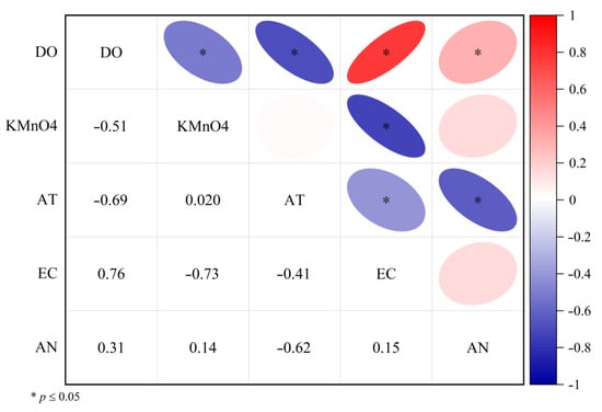
Figure 16.
Correlation between DO concentrations and other factors in the coastal river. The key parameters include permanganate index, air temperature, pH, electrical conductivity, and ammoniacal nitrogen.
The nutrient levels also displayed complex and site-dependent relationships with the DO concentrations, underscoring the context-specific nature of nutrient–oxygen interactions. While the eutrophication pathway—where excess nutrients promote algal blooms followed by oxygen depletion through microbial respiration—is well-established [74], this mechanism was not uniformly reflected in the correlation patterns across all sites. Significant negative correlations were observed in the overall datasets for HZ (nitrate: r = –0.38, p < 0.01, 6%) and ZS (nitrate: r = –0.29, p < 0.05, 4%), which suggests that nutrient-driven oxygen depletion processes were active in these regions. However, this relationship was less apparent in FS, where the influence of nutrients may have been moderated or masked by factors such as increased water circulation or aeration.
These findings highlight the indirect and often nonlinear nature of the effects of nutrients on the DO, which are mediated through biological processes including algal productivity, respiration, and organic matter decomposition. The role of Chl-a, a widely used proxy for phytoplankton biomass, further exemplifies these complex interactions. Heatmap analysis revealed significant positive correlations between the Chl-a and DO at specific sites and time periods (e.g., HZ1: r = 0.52, p < 0.05, 12%; spring: r = 0.62, p < 0.001, 17%), which likely reflects the dominance of photosynthetic oxygen production under favorable light conditions, particularly given the high baseline Chl-a levels observed in the region [52].
However, this positive relationship was not consistently observed. In the overall ZS dataset, the correlation between the Chl-a and DO was weak and non-significant (r = –0.06, p > 0.05), which suggests that the oxygen production through photosynthesis may have been counterbalanced by the respiration or decomposition of algal biomass, especially during nighttime or in eutrophic conditions (Figure 17). These findings reinforce the notion that the DO dynamics in aquaculture environments result from a multifaceted interplay of physical, chemical, and biological processes—many of which are further shaped by human management practices.
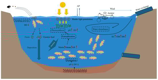
Figure 17.
Schematic diagram of factors influencing DO in fishponds. The parameters include dissolved oxygen, pH, wind speed, electrical conductivity, total dissolved solids, salinity, atmospheric pressure, nitrate, nitrite, and ammoniacal nitrogen. Upward arrows indicate an increase in concentration, while downward arrows indicate a decrease.
Additionally, the strength and direction of the relationship between the Chl-a and DO varied considerably across temporal scales. While a strong positive correlation was observed during the spring sampling period, this relationship weakened or became statistically non-significant in other seasons—for example, in autumn (r = 0.24, p > 0.05, 1.6%), winter (r = 0.20, p > 0.05, 3.4%), and when considering the entire annual dataset (r = –0.00, p > 0.05, 2.4%). These results suggest that the Chl-a–DO relationship in aquaculture systems is highly context-dependent, being influenced by seasonal dynamics, site-specific conditions, and the prevailing biogeochemical environment. This variability is likely driven by the dual functional role of algae in aquatic ecosystems: while algae contribute to oxygen enrichment through daytime photosynthesis, they also consume oxygen via respiration and the microbial decomposition of algal biomass, particularly under conditions of organic overloading. These opposing processes can result in dynamic, and at times contradictory, influences on net DO concentrations.
Such complexity is especially pronounced in eutrophic systems, where algal-driven oxygen fluctuations tend to be both intense and unpredictable [73]. Based on the preceding analyses, the factors influencing the DO concentrations in fishponds exhibit both similarities and clear deviations from the patterns observed in natural water bodies. Among all environmental variables that were assessed, the pH exhibited the strongest and most consistent positive correlation with the DO, a finding that is in line with previous studies. However, the relationship between the temperature and DO demonstrated unexpected regional heterogeneity, including instances of positive correlations that deviate from classical thermodynamic expectations. This anomaly underscores the influence of site-specific aquaculture practices and artificial regulation on DO dynamics.
Similar to temperature, other environmental variables—including the AP, light intensity, and TSM—exhibited highly localized effects. In contrast, the influence of the EC, TDS, and salinity was more strongly associated with the method and frequency of water exchange, as discussed in the section on artificial interventions. The observed negative correlations between nutrient concentrations and the DO further emphasize the critical role of feed management and nutrient control in maintaining water quality. Excessive nutrient loading can exacerbate oxygen depletion through eutrophication and subsequent microbial oxygen consumption. Conversely, the seemingly paradoxical nature of the Chl-a–DO relationship highlights the intricate and often nonlinear interplay between the biotic and abiotic processes that regulate DO concentrations in intensively managed aquaculture systems.
Collectively, these findings advance our understanding of the complex dynamics governing the DO variability in fishponds and underscore the significant influence of artificial management practices. They also highlight the limitations of applying conventional ecological models derived from natural systems to managed aquatic environments without adjustment for anthropogenic factors. Future research should prioritize the integration of high-resolution spatiotemporal monitoring with process-based modeling frameworks. Such approaches are essential for disentangling the multifactorial interactions between environmental variables and management interventions, improving the predictability and sustainability of DO regulation in aquaculture ecosystems.
4.2. Analysis of Human Activity Intervention Intensity
The DO dynamics in fishponds are predominantly governed by anthropogenic management practices rather than natural environmental processes. Farmers tailor management strategies to the physiological requirements of specific cultured species. For example, in the sampled ponds of FS, largemouth bass (Micropterus salmoides), a species that is highly sensitive to the temperature and quality of water [74], necessitate stringent environmental controls. To accommodate these demands, farmers implement precise aquaculture interventions, such as regular water replenishment to buffer against thermal variability [75] and the application of microbial regulators to maintain a stable microbial ecosystem [76].
During the primary growth period of largemouth bass (May–October), their metabolic activity and feeding intensity increase markedly [77], which results in elevated oxygen consumption and subsequent DO depletion [78]. In contrast, the aquaculture strategies in HK diverge significantly between fish and shrimp production systems. Shrimp species generally exhibit a wider tolerance to ammonia-nitrogen concentrations and phytoplankton density [79]. To stabilize ammonia levels, farmers frequently apply water quality enhancers, which inadvertently promote phytoplankton proliferation. Enhanced photosynthetic activity in these systems leads to increased DO production, often resulting in higher DO concentrations in shrimp ponds relative to those used for fish culture [73].
Water exchange mechanisms further contribute to spatial variations in DO dynamics. In ZS, for example, the proximity to a sea inlet enables the use of a tidal water exchange system. This natural exchange mechanism, driven by tidal fluxes, provides the frequent and continuous replenishment of oxygen-rich seawater, ensuring superior water quality conditions. As a result, the DO concentrations in the ZS ponds showed significant correlations with the EC, TDS, salinity, and TSM levels. Similarly, in the adjacent coastal river, the DO was highly correlated with the EC, which reflects the hydrodynamic influence of this variable on the solubility and distribution of DO. Compared to regions that are dependent on artificial water exchange, the efficient tidal renewal system in ZS supports consistently higher DO levels, which emphasizes the critical role of natural water exchange processes in sustaining optimal aquatic health.
Land-use patterns serve as indicators of anthropogenic interventions in aquaculture systems. To assess its influence of these patterns on the quality of water, this study utilized 30 m resolution land-use data [80] to categorize the variations in three key water quality parameters across fishponds (Table 5). Significant differences in water quality metrics were observed among fishponds with different land uses in the GBA. The average DO concentration across the GBA fishponds was 7.44 mg/L. However, the ponds located within built-up areas exhibited significantly lower DO levels, likely due to the economic pressures associated with high land costs, which incentivize high-density aquaculture practices. This intensified stocking density amplifies the oxygen demand, leading to greater DO depletion.
Table 5.
Comparison of major water quality parameters in fishponds with different land uses.
In contrast, the fishponds situated in agricultural landscapes exhibited slightly elevated DO concentrations, while the highest DO levels were recorded in ponds surrounded by forests. This trend aligns with patterns observed in natural water bodies, as inland waters in both agricultural and built-up areas experience water quality degradation due to anthropogenic pollutants, which reduces their DO availability [81,82].
The TSM concentrations followed a spatial distribution pattern that was similar to that of the DO variability. The fishponds in built-up areas recorded the highest TSM concentrations, averaging 62.12 mg/L, a phenomenon likely driven by frequent substrate disturbances, increased organic waste accumulation, and high-density farming activities. In contrast, the lowest TSM concentrations (22.41 mg/L) were found in ponds within forested areas, where minimal anthropogenic disturbance resulted in reduced particulate matter loads.
Unlike the DO and TSM, the Chl-a concentrations displayed relatively uniform distributions across different land uses, consistently ranging between 53 and 54 μg/L. This suggests that, while land-use-driven anthropogenic inputs strongly influence DO and TSM variability, the Chl-a concentrations remain relatively stable across different aquaculture settings. These findings underscore the differential impacts of aquaculture intensity on the quality of water.
High-density aquaculture operations in urbanized areas significantly lower DO levels while increasing TSM accumulation, whereas ponds situated within forested and agricultural areas, experiencing reduced anthropogenic pressures as a result, generally exhibit better water quality conditions. This spatial distribution highlights the potential risks associated with excessive human intervention, which may disrupt the DO balance in aquaculture systems.
Therefore, in balancing economic viability with environmental sustainability, aquaculture strategies should prioritize optimized stocking densities to maintain DO homeostasis and enhance the overall water quality. Future research should integrate remote sensing techniques, machine learning models, and in situ monitoring to develop adaptive aquaculture management frameworks that ensure ecological resilience while maximizing production efficiency.
4.3. Limitations and Future Work
While this study presents a robust framework for remotely sensing DO concentrations in fishponds, it is important to acknowledge several technical limitations and sources of uncertainty inherent to the methodology.
A primary constraint lies in the spatial resolution of the Landsat imagery that was employed, which is limited to 30 × 30 m. Given the relatively small and often irregular geometry of fishponds, particularly along their narrow perimeters, this spatial resolution may result in mixed-pixel effects. These effects can introduce localized inaccuracies by combining spectral signals from adjacent land or water features. To assess the potential impact of these uncertainties on regional-scale findings, we conducted a temporal stability analysis using a time series of over 110 million pixels. The assumption was that noise induced by mixed pixels would likely manifest as unstable or spurious trends over time. The results indicated that only 0.38% of the analyzed pixels exhibited statistically significant trends, while over 99.6% remained stable. This suggests that, although pixel-level inaccuracies due to mixed-pixel effects may exist, their influence was minimal and did not substantially compromise the integrity of the broader spatiotemporal patterns identified in this study.
A second limitation stems from the temporal mismatch between the satellite revisit times and in situ field sampling. DO exhibits pronounced diurnal variability, which is influenced by photosynthesis, respiration, and management activities such as aeration. Although a ±1-day window was employed to match the field observations with Landsat revisit dates, this temporal gap inevitably introduces possible uncertainties. As such, the current validation approach may not fully capture the instantaneous DO conditions at the time of satellite imaging, which could affect the model’s precision.
To address these limitations and improve prediction accuracy, several potential avenues for future research can be considered: (1) The incorporation of deep learning algorithms: Advanced deep learning models could be employed as inversion tools to capture the complex, non-linear relationships between spectral data and water quality parameters. These methods have demonstrated significant potential for improving inversion accuracy by effectively learning the intricate spectral signatures associated with DO concentrations. (2) The utilization of higher spatial resolution data: To overcome the challenges associated with the relatively small size of many fishponds, satellite data with higher spatial resolution should be explored. For example, Sentinel-2 imagery, which offers a 10–20 m spatial resolution for relevant spectral bands, has already been successfully applied in dissolved oxygen inversion studies. The use of such higher-resolution data would enable the more precise delineation of individual ponds and thereby reduce the impact of mixed-pixel effects and enhance the overall model performance. (3) Enhanced synchronous data collection: The most effective strategy for minimizing uncertainties arising from temporal mismatches is the implementation of field campaigns that synchronize in situ water quality measurements with satellite revisits. Coordinated monitoring efforts would enable more precise model training and validation, and thereby improve the reliability and interpretability of remote sensing-based assessments.
By integrating these advancements, future studies can build on the current findings to achieve more precise and reliable monitoring of the DO dynamics in complex aquaculture landscapes, which would ultimately support more effective environmental management and decision-making.
5. Conclusions
This study investigated the spatiotemporal dynamics of the DO concentrations in fishponds across the GBA for the period 2013–2023, revealing that anthropogenic management practices play a dominant role over natural environmental factors in regulating DO levels. Key influencing factors include the water exchange mechanisms, aeration, stocking density, and nutrient management, with the temperature, AP, light intensity, and TSM contributing to regional variations. Significant spatial heterogeneity in the DO levels was observed, with higher concentrations being observed in shrimp ponds and tidal-exchange systems (e.g., Zhongshan) and lower concentrations being observed in high-density aquaculture within urbanized areas, where elevated stocking densities and organic waste accumulation drive DO depletion. Nutrient loading was identified as a key driver of DO depletion, which emphasizes the need for sustainable feed management to mitigate eutrophication and oxygen depletion. Further, the expected negative correlation between the temperature and DO was not always observed, as artificial interventions, including aeration and controlled water replenishment, modified temperature–DO relationships. Moreover, the EC, TDS, and salinity were more closely linked to water exchange practices than inherent environmental fluctuations. The findings underscore the need for optimized aquaculture management strategies, including sustainable stocking densities, efficient aeration systems, and improved nutrient regulation. Future research should integrate high-resolution remote sensing, real-time monitoring, and machine learning models to enhance DO prediction and adaptive management. Given the expansion of aquaculture in the GBA, data-driven, ecologically sustainable policies will be essential to balancing economic growth with environmental conservation.
Author Contributions
Conceptualization, X.Y.; formal analysis, K.M.; data curation, K.M.; supervision, X.Y. and L.P.; writing—review editing, X.Y., S.C., T.Z., W.Z., Q.Y., Z.L. and D.W. All authors have read and agreed to the published version of the manuscript.
Funding
This study was supported by the Guangzhou Municipal-University (Institute)-Enterprise Joint Funding Project (Grant No. 2025A03J3095) and the Guangdong Provincial S & T Program (Grant No. 2024B1212080004).
Data Availability Statement
The data presented in this study are available on request from the corresponding author due to privacy.
Acknowledgments
The authors are very grateful to the National Aeronautics and Space Administration for providing the Level-1 surface reflectance products of Landsat 8/9. They also thank the editor and the anonymous reviewers for their professional and pertinent comments and suggestions. K.M. would like to acknowledge the financial support from the Research Plan for Joint-Training Graduate of Guangzhou University.
Conflicts of Interest
The authors declare no conflicts of interest.
References
- Naylor, R.L.; Hardy, R.W.; Buschmann, A.H.; Bush, S.R.; Cao, L.; Klinger, D.H.; Little, D.C.; Lubchenco, J.; Shumway, S.E.; Troell, M. A 20-Year Retrospective Review of Global Aquaculture. Nature 2021, 591, 551–563. [Google Scholar] [CrossRef] [PubMed]
- FAO—Food and Agriculture Organization of the United Nations. FAO Yearbook: Fishery and Aquaculture Statistics 2022; FAO: Rome, Italy, 2022. [Google Scholar]
- Bureau of Fisheries, Ministry of Agriculture and Rural Affairs; National Fisheries Technology Extension Center; Chinese Society of Fisheries. China Fishery Statistical Yearbook (2021); China Agriculture Press: Beijing, China, 2021; ISBN 978-7-109-28300-8.
- Xu, Y.; Feng, L.; Fang, H.; Song, X.-P.; Gieseke, F.; Kariryaa, A.; Oehmcke, S.; Gibson, L.; Jiang, X.; Lin, R.; et al. Global Mapping of Human-Transformed Dike-Pond Systems. Remote Sens. Environ. 2024, 313, 114354. [Google Scholar] [CrossRef]
- Liu, X.; Shao, Z.; Cheng, G.; Lu, S.; Gu, Z.; Zhu, H.; Shen, H.; Wang, J.; Chen, X. Ecological Engineering in Pond Aquaculture: A Review from the Whole-process Perspective in China. Rev. Aquac. 2021, 13, 1060–1076. [Google Scholar] [CrossRef]
- Summerfelt, R.C. Water Quality Considerations for Aquaculture. Department of Animal Ecology, Iowa State University: Ames, IA, USA, 2000; pp. 2–7. [Google Scholar]
- Mallya, Y.J. The Effects of Dissolved Oxygen on Fish Growth in Aquaculture; The United Nations University Fisheries Training Programme, Final Project; The United Nations University: Reykjavik, Iceland, 2007. [Google Scholar]
- Topcu, H.; Brockmann, U. Seasonal Oxygen Depletion in the North Sea, a Review. Mar. Pollut. Bull. 2015, 99, 5–27. [Google Scholar] [CrossRef] [PubMed]
- Liang, Y.; Ding, F.; Liu, L.; Yin, F.; Hao, M.; Kang, T.; Zhao, C.; Wang, Z.; Jiang, D. Monitoring Water Quality Parameters in Urban Rivers Using Multi-Source Data and Machine Learning Approach. J. Hydrol. 2025, 648, 132394. [Google Scholar] [CrossRef]
- Cui, W.; Xia, L.; Xie, X.; Pan, C. A Model of Dissolved Oxygen in the Pearl River Estuary Based on Measured Spectrum. J. Guangzhou Univ. (Nat. Sci. Ed.) 2017, 16, 84–92. [Google Scholar]
- Pan, C.; Luo, Z.; Wei, Z.; Wang, L.; Wang, M.; Peng, Y.; Xia, L. Remote Sensing Inversion Technology for the Evaluation of Coastal Water Eutrophication with the Pressure-State-Response Framework. J. Clean. Prod. 2025, 514, 145771. [Google Scholar] [CrossRef]
- Gholizadeh, M.; Melesse, A.; Reddi, L. A Comprehensive Review on Water Quality Parameters Estimation Using Remote Sensing Techniques. Sensors 2016, 16, 1298. [Google Scholar] [CrossRef]
- Dong, L.; Wang, D.; Song, L.; Gong, F.; Chen, S.; Huang, J.; He, X. Monitoring Dissolved Oxygen Concentrations in the Coastal Waters of Zhejiang Using Landsat-8/9 Imagery. Remote Sens. 2024, 16, 1951. [Google Scholar] [CrossRef]
- Kim, Y.H.; Son, S.; Kim, H.-C.; Kim, B.; Park, Y.-G.; Nam, J.; Ryu, J. Application of Satellite Remote Sensing in Monitoring Dissolved Oxygen Variabilities: A Case Study for Coastal Waters in Korea. Environ. Int. 2020, 134, 105301. [Google Scholar] [CrossRef]
- Feng, Y.; He, Y. Assessing Dissolved Oxygen Dynamics in the North Mainstream of the Dongjiang River, China Using Remote Sensing and Field Measurements. Environ. Monit. Assess. 2025, 197, 704. [Google Scholar] [CrossRef] [PubMed]
- Hargreaves, J.A.; Tucker, C.S. Measuring Dissolved Oxygen Concentration in Aquaculture; Southern Regional Aquaculture Center: Stoneville, MS, USA, 2002. [Google Scholar]
- Mishra, D.R.; Ogashawara, I.; Gitelson, A.A. Bio-Optical Modeling and Remote Sensing of Inland Waters; Elsevier: Amsterdam, The Netherlands, 2017. [Google Scholar]
- Wang, Y.; Wu, H.; Lin, J.; Zhu, J.; Zhang, W.; Li, C. Phytoplankton Blooms off a High Turbidity Estuary: A Case Study in the Changjiang River Estuary. J. Geophys. Res. Ocean. 2019, 124, 8036–8059. [Google Scholar] [CrossRef]
- Tao, H.; Song, K.; Wen, Z.; Liu, G.; Shang, Y.; Fang, C.; Wang, Q. Remote Sensing of Total Suspended Matter of Inland Waters: Past, Current Status, and Future Directions. Ecol. Inform. 2025, 86, 103062. [Google Scholar] [CrossRef]
- Salas, E.A.L.; Kumaran, S.S.; Partee, E.B.; Willis, L.P.; Mitchell, K. Potential of Mapping Dissolved Oxygen in the Little Miami River Using Sentinel-2 Images and Machine Learning Algorithms. Remote Sens. Appl. Soc. Environ. 2022, 26, 100759. [Google Scholar] [CrossRef]
- Chatziantoniou, A.; Spondylidis, S.C.; Stavrakidis-Zachou, O.; Papandroulakis, N.; Topouzelis, K. Dissolved Oxygen Estimation in Aquaculture Sites Using Remote Sensing and Machine Learning. Remote Sens. Appl. Soc. Environ. 2022, 28, 100865. [Google Scholar] [CrossRef]
- Guo, H.; Huang, J.J.; Zhu, X.; Wang, B.; Tian, S.; Xu, W.; Mai, Y. A Generalized Machine Learning Approach for Dissolved Oxygen Estimation at Multiple Spatiotemporal Scales Using Remote Sensing. Environ. Pollut. 2021, 288, 117734. [Google Scholar] [CrossRef]
- Luo, X.; Li, N.; Zhang, Y.; Zhang, Y.; Shi, K.; Qin, B.; Zhu, G.; Jeppesen, E.; Brookes, J.D.; Sun, X. Real-Time Monitoring of Dissolved Oxygen Using a Novel Ground-Based Hyperspectral Proximal Sensing System. ACS EST Water 2025, 5, 825–837. [Google Scholar] [CrossRef]
- Zhang, Y.; Liu, J.; Shen, W. A Review of Ensemble Learning Algorithms Used in Remote Sensing Applications. Appl. Sci. 2022, 12, 8654. [Google Scholar] [CrossRef]
- Schonlau, M.; Zou, R.Y. The Random Forest Algorithm for Statistical Learning. Stata J. 2020, 20, 3–29. [Google Scholar] [CrossRef]
- Zhang, Y.; Shi, K.; Woolway, R.I.; Wang, X.; Zhang, Y. Climate Warming and Heatwaves Accelerate Global Lake Deoxygenation. Sci. Adv. 2025, 11, eadt5369. [Google Scholar] [CrossRef]
- Luan, S.; Pan, H.; Shen, R.; Xia, X.; Duan, H.; Yuan, W.; Wei, J. High Resolution Water Quality Dataset of Chinese Lakes and Reservoirs from 2000 to 2023. Sci. Data 2025, 12, 572. [Google Scholar] [CrossRef] [PubMed]
- Tiyasha, T.; Tung, T.M.; Bhagat, S.K.; Tan, M.L.; Jawad, A.H.; Mohtar, W.H.M.W.; Yaseen, Z.M. Functionalization of Remote Sensing and On-Site Data for Simulating Surface Water Dissolved Oxygen: Development of Hybrid Tree-Based Artificial Intelligence Models. Mar. Pollut. Bull. 2021, 170, 112639. [Google Scholar] [CrossRef] [PubMed]
- Yang, W.; Fu, B.; Li, S.; Lao, Z.; Deng, T.; He, W.; He, H.; Chen, Z. Monitoring Multi-Water Quality of Internationally Important Karst Wetland through Deep Learning, Multi-Sensor and Multi-Platform Remote Sensing Images: A Case Study of Guilin, China. Ecol. Indic. 2023, 154, 110755. [Google Scholar] [CrossRef]
- Huang, N.E.; Shen, Z.; Long, S.R.; Wu, M.C.; Shih, H.H.; Zheng, Q.; Yen, N.-C.; Tung, C.C.; Liu, H.H. The Empirical Mode Decomposition and the Hilbert Spectrum for Nonlinear and Non-Stationary Time Series Analysis. Proc. R. Soc. Lond. Ser. A Math. Phys. Eng. Sci. 1998, 454, 903–995. [Google Scholar] [CrossRef]
- Islam, S.M.M.; Oba, L.; Lubecke, V.M. Empirical Mode Decomposition (EMD) for Platform Motion Compensation in Remote Life Sensing Radar. In Proceedings of the 2022 IEEE Radio and Wireless Symposium (RWS), Las Vegas, NV, USA, 16–19 January 2022; pp. 41–44. [Google Scholar]
- Tian, P.; Cao, X.; Liang, J.; Zhang, L.; Yi, N.; Wang, L.; Cheng, X. Improved Empirical Mode Decomposition Based Denoising Method for Lidar Signals. Opt. Commun. 2014, 325, 54–59. [Google Scholar] [CrossRef]
- Lei, Y.; Lin, J.; He, Z.; Zuo, M.J. A Review on Empirical Mode Decomposition in Fault Diagnosis of Rotating Machinery. Mech. Syst. Signal Process. 2013, 35, 108–126. [Google Scholar] [CrossRef]
- Zampiron, A.; Cameron, S.M.; Nikora, V. On Application of Empirical Mode Decomposition for Turbulence Analysis in Open-Channel Flows. J. Hydraul. Res. 2023, 61, 788–795. [Google Scholar] [CrossRef]
- Hsu, C.-H.; Wu, Y.-N. Application of Empirical Mode Decomposition for Decoding Perception of Faces Using Magnetoencephalography. Sensors 2021, 21, 6235. [Google Scholar] [CrossRef]
- Barbosh, M.; Singh, P.; Sadhu, A. Empirical Mode Decomposition and Its Variants: A Review with Applications in Structural Health Monitoring. Smart Mater. Struct. 2020, 29, 093001. [Google Scholar] [CrossRef]
- Yang, Z.; Chen, Y.; Wu, Z.; Zheng, Z.; Li, J. Spatial Pattern of Urban Heat Island and Multivariate Modeling of Impact Factors in the Guangdong-Hong Kong-Macao Greater Bay Area. Resour. Sci. 2019, 41, 1154–1166. [Google Scholar] [CrossRef][Green Version]
- Gao, Y.; Huang, H.; Wu, Z. Landscape Ecological Security Assessment Based on Projection Pursuit: A Case Study of Nine Cities in the Pearl River Delta. Acta Ecol. Sin. 2010, 30, 5894–5903. [Google Scholar]
- Wang, F.; Wu, N.; Huang, J.; Xu, H.; Huang, O. Analysis on the Current Situation and Trend of the Watershed Comprehensive Improvement Project of Typical Urban in the Guangdong-Hong Kong-Macao Greater Bay Area. Water Wastewater Eng. 2023, 59, 60–67. [Google Scholar] [CrossRef]
- Mao, Y. The Theoretical Basis and System Innovation of the Construction of Guangdong-Hong Kong-Macao Greater Bay Area. J. Sun-Yatsen Univ. 2019, 59, 173–182. [Google Scholar]
- National Bureau of Statistics of China. China Statistical Yearbook; China Statistics Press: Beijing, China, 2022. [Google Scholar]
- Zhong, G. The “Mulberry-Dike Fish Pond” of the Pearl River Delta—An Artificial Ecosystem of Land-Water Interaction. Acta Geogr. Sin. 1980, 35, 200–209. [Google Scholar]
- Guo, S.; Situ, S. The Value and Utilization of Mulberry-Dike-Fish-Pond in the Pearl River Delta in Perspective of the Agricultural Heritage. Trop. Geogr. 2010, 30, 452–458. [Google Scholar]
- Gross, G.; Helder, D.; Begeman, C.; Leigh, L.; Kaewmanee, M.; Shah, R. Initial Cross-Calibration of Landsat 8 and Landsat 9 Using the Simultaneous Underfly Event. Remote Sens. 2022, 14, 2418. [Google Scholar] [CrossRef]
- Qin, Y.; Brando, V.E.; Dekker, A.G.; Blondeau-Patissier, D. Validity of SeaDAS Water Constituents Retrieval Algorithms in Australian Tropical Coastal Waters. Geophys. Res. Lett. 2007, 34. [Google Scholar] [CrossRef]
- Pahlevan, N.; Mangin, A.; Balasubramanian, S.V.; Smith, B.; Alikas, K.; Arai, K.; Barbosa, C.; Bélanger, S.; Binding, C.; Bresciani, M.; et al. ACIX-Aqua: A Global Assessment of Atmospheric Correction Methods for Landsat-8 and Sentinel-2 over Lakes, Rivers, and Coastal Waters. Remote Sens. Environ. 2021, 258, 112366. [Google Scholar] [CrossRef]
- Feng, L.; Hou, X.; Li, J.; Zheng, Y. Exploring the Potential of Rayleigh-Corrected Reflectance in Coastal and Inland Water Applications: A Simple Aerosol Correction Method and Its Merits. ISPRS J. Photogramm. Remote Sens. 2018, 146, 52–64. [Google Scholar] [CrossRef]
- Xu, H. Extraction of Urban Built-up Land Features from Landsat Imagery Using a Thematicoriented Index Combination Technique. Photogramm. Eng. Remote Sens. 2007, 73, 1381–1391. [Google Scholar] [CrossRef]
- Li, L.; Yang, Y. A Comparison Study on the Classification Accuracy of 11 Common Water Indices Based on Landsat 8 OLI Images. J. Univ. Chin. Acad. Sci. 2023, 41, 755–765. [Google Scholar] [CrossRef]
- Zhang, W.; Cheng, Z.; Qiu, J.; Park, E.; Ran, L.; Xie, X.; Yang, X. Spatiotemporal Changes in Mulberry-Dyke-Fish Ponds in the Guangdong-Hong Kong-Macao Greater Bay Area over the Past 40 Years. Water 2021, 13, 2953. [Google Scholar] [CrossRef]
- Zhou, T.; Yang, X.; Cai, S.; Yang, Q.; Zhang, W.; Li, Z.; Ran, L. Long-Term Monitoring of Total Suspended Matter Concentration in Fishponds in the Guangdong-Hong Kong-Macao Greater Bay Area. Environ. Monit. Assess. 2025, 197, 154. [Google Scholar] [CrossRef] [PubMed]
- Li, Z.; Yang, X.; Zhou, T.; Cai, S.; Zhang, W.; Mao, K.; Ou, H.; Ran, L.; Yang, Q.; Wang, Y. Monitoring Chlorophyll-a Concentration Variation in Fish Ponds from 2013 to 2022 in the Guangdong-Hong Kong-Macao Greater Bay Area, China. Remote Sens. 2024, 16, 2033. [Google Scholar] [CrossRef]
- Sagan, V.; Peterson, K.T.; Maimaitijiang, M.; Sidike, P.; Sloan, J.; Greeling, B.A.; Maalouf, S.; Adams, C. Monitoring Inland Water Quality Using Remote Sensing: Potential and Limitations of Spectral Indices, Bio-Optical Simulations, Machine Learning, and Cloud Computing. Earth-Sci. Rev. 2020, 205, 103187. [Google Scholar] [CrossRef]
- Rilling, G.; Flandrin, P. One or Two Frequencies? The Empirical Mode Decomposition Answers. IEEE Trans. Signal Process. 2007, 56, 85–95. [Google Scholar] [CrossRef]
- Huang, Y.; Schmitt, F.G. Time Dependent Intrinsic Correlation Analysis of Temperature and Dissolved Oxygen Time Series Using Empirical Mode Decomposition. J. Mar. Syst. 2014, 130, 90–100. [Google Scholar] [CrossRef]
- Rilling, G.; Flandrin, P.; Goncalves, P. On Empirical Mode Decomposition and Its Algorithms. In Proceedings of the IEEE-EURASIP Workshop on Nonlinear Signal and Image Processing, Grado, Italy, 8–11 June 2003; IEEE: Piscataway, NJ, USA, 2003; Volume 3, pp. 8–11. [Google Scholar]
- Breiman, L. Random Forests. Mach. Learn. 2001, 45, 5–32. [Google Scholar] [CrossRef]
- Shen, M.; Duan, H.; Cao, Z.; Xue, K.; Qi, T.; Ma, J.; Liu, D.; Song, K.; Huang, C.; Song, X. Sentinel-3 OLCI Observations of Water Clarity in Large Lakes in Eastern China: Implications for SDG 6.3. 2 Evaluation. Remote Sens. Environ. 2020, 247, 111950. [Google Scholar] [CrossRef]
- Awad, M.; Khanna, R.; Awad, M.; Khanna, R. Support Vector Regression. In Efficient Learning Machines: Theories, Concepts, and Applications for Engineers and System Designers; Apress: Berkeley, CA, USA, 2015; pp. 67–80. [Google Scholar] [CrossRef]
- Chen, T.; Guestrin, C. Xgboost: A Scalable Tree Boosting System. In Proceedings of the 22nd ACM SIGKDD International Conference on Knowledge Discovery and Data Mining, San Francisco, CA, USA, 13–17 August 2016; pp. 785–794. [Google Scholar]
- Cao, Z.; Ma, R.; Melack, J.M.; Duan, H.; Liu, M.; Kutser, T.; Xue, K.; Shen, M.; Qi, T.; Yuan, H. Landsat Observations of Chlorophyll-a Variations in Lake Taihu from 1984 to 2019. Int. J. Appl. Earth Obs. Geoinf. 2022, 106, 102642. [Google Scholar] [CrossRef]
- Ren, J.; Cui, J.; Dong, W.; Xiao, Y.; Xu, M.; Liu, S.; Wan, J.; Li, Z.; Zhang, J. Remote Sensing Inversion of Typical Offshore Water Quality Parameter Concentration Based on Improved SVR Algorithm. Remote Sens. 2023, 15, 2104. [Google Scholar] [CrossRef]
- Ding, Y.; Gong, X.; Xing, Z.; Cai, H.; Zhou, Z.; Zhang, D.; Sun, P.; Shi, H. Attribution of Meteorological, Hydrological and Agricultural Drought Propagation in Different Climatic Regions of China. Agric. Water Manag. 2021, 255, 106996. [Google Scholar] [CrossRef]
- Zhao, Z.; Hao, X.; Fan, X.; Zhang, J.; Zhang, S.; Li, X. Actual Evapotranspiration Dominates Drought in Central Asia. Remote Sens. 2023, 15, 4557. [Google Scholar] [CrossRef]
- Rajwa-Kuligiewicz, A.; Bialik, R.J.; Rowiński, P.M. Dissolved Oxygen and Water Temperature Dynamics in Lowland Rivers over Various Timescales. J. Hydrol. Hydromech. 2015, 63, 353–363. [Google Scholar] [CrossRef]
- Yue, Z. Analysis of Factors Influencing Dissolved Oxygen in Offshore Watersheds. China Resour. Compr. Util. 2023, 41, 111–113. [Google Scholar]
- Antanasijević, D.; Pocajt, V.; Perić-Grujić, A.; Ristić, M. Modelling of Dissolved Oxygen in the Danube River Using Artificial Neural Networks and Monte Carlo Simulation Uncertainty Analysis. J. Hydrol. 2014, 519, 1895–1907. [Google Scholar] [CrossRef]
- Heddam, S.; Kisi, O. Modelling Daily Dissolved Oxygen Concentration Using Least Square Support Vector Machine, Multivariate Adaptive Regression Splines and M5 Model Tree. J. Hydrol. 2018, 559, 499–509. [Google Scholar] [CrossRef]
- Zang, C.; Huang, S.; Wu, M.; Du, S.; Scholz, M.; Gao, F.; Lin, C.; Guo, Y.; Dong, Y. Comparison of Relationships between pH, Dissolved Oxygen and Chlorophyll a for Aquaculture and Non-Aquaculture Waters. Water Air Soil Pollut. 2011, 219, 157–174. [Google Scholar] [CrossRef]
- Mustapha, M.K. Comparative Assessment of the Water Quality of Four Types of Aquaculture Ponds under Different Culture Systems. Adv. Res. Life Sci. 2017, 1, 104–110. [Google Scholar] [CrossRef]
- Wetzel, R. Limnology: Lake and River Ecosystems; Academic Press: Cambridge, MA, USA, 2001; Volume 1. [Google Scholar]
- Tadesse, I.; Green, F.; Puhakka, J. Seasonal and Diurnal Variations of Temperature, pH and Dissolved Oxygen in Advanced Integrated Wastewater Pond System® Treating Tannery Effluent. Water Res. 2004, 38, 645–654. [Google Scholar] [CrossRef]
- Baxa, M.; Musil, M.; Kummel, M.; Hanzlík, P.; Tesařová, B.; Pechar, L. Dissolved Oxygen Deficits in a Shallow Eutrophic Aquatic Ecosystem (Fishpond)–Sediment Oxygen Demand and Water Column Respiration Alternately Drive the Oxygen Regime. Sci. Total Environ. 2021, 766, 142647. [Google Scholar] [CrossRef] [PubMed]
- Qiu, J.; Zhang, C.; Lv, Z.; Zhang, Z.; Chu, Y.; Shang, D.; Chen, Y.; Chen, C. Analysis of Changes in Nutrient Salts and Other Water Quality Indexes in the Pond Water for Largemouth Bass (Micropterus Salmoides) Farming. Heliyon 2024, 10, e24996. [Google Scholar] [CrossRef] [PubMed]
- Li, R.; Wen, Z.-Y.; Zou, Y.-C.; Qin, C.-J.; Yuan, D.-Y. Largemouth Bass Pond Culture in China: A Review. Int. J. Vet. Sci. Res. 2017, 3, 014–017. [Google Scholar] [CrossRef]
- Atmomarsono, M.; Tampangallo, B.; Nurbaya; Kamariah, K. Effect of Bacteria Probiotics on Maintaining Water Quality in the Super Alkaline Shrimp Pond Water. IOP Conf. Ser. Earth Environ. Sci. 2022, 1119, 012059. [Google Scholar] [CrossRef]
- Díaz, F.; Re, A.D.; González, R.A.; Sánchez, L.N.; Leyva, G.; Valenzuela, F. Temperature Preference and Oxygen Consumption of the Largemouth Bass Micropterus Salmoides (Lacépède) Acclimated to Different Temperatures. Aquac. Res. 2007, 38, 1387–1394. [Google Scholar] [CrossRef]
- Johansen, J.L.; Akanyeti, O.; Liao, J.C. Oxygen Consumption of Drift-Feeding Rainbow Trout: The Energetic Tradeoff between Locomotion and Feeding in Flow. J. Exp. Biol. 2020, 223, jeb220962. [Google Scholar] [CrossRef]
- New, M.B. Farming Freshwater Prawns: A Manual for the Culture of the Giant River Prawn (Macrobrachium Rosenbergii); Food & Agriculture Organization: Rome, Italy, 2002. [Google Scholar]
- Yang, J.; Huang, X. 30 m Annual Land Cover and Its Dynamics in China from 1990 to 2019. Earth Syst. Sci. Data Discuss. 2021, 2021, 1–29. [Google Scholar] [CrossRef]
- Wang, Y.; Shi, A. Response Space Relationship Research Between Landuse Distributing and Surface Water Quality in Beijing. Environ. Monit. China 2012, 28, 58–62. [Google Scholar]
- Kang, W.; Hong, C.; Lin, G.; Wu, Y.; Wang, Y. Influences of Landscape on River Quality under Different Geomorphological Conditions. Acta Ecol. Sin. 2020, 40, 1031–1043. [Google Scholar] [CrossRef]


Disclaimer/Publisher’s Note: The statements, opinions and data contained in all publications are solely those of the individual author(s) and contributor(s) and not of MDPI and/or the editor(s). MDPI and/or the editor(s) disclaim responsibility for any injury to people or property resulting from any ideas, methods, instructions or products referred to in the content. |
© 2025 by the authors. Licensee MDPI, Basel, Switzerland. This article is an open access article distributed under the terms and conditions of the Creative Commons Attribution (CC BY) license (https://creativecommons.org/licenses/by/4.0/).