Abstract
Nearshore bathymetry is key to most oceanographic studies and coastal engineering works. This work proposes a new methodology to assess nearshore wave celerity and infer bathymetry from video images. Shoaling and breaking wave patterns were detected on the Timestacks distinctly, and wave celerity was estimated from wave trajectories. The wave type separation enabled the implementation of specific domain formulations for depth inversion: linear for shoaling and non-linear for breaking waves. The technique was validated over a rocky bottom using video acquisition of an online streaming webcam for a period of two days, with significant wave heights varying between 1.7 m and 3.5 m. The results were corroborated in comparison to ground-truth data available up to a depth of 10 m, yielding a mean bias of 0.05 m and a mean root mean square error (RMSE) of 0.43 m. In particular, RMSE was lower than 15% in the outer surf zone, where breaking processes occur. Overall, the depth-normalized RMSE was always lower than 20%, with the major inaccuracy due to some local depressions, which were not resolved. The developed technique can be readily applied to images collected by coastal monitoring stations worldwide and is applicable to drone video acquisitions.
1. Introduction
Nearshore bathymetric measurements are fundamental in the fields of oceanography and coastal engineering. Tasks such as modeling wave propagation on coasts [1,2,3,4,5], forecasting coastal flooding [6,7,8,9], and understanding sediment transport [10,11,12], among others, require detailed knowledge of the sea bottom configuration. In shallow waters, conventional bathymetric surveys typically use echo-sounding sonar systems paired with Global Navigation Satellite System (GNSS), mounted on the hull of a vessel or a jet-ski. However, these methods are costly, limited by shallow depths, and can only be carried out under calm sea conditions.
In this context, optical remote sensing has emerged as a valid alternative to provide bathymetric measurements. Over the past two decades, spectral satellite imagery and active sensing techniques, such as airborne LiDAR, have been widely adopted for this purpose [13,14,15,16,17]. Additionally, wave-derived bathymetry offers an indirect method for estimating water depth by analyzing wave properties. This depth-inversion technique combines observations of surface wave propagation with the wave dispersion relation to infer the underlying bathymetry [18,19]. Coastal video monitoring has proven to be particularly effective for deriving shallow water bathymetry, as video data are continuous, cost-effective, and guarantee relatively high spatial and temporal resolutions [20,21,22].
Video imagery has been used to infer bathymetry by measuring wave celerity in the nearshore. Over the past two decades, several methods have been adopted, utilizing video pixel intensity images (e.g., Timestack) to measure celerity in the frequency (spectral) domain [23,24,25,26,27,28,29,30], temporal domain [31,32,33,34,35,36,37,38], and by wave feature detection [39,40,41]. The most widely applied video-based depth inversion method is the spectral-based cBathy algorithm [25], which is freely available [42] and has been applied extensively worldwide [43,44,45]. Spectral and temporal methods similarly estimate celerity; however, the inaccuracy in bathymetric inversion is generally linked to the invalidity of the linear dispersion relation in the surf zone [46]. Furthermore, traveling towards the shoreline, wave shape changes over the cross-shore, and non-linear processes occur under breaking conditions [46], whereas the methods assume linear conservation over nearshore sub-domains.
This study introduces a novel approach for estimating nearshore wave celerity and inferring bathymetry using Timestack imagery. The estimation of wave celerity was achieved through the distinct detection of shoaling and breaking wave patterns, which were determined using the first derivative of wave trajectories. The ability to distinguish between different wave types enabled the implementation of two distinct formulations (linear and non-linear) for the purpose of depth inversion assessments. Further improvements in depth inversion were achieved by exploiting the pixel intensity variation of Timestacks to automatically filter out misleading breaking wave celerity in the outer surf zone. The efficacy of the technique was validated on a mesotidal rocky shore platform at the high-energy North Atlantic Portuguese coast over two days using images acquired by an online-streaming webcam (also known as, surfcam). The developed technique can be applied to images collected by operating coastal monitoring stations worldwide and to drone video acquisitions.
2. Methods
2.1. Study Site and Video Data
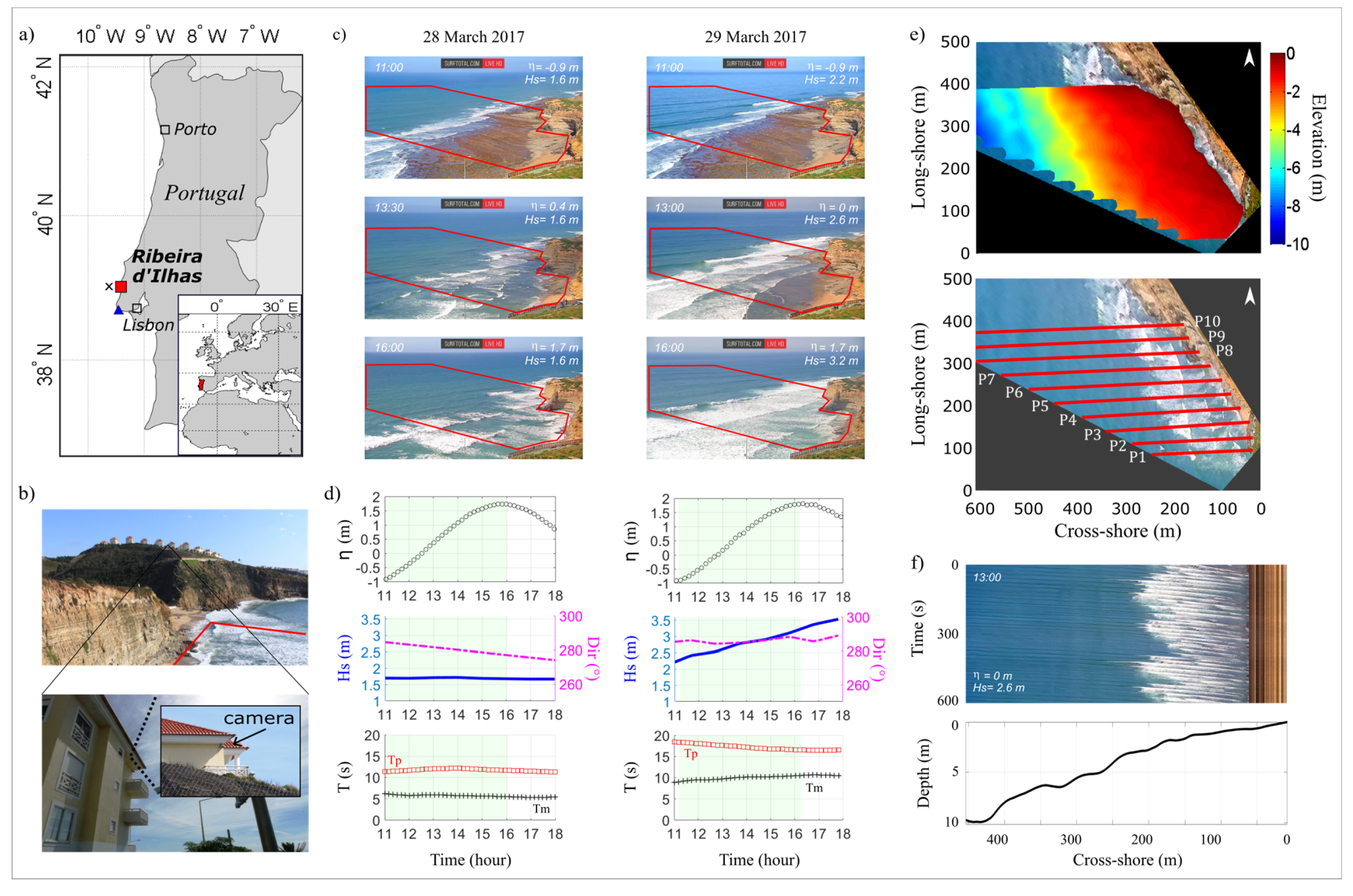
The study area was Ribeira d’Ilhas beach and the adjacent shore (38°59′17.0″N, 9°25′10.4″W) on the North Atlantic Portuguese coast (Figure 1a). The beach stretches approximately 300 m along the shore in a northwest–southeast direction. It is bordered to the south by a 55 m-high cliff and to the north by a headland. The location is well-known as a venue for numerous national and international surfing competitions.

Figure 1.
Study site and video data. (a) Ribeira d’Ilhas beach (red square), tide gauge at Cascais (blue triangle), and SIMAR point for hindcast model (black cross) locations; (b) pictures of the study site taken from North, with red lines indicating a portion of the study area (upper), and camera installation site (lower); (c) snapshots of camera acquisitions during different tidal levels and wave heights over the two considered days. Red contour area indicated the area of interest; (d) hydrodynamic characteristic over the two days, with tide (η), significant wave height (Hs) and wave direction (Dir), wave peak (Tp), and mean (Tm) periods. The shaded green rectangle shows the considered interval of video; (e) ground-truth bathymetry (upper) and transects used for Timestacks production (red lines, named from P1 to P10) on the rectified frame (lower); (f) an example of Timestack image (upper, transect 8 in (e)) and correspondent beach profile (black line, lower).
Through collaboration with Surftotal company (https://www.surftotal.com), video data were obtained from an online-streaming RGB webcam (Figure 1b,c), which provided a fixed view of the Riberia d’Ilhas shore and nearshore for two days (28 and 29 March 2017). The camera was mounted on a house roof approximately 80 m above mean sea level (MSL), located 400 m from the shoreline. Image frames (800 × 450 pixels) were extracted from a total of 12 h of video footage, captured at 5 Hz (5 frames per second) during the rising tide phases on both days (Figure 1d).
Since the camera was installed on private property that was not accessible (Figure 1b), image rectification was carried out using a combination of Cosmos [47] and C-Pro [48] software, along with Ground Control Points collected in the camera field of view during video acquisition. Image distortion induced by the lens was deemed negligible. Further details can be found in Andriolo (2018) [49] and Andriolo et al. (2019) [20].
Each video frame was rectified according to the corresponding tidal level (Figure 1e). Wavefront lines propagating towards the shore were then automatically detected using the method outlined by Andriolo et al. (2020) [50]. This allowed for the selection of 10 cross-shore transects, each spaced 25 m apart along the longshore direction (Figure 1e). To create the Timestack images, pixel arrays were sampled along the selected transects from the rectified 10 min image sequence. The resulting Timestacks covered cross-shore distances between 300 m and 520 m, with a resolution of 1 m per pixel. For each day, 36 Timestacks were generated per transect, leading to a total of 720 Timestacks for the entire dataset (Figure 1f).
The bathymetric profiles for the ten selected transects were derived from the ground-truth nearshore bathymetry map. This map was created by combining a GNSS survey conducted on the low-gradient intertidal slope (tanβ = 0.01) with airborne LiDAR measurements, covering a depth range of 0–10 m (Figure 1e).
Offshore hydrodynamic conditions were retrieved from the hindcast model (www.puertos.es) at the SIMAR point 1042056 (39°N, 9.5°W, Figure 1), while the water-level time series was obtained from the tide gauge of Cascais (38.70°N, 9.43°W, Figure 1). During the rising tide phases (Figure 1d), wave conditions remained relatively stable on the first day, with significant wave height (Hs) of 1.7 m, a peak wave period (Tp) of 11.5 s, and a mean wave period (Tm) of 8 s. On the second day, Hs rose to 3.5 m, Tp decreased from 18 s to 16.5 s, and Tm increased to 10 s (Figure 1d).
2.2. Wave Celerity Assessment from Timestack
In Timestacks, the pixel intensity patterns are related to water elevation, as they reflect the incident light on the water surface. Shoaling waves are represented by darker pixels, which correspond to the shadows cast on the sea surface as waves increase in height over shallow waters. In contrast, the white foam of breaking or broken wave rollers is depicted by brighter pixels [51,52]. Exploiting these properties, an image processing code was developed to extract shoaling and breaking waves patterns, distinctly (Figure 2). The process involved four steps: (i) Pixel intensity correction was applied to the Red band of RGB Timestacks to enhance the contrast between wave patterns and the background; (ii) intensity thresholds were used to distinguish shoaling waves (darker pixel lines) from breaking waves (brighter pixel lines), creating two separate datasets; (iii) a Sobel edge detection filter was applied to each dataset; (iv) lines were extracted in pixel form [51]. A minimum acceptance threshold was implemented to eliminate short-wave patterns and erroneous detections caused by sun glare and cloud shadows. To correct and filter out pixelation noise, a second-order polynomial was fitted to the resulting wave patterns. The final output consisted of lines in the time-space domain, representing individual wave trajectories over the nearshore area (Figure 2).
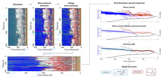
Figure 2.
Wave celerity assessment workflow. After wave pattern detection and fitting, wave celerity is computed as the first derivative for shoaling (blue) and breaking (red) waves. Next, the wave celerity at the breaking points (apparent acceleration) is filtered out using the pixel intensity profile (dashed cyan), whose peak (cyan triangle) identifies the boundary between the outer and inner surf zones (see also [51] for further details). Finally, the celerity profile is used to infer bathymetry using linear and non-linear formulas for shoaling and breaking waves, respectively.
In line with the physical principle that the first derivative of a line in the time-space domain represents the instantaneous speed of a point moving through space, the first derivative was calculated for each wave trajectory to determine the wave celerity of each detected wave (Figure 2). To obtain a representative wave celerity profile, a cross-shore grid with a 2 m spacing was used to compute the median values of wave celerity for both shoaling (cs) and breaking (cb) waves within each 10 min Timestack (Figure 2).
The final step consisted of the integration of cs and cb evaluations to delineate the celerity profile across the entire nearshore domain. The highest peak of the average pixel intensity (Figure 2) was exploited to identify the border between the outer and inner surf zone [51], with cs designated to the outer surf zone, where wave breaking occurs, and cb to the inner surf zone. This methodology allowed for to avoidance of the apparent misleading acceleration returned by wave wave-breaking process [26,53] in celerity computation (Figure 2).
2.3. Depth Inversion
The local depth of the ten profiles (Figure 1e–f) was assessed using the depth inversion technique. The wave celerity is defined by the linear wave dispersion:
where L is the wavelength, g is the acceleration of gravity (=9.81 m/s2), and h is the local depth. Thus, inverting Equation (1), shoaling wave celerity (cs) was used to obtain local water depth hs in the shoaling zone:
with the wavelength L computed iteratively.
In the surf zone, where waves break and non-linear effects of finite wave amplitudes are predominant, an empirical alternative has been proposed to estimate the celerity of breaking waves as follows:
where α is a constant value, commonly proposed as α =1.3 [54]. In this work, we adopted the α value found to best fit the measured breaking wave celerity (cb). Finally, the local depth in the surf zone hb was as follows:
Both hs and hb derived from each Timestack were corrected considering the corresponding tidal level at the Timestack time.
We evaluated the accuracy of the assessments by computing the bias, root mean square error (RMSE), and depth-normalized RMSE (NRMSE) for the ten profiles reconstructed using the depth-inversion technique, comparing them against the ground truth for both days.
3. Results
3.1. Wave Celerity
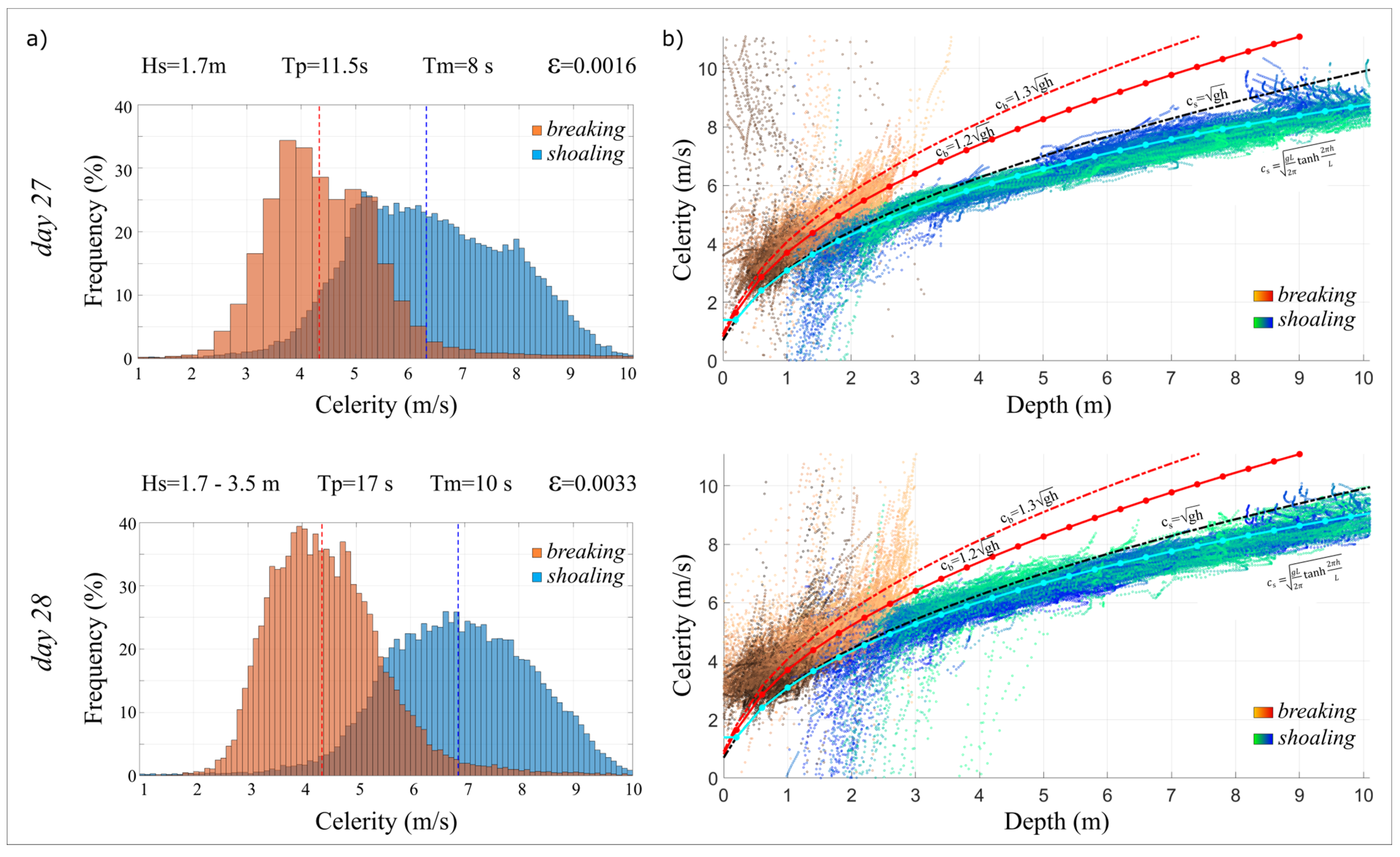
Over the course of the rising tide phases during the two days, the technique provided approximately 150,000 estimated values for shoaling (cs) and 130,000 for breaking (cb) wave celerity from the ten profiles.
The median shoaling celerity values were cs = 6.3 m/s on the first day and cs = 6.9 m/s on the second day, with a standard deviation of σs = 1.45 m/s (Figure 3a). Shoaling celerity was observed to be slower at higher depths during high tide and faster during low tide in the 6–10 m depth range (Figure 3b). In contrast, shoaling wave speeds before breaking were faster at high tide than at low tide for equivalent depths (3–5 m).
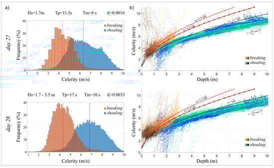
Figure 3.
Wave celerity analysis. (a) Histogram of breaking (orange) and shoaling (blue) wave celerity during the first (upper) and second days (lower). Wave characteristics are also reported, namely, offshore wave height (Hs), peak period (Tp), mean period (Tm), and wave steepness (ε); (b) depth-dependent wave celerity during the first (upper) and second days (lower). The color bars represent sea level, ranging from the lowest (lightest colors) to the highest (darkest colors) tidal elevations, for both breaking (orange to black) and shoaling (green to blue) waves. The graphs also show the modeled celerity for breaking (dotted red lines) and shoaling (dotted black and cyan lines) waves.
Breaking wave celerity values were consistent across both days, with a median value of cb = 4.3 m/s and a standard deviation of σb = 1.1 m/s (Figure 3a). These results are comparable to those obtained by Postacchini and Brocchini (2014) [55] using the cross-correlation technique (cb = 4.47 m/s, σc = 1.09 m/s). The optimal value of α for the breaking wave celerity dataset was determined to be α = 1.2, yielding a goodness-of-fit of R2 = 0.8 [49] (Figure 3b).
3.2. Video-Derived Bathymetry
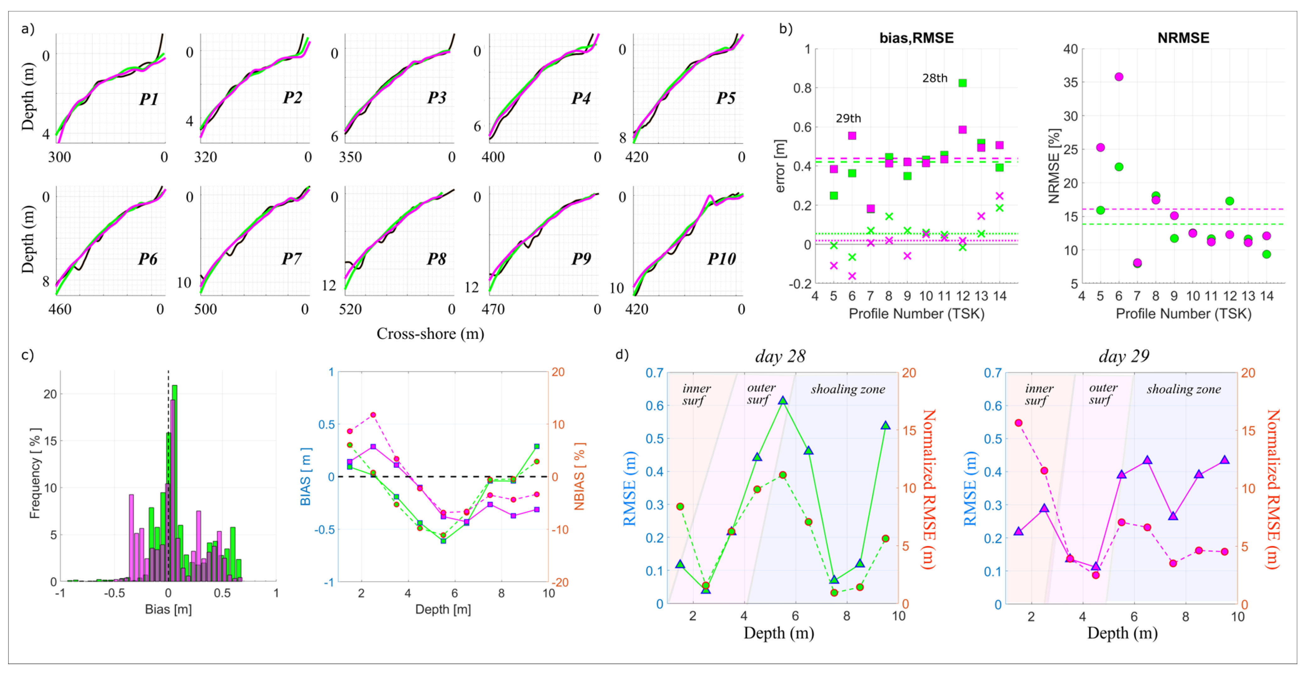
Despite the variation in wave characteristics over the two-day period, the profiles were reproduced with a consistent mean bias of 0.05 m and a mean root mean square error (RMSE) of 0.43 m (Figure 4a). The bias ranged from −0.5 m to 0.5 m, with approximately 51% of the data on the first day and 38% on the second day falling within the range of −0.1 m to 0.1 m (Figure 4a). A slight over-estimation of depth (negative bias) was observed on the profiles closer to the camera (P1–P2). Conversely, a positive bias was observed for the profiles located furthest from the camera (P9–P10). The depth-normalized root mean square error (NRMSE) was generally below 20% for most profiles (Figure 4b).
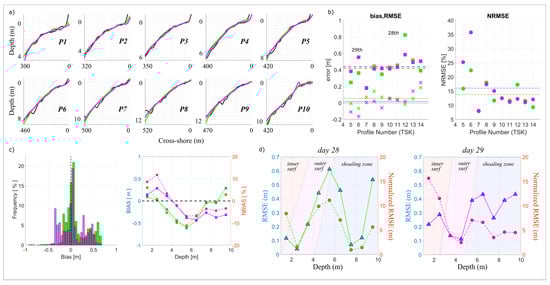
Figure 4.
Depth inversion assessments. (a) Bathymetric profiles (P). The black lines represent the profiles measured using the traditional technique, green and magenta lines show the profiles obtained from the depth inversion method during the first day (28) and the second day (29), respectively; (b) bias and Root Mean Square Error (RMSE) for each profile on both days (left), and depth-normalized NRMSE (right). Dashed lines indicate the median error values; (c) total bias for all profiles (left), along with depth-related and depth-normalized bias (right); (d) RMSE (triangles) and depth-normalized NRMSE (circles) for all profiles across both days. Shaded areas indicate depths associated with different wave transformation zones: inner surf, outer surf, and shoaling zones.
In terms of error dependence on depth, negative bias (overestimation of depth) was noted for most profiles on the first day, while positive bias was observed for depths shallower than 4 m on the second day (Figure 4c). On both days, the highest bias occurred between 5 and 7 m, where the method had difficulty detecting local depressions. However, the normalized bias remained within ±12%. The difficulty in resolving local depressions also led to the highest RMSE values (Figure 4d), which were greater on the first day (0.6 m) than on the second day (0.4 m). Overall, the NRMSE was below 12%, except in the inner surf zone on the second day. Notably, the depths in the outer surf zone were well represented.
4. Discussion
4.1. Wave Celerity
The Timestack-based technique presented here has proven to be an effective method for measuring shoaling and breaking wave celerity in the nearshore zone (Figure 1 and Figure 2). The image processing code used to extract wave patterns can be easily replicated and applied to low-resolution video data. Swell and high wave conditions (Figure 1) were particularly favorable for implementing the methodology, as shoaling wave signatures were clearly visible on Timestacks. However, some adjustments to the algorithm may be required when wave trajectories are less distinct on Timestacks, such as during low-energy sea states. The primary source of detection inaccuracies was the presence of moving clouds and shadows, which altered the pixel brightness on Timestacks (Figure 1c). Although this issue occurred occasionally, the filtering and fitting processes (i) excluded short or unclear wave patterns identified by the image processing algorithm and (ii) removed spurious data resulting from false detections (Figure 2).
Despite the method’s sensitivity to the accurate detection of wave patterns on Timestacks, the results showed strong agreement (Figure 3) with values obtained from field and laboratory data using the cross-correlation technique [31,55,56]. The optimal value of α = 1.2 for breaking wave celerity (Figure 3b) was consistent with values ranging from α = 1.14 to 1.18 observed in other field studies [55,56] and laboratory measurements (α = 1.2, [31]). At the incipient breaking point, wave celerity was found to be approximately twice as fast as predicted by the wave speed model (Figure 3b), likely due to the apparent acceleration of the collapsing wave crest on Timestacks, a phenomenon previously noted by other authors [26,56]. In this context, using pixel intensity variation proved to be an effective method for identifying wave transformation domains [51] and automatically filtering out erroneous breaking wave celerity data in the outer surf zone. This process marked a step forward in obtaining a reliable wave celerity profile (Figure 2) and improving depth inversion accuracy in the outer surf zone (Figure 4). This approach could also be applied to other existing video-based depth inversion techniques [25,27,44].
4.2. Depth Inversion
The study site was well-suited for validating the depth inversion assessments, as the nearshore area was characterized by a stable, non-movable rocky-shore bottom [20,49]. The results obtained were comparable to those from more advanced video-based depth inversion algorithms, which typically show increased inaccuracies with higher wave heights [25,43,44] and/or reduced efficiency in the outer surf zone due to breaking processes [23,53]. It is worth noting that the assessments were considered satisfactory, even with the use of a low-resolution, non-accessible online streaming camera (surfcam), which limited full control over both hydrodynamic and photogrammetric parameters [26,31].
Errors in celerity measurements, and consequently in depth inversion, may be attributable to non-perpendicular Timestack transects to wave direction. Despite the automated detection of wave fronts [50] was helpful in generating perpendicular Timestacks (Figure 1), the wave propagation angle may fluctuate during observations due to variations in sea state and wave refraction/diffraction (Figure 1b). Even though such anomalies constituted spurious data in Ribeira d’Ilhas rocky platform, the technique can be improved by increasing the number of wave fronts sampled over the 10 min period, thereby enhancing the robustness of the wave front direction measurement. A second, alternative approach involves generating Timestacks with constant orientation over time and correcting the computed celerity depending on wave direction [57]. A preliminary test indicated that the Timestack produced with a 75-degree angle (and not 90) with respect to the wave front returned about 10% slower celerity values, suggesting that the trigonometric relation may be used to correct the celerity computed by not-perpendicular Timestacks automatically.
A secondary source of error in the process of depth inversion may be attributable to the use of the mean wave period for the resolution of the linear wave theory (1,2), as the period can change over the monitored period. Therefore, future works may consider retrieving the mean wave period from single Timestacks [58] to enhance the accuracy and representativeness of the actual sea state.
Overall, the method retrieved bathymetric profiles considering video data of 6 h. However, it is possible to achieve assessments with shorter data time intervals. A substantial number of celerity measurements from the same Timestack (Figure 2) could be considered, whereas alternative techniques retrieve a single spatial value [33,35,36]. The acquisition of a robust celerity profile through the utilization of a substantial number of measurements would prove advantageous for the execution of concise video observations, such as those obtained from unmanned aerial vehicles (UAVs) [28,53,59]. The temporal constraints imposed by the limited battery autonomy of commercial devices necessitate the development of efficient data acquisition methodologies, which still have a limited time of acquisition due to limited battery autonomy [60,61,62,63].
The proposed technique was preliminarily tested on a double-barred beach, using images acquired by a video camera that was temporarily installed on the dune crest (Figure 5). Overall, the two bar crests were correctly identified, although the outer bar was spatially shifted offshore due to the low-lying camera and photogrammetry [20,64].
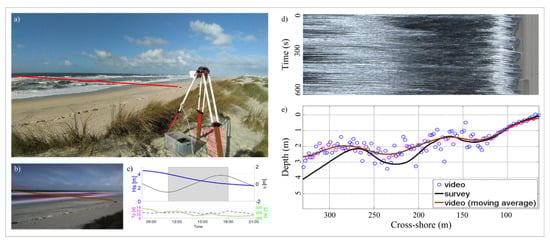
Figure 5.
Preliminary test on a double-barred beach. (a) Overview of the site, with the temporary installation of the camera on the dune crest. The red line indicates the profile considered for testing the video-based depth inversion; (b) example of Timex images produced over 10 min time interval. The red line indicates the profile considered for testing the video-based depth inversion; (c) hydrodynamic condition during the experiment, with significant wave height (Hs), sea level (η), peak wave period (Tp), and wave direction (Dir). Grey background indicates the interval of camera recording (6 h); (d) example of Timestack image produced over the considered transect during 10 min time interval; (e) depth inversion results (blue circles and red line) plotted over the profile (black line) surveyed by a jet-sky before the video experiment.
5. Conclusions
The present study proposed a video-based methodology for measuring nearshore wave celerity and inferring shallow water bathymetry. Distinct shoaling and breaking wave patterns were identified in Timestack images, enabling the estimation of wave celerity across different nearshore wave domains.
The depth inversion of ten cross-shore bathymetric profiles, with a maximum depth of 10 m, showed a mean bias of 0.05 m and a root mean square error (RMSE) of 0.43 m. These achievements underscore the efficacy in retrieving bathymetry in the outer surf zone (depth-normalized RMSE = 15%), where the breaking wave process occurs. In this regard, the methodology has the potential to advance the depth inversion on barred beaches and during high-energy events.
The developed technique can be implemented in the analysis of images obtained from operational coastal monitoring stations globally, with its applicability extending to drone video acquisitions. Finally, it is proposed that a component of the methodology could be integrated into extant Timestack-based techniques for enhancing depth inversion in the outer surf zone.
Author Contributions
Conceptualization, U.A., A.A., and R.T.; methodology, U.A., A.A., and R.T.; software, U.A., A.A., and R.T.; validation, U.A.; formal analysis, U.A.; investigation, U.A., A.A., and R.T.; resources, U.A., G.G., and R.T.; data curation, U.A. and A.A.; writing—original draft preparation, U.A.; writing—review and editing, U.A., A.A., G.G., and R.T.; visualization, U.A. and A.A.; supervision, G.G. and R.T.; project administration, G.G. and R.T.; funding acquisition, G.G. and R.T. All authors have read and agreed to the published version of the manuscript.
Funding
The work was partially supported by the EARTHSYSTEM Doctorate Programme (SFRH/BD/52558/2014) and by the Portuguese Foundation for Science and Technology (FCT) Operational Program for Competitiveness and Internationalization (POCI) in the frameworks of Pluriannual Funding UID/308 (Instituto de Engenharia de Sistemas e Computadores de Coimbra—INESC Coimbra) and UIDB/50019/2020. This work was also supported by the Alliance for the Energy Transition (56) co-financed by the Recovery and Resilience Plan (PRR) through the European Union.
Data Availability Statement
Data will be available upon request.
Acknowledgments
The authors warmly acknowledge Cristina Lira, André Fortunato, and Diogo Mendes for their support during fieldwork, Ana Bastos for providing LiDAR bathymetry data, and Elena Sánchez-García for the help in rectifying the surfcam images. The authors also wish to thank FCT projects held by LNEC: To-SEAlert (PTDC/EAM-OCE/31207/2017) and BSafe4Sea (PTDC/ECI-EGC/31090/2017).
Conflicts of Interest
The authors declare no conflicts of interest.
References
- Fontán-Bouzas, Á.; Alcántara-Carrió, J.; Albarracín, S.; Baptista, P.; Silva, P.A.; Portz, L.; Manzolli, R.P. Multiannual shore morphodynamics of a Cuspate Foreland: Maspalomas (Gran Canaria, Canary Islands). J. Mar. Sci. Eng. 2019, 7, 416. [Google Scholar] [CrossRef]
- Melet, A.; Teatini, P.; Le Cozannet, G.; Jamet, C.; Conversi, A.; Benveniste, J.; Almar, R. Earth Observations for Monitoring Marine Coastal Hazards and Their Drivers. Surv. Geophys. 2020, 41, 1489–1534. [Google Scholar] [CrossRef]
- Mendes, D.; Pinto, J.P.; Pires-Silva, A.A.; Fortunato, A.B. Infragravity wave energy changes on a dissipative barred beach: A numerical study. Coast. Eng. 2018, 140, 136–146. [Google Scholar] [CrossRef]
- Zijlema, M.; Stelling, G.; Smit, P. SWASH: An operational public domain code for simulating wave fields and rapidly varied flows in coastal waters. Coast. Eng. 2011, 58, 992–1012. [Google Scholar] [CrossRef]
- Booij, N.; Holthuijsen, L.H.; Ris, R.C. The “Swan” Wave Model for Shallow Water. Coast. Eng. 1997, 1, 510–516. [Google Scholar]
- Ciavola, P.; Ferreira, O.; Van Dongeren, A.; Van Thiel de Vries, J.; Armaroli, C.; Harley, M. Prediction of Storm Impacts on Beach and Dune Systems. In Hydrometeorological Hazards: Interfacing Science and Policy; John Wiley and Sons: Hoboken, NJ, USA, 2014; Volume 9781118629, pp. 227–252. ISBN 9781118629567. [Google Scholar]
- Garnier, E.; Ciavola, P.; Spencer, T.; Ferreira, O.; Armaroli, C.; McIvor, A. Historical analysis of storm events: Case studies in France, England, Portugal and Italy. Coast. Eng. 2018, 134, 10–23. [Google Scholar] [CrossRef]
- Matias, A.; Rita Carrasco, A.; Loureiro, C.; Masselink, G.; Andriolo, U.; McCall, R.; Ferreira, Ó.; Plomaritis, T.A.; Pacheco, A.; Guerreiro, M. Field measurements and hydrodynamic modelling to evaluate the importance of factors controlling overwash. Coast. Eng. 2019, 152, 103523. [Google Scholar] [CrossRef]
- Ferreira, Ó. Modelling Risk Reduction Measures to Minimise Future Impacts of Storms at Coastal Areas. In Springer Climate; Springer: Berlin/Heidelberg, Germany, 2022. [Google Scholar]
- Mentaschi, L.; Vousdoukas, M.I.; Pekel, J.F.; Voukouvalas, E.; Feyen, L. Global long-term observations of coastal erosion and accretion. Sci. Rep. 2018, 8, 12876. [Google Scholar] [CrossRef]
- Masselink, G.; Van Heteren, S. Response of wave-dominated and mixed-energy barriers to storms. Mar. Geol. 2014, 352, 321–347. [Google Scholar] [CrossRef]
- Fontán, A.; Alcántara-Carrió, J.; Correa, I.D. Combined beach—Inner shelf erosion in short and medium term (Maspalomas, Canary Islands). Geol. Acta 2012, 10, 411–426. [Google Scholar]
- Salameh, E.; Frappart, F.; Almar, R.; Baptista, P.; Heygster, G.; Lubac, B.; Raucoules, D.; Almeida, L.P.; Bergsma, E.W.J.; Capo, S.; et al. Monitoring Beach Topography and Nearshore Bathymetry Using Spaceborne Remote Sensing: A Review. Remote Sens. 2019, 11, 2212. [Google Scholar] [CrossRef]
- Kutser, T.; Hedley, J.; Giardino, C.; Roelfsema, C.; Brando, V.E. Remote sensing of shallow waters—A 50 year retrospective and future directions. Remote Sens. Environ. 2020, 240, 111619. [Google Scholar] [CrossRef]
- Almeida, L.P.; Almar, R. Application of remote sensing methods to monitor coastal zones. J. Mar. Sci. Eng. 2020, 8, 391. [Google Scholar] [CrossRef]
- Pacheco, A.; Horta, J.; Loureiro, C. Ferreira Retrieval of nearshore bathymetry from Landsat 8 images: A tool for coastal monitoring in shallow waters. Remote Sens. Environ. 2015, 159, 102–116. [Google Scholar] [CrossRef]
- Turner, I.L.; Harley, M.D.; Almar, R.; Bergsma, E.W.J. Satellite optical imagery in Coastal Engineering. Coast. Eng. 2021, 167, 103919. [Google Scholar] [CrossRef]
- Catalán, P.; Haller, M.C. Nonlinear phase speeds and depth inversions. Coast. Dyn. 2005 Proc. Fifth Coast. Dyn. Int. Conf. 2006, 1–14. [Google Scholar]
- Almar, R.; Bergsma, E.W.J.; Thoumyre, G.; Baba, M.W.; Cesbron, G.; Daly, C.; Garlan, T.; Lifermann, A. Global satellite-based coastal bathymetry from waves. Remote Sens. 2021, 13, 4628. [Google Scholar] [CrossRef]
- Andriolo, U.; Sánchez-García, E.; Taborda, R. Operational use of surfcam online streaming images for coastal morphodynamic studies. Remote Sens. 2019, 11, 78. [Google Scholar] [CrossRef]
- Splinter, K.D.; Harley, M.D.; Turner, I.L. Remote sensing is changing our view of the coast: Insights from 40 years of monitoring at Narrabeen-Collaroy, Australias. Remote Sens. 2018, 10, 1744. [Google Scholar] [CrossRef]
- Holman, R.A.; Stanley, J. The history and technical capabilities of Argus. Coast. Eng. 2007, 54, 477–491. [Google Scholar] [CrossRef]
- Stockdon, H.F.; Holman, R.A. Estimation of wave phase speed and nearshore bathymetry from video imagery. J. Geophys. Res. Ocean. 2000, 105, 22015–22033. [Google Scholar] [CrossRef]
- Zikra, M. Development of Video Image Analysis Methods for Estimating Bathymetry and the Directional Wave Spectrum in Shallow Water Areas. Ph.D. Thesis, Kyushu university, Fukuoka, Japan, 2012. [Google Scholar]
- Holman, R.; Plant, N.; Holland, T. CBathy: A robust algorithm for estimating nearshore bathymetry. J. Geophys. Res. Ocean. 2013, 118, 2595–2609. [Google Scholar] [CrossRef]
- Catálan, P.A.; Haller, M.C. Remote sensing of breaking wave phase speeds with application to non-linear depth inversions. Coast. Eng. 2008, 55, 93–111. [Google Scholar] [CrossRef]
- Simarro, G.; Calvete, D.; Luque, P.; Orfila, A.; Ribas, F. UBathy: A new approach for bathymetric inversion from video imagery. Remote Sens. 2019, 11, 2722. [Google Scholar] [CrossRef]
- Gawehn, M.; De Vries, S.; Aarninkhof, S. A self-adaptive method for mapping coastal bathymetry on-the-fly from wave field video. Remote Sens. 2021, 13, 4742. [Google Scholar] [CrossRef]
- Santos, D.; Abreu, T.; Silva, P.A.; Baptista, P. Estimation of coastal bathymetry using wavelets. J. Mar. Sci. Eng. 2020, 8, 772. [Google Scholar] [CrossRef]
- Santos, D.; Abreu, T.; Silva, P.A.; Santos, F.; Baptista, P. Nearshore Bathymetry Retrieval from Wave-Based Inversion for Video Imagery. Remote Sens. 2022, 14, 2155. [Google Scholar] [CrossRef]
- Almar, R.; Cienfuegos, R.; Catalán, P.A.; Birrien, F.; Castelle, B.; Michallet, H. Nearshore bathymetric inversion from video using a fully non-linear Boussinesq wave model. J. Coast. Res. 2011, 64, 3–7. [Google Scholar]
- Liu, H.; Arii, M.; Sato, S.; Tajima, Y. Long-Term Nearshore Bathymetry Evolution From Video Imagery: A Case Study in the Miyazaki Coast. Coast. Eng. Proc. 2012, 1, 60. [Google Scholar] [CrossRef]
- Almar, R.; Bonneton, P.; Senechal, N.; Roelvink, D. Wave Celerity From Video Imaging: A New Method. Coast. Eng. 2009, 661–673. [Google Scholar]
- Almar, R. Morphodynamique Littorale Haute Fréquence par Imagerie Vidéo. Ph.D. Thesis, Université de Rouen, Mont-Saint-Aignan, France, 2009. [Google Scholar]
- Abessolo, G.O.; Almar, R.; Bonou, F.; Bergsma, E. Error Proxies in Video-Based Depth Inversion: Temporal Celerity Estimation. J. Coast. Res. 2020, 95, 1101. [Google Scholar] [CrossRef]
- Thuan, D.H.; Almar, R.; Marchesiello, P.; Viet, N.T. Video Sensing of Nearshore Bathymetry Evolution with Error Estimate. J. Mar. Sci. Eng. 2019, 7, 233. [Google Scholar] [CrossRef]
- Tsukada, F.; Shimozono, T.; Matsuba, Y. UAV-based mapping of nearshore bathymetry over broad areas. Coast. Eng. J. 2020, 62, 285–298. [Google Scholar] [CrossRef]
- Hashimoto, K.; Shimozono, T.; Matsuba, Y.; Okabe, T. Unmanned aerial vehicle depth inversion to monitor river-mouth bar dynamics. Remote Sens. 2021, 13, 412. [Google Scholar] [CrossRef]
- Yoo, J.; Fritz, H.M.; Haas, K.A.; Work, P.A.; Barnes, C.F. Depth Inversion in the Surf Zone with Inclusion of Wave Nonlinearity Using Video-Derived Celerity. J. Waterw. Port. Coast. Ocean. Eng. 2011, 137, 95–106. [Google Scholar] [CrossRef]
- Yoo, J.; Fritz, H. Nonlinear Bathymetry Inversion Based on Wave Property Estimation from Nearshore Video Imagery. Civ. Environ. Engng. 2007. [Google Scholar]
- Matsuba, Y.; Sato, S. Nearshore bathymetry estimation using UAV. Coast. Eng. J. 2018, 60, 51–59. [Google Scholar] [CrossRef]
- Palmsten, M.L.; Brodie, K.L. The Coastal Imaging Research Network (CIRN). Remote Sens. 2022, 14, 453. [Google Scholar] [CrossRef]
- Brodie, K.L.; Palmsten, M.L.; Hesser, T.J.; Dickhudt, P.J.; Raubenheimer, B.; Ladner, H.; Elgar, S. Evaluation of video-based linear depth inversion performance and applications using altimeters and hydrographic surveys in a wide range of environmental conditions. Coast. Eng. 2018, 136, 147–160. [Google Scholar] [CrossRef]
- Rodríguez-Padilla, I.; Castelle, B.; Marieu, V.; Morichon, D. Video-Based Nearshore Bathymetric Inversion on a Geologically Constrained Mesotidal Beach during Storm Events. Remote Sens. 2022, 14, 3850. [Google Scholar] [CrossRef]
- Bouvier, C.; Balouin, Y.; Castelle, B.; Valentini, N. Video Depth Inversion at a Microtidal Site Exposed to Prevailing Low-energy Short-period Waves and Episodic Severe Storms. J. Coast. Res. 2020, 95, 1021–1026. [Google Scholar] [CrossRef]
- Bergsma, E.W.J.J.; Almar, R. Video-based depth inversion techniques, a method comparison with synthetic cases. Coast. Eng. 2018, 138, 199–209. [Google Scholar] [CrossRef]
- Taborda, R.; Silva, A. COSMOS: A lightweight coastal video monitoring system. Comput. Geosci. 2012, 49, 248–255. [Google Scholar] [CrossRef]
- Sánchez-García, E.; Balaguer-Beser, A.; Pardo-Pascual, J.E. C-Pro: A coastal projector monitoring system using terrestrial photogrammetry with a geometric horizon constraint. ISPRS J. Photogramm. Remote Sens. 2017, 128, 255–273. [Google Scholar] [CrossRef]
- Andriolo, U. Nearshore Hydrodynamics and Morphology Derived from Video Imagery; Faculdade de Ciências da Universidade de Lisboa: Lisbon, Portugal, 2018. [Google Scholar]
- Andriolo, U.; Mendes, D.; Taborda, R. Breaking wave height estimation from timex images: Two methods for coastal video monitoring systems. Remote Sens. 2020, 12, 204. [Google Scholar] [CrossRef]
- Andriolo, U. Nearshore wave transformation domains from video imagery. J. Mar. Sci. Eng. 2019, 7, 186. [Google Scholar] [CrossRef]
- Almar, R.; Cienfuegos, R.; Catalán, P.A.; Michallet, H.; Castelle, B.; Bonneton, P.; Marieu, V. A new breaking wave height direct estimator from video imagery. Coast. Eng. 2012, 61, 42–48. [Google Scholar] [CrossRef]
- Bergsma, E.W.J.; Almar, R.; Melo de Almeida, L.P.; Sall, M. On the operational use of UAVs for video-derived bathymetry. Coast. Eng. 2019, 152, 103527. [Google Scholar] [CrossRef]
- Madsen, P.A.; Sørensen, O.R.; Schäffer, H.A. Surf zone dynamics simulated by a Boussinesq type model. Part II: Surf beat and swash oscillations for wave groups and irregular waves. Coast. Eng. 1997, 32, 289–319. [Google Scholar] [CrossRef]
- Postacchini, M.; Brocchini, M. A wave-by-wave analysis for the evaluation of the breaking-wave celerity. Appl. Ocean. Res. 2014, 46, 15–27. [Google Scholar] [CrossRef]
- Tissier, M.; Bonneton, P.; Almar, R.; Castelle, B.; Bonneton, N.; Nahon, A. Field measurements and non-linear prediction of wave celerity in the surf zone. Eur. J. Mech. B/Fluids 2011, 30, 635–641. [Google Scholar] [CrossRef]
- Perugini, E.; Soldini, L.; Palmsten, M.L.; Calantoni, J.; Brocchini, M. Linear depth inversion sensitivity to wave viewing angle using synthetic optical video. Coast. Eng. 2019, 152, 103535. [Google Scholar] [CrossRef]
- Osorio, A.F.; Montoya-Vargas, S.; Cartagena, C.A.; Espinosa, J.; Orfila, A.; Winter, C. Virtual BUOY: A video-based approach for measuring near-shore wave peak period. Comput. Geosci. 2019, 133, 104302. [Google Scholar] [CrossRef]
- Sun, S.-H.; Chuang, W.-L.; Chang, K.-A.; Young Kim, J.; Kaihatu, J.; Huff, T.; Feagin, R. Imaging-Based Nearshore Bathymetry Measurement Using an Unmanned Aircraft System. J. Waterw. Port. Coast. Ocean. Eng. 2019, 145, 04019002. [Google Scholar] [CrossRef]
- Gonçalves, G.; Gonçalves, D.; Gómez-gutiérrez, Á.; Andriolo, U.; Pérez-alvárez, J.A. 3D reconstruction of coastal cliffs from fixed-wing and multi-rotor uas: Impact of sfm-mvs processing parameters, image redundancy and acquisition geometry. Remote Sens. 2021, 13, 1222. [Google Scholar] [CrossRef]
- Gonçalves, D.; Gonçalves, G.; Pérez-Alvávez, J.A.; Andriolo, U. On the 3D Reconstruction of Coastal Structures by Unmanned Aerial Systems with Onboard Global Navigation Satellite System and Real-Time Kinematics and Terrestrial Laser Scanning. Remote Sens. 2022, 14, 1485. [Google Scholar] [CrossRef]
- Andriolo, U.; Garcia-Garin, O.; Vighi, M.; Borrell, A.; Gonçalves, G. Beached and Floating Litter Surveys by Unmanned Aerial Vehicles: Operational Analogies and Differences. Remote Sens. 2022, 14, 1336. [Google Scholar] [CrossRef]
- Gonçalves, D.; Gonçalves, G.; Pérez-Alvárez, J.A.; Andriolo, U. 3D cliff reconstruction by drone: An in-depth analysis of the image network. Meas. J. Int. Meas. Confed. 2023, 222, 113606. [Google Scholar] [CrossRef]
- Catalán, P.A.; Haller, M.C.; Holman, R.A.; Plant, W.J. Optical and microwave detection of wave breaking in the surf zone. IEEE Trans. Geosci. Remote Sens. 2011, 49, 1879–1893. [Google Scholar] [CrossRef]


Disclaimer/Publisher’s Note: The statements, opinions and data contained in all publications are solely those of the individual author(s) and contributor(s) and not of MDPI and/or the editor(s). MDPI and/or the editor(s) disclaim responsibility for any injury to people or property resulting from any ideas, methods, instructions or products referred to in the content. |
© 2025 by the authors. Licensee MDPI, Basel, Switzerland. This article is an open access article distributed under the terms and conditions of the Creative Commons Attribution (CC BY) license (https://creativecommons.org/licenses/by/4.0/).