Abstract
Sea Surface Salinity is a crucial climatic variable due to its twofold role as both a passive and an active tracer of oceanic processes. Despite its relevance, however, it could not be measured from space, mainly because of technological limitations, until 2009. Since then, the generation and assessment of satellite salinity has become a game-changer in physical and biogeochemical oceanography, as well as in climate science. Three satellite sensors with salinity-measuring capabilities (SMOS-Soil Moisture and Ocean Salinity, Aquarius, and SMAP-Soil Moisture Active Passive) have been launched in the previous decade, each characterized by specific measurement concepts and features and ad hoc validation approaches. The increasing usage of spaceborne salinity products has produced a variety of results and applications, which are here summarized under three specific domains: climate, scientific, and operational. Finally, short-to-mid-term perspectives, indicating both the expected improvements in terms of algorithms and also looking at novel mission concepts (that will provide continuation of these measurements in the decade to come) have been described.
Keywords:
Sea Surface Salinity; Earth Observation; SMOS; Aquarius; SMAP; radiometry; oceanography; climate 1. Sea Surface Salinity: Background and Ongoing Efforts
Sea Surface Salinity (SSS) is a crucial environmental and climatic variable due to its twofold role as both a passive and an active tracer of oceanic processes. Despite its relevance, however, it has not been measurable from space, mainly because of technological limitations, up to the advent of the first satellite with this capability, in 2009.
The “Oceans from Space” conference series, which reviews progress and challenges in the satellite oceanography field with a decadal pace [1], tracked the development of SSS remote sensing since its inception. At the conference held in 2000, a friendly wager on the future of spaceborne satellites was made among the conference participants [2], foreseeing a bright future for technologies aiming at addressing SSS from space. At the subsequent 2010 edition, reflections on that wager were elaborated by the Principal Investigators of the recently launched Soil Moisture and Ocean Salinity (SMOS) mission and the soon-to-be-launched Aquarius mission, focusing on the challenges and excitement of the first-ever salinity measurements from space [3]. At the 2020 conference (deferred to October 2022 due to the COVID-19 pandemic restrictions), a compendium of a full decade of achievements in the broad oceanographic and climate perspective was presented [4], stressing how decisive the impact of SSS remote sensing actually was and currently is. Feedback was also gathered on residual concerns and limitations, as well as on future developments.
In this paper, we take stock of the broad scientific advancements and related discussions, assessing to what extent salinity from satellites has been a game-changer in physical and biogeochemical oceanography, and in climate science at large. After describing the three satellite sensors with salinity-measuring capabilities deployed so far—SMOS; Aquarius; and Soil Moisture Active Passive (SMAP)—along with their measurement concepts and features; the related validation approaches; and the inventory of products generated; we shall concentrate on the portfolio of scientific results that have been obtained by exploiting these data sources. The results will be opportunely divided into climate, scientific, and operational applications. Lastly, we will focus on the short-to-mid-term perspectives, indicating the expected improvements in terms of algorithms, but also looking at novel mission concepts that will provide continuity and enhancement to these measurements in the next decade. The focus of the present review is intentionally broad but necessarily succinct to cover the ample variety of studies on oceanic processes that were initiated, enhanced, or better characterized by the increasingly accurate and de-biased continuous stream of SSS data from the available variety of platforms and sensors.
1.1. Ocean Salinity Relevance in Oceanography and Water Cycle
The salinity of marine waters has long been recognized as a crucial parameter in the monitoring, diagnosis, and understanding of oceanic processes. In recognition of its relevance, it has been labeled as an Essential Climate Variable (ECV) and Essential Ocean Variable (EOV) by the Global Climate Observing System (GCOS) and Global Ocean Observing System (GOOS) committees [5]. SSS has a prominent role as a passive tracer, being the resulting diagnostic of the interplay between evaporation and precipitation and, in specific areas, of the additional influence of formation/melting of ice and freshwater runoff, together with horizontal/vertical advection. As such, salinity relevance within the water cycle is critical. Besides, salinity also plays an active tracer role, whereas horizontal and vertical variations of salinity might imply a change in seawater density and therefore indicate a possible trigger of the thermohaline circulation.
The advent of salinity-measuring satellites since the end of the 2000s (Figure 1) has dramatically reduced the observing-system capability gaps, given that the existing Argo floats, although essential, were insufficient to resolve salinity features with spatial scales smaller than hundreds of km and time scales of less than a month [6].
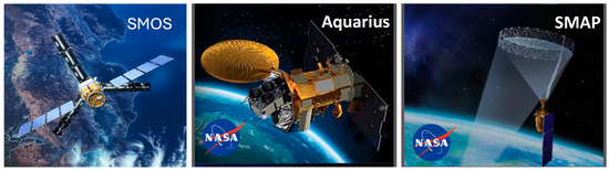
Figure 1.
Artistic view of the three L-band satellite radiometers measuring sea surface salinity. From left to right: SMOS, Aquarius, and SMAP.
Before the launch of current satellite SSS sensors, and as repeatedly discussed at the early Oceans from Space conferences recalled above, it was anticipated that the synoptic and frequent monitoring of this parameter from space, in spite of the limitations of a coarse spatial resolution and the inherent noise and biases, might prove essential in giving insights into various aspects of oceanography and climate, such as (and not limited to) air-sea interactions, river discharge monitoring, ocean dynamics, mesoscale characterization, ocean modeling, and so forth.
1.2. Satellite SSS Sensors and Measurement Principles/Challenges (SMOS, Aquarius, SMAP)
1.2.1. SMOS
The Soil Moisture and Ocean Salinity (SMOS) is a European Space Agency (ESA) Earth Explorer opportunity mission [7]. It was launched in November 2009, with a nominal lifetime of 3–5 years, currently extended until the end of 2025, with a recent request for continuation up until 2028. It was a proof of concept of a novel Earth Observation (EO) technique demonstration: microwave radiometry by aperture synthesis.
SMOS is the first L-band radiometer in space, achieving global and continuous coverage. It was also the first satellite to infer SSS, as well as Soil Moisture (a land hydrology variable not covered in the present paper), directly and in an absolute fashion. The 2D interferometer was conceived to provide fully polarized multi-angular measurements of the surface, with a native spatial resolution of about 30 km at 3 dB below the satellite and 43 km on average over the whole field of view, sampled over the ISEA 4H9 Discrete Global Grid (DGG) at 15 km resolution [8]. The L-band channel was selected as the best compromise among minimum atmospheric effect, reasonable spatial resolution, and maximum sensitivity to the target variable of ocean salinity. However, being the first L-band mission to be deployed in space, it experienced an unexpectedly high level of Radio Frequency Interference (RFI) in the supposedly protected 1400–1427 MHz band [9], which called for sustained efforts over the years in devising mitigation and filtering techniques, and that was also instrumental in the design of the forthcoming L-band sensors.
The mission design allows global coverage of the Earth in less than 3 days at the equator, with a dusk/dawn orbit to minimize temperature gradients at the ocean-atmosphere interface. The rationale of SSS retrieval exploits the variation of the seawater conductivity properties with salinity, which in turn affects the emissivity and ultimately the Brightness Temperature (TB) measured with microwave radiometers. Specifically, the multangular acquisition of TBs over the so-called dwell-line is translated into a single SSS estimate in each pixel once the contribution of additional auxiliary data that also affect the TB value—namely; Sea Surface Temperature (SST); and Wind Speed (WS) as prime descriptors of sea roughness—are also accounted for [10,11,12]. Regarding the latter, colocation/uncertainty of the needed auxiliary data of SST and WS are also crucial. Parametrizations of the dielectric constant model [13] and of the emissivity of the sea surface due to roughness and foam have been constantly improving [14], alongside a debiasing module known as Ocean Target Transformation (OTT) [15]. In recent years, an empirical correction to handle the land signal leakage into the sea scenes that was jeopardizing measurements in the coastal ocean has been devised and implemented: The so-called Land-Sea Contamination (LSC) correction [16]. As such, both uncorrected and corrected salinity fields are served. Moreover, additional perturbation sources such as Galactic noise and Sun glint have been addressed with a set of algorithms that are still evolving. To date, three overall reprocessing campaigns have been carried out, and a fourth one is imminent.
ESA delivers both SMOS L1 and L2 products. Level 1 is multi-angular fully polarized TB, and Level 2 products over the ocean are organized by ascending and descending half-orbits SSS. Level 3 SSS global maps are produced operationally in various research and operational centers, as described afterwards. The prescribed mission accuracy is defined at L3, with SSS aimed to be 0.1 pss STDD (Standard Deviation of the Difference) over a 200 × 200 km spatial scale and over a month window [17].
1.2.2. Aquarius
The joint National Aeronautics and Space Administration (NASA) and Comisíon Nacional de Actividades Espaciales (CONAE) Aquarius mission [18] was launched on the Satélite de Aplicaciones Científicas (SAC)-D spacecraft, provided by Argentina’s space agency, in June 2011. It carried a real aperture L-band radiometer and a scatterometer as the primary sensors. The main scientific objectives were to measure SSS over the global ice-free oceans with a 150 km spatial resolution for a 7-day revisit and to achieve a measurement accuracy of less than 0.2 pss on a 30-day time scale, taking into account all sensor and geophysical random errors and biases. Due to an electronic failure on the platform, the Aquarius mission ended prematurely in June 2015. Aquarius Level 3 from NASA (version 5) is the reference end-of-mission data release of the Aquarius/SAC-D mission.
The Aquarius instrument had an onboard Radio Frequency Interference (RFI) filtering system, which took stock of the RFI pollution contaminating SMOS measurements [19]. The unique capability of Aquarius was the availability of an L-band scatterometer onboard, which could be used to provide coincident estimates of the ocean’s surface roughness, overcoming one of the hurdles of both SMOS and later SMAP, that is, the spatio-temporal collocation of parameters suitable to correct for the roughness effect on the ocean emissivity.
1.2.3. SMAP
The SMAP mission [20], jointly developed by NASA and the Jet Propulsion Laboratory (JPL), was launched in January 2015. SMAP included originally an L-band radar and an L-band radiometer for concomitant active/passive measurements. The radiometer and radar instruments became operational in April 2015. The radar transmitter regrettably ceased operating only a few months after (in July 2015) due to a hardware glitch, and therefore the radiometer remained the only operational instrument collecting science observations [21].
SMAP employs a 6 m rotating mesh antenna, which provides a wide swath coverage (of about 1000 km), obtaining TB observations at an effective resolution close to 43 km [21]. Benefiting from lessons learned by the SMOS and Aquarius missions, the SMAP receivers have the ability to record time–frequency sub-band data in order to detect emission contamination caused by manmade sources of RFI [22].
The SMAP science data products are provided with different granularity. Operationally, the Level 1 products are TB observations from the radiometer arranged in ascending and descending half-orbits. Specifically, these are the Level 1B geolocated TBs and the Level 1C TBs resampled on the Equal-Area Scalable Earth (EASE)-Grid map projections at 9 km and 36 km grid resolutions. The Level 2 products over the ocean are swath-based salinity produced in two institutions, i.e., Remote Sensing Systems (RSS) and JPL.
1.3. Features of the Current Version of the Satellite Salinity Mission Processors
Over the last decade, space agencies issued different releases of their salinity products to reflect the continuous research and development on both the algorithmic side and on the correction of the numerous signal perturbations.
Regarding SMOS, several data product versions have been deployed in the official ESA baseline (Figure 2), associated with three overall archive reprocessing campaigns performed to ensure consistency of the whole dataset. These versions aimed at refining the geophysical forward models, at providing improved versions for dielectric constant models, at devising specific corrections to tackle the perturbing effects of sky, sun, and galactic glints, at addressing instrument biases propagating at L2, and at mitigating the effect of RFI.
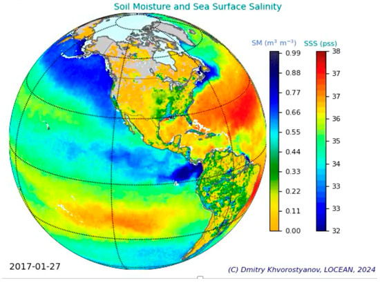
Figure 2.
Composite of the two water-cycle-related parameters—soil moisture and ocean salinity—for a sample date in 2017. Over the ocean, visible patterns of high salinity are reflecting the evaporative gyres in the Atlantic and tropical Pacific, while low salinity is associated with the ITCZ (Inter-Tropical Convergence Zone) or high latitudes.
The latest SMOS version that is operational is v700, featuring a novel dielectric constant model [13], an improved computation of a de-biased salinity anomaly (with respect to a self-consistent SMOS climatology), an improved estimation of the auxiliary data errors, and an improved characterization of the L2 SSS uncertainty. Upcoming versions, which will soon undergo a 4th SMOS mission reprocessing, are now dealing with an improved correction to mitigate the influence of ice contamination and ad hoc corrections for latitudinal and seasonal biases experienced in the measurements. An alternative retrieval scheme based on a novel algorithm, the so-called Debiased non-Bayesian-DnB [23], has been implemented and is subject to a dedicated round-robin comparison exercise to assess its merits and limitations as compared to the nominal inversion scheme.
1.4. Mission Supporting Field Campaigns
A variety of experimental field campaigns supporting pre-launch simulations, modelling advancements, and error characterization took place in the decade preceding the satellite’s launch, such as WISE, FROG, CAROL, and COSMOS (to name just a few), whose major outcomes are summarized in [24]. In the last decade, two major comprehensive field experiments funded by NASA took place, the so-called Salinity Processes in the Upper-ocean Regional Study (SPURS). Namely, SPURS-1 [25] and SPURS-2 [26] were two process studies aiming at characterizing dynamics in two different regimes, one dominated by evaporation and the other one dominated by precipitation. The results were compiled in [27,28] and helped shed light on various processes dominated or mediated by SSS.
More recently, an intense field campaign activity, funded by NASA, the Salinity and Stratification at the Sea Ice Edge (SASSIE) experiment, was performed in 2022 to enhance the understanding of polar-ocean and sea-ice dynamics. SASSIE has been a comprehensive experiment with consistent deployment of instrumentation and collection of a wealth of in-situ data. A strong emphasis was given to instrumentations able to capture the skin surface salinity, being therefore comparable to satellite measurements and advancing in the characterization of the vertical mismatch problem (Figure 3). Most notably, SASSIE was aiming at investigating how the salinity patterns could be helpful in the prediction of the extent and timing of subsequent sea-ice formation in the Arctic region. A campaign dataset [29] and a dedicated website are currently available, while a specific experiment was recently carried out to build a machine-learning algorithm aimed at inferring sea-ice formation timing out of salinity inputs. Preliminary results indicate that, when including L4 merged salinity products, the estimation of sea-ice formation/retreat is remarkably improving, paving the way to new applications of salinity as a prognostic variable.
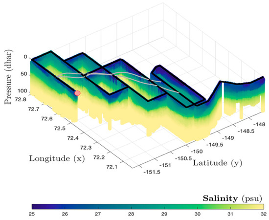
Figure 3.
Three-dimensional plot showing salinity evolution over latitude, longitude, and depth for a transect in the SASSIE campaign (credits: J. Schanze, Earth and Space Research—ESR).
1.5. Pi-MEP Salinity—Validation Strategies and Metrics
Addressing a growing demand for coordinated validation and performance assessment, the Pilot Mission Exploitation Platform (Pi-MEP) for salinity was established in 2017 [30]. It includes a vast collection of in situ data coming from moorings, drifters, profilers, thermosalinographs (TSG), etc., as well as models, climatologies, and additional auxiliary data to properly verify, validate, and quantify performance metrics regarding satellite salinity products. It provides related visualization tools and sizeable match-up database reports for both the global ocean and a variety of ocean basins with associated plots and metrics (Figure 4). Specifically, in the Platform, a Match-up DataBases (MDB) Validation Report is provided for any single triplet consisting of one of the 20+ considered regions, per each satellite SSS product and each in-situ SSS considered database. A set of user-selectable criteria for the collocation of ground-based and satellite data are also available.
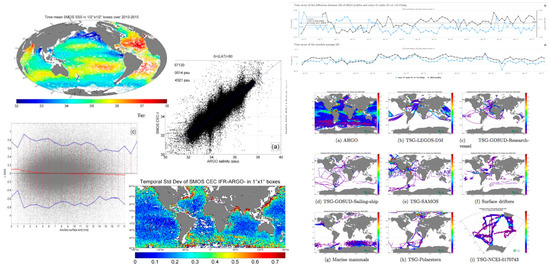
Figure 4.
Pictorial chart assembling some of the various metrics reported in the PI-MEP platform, ranging from temporal mean and dispersion of the salinity fields to scatter plots vs. in-situ data. Variation of salinity data are portrayed with respect to a variety of geophysical parameters (e.g., SST and WS), along with the numerous in-situ data considered in the dedicated match-up reports.
Numerous validation efforts estimated performance metrics for satellite salinity, such as, for instance, ref. [28]. The PI-MEP platform allows us to explore a wide range of geophysical and geographical conditions for an ample set of satellite and in-situ data, obtaining therefore a wide range of validation metrics. As a reference, multi-mission L4 product metrics are described in [31], where it is stated that over the global ocean, when considering all monthly matchups with Argo SSS, a robust STDD of 0.16 pss is obtained.
As of 2019, PI-MEP became an interagency ESA-NASA effort addressing validation and coordinated research and development on specific topics such as enhanced match-up criteria, triple-collocation analyses, and representation error characterization [32].
Over the last years, the Pi-MEP platform was not only serving the scope of versioning the various releases of SMOS L2OS processors and of ESA Climate Change Initiative (CCI) salinity (described afterwards), but also became the benchmark for assessing the entity of representation errors in satellite salinity measurements. Representation errors are the intrinsic sampling differences that emerge when comparing box-average satellite data with punctual in-space and in-time in-situ measurements. It may appear as sub-footprint variability or vertical stratification [33] for the spatial component and temporal aliasing for the time component. Within the Platform, these errors are being assessed through a variety of techniques, including high-resolution model sampling and Triple-Collocation analyses. These errors need to be properly quantified to distinguish the actual satellite inaccuracies from the inherent differences due to the sampling strategies and criteria.
Lastly, very recently, efforts for performing spectral analyses along TSG lines to estimate the effective resolution of all satellite products have been undertaken.
1.6. Additional Operational Production Chains
Only regarding the ocean products—since similar efforts are devoted to Soil Moisture, the hydrology counterpart measured by these L-band sensors—there is ample variety of products being generated globally. In Europe, besides the official ESA processing chain generating Level-2 (L2) Ocean Salinity products, two other distribution centers have been in charge of releasing Level-3 (L3) and Level-4 (L4) enhanced salinity products.
The Centre Aval de Traitement des Données SMOS (CATDS), out of France, is currently distributing a wealth of L2, L3, and L4 products, both operational and experimental, taking into account different algorithmic strategies. More specifically, the current CATDS portfolio embodies L2 (daily) and L3 (weekly-to-monthly) products, with a specific set of corrections on land-sea contamination and seasonal latitudinal biases, rain freshening correction, with different grid sampling and optimal interpolation techniques. More details can be found in [34], while the schematic in Figure 5 illustrates the typology and features of the various clusters of products served at CATDS.
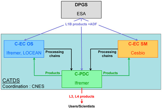
Figure 5.
Schematic flowchart of the various CATDS processing lines.
The Barcelona Expert Centre (BEC), out of Spain, has also been distributing for a long time an L2-to-L4 data stream by using a different inversion scheme, the so-called Debiased non-Bayesian (DnB) technique, which uses a different selection, statistical treatment, and filtering approach of the TBs and resulting SSS [35]. On top of these algorithmic strategies, the BEC processing chain also embodies different methodologies at L1, such as the Nodal Sampling technique to obtain a reliable set of TBs before the salinity retrieval procedure. Besides producing a global L3 and L4 product, BEC is also focusing on dedicated quasi-operational datasets on various basins (Arctic, Southern Ocean, Baltic, Black Sea, Mediterranean) with tailored processing adapted to the regional features and constraints (e.g., customized debiasing, temporal correction, land and ice contamination correction, etc.). More details can be found in Section 2.3.3 and in [36].
1.7. Climate Data Records
Within the umbrella of the ESA Climate Change Initiative—CCI, the Salinity_cci project started in 2015 with the aim of merging SMOS, SMAP, and Aquarius datasets and generating a consistent, coherent, long-term Climate Data Record (CDR), paving the way for climatic studies using salinity data from space. A specific approach adopted in merging the various satellite salinity sources is to retain the high variability sampled by the satellites, and specifically a temporal Optimal Interpolation (OI) approach is chosen to avoid any spatial smoothing of satellite SSS.
The v3 of the data record embedded a novel dielectric constant model and the usage of a more stable source of auxiliary data, coming from the ECMWF Reanalysis v5 (ERA-5), for SST and wind speed. The current version, v4 (shown as a sample for July 2022 in Figure 6), was extending further the dataset duration and improving performance in challenging ocean basins/regimes. CCI salinity fields are well-suited for monitoring weekly to interannual signals at spatial scales ranging from 50 km to the basin scale. A full summary of the algorithms adopted, the inherent validation (also using Pi-MEP salinity), and the derived scientific studies can be found in [31]. A dedicated effort for the production of a better high-latitude product is underway, and for the imminent v5, a stricter assessment of RFI is foreseen along with a better characterization of latitudinal correction.
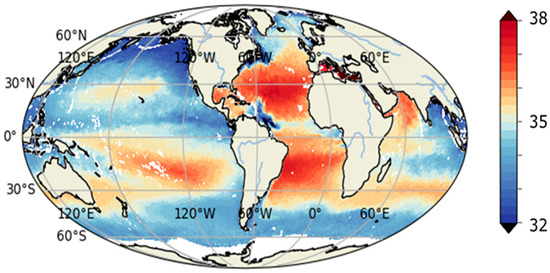
Figure 6.
CCI Salinity v4.0 L4 product corresponding to July 2022, out of the merging of SMOS/Aquarius/SMAP data.
Moreover, recent efforts are aimed at extending backward the Salinity CDR by using the ratio between C-band and X-band data from AMSR-E (and Windsat, in the near future) in specific conditions of warm waters and high salinity gradient, i.e., in major tropical river plumes. This is expected to be served as a research product in the CCI salinity CDR.
On the US side, a composite product referred to as OI-SSS is currently produced by Earth and Space Research (ESR), which currently embodies all three satellites in a specific Optimal Interpolation scheme. Namely, the two-month overlap (April–June 2015) between Aquarius and SMAP was used to ensure consistency in the data record. In-situ salinity from Argo floats and moored buoys is used to derive a large-scale bias correction for the entire OI-SSS dataset [37].
2. Research Advances in the Last Decade
The overwhelming collection of results gathered in the last decade, from the launch of the first salinity satellite to date, can be listed and summarized through several angles and clustered in different and even arbitrary ways. Unavoidably, some of the studies could be classified differently or would be overlapping two or more of these domain clusters. Here below, a non-exhaustive mapping of the various efforts is conveniently divided into three main categories, also following the areas identified in the latest SMOS extension review by an independent scientific panel, as
- Climate Applications,
- Science Applications, and
- Operational Applications.
The ocean salinity community is gathering on a fairly regular basis (about every 2 years) in a dedicated “Ocean Salinity Conference” to discuss and take stock of the various scientific, technological, and policy advancements in this domain. Besides, the fifth edition of the decadal “Oceans from Space” conference was also a crucial benchmark to gather the various achievements in several domains, ranging from ocean water cycle linkages to climate prediction. In this paper, the angle chosen is a different splitting of the activities with some updated results, the emphasis on specific efforts such as Pi-MEP Salinity, and updated discussions/feedback gathered at these thematic conferences.
For more in-depth discussion, a number of review papers [38,39,40] have already been published to give a detailed view of the various results obtained. An original schematic of the various applications addressed from space is given in the word cloud below (Figure 7).
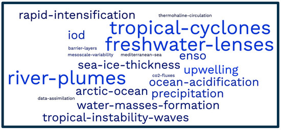
Figure 7.
Schematic of the various applications addressed from space. The bigger the size of the word, the more prominent is the attention dedicated to that specific topic. This chart is conceived by the authors and is obtained by using an online word-cloud generator.
2.1. Climate Applications
Over the last decade, SSS fingerprints have been progressively used in climate-related studies. An important aspect that has been elucidated is the relevance of satellite SSS in describing El Niño Southern Oscillations (ENSO) phases, such as the case of extension and contraction of the Pacific freshwater pool in accordance with El Niño and La Niña phases by using SMOS [41] or the ENSO-related displacement of salinity fronts by using Aquarius [42].
Salinity fingerprints related to other climate indices have been studied in the Indian Ocean Dipole (IOD) [43,44] and in relation to the North Atlantic Oscillation (NAO) [45]. Another phenomenon that has been monitored also through the use of spaceborne salinity is the evolution of Tropical Instability Waves (TIW), their speed, and their phasing with ENSO events, with both Aquarius [46] and CCI-Salinity data [47]. SMAP and SMOS SSS have also elucidated that monsoonal rain and runoff in the Indonesian Seas can substantially weaken the upper-layer transport of the Indonesian Throughflow, with significant impact on the transport of heat and other oceanic properties between the Pacific and Indian Oceans [48].
Additionally, the production of a salinity CDR, such as CCI-SSS, is also favoring updated studies on performance metrics. For instance, in [49] it is underlined how, using a high-resolution model reanalysis, most of the largest spatial variability of the satellite-minus-Argo salinity is observed in regions with large sampling mismatches. The authors underline how in dynamic areas (e.g., the Gulf Stream), the sampling mismatch between CCI-SSS and Argo can account for up to about 30% of the Root Mean Square Difference (RMSD).
Regarding climate trends, in [50] it was assessed how salinity trend estimates are influenced by decadal and longer-term salinity variability, while others [51] assessed multi-sensor satellite products in the Mediterranean Sea. Even if the time series is relatively short, a clear interannual trend is found on the Eastern side of the basin, leading to a marked salinification.
2.2. Science Applications
2.2.1. The Freshwater Domain
Major emphasis in the last decade has been devoted to the role of salinity as a tracer for freshwater fluxes. A plethora of studies and applications emerged thanks to the provision of consistent and accurate datasets of salinity from space, as partially described afterwards. A first aspect that has been studied has been the monitoring of major river basins and the assessment of the evolution of their freshwater plumes [52]. This is also one of the process studies consistently monitored in the Pi-MEP platform, which portrays the seasonal/inter-annual variability in the discharge and advection of freshwater plumes into the ocean. Through salinity, the freshwater plumes—and their direct effect on ocean circulation and gas exchanges—have been better characterized; thanks to the more frequent sampling induced by satellites [53].
Another set of studies [54,55,56] aimed at elucidating the occurrence of freshwater lenses on the ocean surface by combining salinity datasets and rain rate information (Figure 8). This had a twofold goal: On the one hand, to remove the impact of rain-induced freshening on the validation, and on the other hand, to use salinity as a proxy for studying the fate and dissipation of rain events. Modeling studies also helped in disentangling the rain-induced freshening from, e.g., advection of freshwater from other sources or locations [57].
Figure 8.
Excerpt of a salinity map elucidating various regimes in specific regions. Here, the meandering low-salinity signal associated with precipitation in the ITCZ is clearly depicted. Relevant regions are: (1) Amazon river plume; (2) Evaporation gyre; (3) Gulf Stream; (4) ITCZ; (5) Upwelling region.
Low surface salinity due to sea ice melting has been investigated by [58]; they found that meltwater lenses may persist more than a month and reach a surface salinity 5 pss fresher than surrounding waters. These studies were also benefiting from dedicated in-situ measurements collected in the uppermost skin layer by instrumentations such as the Salinity Snake, the Sea Surface Scanner (S3), and several drifters [59,60,61]. SSS as measured from satellites has also been merged with in situ data from profilers to obtain a 3D representation of the spatial and temporal evolution of freshwater pools, as described by [62]. Within the same framework of freshwater fluxes, but with emphasis on the evaporation regimes (which was also the focus of the SPURS-1 field experiment), the location and displacements of the salinity maxima in the various evaporation-dominated ocean gyres have been studied [63].
More generally, the balance of Evaporation–Precipitation (E-P) and its resemblance to salinity patterns has been widely studied by incorporating remotely sensed SSS [64], with special emphasis also on the areas that do not comply with the rain gauge approximation [65] and for which salinity represents the aggregate interplay of a wider set of phenomena (e.g., advection). In an even broader sense, salinity has been used to gather information on water cycle rates, gathering information on Pattern Amplification (PA) under the “rich gets richer” paradigm (causing, for instance, an enhancement of the inter-basin salinity difference) [66].
Additionally, both the pre-conditioning of and the a posteriori impacts of salinity on the passage of Tropical Cyclones (TC) and Extratropical Cyclones (ETC) have been widely assessed in the last ten years. Firstly, it was noted [67] that brightness temperatures, as measured by the available L-band satellite sensors, were sensitive to wind speed even in its severe regimes, unlike other sensors that experienced saturation and perturbation of additional noise sources (e.g., rain). This allowed the derivation of specific Geophysical Model Functions (GMF) that enabled retrieval of very high wind speed in hurricane conditions—recently complemented by Synthetic Aperture Radar (SAR) measurements to gain spatial resolution. Severe winds and Wind Radii products have been available since August 2021 in Near Real Time (within 4–6 h from acquisition) from the Institut Français de Recherche pour l’Exploitation de la Mer (IFREMER) and ESA. In relation to this, low salinity fields denoting stratified barrier layers were shown to be related to the so-called Rapid Intensification of a number of hurricanes in certain geophysical and geographical conditions. This has been shown to be due to the blocking effect of the barrier layer that hampered mixing with colder waters, which conventionally decreases the hurricane’s intensity. Lastly, satellite SSS also revealed haline hurricane wakes [68].
2.2.2. The Buoyancy Domain
In this Section, the various studies that relate to the implications of density changes due to salinity variability are described. Several studies looked at the phenomenon of stratification. Importantly, it has been pointed out [69] that, thanks to satellite estimations that are sensing the uppermost layer of the ocean, it is possible to describe an increased stratification of the surface layer if compared to the sub-surface layer conventionally sensed by the in situ measurements (Figure 9). As such, satellite-derived SSS measurements evidence an intensification of the water cycle (the freshest waters become even fresher and vice versa). A related set of studies paid attention to the barrier/slippery layers through investigation of the salinity surface patterns, for instance [70].
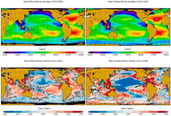
Figure 9.
Salinity maps and computed trends for the surface and near-surface layers, evidencing an increased stratification of the uppermost layer sensed from space. Reprinted/adapted with permission from Ref. [69]. Copyright year 2022, copyright owner is Olmedo, E.
The role of salinity in the context of seawater density has been inspected as well [71], paying attention specifically to density-compensation regimes and density ratio. This is especially relevant in the high latitudes, where density is almost completely controlled by salinity. Furthermore, and still within the buoyancy domain, surface Temperature/Salinity (T/S) diagrams have been estimated from space [72], and these have then been used as a diagnostic means to identify density fluxes and water mass formation areas and their geographic extent [73]. This latter approach has then been enhanced to include only satellite-based inputs in the derivation of Water Masses (WM) features of Transformation and Formation [74] and infer estimates of their variability and evolution.
Lastly, another fundamental oceanic process that benefited from the availability of satellite SSS is the characterization of upwelling. For instance, exchanges of salt between the deep ocean and the surface provided additional constraints in the description of upwelling events [75,76].
2.2.3. The Bio-Geo-Chemistry Domain
A relatively novel application framework has been the biogeochemical domain. While applications and usage of satellite salinity in the physical oceanography context were natural, its perusal with the wider biogeochemistry realm was not to be taken for granted. First studies, a few years after the launch of satellite sensors, aimed at estimating pCO2 also through salinity parameterizations [77]. In parallel, and for the following years, the relationship between salinity and Coloured Dissolved Organic Matter (CDOM) at major river mouths has been used to estimate salinity in the proximity of the coasts that are subject to freshwater runoff dispersal [78]. Later on, the strong relationship between salinity and alkalinity (the buffer capacity of the ocean to neutralize acids) has been exploited [79], eventually estimating the full marine carbonate system, including the surface ocean pH [80]. Eventually, these estimates have also been used for the monitoring of CO2 fluxes and their current crucial implications as per carbon sequestration and inventory, widening even more the range of applications that emerged by the consistent use of satellite SSS.
2.3. Operational Applications
2.3.1. Data Assimilation
Although in the first years remotely sensed salinity estimates from space suffered from some inertia in their applications within the wider operational community, the increasingly accurate and debiased fields produced from SMOS, Aquarius, and SMAP fostered their use in several Data Assimilation (DA) experiments to constrain ocean state estimation and to initialize ocean and climate predictions. Most notably, regarding SMOS, a first experiment was undertaken by Mercator Ocean in the late 2010s, which showed how the introduction of SSS in their ocean model would be neutral-to-beneficial in the description of the various ocean state variables [81]. This was followed by a similar exercise at the UK Met Office [82]. Both efforts are now being repeated with a more updated merged version of salinity fields coming from CCI. The University of Hamburg, Germany, was also involved in DA and comparison exercises focusing on the seasonal to interannual variability of salinity as underlined by satellites and model intercomparison [83]. On the US side, a set of experiments have been carried out at both NASA and the National Oceanic and Atmospheric Administration (NOAA) with the aim of assessing the potential of satellite SSS to improve El Niño Southern Oscillations (ENSO) predictions [84,85].
In terms of operational data provision, the Copernicus Marine Service, or in full the Copernicus Marine Environment Monitoring Service (CMEMS), delivers a multi-observation global gap-free L4 analysis of Sea Surface Salinity (SSS) that has been obtained through a multivariate optimal interpolation algorithm that combines SMOS satellite estimates and in situ salinity measurements with satellite SST information [86]. Recently, a purely satellite-based product derived from CATDS is also being served.
As mentioned in the previous Section, the R&D efforts in estimating WS parameters in gale-force regimes became operational (Figure 10), and the output products (especially wind radii) are in turn ingested by a variety of Tropical Cyclone Forecast Centers (e.g., US Naval Research Laboratory, NOAA, Meteo-France) to generate warnings and issue evacuation alerts over hazardous areas.
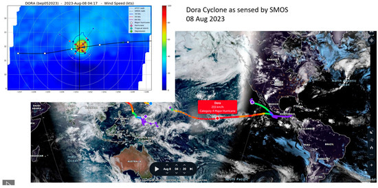
Figure 10.
Trajectory, intensity and the evolution of the Cyclone Dora, as sensed operationally by SMOS in August 2023 (Credits: N. Reul, IFREMER).
2.3.2. Prognostic
A very interesting focus was portrayed by colleagues at Woods Hole Oceanographic Institution (WHOI) that studied the potential role of salinity as a prognostic variable to identify potential landfall over continental areas. Specifically, a study [87] assessed characteristics of the salinity fields and temporal lags with an atmospheric model to elucidate the transport of evaporated moisture and subsequent intense precipitation over the US Midwest. This has also been studied in the context of Neural Network (NN) schemes with additional ocean variables to forecast rain events [88].
2.3.3. Dedicated Regional Datasets
Estimations of SSS in regional and/or semi-enclosed basins, or at high latitudes, have always been challenging due to an interplay of their geophysical and geographical connotations and constraints. Specifically, salinity retrieval at high latitudes characterized by low SST and usually high winds has always been difficult due to the decreased sensitivity of TB to SSS in cold waters, enhanced by the difficulty of characterizing the roughness effect at high winds. Additionally, both the relatively coarse spatial resolution that limits the vicinity to coasts and also the presence of land that introduces a disturbance signal leakage hamper reliable retrievals in semi-enclosed basins. Recently, novel retrieval methodologies and data filtering ensured promising results and the generation of quasi-operational bespoke datasets at high latitudes (Arctic, Southern Ocean) [89,90] and also in the Mediterranean regions [91], as well as the Baltic Sea and Black Sea [92,93]. The dedicated Arctic Salinity product has also been ingested in the Copernicus Arctic Ice-Ocean reanalysis TOPAZ4 system [94]. Recently, CATDS also produced a dedicated set of regional products in 8 different regions [95].
3. Missions in the Upcoming Decade
3.1. Short-Term Developments of Ongoing Missions
Although Aquarius was lost in 2015, as of 2024, both SMOS and SMAP are still operational, exceeding by far their nominal expected lifetime. As such, both missions are still subject to ongoing improvements on several aspects, ranging from the algorithm developments to error characterization and from auxiliary data handling to the minimization of related perturbation sources. A large variety of L3 and L4 products stemming from additional processing of these satellite data streams, including merging among these sources and also with in-situ data, are available and collated in the Pi-MEP salinity platform as described above.
In spite of the remarkable advancements described above on a broad variety of oceanographic and climatic topics, discussions on limitations, shortcomings, current concerns, and possible ways forward are still debated and brainstormed in general meetings such as “Oceans from Space”. Satellite SSS continuity in itself remains the major objective and desire, given that the generated CDRs necessarily build on long and stable datasets in order to produce relevant climate analyses. For instance, in the near future, attempts will be made to merge the various satellite TBs at L1, homogenizing thus the usage of dielectric constant models and auxiliary data. This is even more relevant, since upcoming missions focused on or including L-band will be available some time in the future (see below), and therefore, ensuring no gaps will be crucial.
Another aspect of the quest for continuity is the preservation of the set-aside passive L-band that is severely threatened by competing interests in the area of mobile telecommunications; under the motto “use it or lose it”, the community is advocating for the maintenance of this band and indeed for enforcing regulations to diminish and switch off harmful RFI sources. On the geophysical aspects, conventional concerns in the community are still the improvement of accuracy and spatial resolution, especially for polar oceans and coastal regions, which are evidently paramount areas of interest per their relevance to climate and human activities.
Aiming at addressing scientific gaps and further improving the current estimates, several technological developments and satellite designs have been proposed over the years, with various feasibility studies funded by several space Agencies. At the recent ESA call for Earth Explorer-12 (EE-12), three proposals included L-band sensors with very different designs to estimate salinity from space at various spatial and temporal resolutions. One of them has been retained for further assessment in the initial Phase-0 (CryoRad) [96], which will use an innovative low-frequency wideband radiometer that includes SSS estimations among its primary objectives (Figure 11). The two other proposals, namely the Fine Resolution Explorer for Salinity, Carbon, and Hydrology (FReSCH) and the Sea-Air-Ice-Land Interactions (SAILIN), are under discussion in the community to further explore the innovative technological and development elements that were proposed (although not selected), both aiming at using innovative interferometric concepts to reach a desirable 10 km spatial resolution.
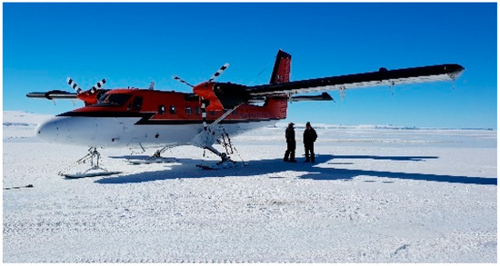
Figure 11.
Preliminary field experiments to assess the capability of the wideband radiometer proposed for the EE-12 candidate CryoRad mission.
3.2. The CIMR Mission: Rationale and Multifrequency Capabilities
Aside from the R&D line of the ESA Earth Explorers, in the framework of Copernicus Expansion and within the context of the High Priority Candidate Missions (HPCM), the Copernicus Imaging Microwave Radiometer (CIMR) has been selected for Phase B/C/D after successfully passing a Preliminary Design Review and towards a full Critical Design Review to be held in 2026.
The Copernicus Imaging Microwave Radiometer (CIMR) aims at addressing user requirements as specified by the EC Polar Expert Group (PEG) in its related set of reports. CIMR is a wide-swath imager with multi-frequency and multi-spectral capability geared towards operational monitoring. Major technical features are a conical scanning (Forward scan and Aft scan) with a Sun-synchronous dawn-dusk orbit, with a sub-daily revisit and full Arctic coverage (Figure 12). The multi-frequency capability is represented by the selection of 6 channels at L-, C-, X-, K-, and Ka-band, with L-band intended to give continuity to SMOS and SMAP measurements. All channels have an onboard RFI processor to identify interference and remove it from the measurement.
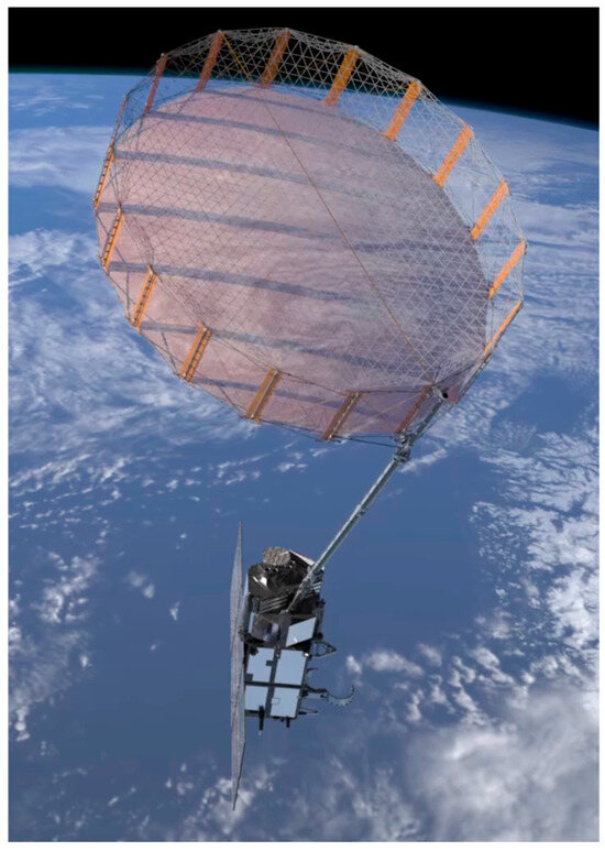
Figure 12.
Artistic view of the CIMR satellite.
As noted, CIMR will include an L-band channel, which will allow estimates of ocean salinity with high revisit time and with collocated measurements of SST and WS, which will aid accurate salinity retrieval in the challenging ocean regions at high latitudes. Primary geophysical variables over the ocean are Sea-Ice Concentration (SIC), thin Sea-Ice Thickness (SIT), SST, SSS, ice sheet, Sea Level change, and Wind Speed [97]. Two satellites are meant to be flown sequentially with an overlap. The expected launch of the first satellite is for 2029.
4. Conclusions
After a couple of decades of technology development and applications for funding, the panorama of salinity-enabled oceanographic and climatic studies radically changed with the advent of SMOS in 2009, which provided the first-ever satellite measurement of SSS. SMOS was followed by Aquarius in 2011 and SMAP in 2015 to create a stream of continuous and increasingly accurate estimates of SSS from space.
SMOS, being the first-ever measurement with a disruptive novel technology (synthetic aperture radiometry), was inherently prone to technical and scientific challenges. With the experience acquired over a decade and via the cross-fertilization of competences among the various sensor communities, many of these shortcomings have been addressed or drastically reduced (RFI, Land-Sea Contamination, and external noise source handling).
Both the current versions of the still-operational sensors (SMOS v700 and SMAP v5) represent a solid and stable dataset to enable science and applications. Novel consolidated platforms (Pi-MEP Salinity) ensure enhanced validation and stimulate oceanographic process studies by embedding a broad set of salinity products from space, altogether with model outputs and a remarkable variety of in-situ ground data, with corresponding match-up reports. Sustained focus over the last years was on the generation of merged salinity products, which establish specific Climate Data Records, most notably CCI-Salinity.
By progressively tackling all the processing issues and improving satellite accuracies, a wide range of oceanographic applications using spaceborne SSS developed (air-sea interactions, ocean circulation and modeling, climate indexes monitoring, marine biogeochemistry, Numerical Weather Prediction, etc.), and they are further enlarging with the release of the latest salinity reprocessing. The planned CIMR mission will perpetuate community expertise in L-band radiometry science, development, and operations, with a distinct focus on high latitudes.
Author Contributions
Writing—original draft preparation, R.S.; writing—review and editing, J.B., N.R. and T.L.; supervision and validation, S.H.Y. All authors have read and agreed to the published version of the manuscript.
Funding
This research received no external funding.
Data Availability Statement
No new data were created or analyzed in this study. Data sharing is not applicable to this article.
Acknowledgments
The authors acknowledge two anonymous reviewers for their constructive remarks that improved the clarity and structure of the paper. The following list of scientists, engineers, and managers involved in the oceanic branch of the Ocean Salinity missions, albeit non-exhaustive, is compiled here below to acknowledge their invaluable contributions to the missions success: J. Font, J. Tenerelli, A. Turiel, J.-L. Vergely, E. Olmedo, E. Lindstrom, N. Vinogradova, G. Lagerloef, J. Schanze, F. Bingham, D. Levine, Y. Kerr, P. Spurgeon, M. Arias, F. D’Amico, R. Catany, E. Jeansou, Y. Rey-Ricord, R. Oliva, S. Guimbard, C. Gabarrò, J. Martinez, V. Gonzalez, C. Gonzalez, A. Garcia, M. Talone, D. Khvorostyanov, A. Parracho, S. Tarot, D. Stammer, M. Senna-Martins, S. Brown, S. Misra, E. Dinnat, A. Camps, F. Bonjean, A. Martin, N. Kolodziejczyk, G. Reverdin, F. Rouffi, J. Jouanno, C. Maes, X. Yin, A. Hasson, A. Supply, F. Gaillard, C. Thouvenin-Masson, N. Martin, G. Alory, A. Gordon, R. Schmitt, T. Meissner, L. Yu, S. Fournier, E. Hackert, L. Li, O. Melnichenko, E. Bayler; K. Druschka, J. Anderson, W.L., Asher, B. Subrahmanyam, B. Ward, W. Tang, S. Grodsky, B. Chapron, B. Buongiorno Nardelli, L. Bertino, A. Soloviev, K. Scipal, S. Mecklenburg, M. Drusch, R. Crapolicchio, R. Diez, M. Martin-Neira, A. de la Fuente, J. Fauste, D. Fernandez, P. Cipollini, C. Donlon, S. Delwart, M. Drinkwater, A. Hahne.
Conflicts of Interest
The authors declare no conflicts of interest.
References
- Barale, V. Half-a-Century of Oceans from Space: Features & Futures. Remote Sens. 2023, 15, 4064. [Google Scholar] [CrossRef]
- Barale, V.; Gower, J.F.R.; Alberotanza, L. (Eds.) Oceans from Space, Venice 2000, Abstracts; EUR 19661 EN; Publication Office of the European Union: Luxemburg, 2010; p. 282. Available online: https://publications.jrc.ec.europa.eu/repository/handle/JRC20666 (accessed on 19 June 2025).
- Lagerloef, G.; Font, J. SMOS and Aquarius/SAC-D Missions: The Era of Space Borne Salinity Measurements is About to Begin. In Oceanography from Space, Revisited; Barale, V., Gower, J.F.R., Alberotanza, L., Eds.; Springer: Dordrecht, The Netherlands; Heidelberg, Germany; London, UK; New York, NY, USA, 2010; pp. 35–58. [Google Scholar] [CrossRef]
- Barale, V.; Gower, J.F.R.; Alberotanza, L. (Eds.) Proceedings “Oceans from Space” V, Venice 2022; NSA GROUP: Roma, Italy, 2022; p. 252. [Google Scholar] [CrossRef]
- Durack, P.J. Ocean salinity and the global water cycle. Oceanography 2015, 28, 20–31. [Google Scholar] [CrossRef]
- Roemmich, D.; Gilson, J. The 2004–2008 mean and annual cycle of temperature, salinity, and steric height in the global ocean from the Argo Program. Prog. Oceanogr. 2009, 82, 81–100. [Google Scholar] [CrossRef]
- Kerr, Y.H.; Waldteufel, P.; Wigneron, J.P.; Delwart, S.; Cabot, F.; Boutin, J.; Escorihuela, M.J.; Font, J.; Reul, N.; Gruhier, C.; et al. The SMOS Mission: New Tool for Monitoring Key Elements of the Global Water Cycle. Proc. IEEE 2010, 98, 666–687. [Google Scholar] [CrossRef]
- Suess, M.; Matos, P.; Gutierrez, A.; Zundo, M.; Martín-Neira, M. Processing of SMOS level 1C data onto a discrete global grid. In Proceedings of the 2004 IEEE International Geoscience and Remote Sensing Symposium (IGARSS 2004), Anchorage, AK, USA, 20–24 September 2004; Volume 3, pp. 1914–1917. [Google Scholar]
- Daganzo-Eusebio, E.; Oliva, R.; Kerr, Y.H.; Nieto, S.; Richaume, P.; Mecklenburg, S.M. SMOS Radiometer in the 1400–1427-MHz Passive Band: Impact of the RFI Environment and Approach to Its Mitigation and Cancellation. IEEE Trans. Geosci. Remote Sens. 2013, 51, 4999–5007. [Google Scholar] [CrossRef]
- Boutin, J.; Martin, N.; Yin, X.; Font, J.; Reul, N.; Spurgeon, P. First Assessment of SMOS Data Over Open Ocean: Part II—Sea Surface Salinity. IEEE Trans. Geosci. Remote Sens. 2012, 50, 1662–1675. [Google Scholar] [CrossRef]
- Yueh, S.H.; Chaubell, J. Sea surface salinity and wind retrieval using combined passive and active L-band microwave observations. IEEE Trans. Geosci. Remote Sens. 2011, 50, 1022–1032. [Google Scholar] [CrossRef]
- Reul, N.; Fournier, S.; Boutin, J.; Hernandez, O.; Maes, C.; Chapron, B.; Alory, G.; Quilfen, Y.; Tenerelli, J.; Morisset, S.; et al. Sea Surface Salinity Observations from Space with the SMOS Satellite: A New Means to Monitor the Marine Branch of the Water Cycle. Surv. Geophys. 2014, 35, 681–722. [Google Scholar] [CrossRef]
- Boutin, J.; Vergely, J.-L.; Dinnat, E.P.; Waldteufel, P.; D’Amico, F.; Reul, N.; Supply, A.; Thouvenin-Masson, C. Correcting sea surface temperature spurious effects in salinity retrieved from spaceborne L-band radiometer measurements. IEEE Trans. Geosci. Remote Sens. 2021, 59, 7256–7269. [Google Scholar] [CrossRef]
- Yin, X.; Boutin, J.; Dinnat, E.; Song, Q.; Martin, A. Roughness and foam signature on SMOS-MIRAS brightness temperatures: A semi-theoretical approach. Remote Sens. Environ. 2016, 180, 221–233. [Google Scholar] [CrossRef]
- Spurgeon, P.; Font, J.; Boutin, J.; Reul, N.; Tenerelli, J.; Vergely, J.L.; Gabarro, C.; Yin, X.; Lavender, S.; Chuprin, A.; et al. Ocean salinity retrieval approaches for the SMOS satellite. In Proceedings of the ESA Living Planet Symposium, Bergen, Norway, 28 June–2 July 2010. [Google Scholar]
- Martín-Neira, M.; Oliva, R.; Corbella, I.; Torres, F.; Duffo, N.; Durán, I.; Kainulainen, J.; Closa, J.; Zurita, A.; Cabot, F.; et al. Lessons learnt from SMOS after 7 years in orbit. In Proceedings of the 2017 IEEE International Geoscience and Remote Sensing Symposium (IGARSS), Fort Worth, TX, USA, 23–28 July 2017; pp. 255–258. [Google Scholar]
- Font, J.; Camps, A.; Borges, A.; Martín-Neira, M.; Boutin, J.; Reul, N.; Kerr, Y.H.; Hahne, A.; Mecklenburg, S. SMOS: The challenging sea surface salinity measurement from space. Proc. IEEE 2009, 98, 649–665. [Google Scholar] [CrossRef]
- Lagerloef, G.; Colomb, F.R.; Le Vine, D.; Wentz, F.; Yueh, S.; Ruf, C.; Lilly, J.; Gunn, J.; Chao, Y.; de Charon, A.; et al. The Aquarius/SAC-D mission—Designed to meet the salinity remote sensing challenge. Oceanogr. Mag. 2008, 21, 68–81. [Google Scholar] [CrossRef]
- Le Vine, D.M.; Matthaeis, P.d. Aquarius active/passive RFI environment at L-band. IEEE Geosci. Remote Sens. Lett. 2014, 11, 1747–1751. [Google Scholar] [CrossRef]
- Entekhabi, D.; Njoku, E.G.; O’Neill, P.E.; Kellogg, K.H.; Crow, W.T.; Edelstein, W.N.; Entin, J.K.; Goodman, S.D.; Jackson, T.J.; Johnson, J.; et al. The soil moisture active passive (SMAP) mission. Proc. IEEE 2010, 98, 704–716. [Google Scholar] [CrossRef]
- Piepmeier, J.R.; Focardi, P.; Horgan, K.A.; Knuble, J.; Ehsan, N.; Lucey, J.; Brambora, C.; Brown, P.R.; Hoffman, P.J.; French, R.T.; et al. SMAP L-Band Microwave Radiometer: Instrument Design and First Year on Orbit. IEEE Trans. Geosci. Remote Sens. 2017, 55, 1954–1966. [Google Scholar] [CrossRef]
- Mohammed, P.N.; Aksoy, M.; Piepmeier, J.R.; Johnson, J.T.; Bringer, A. SMAP L-band microwave radiometer: RFI mitigation prelaunch analysis and first year on-orbit observations. IEEE Trans. Geosci. Remote Sens. 2016, 54, 6035–6047. [Google Scholar] [CrossRef]
- Olmedo, E.; Martínez, J.; Turiel, A.; Ballabrera-Poy, J.; Portabella, M. Debiased non-Bayesian retrieval: A novel approach to SMOS sea surface salinity. Remote Sens. Environ. 2017, 193, 103–126. [Google Scholar] [CrossRef]
- Mecklenburg, S.; Drusch, M.; Kaleschke, L.; Rodriguez-Fernandez, N.; Reul, N.; Kerr, Y.; Font, J.; Martin-Neira, M.; Oliva, R.; Daganzo-Eusebio, E.; et al. ESA’s Soil Moisture and Ocean Salinity mission: From science to operational applications. Remote Sens. Environ. 2016, 180, 3–18. [Google Scholar] [CrossRef]
- Lindstrom, E.J.; Bryan, F.; Schmitt, R. SPURS: Salinity processes in the upper-ocean regional study—The North Atlantic experiment. Oceanography 2015, 28, 14–19. [Google Scholar] [CrossRef]
- Lindstrom, E.J.; Edson, J.B.; Schanze, J.J.; Shcherbin, A.Y. SPURS-2: Salinity processes in the upper-ocean regional study 2. The eastern equatorial Pacific experiment. Oceanography 2019, 32, 15–19. [Google Scholar] [CrossRef]
- Gordon, A.L.; Giulivi, C.F.; Busecke, J.; Bingham, F.M. Differences among subtropical surface salinity patterns. Oceanography 2015, 28, 32–39. [Google Scholar] [CrossRef]
- Hernandez, O.; Boutin, J.; Kolodziejczyk, N.; Reverdin, G.; Martin, N.; Gaillard, F.; Reul, N.; Vergely, J.L. SMOS salinity in the subtropical North Atlantic salinity maximum: 1. Comparison with Aquarius and in situ salinity. J. Geophys. Res. Ocean. 2014, 119, 8878–8896. [Google Scholar] [CrossRef]
- Drushka, K.; Westbrook, E.; Bingham, F.M.; Gaube, P.; Dickinson, S.; Fournier, S.; Menezes, V.; Misra, S.; Pérez Valentín, J.; Rainville, E.J.; et al. Salinity and Stratification at the Sea Ice Edge (SASSIE): An oceanographic field campaign in the Beaufort Sea. Earth Syst. Sci. Data 2024, 16, 4209–4242. [Google Scholar] [CrossRef]
- Guimbard, S.; Reul, N.; Sabia, R.; Herlédan, S.; Khoury Hanna, Z.E.; Piollé, J.F.; Paul, F.; Lee, T.; Schanze, J.J.; Bingham FMLe Vine, D. The salinity pilot-mission exploitation platform (Pi-mep): A hub for validation and exploitation of satellite sea surface salinity data. Remote Sens. 2021, 13, 4600. [Google Scholar] [CrossRef]
- Boutin, J.; Reul, N.; Koehler, J.; Martin, A.; Catany, R.; Guimbard, S.; Rouffi, F.; Vergely, J.L.; Arias, M.; Chakroun, M.; et al. Satellite-based sea surface salinity designed for ocean and climate studies. J. Geophys. Res. Ocean. 2021, 126, e2021JC017676. [Google Scholar] [CrossRef]
- Guimbard, S.; Reul, N.; Díez-García, R.; Herlédan, S.; El Khoury Hanna, Z.; Lee, T.; Schanze, J.; Bingham, F.; Scipal, K. Advancing Sea Surface Salinity R&D: The Pi-MEP Initiative for Satellite Salinity Data Validation and Exploitation. In Proceedings of the EGU General Assembly Conference Abstracts, Vienna, Austria, 14–19 April 2024; p. 12907. [Google Scholar]
- Boutin, J.; Chao, Y.; Asher, W.E.; Delcroix, T.; Drucker, R.; Drushka, K.; Kolodziejczyk, N.; Lee, T.; Reul, N.; Reverdin, G.; et al. Satellite and In Situ Salinity: Understanding Near-Surface Stratification and Subfootprint Variability. Bull. Am. Meteorol. Soc. 2016, 97, 1391–1407. [Google Scholar] [CrossRef]
- Tarot, S.; Boutin, J.; Kerr, Y.; Vergely, J.L.; Mialon, A.; Vandermarcq, O. CATDS: SMOS L3/L4 salinity products generation and dissemination. In Proceedings of the 7th Ocean Salinity Conference 2024, Noordwijk, The Netherlands, 13–16 May 2024. [Google Scholar]
- Hoareau, N.; Turiel, A.; Portabella, M.; Ballabrera-Poy JVogelzang, J. Singularity power spectra: A method to assess geophysical consistency of gridded products—Application to sea-surface salinity remote sensing maps. IEEE Trans. Geosci. Remote Sens. 2018, 56, 5525–5536. [Google Scholar] [CrossRef]
- Olmedo, E.; González-Haro, C.; Hoareau, N.; Umbert, M.; González-Gambau, V.; Martínez, J.; Gabarró, C.; Turiel, A. Nine years of SMOS sea surface salinity global maps at the Barcelona Expert Center. Earth Syst. Sci. Data Discuss. 2020, 2020, 1–49. [Google Scholar] [CrossRef]
- Melnichenko, O.; Hacker, P.; Potemra, J.; Meissner, T.; Wentz, F. A New Multi-Mission Sea Surface Salinity Optimum Interpolation (OISSS) Analysis for Ocean Research and Applications. In Proceedings of the EGU General Assembly Conference Abstracts, Vienna, Austria, 23–28 April 2023; p. EGU-3755. [Google Scholar]
- Vinogradova, N.; Lee, T.; Boutin, J.; Drushka, K.; Fournier, S.; Sabia, R.; Stammer, D.; Bayler, E.; Reul, N.; Gordon, A.; et al. Satellite Salinity Observing System: Recent Discoveries and the Way Forward. Front. Mar. Sci. 2019, 6, 243. [Google Scholar] [CrossRef]
- Reul, N.; Grodsky, S.A.; Arias, M.; Boutin, J.; Catany, R.; Chapron, B.; D’amico, F.; Dinnat, E.; Donlon, C.; Fore, A.; et al. Sea surface salinity estimates from spaceborne L-band radiometers: An overview of the first decade of observation (2010–2019). Remote Sens. Environ. 2020, 242, 111769. [Google Scholar]
- Boutin, J.; Yueh, S.; Bindlish, R.; Chan, S.; Entekhabi, D.; Kerr, Y.; Kolodziejczyk, N.; Lee, T.; Reul, N.; Zribi, M. Soil Moisture and Sea Surface Salinity Derived from Satellite-Borne Sensors. Surv. Geophys. 2023, 44, 1449–1487. [Google Scholar] [CrossRef]
- Hasson, A.; Delcroix, T.; Boutin, J.; Dussin, R.; Ballabrera-Poy, J. Analyzing the 2010–2011 La Niña signature in the tropical Pacific sea surface salinity using in situ data, SMOS observations, and a numerical simulation. J. Geophys. Res. Ocean. 2014, 119, 3855–3867. [Google Scholar] [CrossRef]
- Qu, T.; Yu, J.Y. ENSO indices from sea surface salinity observed by Aquarius and Argo. J. Oceanogr. 2014, 70, 367–375. [Google Scholar] [CrossRef]
- Akhil, V.P.; Vialard, J.; Lengaigne, M.; Keerthi, M.G.; Boutin, J.; Vergely, J.L.; Papa, F. Bay of Bengal Sea surface salinity variability using a decade of improved SMOS re-processing. Remote Sens. Environ. 2020, 248, 111964. [Google Scholar] [CrossRef]
- Du, Y.; Zhang, Y. Satellite and argo observed surface salinity variations in the tropical indian ocean and their association with the Indian Ocean dipole mode. J. Clim. 2015, 28, 695–713. [Google Scholar] [CrossRef]
- Da, N.D.; Foltz, G.R. Interannual variability and multiyear trends of sea surface salinity in the Amazon-Orinoco plume region from satellite observations and an ocean reanalysis. J. Geophys. Res. Ocean. 2022, 127, e2021JC018366. [Google Scholar] [CrossRef]
- Lee, T.; Lagerloef, G.; Gierach, M.M.; Kao, H.-Y.; Yueh, S.; Dohan, K. Aquarius reveals salinity structure of tropical instability waves. Geophys. Res. Lett. 2012, 39, L12610. [Google Scholar] [CrossRef]
- Olivier, L.; Reverdin, G.; Hasson, A.; Boutin, J. Tropical Instability Waves in the Atlantic Ocean: Investigating the Relative Role of Sea Surface Salinity and Temperature From 2010 to 2018. J. Geophys. Res. Ocean. 2020, 125, e2020JC016641. [Google Scholar] [CrossRef]
- Lee, T.; Fournier, S.; Gordon, A.L.; Sprintall, J. Maritime Continent water cycle regulates low-latitude chokepoint of global ocean circulation. Nat. Commun. 2019, 10, 2103. [Google Scholar] [CrossRef]
- Thouvenin-Masson, C.; Boutin, J.; Vergely, J.-L.; Reverdin, G.; Martin, A.C.H.; Guimbard, S.; Reul, N.; Sabia, R.; Catany, R.; Fanton-d’Andon, O.H. Satellite and In Situ Sampling Mismatches: Consequences for the Estimation of Satellite Sea Surface Salinity Uncertainties. Remote Sens. 2022, 14, 1878. [Google Scholar] [CrossRef]
- Stammer, D.; Martins, M.S.; Köhler, J.; Köhl, A. How well do we know ocean salinity and its changes? Prog. Oceanogr. 2021, 190, 102478. [Google Scholar] [CrossRef]
- Sammartino, M.; Aronica, S.; Santoleri, R.; Buongiorno Nardelli, B. Retrieving Mediterranean Sea surface salinity distribution and interannual trends from multi-sensor satellite and in situ data. Remote Sens. 2022, 14, 2502. [Google Scholar] [CrossRef]
- Fournier, S.; Lee, T.; Gierach, M.M. Seasonal and interannual variations of sea surface salinity associated with the Mississippi River plume observed by SMOS and Aquarius. Remote Sens. Environ. 2016, 180, 431–439. [Google Scholar] [CrossRef]
- Grodsky, S.A.; Reverdin, G.; Carton, J.A.; Coles, V.J. Year-to-Year Salinity Changes in the Amazon Plume: Contrasting 2011 and 2012 Aquarius/SAC-D and SMOS Satellite Data. Remote Sens. Environ. 2014, 140, 14–22. [Google Scholar] [CrossRef]
- Boutin, J.; Martin, N.; Reverdin, G.; Morisset, S.; Yin, X.; Centurioni, L.; Reul, N. Sea surface salinity under rain cells: SMOS satellite and in situ drifters observations, Journal of Geophysical Research. Oceans 2014, 119, 5533–5545. [Google Scholar]
- Supply, A.; Boutin, J.; Vergely, J.-L.; Martin, N.; Hasson, A.; Reverdin, G.; Mallet, C.; Viltard, N. Precipitation estimates from SMOS sea-surface salinity. Q. J. R. Meteorol. Soc. 2018, 144 (Suppl. S1), 103–119. [Google Scholar] [CrossRef]
- Drushka, K.; Asher, W.; Jessup, A.; Thompson, E.; Iyer, S.; Clark, D. Capturing fresh layers with the surface salinity profile. Oceanography 2019, 32, 76–85. [Google Scholar] [CrossRef]
- Santos-Garcia, A.; Jacob, M.M.; Jones, W.L.; Asher, W.E.; Hejazin, Y.; Ebrahimi, H.; Rabolli, M. Investigation of rain effects on Aquarius Sea Surface Salinity measurements. J. Geophys. Res. Ocean. 2014, 119, 7605–7624. [Google Scholar] [CrossRef]
- Supply, A.; Boutin, J.; Reverdin, G.; Vergely, J.-L.; Bellenger, H. Variability of Satellite Sea Surface Salinity Under Rainfall. In Satellite Precipitation Measurement: Volume 2; Levizzani, V., Kidd, C., Kirschbaum, D.B., Kummerow, C.D., Nakamura, K., Turk, F.J., Eds.; Springer International Publishing: Cham, Switzerland, 2020. [Google Scholar]
- Anderson, J.; Riser, S. Near-surface variability of temperature and salinity in the near-tropical ocean: Observations from profiling floats. J. Geophys. Res. Ocean. 2014, 119, 2169–9275. [Google Scholar] [CrossRef]
- Reverdin, G.; Morisset, S.; Boutin, J.; Martin, N.; Sena-Martins, M.; Gaillard, F.; Blouch, P.; Rolland, J.; Font, J.; Salvador, J.; et al. Validation of salinity data from surface drifters. J. Atmos. Ocean. Technol. 2014, 31, 967–983. [Google Scholar] [CrossRef]
- Ribas-Ribas, M.; Hamizah Mustaffa, N.I.; Rahlff, J.; Stolle, C.; Wurl, O. Sea surface scanner (s 3): A catamaran for high-resolution measurements of biogeochemical properties of the sea surface microlayer. J. Atmos. Ocean. Technol. 2017, 34, 1433–1448. [Google Scholar] [CrossRef]
- Guimbard, S.; Reul, N.; Chapron, B.; Umbert, M.; Maes, C. Seasonal and interannual variability of the Eastern Tropical Pacific Fresh Pool. J. Geophys. Res. Ocean. 2017, 122, 1749–1771. [Google Scholar] [CrossRef]
- Bingham, F.M.; Busecke, J.; Gordon, A.L.; Giulivi, C.F.; Li, Z. The North Atlantic subtropical surface salinity maximum as observed by Aquarius. J. Geophys. Res. Ocean. 2014, 119, 7741–7755. [Google Scholar] [CrossRef]
- Schanze, J.J.; Schmitt, R.W.; Yu, L.L. The global oceanic freshwater cycle: A state-of-the-art quantification. J. Mar. Res. 2010, 68, 569–595. [Google Scholar] [CrossRef]
- Yu, L. A global relationship between the ocean water cycle and near-surface salinity. J. Geophys. Res. 2011, 116, C10025. [Google Scholar] [CrossRef]
- Skliris, N.; Zika, J.D.; Nurser, G.; Josey, S.A.; Marsh, R. Global water cycle amplifying at less than the Clausius-Clapeyron rate. Sci. Rep. 2016, 6, 752. [Google Scholar] [CrossRef] [PubMed]
- Reul, N.; Chapron, B.; Zabolotskikh, E.; Donlon, C.; Quilfen, Y.; Guimbard, S.; Piolle, J.F. A revised L-band radio-brightness sensitivity to extreme winds under Tropical Cyclones: The five year SMOS-storm database. Remote Sens. Environ. 2016, 180, 274–291. [Google Scholar] [CrossRef]
- Grodsky, S.A.; Reul, N.; Lagerloef, G.; Reverdin, G.; Carton, J.A.; Chapron, B.; Quilfen, Y.; Kudryavtsev, V.N.; Kao, H.-Y. Haline hurricane wake in the Amazon/Orinoco plume: AQUARIUS/SACD and SMOS observations. Geophys. Res. Lett. 2012, 39, L20603. [Google Scholar] [CrossRef]
- Olmedo, E.; Turiel, A.; González-Gambau, V.; Gonzalez-Haro, C.; Garcia-Espriu, A.; Gabarrò, C.; Portabella, M.; Corbella, I.; Martin-Neira, M.; Arias, M.; et al. Increasing stratification as observed by satellite sea surface salinity measurements. Sci. Rep. 2022, 12, 6279. [Google Scholar] [CrossRef]
- Felton, C.S.; Subrahmanyam, B.; Murty, V.S.N.; Shriver, J.F. Estimation of the barrier layer thickness in the Indian Ocean using Aquarius Salinity. J. Geophys. Res. Ocean. 2014, 119, 4200–4213. [Google Scholar] [CrossRef]
- Kolodziejczyk, N.; Reverdin, G.; Boutin, J.; Hernandez, O. Observation of the surface horizontal thermohaline variability at mesoscale to submesoscale in the north-eastern subtropical Atlantic Ocean. J. Geophys. Res. Ocean. 2015, 120, 2588–2600. [Google Scholar] [CrossRef]
- Sabia, R.; Klockmann, M.; Fernández-Prieto, D.; Donlon, C. A first estimation of SMOS-based ocean surface T-S diagrams. J. Geophys. Res. Ocean. 2014, 119, 7357–7371. [Google Scholar] [CrossRef]
- Piracha, A.; Sabia, R.; Klockmann, M.; Castaldo, L.; Fernandez, D. Satellite-driven estimates of water mass formation and their spatio-temporal evolution. Front. Mar. Sci. 2019, 6, 589. [Google Scholar] [CrossRef]
- Piracha, A.; Olmedo, E.; Turiel, A.; Portabella, M.; González-Haro, C. Using satellite observations of ocean variables to improve estimates of water mass (trans) formation. Front. Mar. Sci. 2023, 10, 1020153. [Google Scholar] [CrossRef]
- Alory, G.; Maes, C.; Delcroix, T.; Reul, N.; Illig, S. Seasonal dynamics of sea surface salinity off Panama: The far Eastern Pacific Fresh Pool. J. Geophys. Res. 2012, 117, C04028. [Google Scholar] [CrossRef]
- Awo, F.M.; Rouault, M.; Ostrowski, M.; Tomety, F.S.; Da-Allada, C.Y.; Jouanno, J. Seasonal cycle of sea surface salinity in the Angola upwelling system. J. Geophys. Res. Ocean. 2022, 127, e2022JC018518. [Google Scholar] [CrossRef]
- Brown, C.W.; Boutin, J.; Merlivat, L. New insights of pCO2 variability in the tropical eastern Pacific Ocean using SMOS SSS. Biogeosci. Discuss. 2015, 12, 4595–4625. [Google Scholar] [CrossRef]
- Umbert, M.; Gabarro, C.; Olmedo, E.; Gonçalves-Araujo, R.; Guimbard, S.; Martinez, J. Using remotely sensed sea surface salinity and colored detrital matter to characterize freshened surface layers in the kara and laptev seas during the ice-free season. Remote Sens. 2021, 13, 3828. [Google Scholar] [CrossRef]
- Fine, R.A.; Willey, D.A.; Millero, F.J. Global variability and changes in ocean total alkalinity from Aquarius satellite data. Geophys. Res. Lett. 2017, 44, 261–267. [Google Scholar] [CrossRef]
- Gregor, L.; Gruber, N. OceanSODA-ETHZ: A global gridded data set of the surface ocean carbonate system for seasonal to decadal studies of ocean acidification. Earth Syst. Sci. Data 2021, 13, 777–808. [Google Scholar] [CrossRef]
- Tranchant, B.; Remy, E.; Greiner, E.; Legalloudec, O. Data assimilation of Soil Moisture and Ocean Salinity (SMOS) observations into the Mercator Ocean operational system: Focus on the El Niño 2015 event. Ocean Sci. 2019, 15, 543. [Google Scholar] [CrossRef]
- Martin, M.; King, R.R.; While, J.; Aguiar, A. Assimilating satellite sea surface salinity data from SMOS, Aquarius and SMAP into a global ocean forecasting system. Q. J. R. Meteorol. Soc. 2018, 145, 705–726. [Google Scholar] [CrossRef]
- Kohl, A.; Martins, M.S.; Stammer, D. Impact of assimilating surface salinity from SMOS on ocean circulation estimates. J. Geophys. Res. Ocean. 2014, 119, 5449–5464. [Google Scholar] [CrossRef]
- Hackert, E.; Kovach, R.M.; Molod, A.; Vernieres, G.; Borovikov, A.; Marshak, J.; Chang, Y. Satellite Sea Surface Salinity Observations Impact on El Niño/Southern Oscillation Predictions: Case Studies from the NASA GEOS Seasonal Forecast System. J. Geophys. Res. Ocean. 2020, 125, e2019JC015788. [Google Scholar] [CrossRef]
- Bayler, E.; Chang, P.S.; De La Cour, J.L.; Helfrich, S.R.; Ignatov, A.; Key, J.; Lance, V.; Leuliette, E.W.; Byrne, D.A.; Liu, Y.; et al. Satellite Oceanography in NOAA: Research, Development, Applications, and Services Enabling Societal Benefits from Operational and Experimental Missions. Remote Sens. 2024, 16, 2656. [Google Scholar] [CrossRef]
- Nardelli, B.; Droghei, R.; Santoleri, R. Multi-dimensional interpolation of SMOS sea surface salinity with surface temperature and in situ salinity data. Remote Sens. Environ. 2016, 180, 392–402. [Google Scholar] [CrossRef]
- Li, L.; Schmitt, R.W.; Ummenhofer, C.C.; Karnauskas, K.B. Implications of North Atlantic Sea surface salinity for summer precipitation over the U.S. Midwest: Mechanisms and predictive value. J. Clim. 2016, 29, 3143–3159. [Google Scholar] [CrossRef]
- Liu, T.; Schmitt, R.W.; Li, L. Global search for autumn-lead sea surface salinity predictors of winter precipitation in southwestern United States. Geophys. Res. Lett. 2018, 45, 8445–8454. [Google Scholar] [CrossRef]
- Olmedo, E.; Gabarró, C.; González-Gambau, V.; Martínez, J.; Ballabrera-Poy, J.; Turiel, A.; Portabella, M.; Fournier, S.; Tong, L. Seven years of SMOS sea surface salinity at high latitudes: Variability in Arctic and sub-Arctic regions. Remote Sens. 2018, 10, 1772. [Google Scholar] [CrossRef]
- González Gambau, V.; Silvano, A.; Olmedo, E.; González-Haro, C.; García Espriu, A.; Turiel, A.; Gabarró, C.; Catany, R.; Naveira-Garabato, A.; Allen, B.; et al. SO-FRESH project: First satellite regional Sea Surface Salinity maps for further understanding of the Southern Ocean dynamics. In Proceedings of the EC-ESA Joint Earth System Science Initiative Workshop, Frascati, Rome, Italy, 22–24 November 2023; Available online: https://hdl.handle.net/10261/369261 (accessed on 19 June 2025).
- Grodsky, S.; Reul, N.; Bentamy, A.; Vandemark, D.; Guimbard, S. Eastern Mediterranean salinification observed in satellite salinity from SMAP mission. J. Mar. Syst. 2019, 198, 103190. [Google Scholar] [CrossRef]
- Gonzalez-Gambau, V.; Olmedo, E.; Haro, C.G.; Turiel, A.; Garcia, A.; Gabarro, C.; Martinez, J.; Alenius, P.; Tuomi, L.; Roiha, P.; et al. First regional SMOS Sea Surface Salinity products over the Baltic Sea: Quality assessment and oceanographic added-value (No. EGU21-15254). In Proceedings of the Copernicus Meetings, Vienna, Austria, 19–30 April 2021. [Google Scholar]
- Olmedo, E.; González-Gambau, V.; Turiel, A.; González-Haro, C.; García-Espriu, A.; Gregoire, M.; Álvera-Azcárate, A.; Buga, L.; Rio, M.H. New SMOS SSS maps in the framework of the Earth Observation data For Science and Innovation in the Black Sea. Earth Syst. Sci. Data Discuss. 2021, 2021, 1–40. [Google Scholar]
- Xie, J.; Raj, R.P.; Bertino, L.; Martínez, J.; Gabarró, C.; Catany, R. Assimilation of sea surface salinities from SMOS in an Arctic coupled ocean and sea ice reanalysis. Ocean Sci. 2023, 19, 269–287. [Google Scholar] [CrossRef]
- Boutin, J.; Vergely, J.-L.; Khvorostyanov, D. De-Biased SMOS SSS L3 V9 Maps Generated by LOCEAN/ACRI-ST Expertise Center. SEANOE. 2024. Available online: https://www.seanoe.org/data/00417/52804/ (accessed on 19 June 2025).
- Johnson, J.T.; Jezek, K.C.; Macelloni, G.; Brogioni, M.; Tsang, L.; Dinnat, E.P.; Walker, J.P.; Ye, N.; Misra, S.; Piepmeier, J.R.; et al. Microwave Radiometry at Frequencies From 500 to 1400 MHz: An Emerging Technology for Earth Observations. IEEE J. Sel. Top. Appl. Earth Obs. Remote Sens. 2021, 14, 4894–4914. [Google Scholar] [CrossRef]
- Jiménez, C.; Tenerelli, J.; Prigent, C.; Kilic, L.; Lavergne, T.; Skarpalezos, S.; Høyer, J.L.; Reul, N.; Donlon, C. Ocean and Sea Ice Retrievals from an End-to-End Simulation of the Copernicus Imaging Microwave Radiometer (CIMR) 1.4–36.5 GHz Measurements. J. Geophys. Res. Ocean. 2021, 126, e2021JC017610. [Google Scholar] [CrossRef]
Disclaimer/Publisher’s Note: The statements, opinions and data contained in all publications are solely those of the individual author(s) and contributor(s) and not of MDPI and/or the editor(s). MDPI and/or the editor(s) disclaim responsibility for any injury to people or property resulting from any ideas, methods, instructions or products referred to in the content. |
© 2025 by the authors. Licensee MDPI, Basel, Switzerland. This article is an open access article distributed under the terms and conditions of the Creative Commons Attribution (CC BY) license (https://creativecommons.org/licenses/by/4.0/).