2.1. Simulation and Analysis of Multiple Scattering Characteristics in Underwater Laser Transmission
The light transmission window in seawater varies slightly between shallow and deep waters. In shallow areas, the transmissive wavelength range is 520~550 nm (optimal wavelength of 540 nm), while in deep waters, the transmissive range is 450~520 nm (optimal wavelength of 457 nm) [
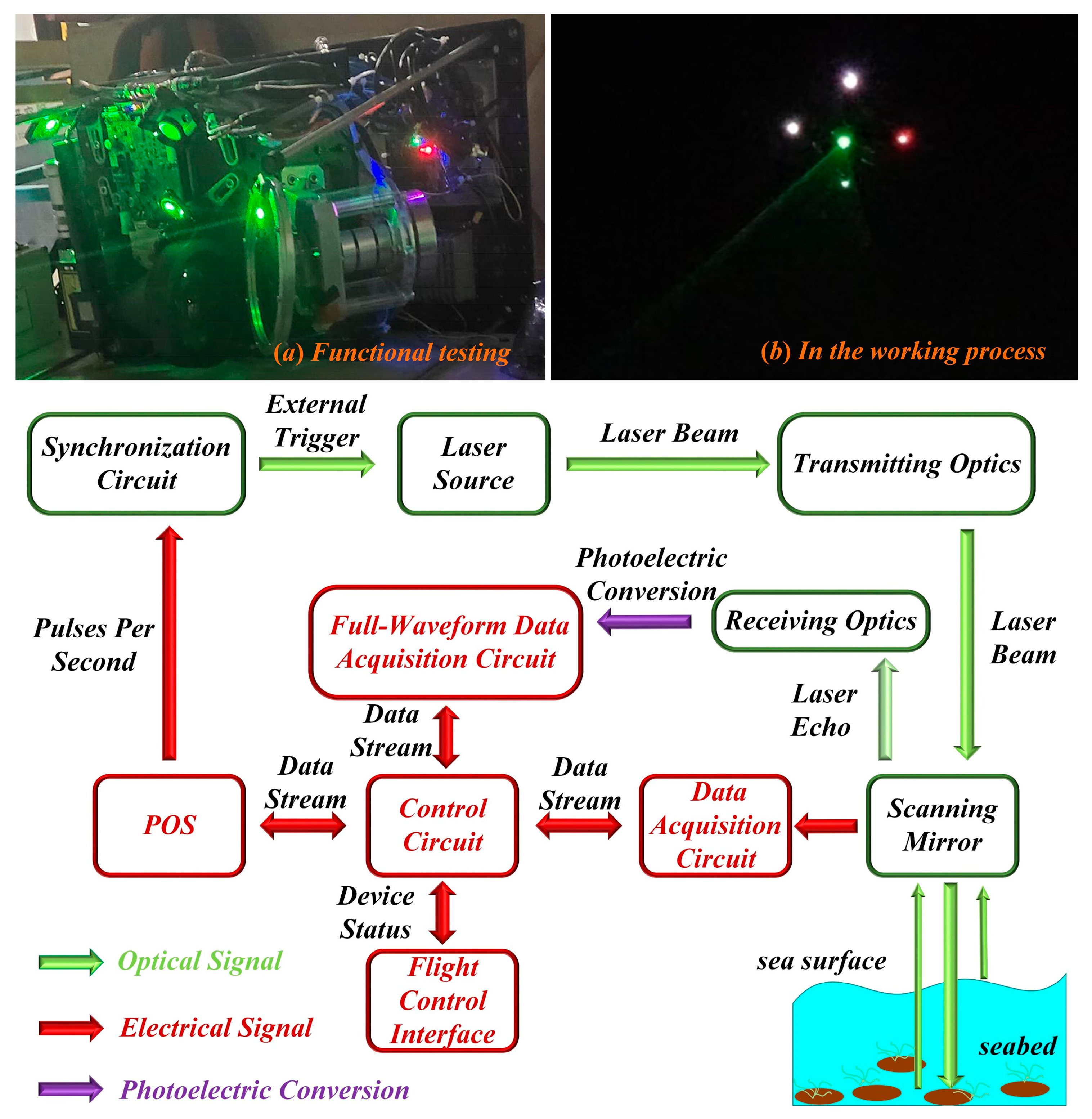
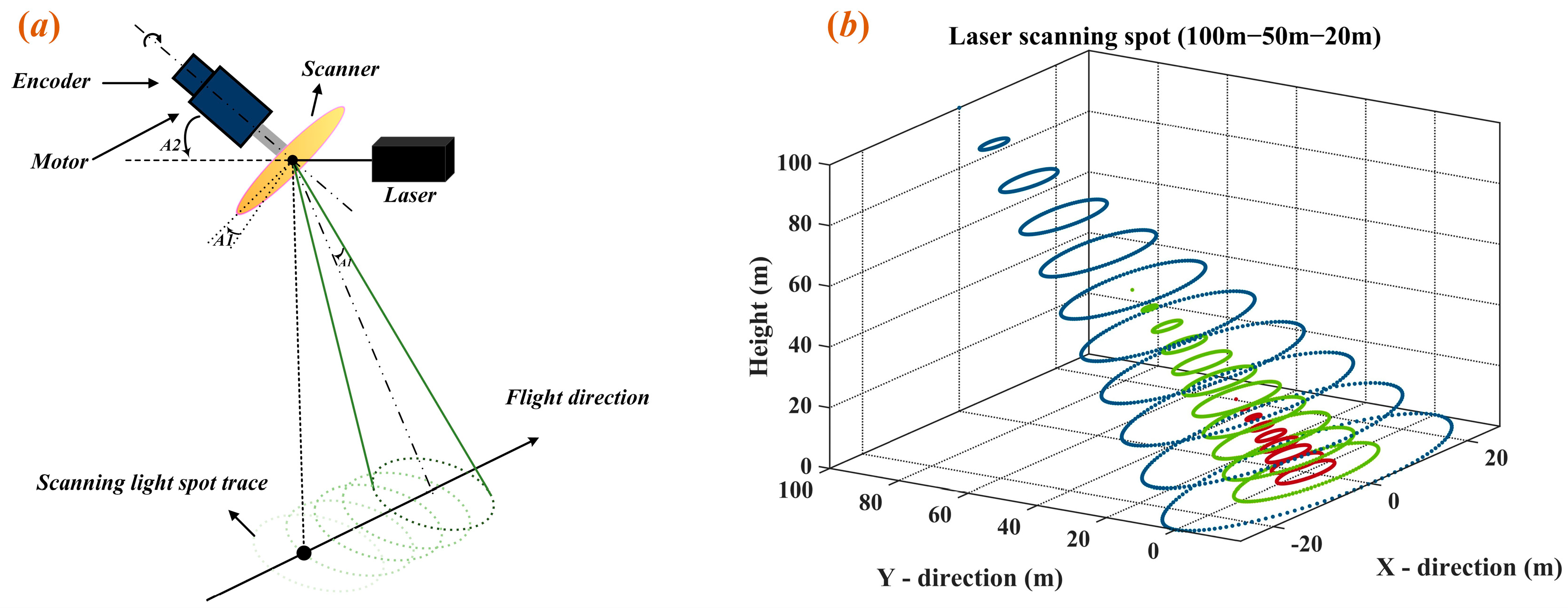
20]. Due to the maturity of research on 532 nm lasers in the blue-green spectrum and their advantages of small size, light weight, and high power, the 532 nm laser is the preferred choice for underwater detection. The airborne laser bathymetry system consists of several key functional units, including optical transmission and reception, data acquisition and control circuits, scanning mirrors, a global positioning system (GPS)–inertial measurement unit (IMU) integrated inertial navigation system, and data processing software. The prototype of the current airborne laser bathymetry system, along with its system composition and operational principles, is shown in
Figure 2. The primary system parameters are listed in
Table 1.
Based on the Beer–Lambert law and incorporating the parameters of typical Jerlov 1 clear coastal water [
21], this study develops a model that captures the multiple scattering characteristics of the experimental system prototype. The model simulates the multiple scattering properties of laser light underwater from a photon perspective. A detailed explanation is provided below.
The computational power of standard computers is insufficient to simultaneously simulate the underwater transmission of hundreds of trillions of photons. The model was simplified to address this limitation and consider the characteristics of laser pulses by grouping all photons into photon packets for a unified motion analysis. The laser emits 5 × 10
3 pulses per second in the current experimental system, with each pulse recording data for 10
3 points. The number of photon packets was set to 5 × 10
6. Tracking the trajectories of millions of photon packets was deemed feasible in terms of both hardware capability and data reliability. An in-depth investigation of multiple scattering processes during the underwater transmission of pulsed lasers is essential for solving the radiative transfer problem [
22]. The unsteady-state solution of the radiative transfer equation can be expressed as follows [
23,
24]:
Here,
is the speed of photon transmission in water,
and
are the beam attenuation coefficient and scattering coefficient, respectively,
is the scattering phase function and describes the probability of scattering from direction
to direction
,
is the irradiance,
is the transmission time, and
and
correspond to the position and direction vectors,
describes the source of radiation at
, position
, and direction
. Based on the radiative transfer equation, seawater parameters, such as scattering and absorption coefficients, water quality, and laser transmission distance, were defined. A Monte Carlo stochastic model was employed to simulate the transmission process of the underwater lasers. The primary initial parameter settings of the model are listed in
Table 2.
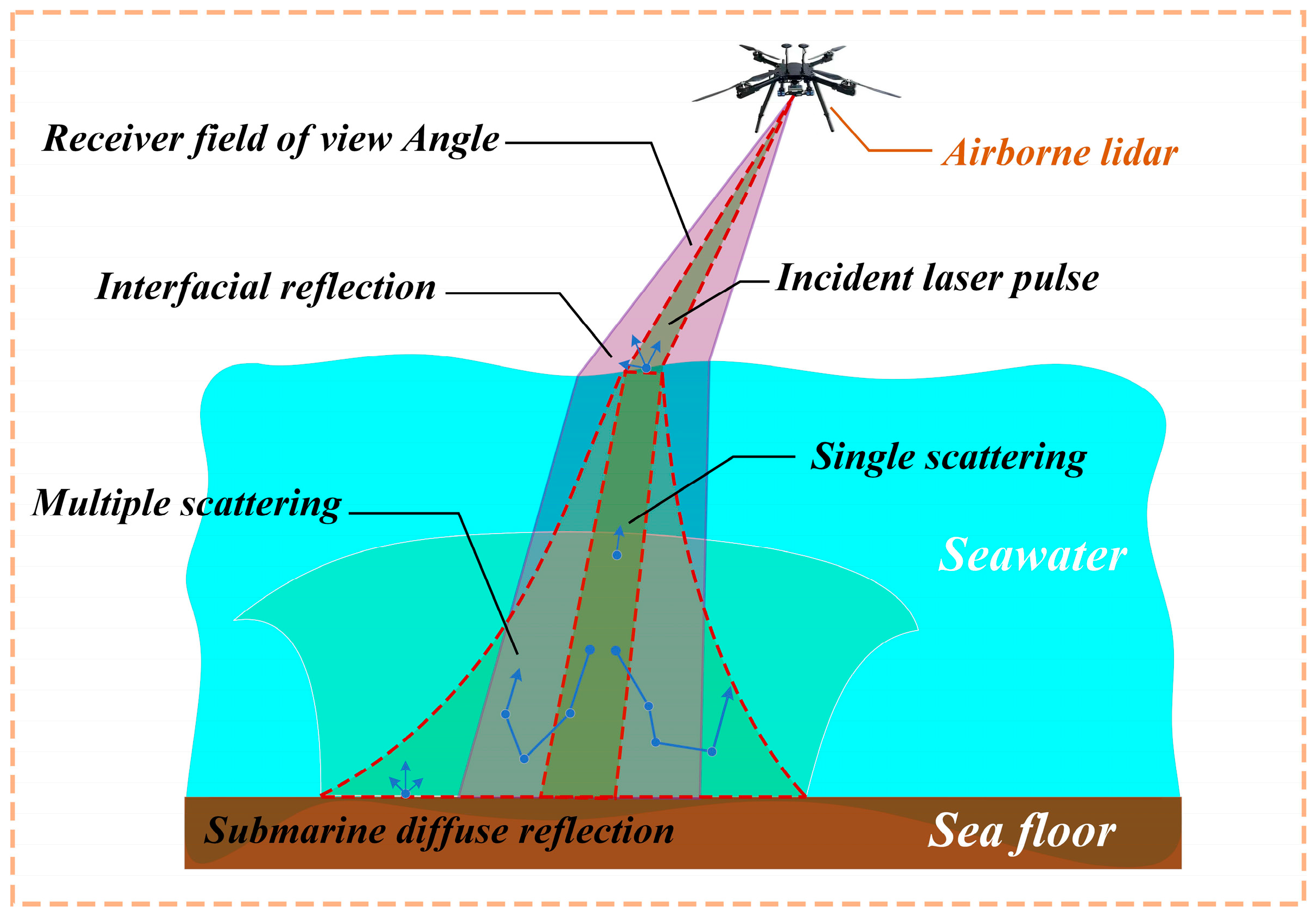
This study proposes a Monte Carlo supervision algorithm that, based on a microscopic analysis model, captures the components of individual photons after scattering, reaching the detector’s receiving plane at different depths. This allows the model to obtain a sufficient number of received signal samples. In the model, the laser beam is assumed to vertically incident downward from the sea surface, with seawater treated as a multilayer structure perpendicular to the beam’s incident direction [
25,
26]. The Monte Carlo stochastic model, constructed based on the optical properties of the seawater medium, enables the precise and efficient simulation of LiDAR transmission signals. However, the model often requires significant computational resources to ensure the reliability of the simulation results [
27,
28,
29,
30,
31].
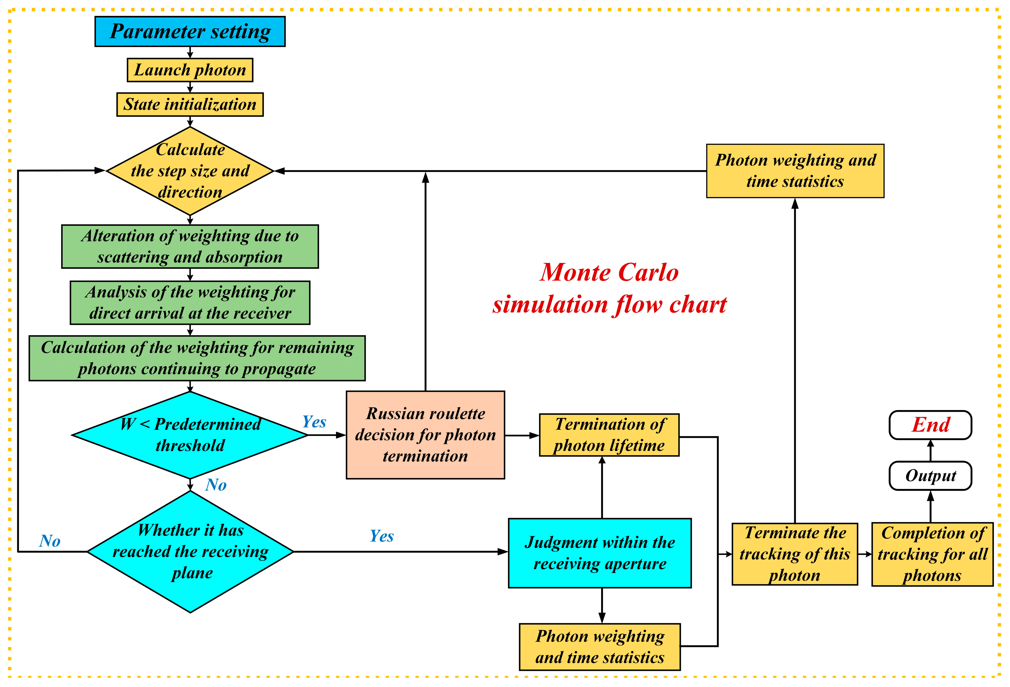
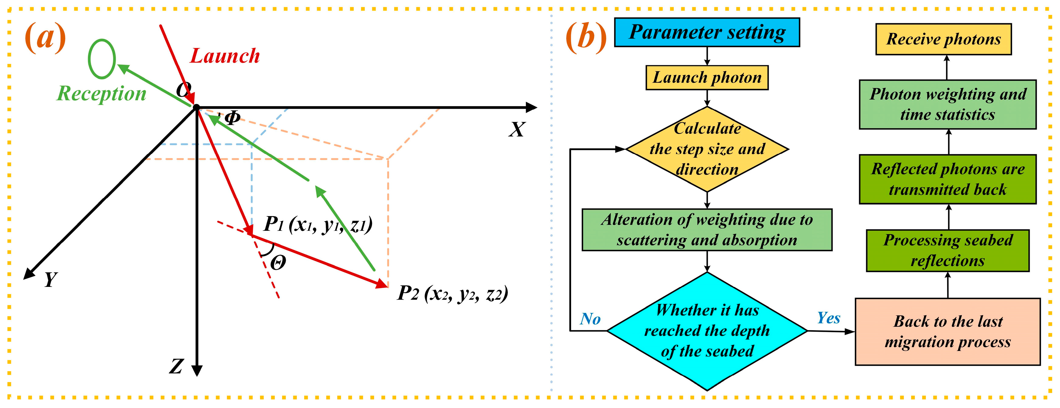
As depicted in
Figure 3, the key steps in implementing the Monte Carlo stochastic model can be succinctly summarized as follows: the photon position coordinates are initialized as
, and the directional cosines of motion are initialized as
. The laser incidence angle is determined by the initial cosine directional components
of the motion vector. The photon energy weight is normalized to
. Let the propagation direction of the photon after scattering be
, and the step length of the photon after the ith scattering be
;
can be determined using Bouguer–Lambert’s law.
In Equation (2), the parameter
represents the total attenuation coefficient of the water body. The current position of the photon is iteratively updated based on its initial position coordinates and directional cosines of motion.
After each collision, the photons are evaluated randomly to determine whether they are absorbed or scattered. A random number
is selected from the interval
and compared with the albedo
. The absorption of a photon is reflected in the change in its energy weight.
In Equation (4),
, where
is the total attenuation coefficient of the water body,
is the absorption coefficient, and
is the scattering coefficient. The photon’s motion is continuously tracked until it is determined whether the photon was annihilated. After a collision, the change in the direction of motion is calculated by sampling the Henyey–Greenstein phase function to determine the azimuth angle
and scattering angle
.
In Equation (6),
is the asymmetry factor of seawater medium and
is a random number uniformly distributed in the interval [0, 1]. The final expressions for the directional cosines of motion can be derived by fixing at the
ith collision point and combining the equations above.
Initially, only single-pass transmission is considered, with photon energy below the lower boundary set to zero, thus halting further migration. The model emphasizes the changes in photon energy resulting from interactions with suspended particles. An improved model is introduced by setting a death threshold,
, to terminate photon tracking when its weight falls below this threshold. It is possible to avoid processing many low-weight photons without losing energy conservation. A Russian roulette mechanism is also incorporated [
32]: if
, photon tracking continues; if
, a random number
is generated and compared with a preset probability threshold
. If
, the photon continues to be tracked with a weight increase of
; otherwise, the photon is considered to have “died” [
33].
For the air/water interface, the change in photon weight and direction of motion can typically be calculated using Fresnel’s reflection law [
34]. However, due to the high frequency of the laser pulse, the time span of each pulse is extremely short, allowing the sea surface to be considered as stationary from a temporal perspective. Additionally, the full waveform data acquired by the LiDAR system clearly reveal distinct peak signals associated with reflections from the sea surface. After time integration, the distance from the radar to the sea surface can be precisely determined. Therefore, our study is confined to the region below the air/water interface, with the initial source position set at
.
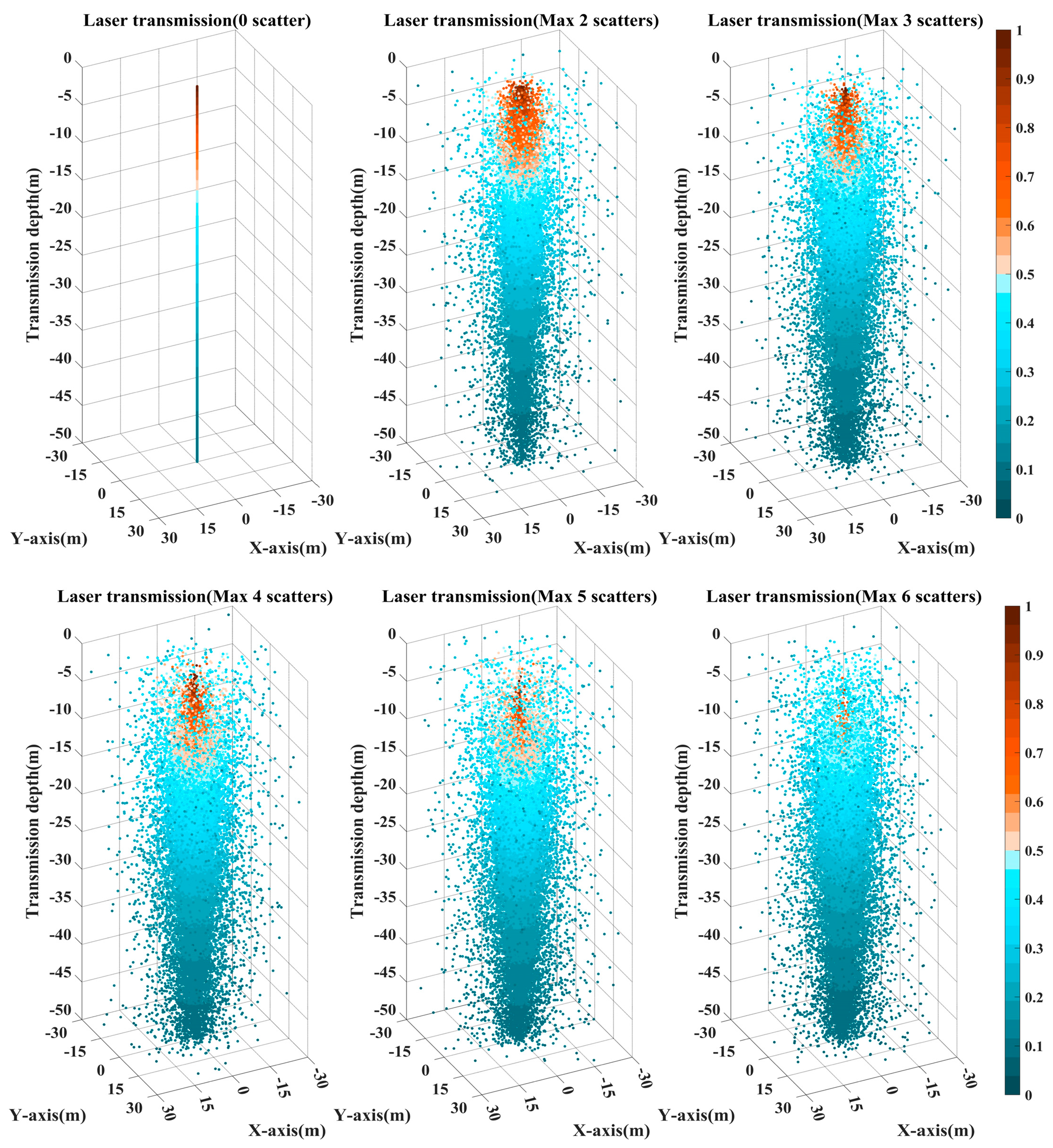
Figure 4 shows the simulation results for the vertical laser incidence and normalized photon energy. As the number of scatterings increases during transmission, the laser beam becomes increasingly divergent, and the photon energy rapidly attenuates with depth. This attenuation follows the Beer–Lambert law [
35]; considering both absorption and scattering, the laser intensity decreases exponentially with increasing transmission distance.
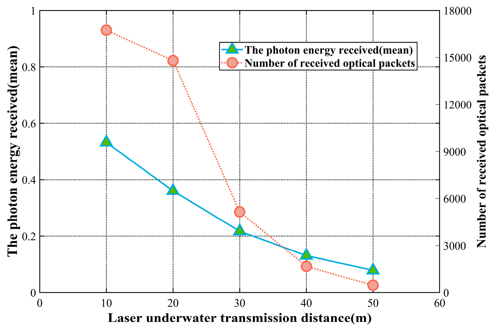
The statistical results for the number of photon packets received and their average energies at different depths are shown in
Figure 5. It can be observed that as photons travel deeper, their energy weight decreases due to scattering and absorption, and the number of photon packets received by the detector decreases even more drastically than the reduction in energy weight. This indicates that a large number of photons are considered “died.” Therefore, tracking only photons with higher weights is more efficient than tracking all photons, and this approach does not introduce significant errors in the results. This also validates the importance of setting the death threshold
.
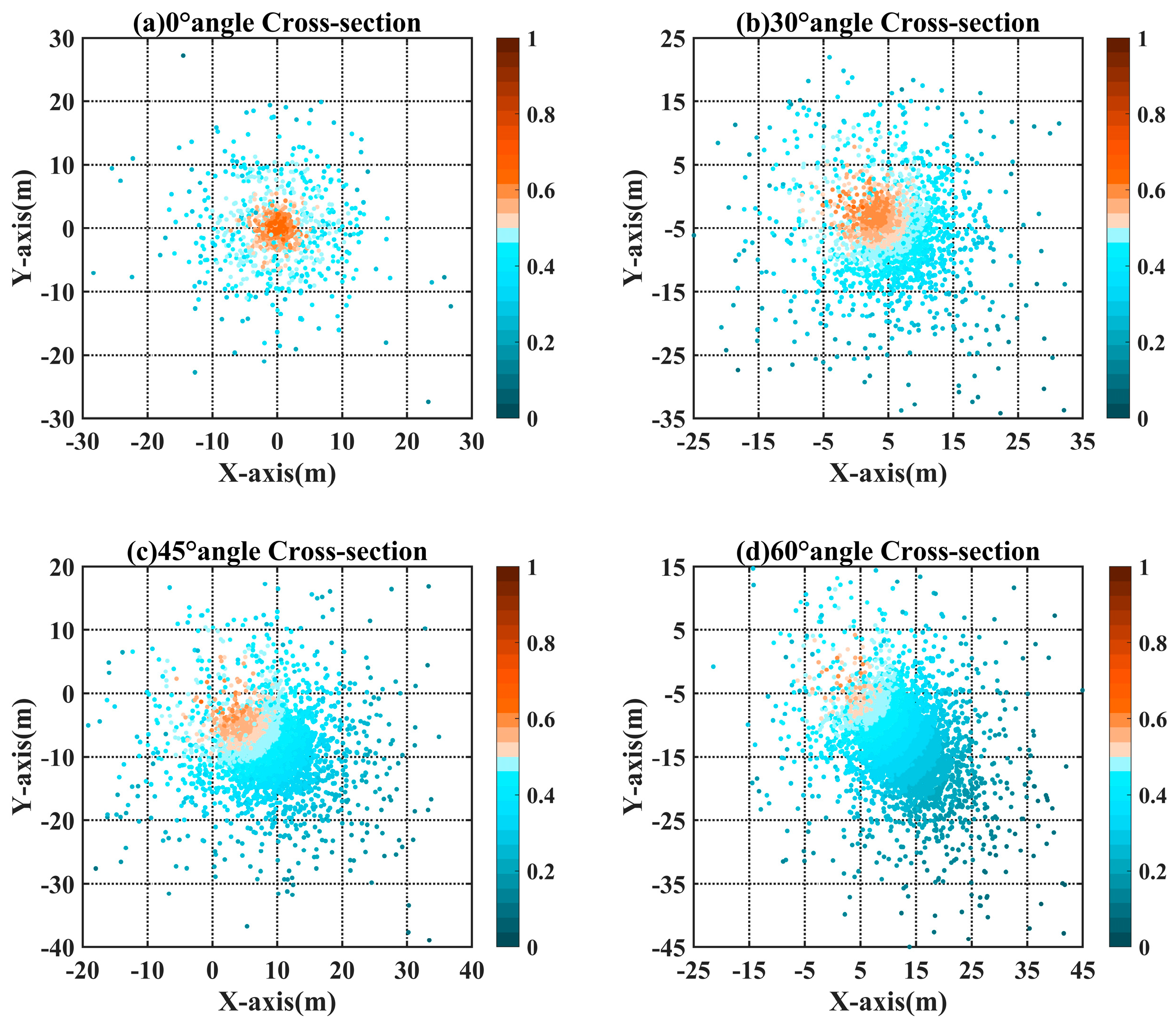
The scanning angle of the experimental system was fixed at 7.5°, resulting in a conical section with a cone angle of 15°. Vertical laser incidence is suitable for the qualitative analysis of underwater targets. However, changing the laser incidence angle for actual measurements is necessary. A comparative analysis was conducted for the typical incidence angles of 30°, 45°, and 60° with respect to the
z-axis to examine the photon spatial distribution and energy variations at a depth of 10 m, as shown in
Figure 6. To maintain consistent visual dimensions across images while accommodating the substantial variation in angle, we standardized the axis lengths and scale. However, we allowed the numerical ranges to vary to preserve detail and avoid obscuring key features.
In
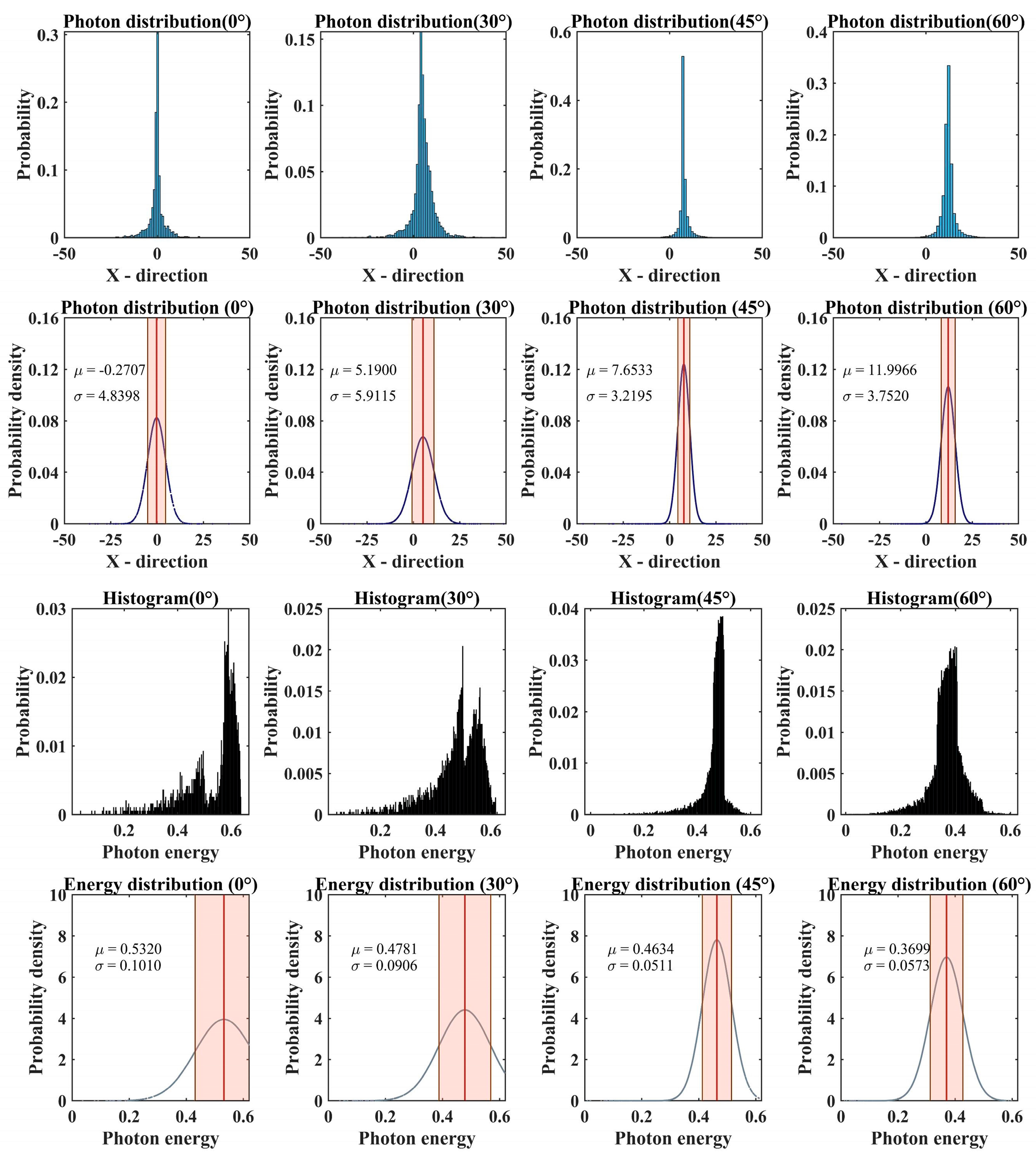
Figure 6a–d, the photon energy shows a significantly banded, uneven distribution. In the case of conventional data processing, only a single scattering process of the laser underwater is considered, not multiple scattering. A quantitative description of this issue is crucial for improving detection accuracy and reducing errors in airborne LiDAR systems. A quantitative analysis of the photon spatial and energy distributions at a depth of 10 m was conducted after the laser entered at different incidence angles. The probability density distribution of the photons in the x-direction within the receiving field of view was processed using a Gaussian function [
32], as shown in
Figure 7.
The results presented in
Figure 7 reveal several intriguing phenomena. The degree of waveform broadening of photons received at a depth of 10 m, following incidence at different angles, did not show a clear trend, indicating the irregular divergence of photons. When the incidence angle ranged from 0° to 30°, the photon distribution diverged. However, the photon distribution shifted toward convergence when the incidence angle increased from 30° to 45°. This phenomenon can be explained as follows: scattering predominates when the incidence angle is between 0° and 30°. In contrast, when it is between 30° and 45°, absorption, influenced by the geometric distance variations caused by the angle, becomes more dominant. Additionally, the irregular fluctuations in the peak can be attributed to the effective absorption of the photons scattered at the edges; this halts their migration and causes the Gaussian waveform to converge toward the center of the symmetry axis. We also observe that the small-angle energy distribution exhibits a bimodal pattern. This can be explained as follows: the smaller the angle, the shorter the path the beam travels to reach a given depth. The high-energy peak indicates that the photons undergo fewer scattering events between emission and reception. As the incident angle increases, the path length increases, and the high-energy peak gradually shifts towards the low-energy peak, eventually merging into a single peak.
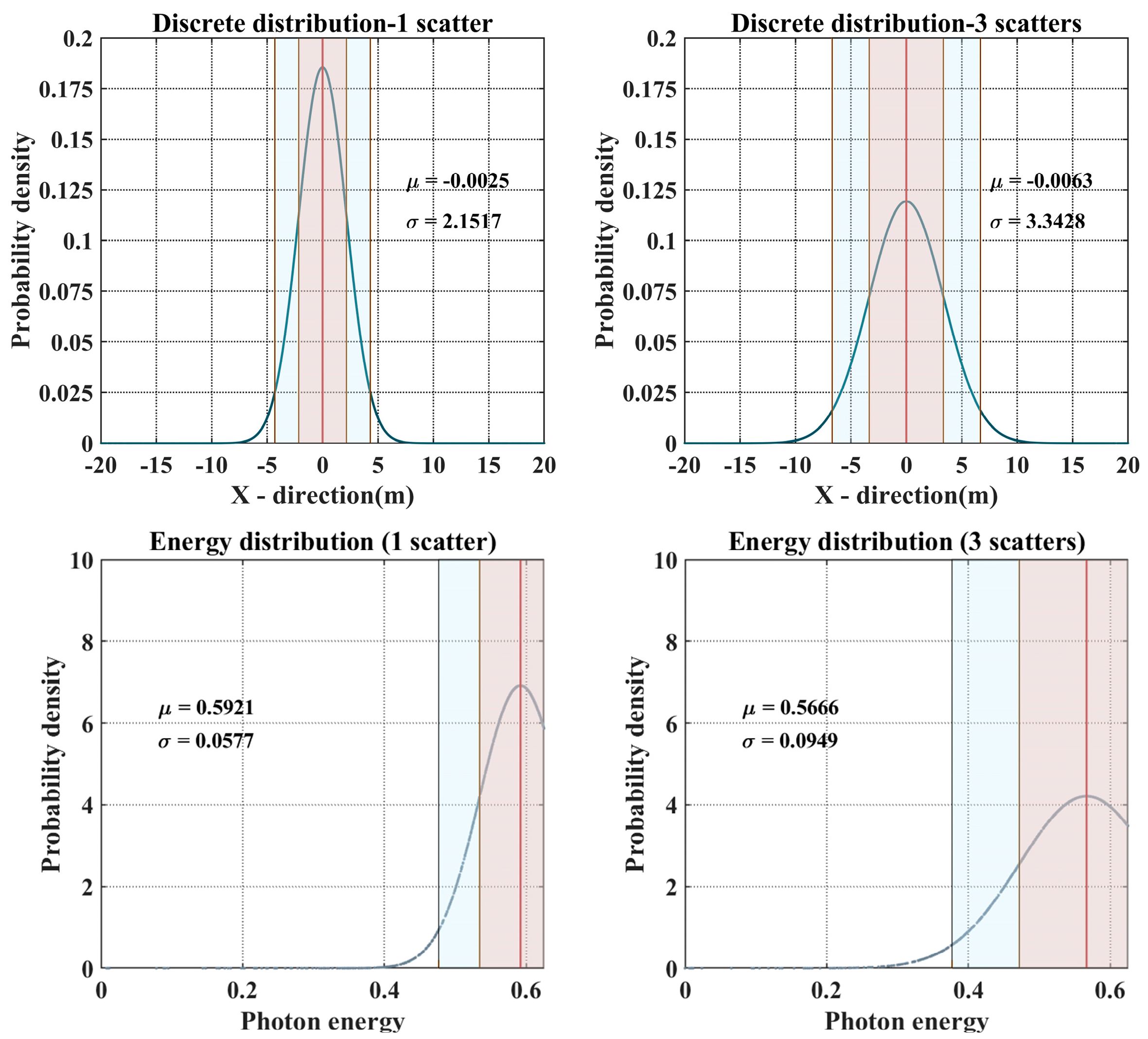
The classical lidar equation considers only a single backscattering event. In practice, however, particularly for underwater laser transmission, photons undergo multiple small-angle scatterings, deviating from straight-line propagation. This weakens the main beam, reduces the effective return signal, and degrades range resolution. Spatially, increased stray light and a lower proportion of target-return photons lead to image blurring and greater ranging errors. Given these conditions, a statistical analysis of photon scattering and energy variation is required. These effects can be mitigated by Monte Carlo simulations, which trace individual photon paths and their associated energy losses to enable more accurate modeling of scattering dynamics.
Figure 8 depicts the Gaussian distribution of the photon simulations for single scattering and three scattering events. Given a sufficiently large reception field of view, specifically one that encompasses the sea surface scanning range of the airborne sonar radar at an altitude of 50 m, the coverage area approximates an ellipse with a semi-major axis of 15 m; the error primarily stems from energy loss. By considering both the distribution of received photons and their energy characteristics at a depth of 10 m, the correction factor for errors caused by scattering can be derived as follows:
In Equation (8),
represents the total error correction factor, while
refers to the scattering distribution error caused by different numbers of scattering events. This can be calculated as the ratio of the variance of the position distributions for three scattering and single scattering events,
.
represents the energy loss of photons, which directly affects the estimation of detection depth. This can be derived from the change in the mathematical expectation of the energy Gaussian distribution,
. Therefore, based on the results in
Figure 8, it can be concluded that considering three scattering events, compared to considering only single scattering, can correct at least 6.992% of the error for detecting targets at a depth of 10 m. Considering the Monte Carlo error quantification, increasing the simulation runs and introducing a 95% confidence level, the error range is 6.992% ± 0.3%.
2.2. Simulation and Analysis of Temporal Broadening Characteristics of Laser Transmission Underwater
Interactions with suspended particles in seawater occur during the underwater transmission of a laser pulse. These interactions lead to two main effects: first, they cause the laser beam to diffuse during transmission, and second, multiple scattering results in multipath transmission, which causes temporal broadening of the laser pulse signal [
35]. Since the H-G phase function is the preferred choice for simulating seawater scattering characteristics using the Monte Carlo method, this study combines it with Monte Carlo simulations to analyze the temporal broadening of laser pulse underwater transmission. An innovative approach is proposed by describing the temporal broadening of the waveform using the probability corresponding to the transmission time to the receiving plane. Compared to using amplitude as the vertical axis, this normalization method more effectively reflects the interactions occurring during laser underwater transmission. The factors influencing pulse broadening are then analyzed, starting with the impact of laser underwater transmission distance on pulse broadening.
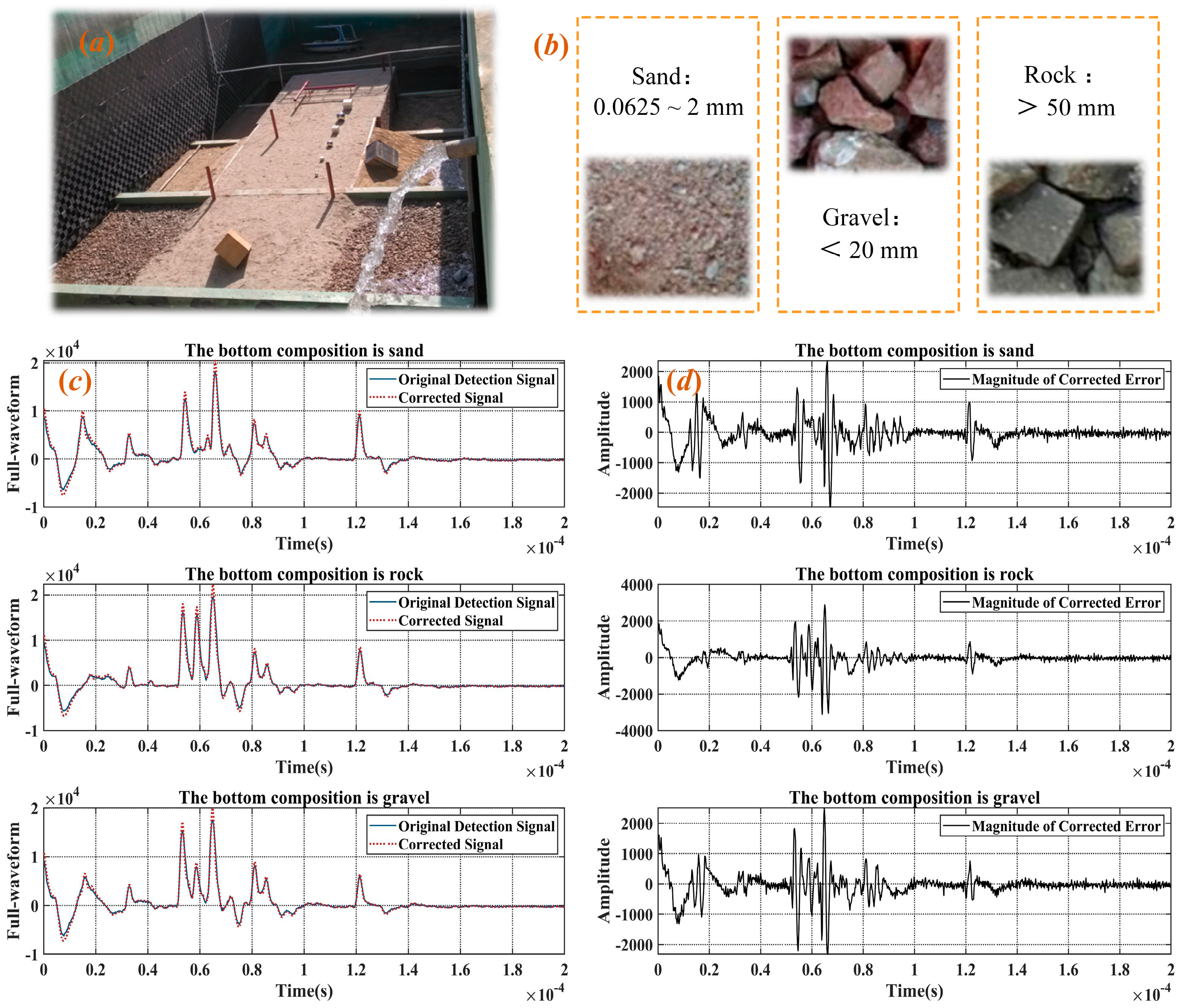
At 40 cm and 50 cm underwater, detection planes were established while keeping the environmental parameters and other model conditions unchanged. The Monte Carlo random model simulation results for the pulse-broadening waveforms are shown in
Figure 9a,b. A comparison of the two figures reveals that as the underwater laser transmission distance increased, the number of scattering events also increased, leading to a longer time from the start to the end of the pulse recording. The simulated waveform results closely match the actual detection scenarios, as shown in
Figure 9c. Although the actual underwater transmission distances during testing were relatively short, a detailed analysis of the changes in a specific half-wave peak revealed that the magnitudes of broadening were comparable. It should be noted that individual pulses exhibit significant randomness. To improve reliability,
Figure 9a,b show the temporal broadening based on the accumulation of 10 pulses.
Figure 9c presents the pulse broadening observed during actual detection. Notably, to better resolve the characteristics of different seabed substrates, the experiment was conducted in relatively shallow water, resulting in a shorter laser propagation time. However, given the system’s pulse repetition rate of 5 × 10
3 pulses per second, the integrated pulse signals yield time scales comparable to those observed in the simulation. In addition, the calculations indicate that the maximum effective temporal broadening is approximately five nanoseconds, corresponding to the longest optical path length. The simulation results and experimental results are of the same order of magnitude [
16]. This consistency underscores the ability of the model to accurately simulate the temporal broadening characteristics observed in the practical experiments.
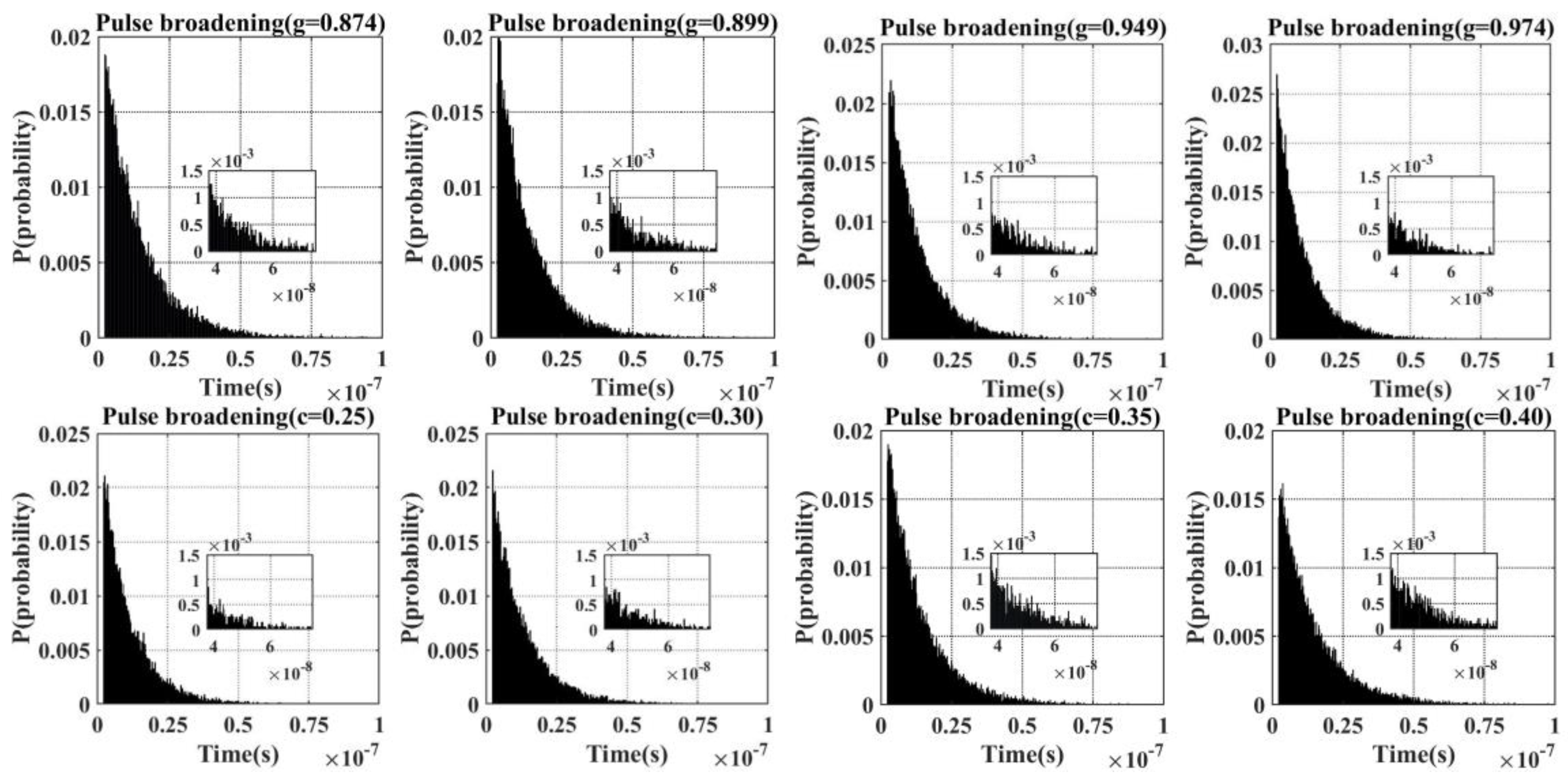
The asymmetry factor,
, characterizes the forward-scattering properties of seawater. The H-G phase function flexibly characterizes the angular distribution of scattering using the asymmetry parameter
. When
, forward scattering predominates, making it suitable for modeling typical particles in water. For airborne LiDAR bathymetry systems primarily utilized in shallow coastal waters with significant spatial variability in water quality, studying the influence of g on temporal pulse broadening is crucial for improving the detection performance of current experimental prototypes as shown in
Figure 10, using g = 0.924, which most closely matches Petzold’s measured water quality parameters [
36]. With deviations of ±0.025 and ±0.05, it is observed that larger asymmetry factors lead to reduced pulse broadening. The calculations indicate that increasing the asymmetry parameter g from 0.874 to 0.974 results in a 2.5-nanosecond decrease in temporal pulse broadening. This occurs because stronger forward scattering in seawater shortens the path length of scattered photons before they reach the detector’s photosensitive surface, thereby minimizing temporal spread [
36]. In the Monte Carlo random model, the seawater attenuation coefficient c governs the photon free path length, S. By maintaining consistent underwater environmental parameters and system conditions, simulations performed with c values of 0.25, 0.3, 0.35, and 0.4 demonstrated that an increase in the effective attenuation coefficient led to a more pronounced temporal broadening of the laser pulse. The calculations indicate that increasing the asymmetry parameter c from 0.25 to 0.4 results in a 3.5-nanosecond increase in temporal pulse broadening. This is because a larger attenuation coefficient shortens the average photon migration step length, increases the number of scattering events over the same transmission distance, and thereby results in more pronounced temporal broadening of the pulse. The model also demonstrates strong scalability, offering potential for future optimization of critical ALB system parameters, including scanning angle and pulse frequency, to improve detection performance and data fidelity.
2.3. Simulation and Analysis of Airborne LiDAR Echo Light Reception Probability
To obtain underwater topographic information, an active airborne LiDAR bathymetry system requires receiving echo light and converting it into electrical signals after laser emission. However, most previous studies primarily focused on simulating the laser emission process using Monte Carlo methods, with little attention paid to modeling the echo light reception path in certain scenarios [
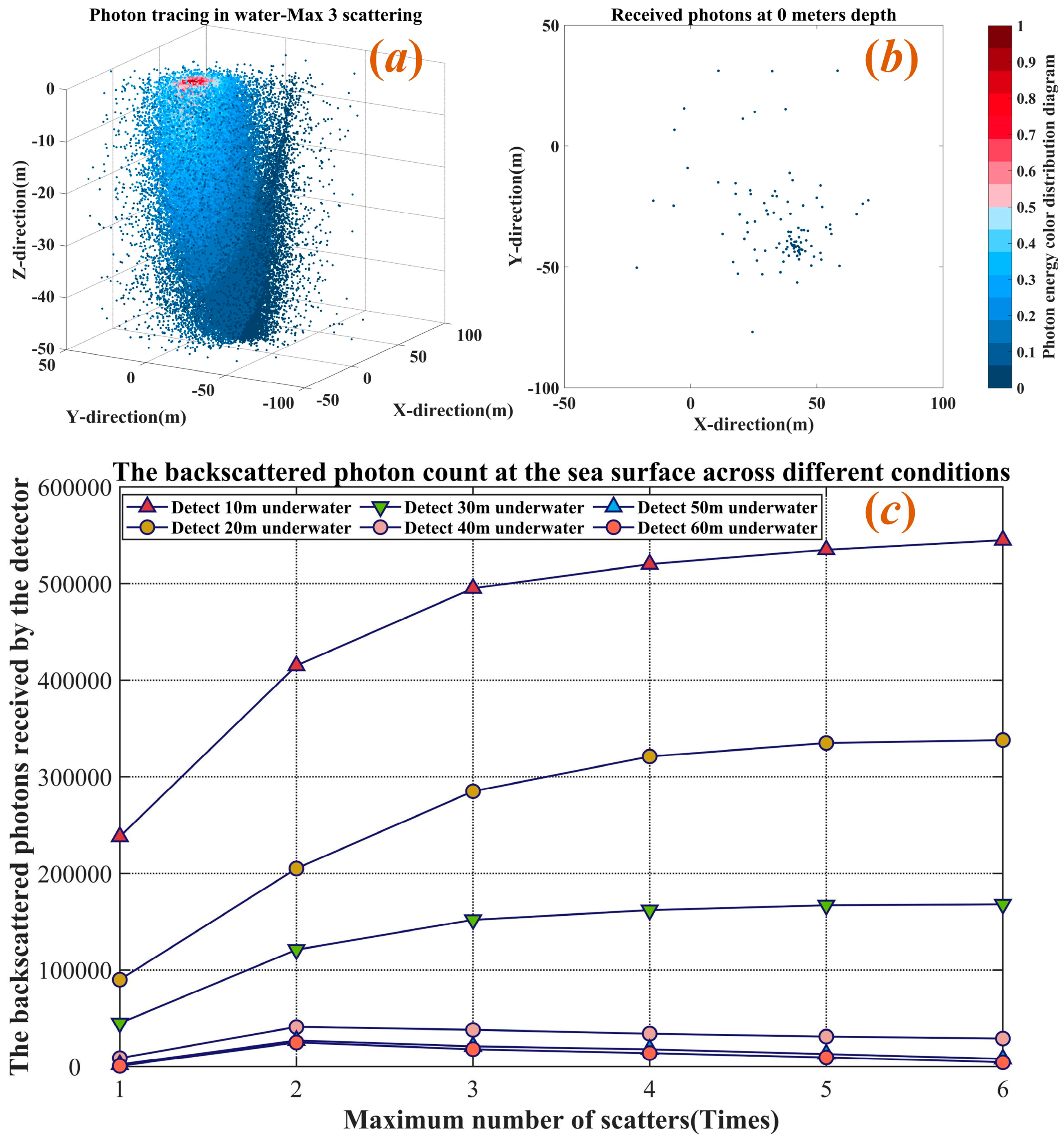
37]. Therefore, simulating echo light reception probability using a Monte Carlo stochastic model is a novel research direction. By positioning the detection plane on the same level as the laser emission source, this study analyzed the probability of laser echoes returning to the receiving plane in an airborne LiDAR system.
The process of echo light reception, indicated by the green arrows in
Figure 11a, involves the deflection of the laser light after interacting with a target at a certain depth. Based on the Monte Carlo random model, selecting the “seafloor” location, and placing a detector at the laser emission point to record photons that return to the sea surface. This introduces two main issues. First, the model predicts laser transmission from the perspective of photons, with the photon trajectory determined by randomly sampled directional cosines and migration step lengths. Determining whether a photon has reached the seafloor interface is challenging. The second issue is the design of the detection plane and filtering out non-seafloor echo lights. Solving these two problems is crucial for practically detecting the entire experimental system.
In response to these issues, the methods and modeling workflow illustrated in
Figure 11b were implemented. The model assumes the seafloor is 50 m below the water surface [
38], with the seafloor being a Lambertian surface [
39]. Upon reaching this depth, the incident light beam undergoes reflection. The inverse processing is applied to the Si step at which the light reaches the seafloor. The model identifies the photon’s z-coordinate after the
ith migration using seafloor depth as a threshold. If it exceeds the seafloor depth, the model traces back to the coordinates after the (
i − 1)th migration. If the value is below seafloor depth, the photon is considered to have crossed the seafloor during that step. The initial coordinates of this step are then retrieved using boundary processing at seafloor depth. The scattering and azimuth angles are also sampled, and the total laser emission time is recorded. The simulation results of the detector receiving the echo light are shown in
Figure 12. Few photons returned to the sea surface and were detected by the receiver. It must be noted that the detector area provided in this study is sufficiently large.
Although the actual number of photons may vary due to absorption or scattering, the normalized results presented in
Figure 8 may obscure these changes, as all values are scaled to a uniform range. Therefore, it is essential to statistically track the number of photons received by the detector. The data in
Figure 12 show that as the number of scatterings increased, the number of photons received by the detector at the sea surface followed a similar trend for the underwater transmission distances of 40, 50, and 60 m. However, at a 10, 20, and 30 m transmission distance, the number of received photons and the overall trend changed significantly, which is intriguing. This can be attributed to the 30 m depth limit, which restricts the photons from completing their full trajectory. In other words, under the current mathematical model, the “scattering potential” of the photons is not thoroughly exhausted. When photons return to the receiving plane, their migration step lengths are determined. This indirectly confirms that the Monte Carlo random model is well suited for coastal waters shallower than 30 m. This aligns well with the operating domain of marine LiDAR, in which photons remain in a state always subject to scattering. This is closer to the actual measurement situations, and fully exhausting the photon’s “scattering potential” may introduce substantial errors.


