Article

Multi-Level Intertemporal Attention-Guided Network for Change Detection in Remote Sensing Images

1
The Department of Electronic Engineering, Chengdu University of Information Technology, Chengdu 610103, China
2
Shaanxi Key Laboratory of Network Data Analysis and Intelligent Processing, School of Computer Science and Technology, Xi’an University of Posts and Telecommunications, Xi’an 710121, China
3
The First Geolnformation Mapping Institute of Ministry of Natural Resources, Xi’an 710054, China
*
Author to whom correspondence should be addressed.
Remote Sens. 2025, 17(13), 2233; https://doi.org/10.3390/rs17132233
Submission received: 28 April 2025 / Revised: 26 June 2025 / Accepted: 26 June 2025 / Published: 29 June 2025

Abstract

Change detection (CD) is detecting and evaluating surface changes by comparing Remote Sensing Images (RSIs) at different times, which is of great significance for environmental protection and urban planning. Due to the need for higher standards in complex scenes, attention-based CD methods have become predominant. These methods focus on regions of interest, improving detection accuracy and efficiency. However, external factors can introduce many pseudo-changes, presenting significant challenges for CD. To address this issue, we proposed a Multi-level Intertemporal Attention-guided Network (MIANet) for CD. Firstly, an Intertemporal Fusion Attention Unit (IFAU) is proposed to facilitate early feature interaction, which helps eliminate irrelevant changes. Secondly, the Change Location and Recognition Module (CLRM) is designed to explore change areas more deeply, effectively improving the representation of change features. Furthermore, we also employ a challenging landslide mapping dataset for the CD task. Through comprehensive testing on two datasets, the MIANet algorithm proves to be effective and robust, achieving detection results that are either better or at least comparable with current methods in terms of accuracy and reliability.

1. Introduction

Change detection (CD) in Remote Sensing Images (RSIs) refers to the process of extracting changed regions from two or more RSIs of the same scene at different time phases. Among them, multispectral RSIs contain crucial information about the color, texture, and material properties of imaging objects, without significantly increasing the data dimension. Therefore, CD in RSIs is widely applied in urban planning [1,2,3], disaster assessment [4,5,6], resource investigation [7,8,9], etc.
Currently, methods for CD in RSIs have been extensively studied [10,11]. Early classical CD methods include algebra-based methods [12] and transform-based methods. However, these traditional CD methods often rely on manual feature acquisition, leading to limited detection accuracy. Deep learning-based CD methods have become the mainstream approach in increasingly complex CD scenarios, surpassing traditional methods with their powerful feature extraction capabilities and efficient detection performance [13]. The powerful representation ability of CNNs significantly enhances the detection performance of the model. Daudt et al. [14] proposed a fully convolutional network to address the CD problem. They employed a training approach exclusively based on the CD dataset, resulting in superior detection performance compared to traditional methods relying on transfer learning. Rahman et al. [15] proposed a Siamese network that was trained using simulated images, overcoming the lack of a large annotated satellite dataset.
Subsequently, attention mechanisms have garnered attention in CD due to their ability to automatically focus on relevant information while filtering out irrelevant data. Researchers have started integrating attention mechanisms into CD models to enhance the effectiveness of feature extraction. Liu et al. [16] introduced a stacked attention module to solve the problem of different resolutions in high-resolution image CD tasks. Zhang et al. [17] combined CNN and transformer, which not only focused on local features but also realized long-distance information interaction, which greatly improved the algorithm’s efficiency. Lv et al. [18] proposed a network for CD that achieved multi-scale information fusion through UNet and a multi-scale information attention module. They also constructed a location channel attention to focus on the location information of change features.
However, RSIs are typically acquired at different time phases. In practical applications, numerous unexpected changes will be introduced by seasonal changes, changes in lighting conditions, and architectural renovation, which will interfere with the detection results. Current algorithms primarily focus on extracting features from either the channel or spatial dimensions of the bi-temporal images, neglecting the richer spatio-temporal variation information available. Moreover, the interference of irrelevant changes also requires early feature interactions to propagate their respective spatial information, enabling the model to concentrate on the pertinent areas of change. In addition, after feature encoding, accurately detecting multi-scale change regions requires the model to have higher precision in region detection.
Therefore, this paper proposes a MIANet for CD. MIANet is based on the lightweight A2Net network [19] and employs the MobileNetV2 lightweight encoder to encode features. This is followed by a Layer Neighborhood Aggregation (LNA) operation, which effectively fuses adjacent layers’ features. This approach allows for a deeper exploration of the complementary information between low-level features and high-level semantic features, capturing richer spatio-temporal variations. To mitigate interference from irrelevant changes, MIANet incorporates an IFAU. This unit enhances early feature interactions, facilitating a more accurate focus on regions of interest and improving the overall expression capability of change features. Furthermore, the network includes a CLRM that incrementally searches for change features across feature maps of different scales using dilated convolution. The Coordinate Attention Mechanism (CAM) [20] within this module ensures precise location and recognition of changed areas, thereby enhancing the accuracy of multi-scale CD. Finally, a Supervised Attention Module (SAM) [19] is introduced to reweight features to achieve multi-level feature aggregation from the high level to the low level. Experimental results on LEVIR-CD and GVLM datasets show that the proposed method improves the CD performance.
In summary, the significant contributions of the MIANet method can be described as follows:
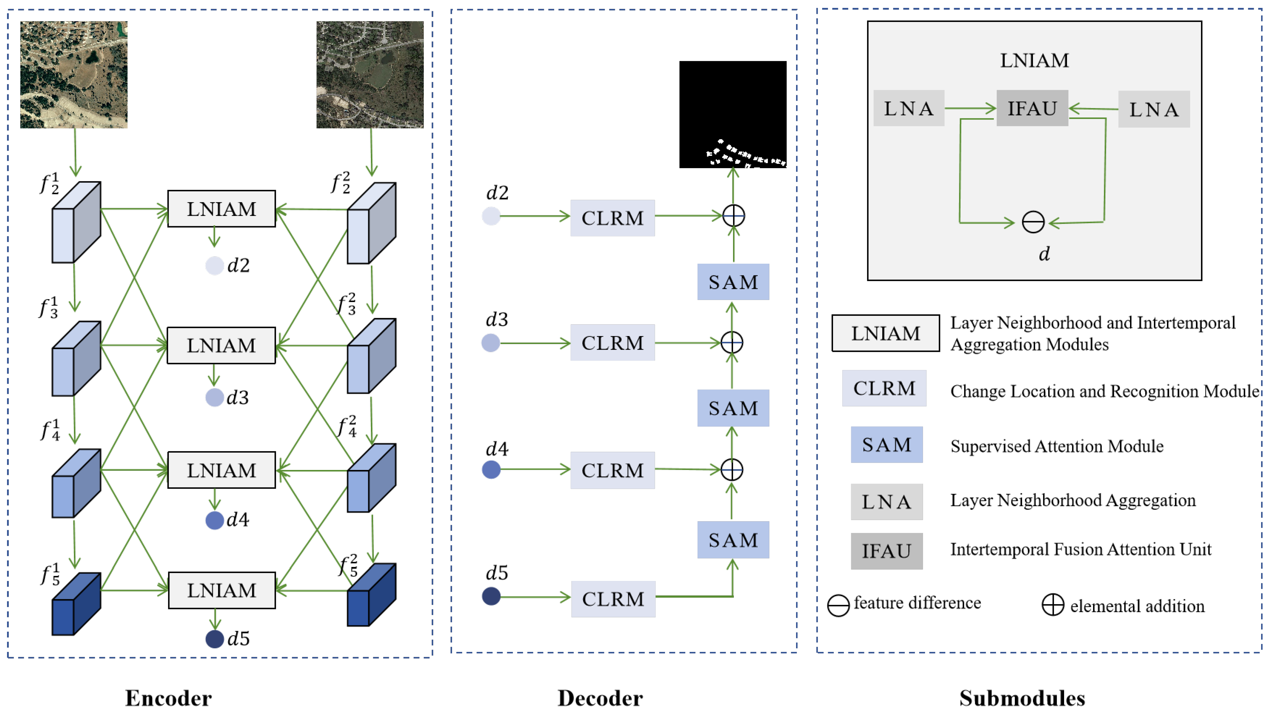
  • We propose an IFAU that leverages the change information in feature maps at different time phases to guide the attention matrix. This approach effectively mines early correlation information between bi-temporal images and efficiently suppresses the influence of irrelevant changes.
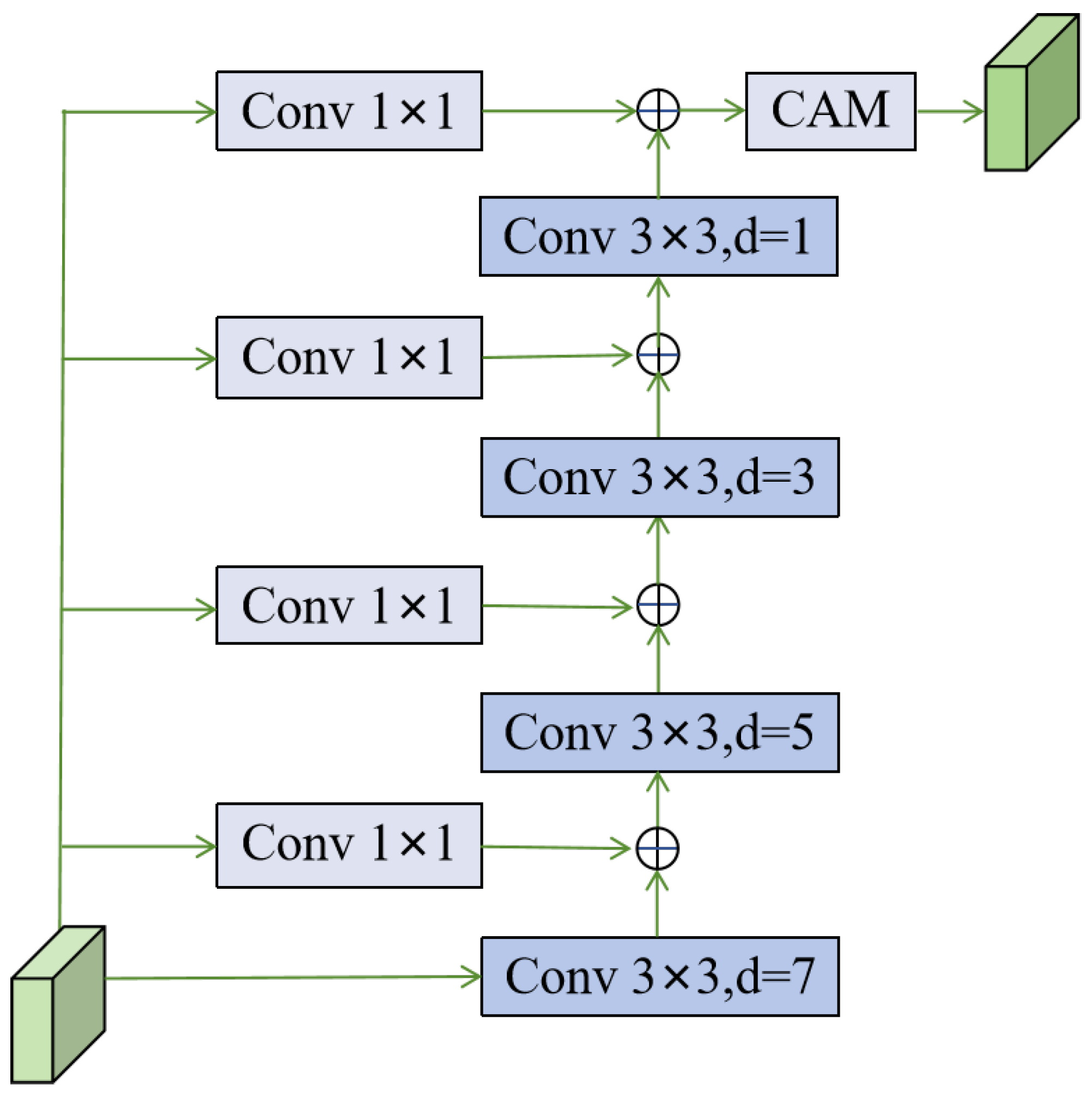
  • We present a CLRM that investigates change information using dilated convolutions on multi-scale feature maps, while CAM is employed for precise localization and recognition of the change areas.
  • The proposed algorithm demonstrates robust performance in complex scenes, as evidenced by the experimental results obtained on the challenging GVLM dataset.

2. Related Work

2.1. Attention Mechanism

Attention mechanisms aim to emulate human attention behaviors in reading and listening, enabling efficient allocation of information processing resources. They originated from research on human visual cognition and were initially proposed in the context of visual imagery [21]. The combination of attention mechanisms and deep networks has effectively improved the performance of computer vision. Hence, attention mechanisms have been widely employed in image classification and semantic segmentation [22,23,24]. The common attention mechanisms include spatial attention, channel attention, temporal attention, channel–spatial attention, and spatial–temporal attention.
The purpose of the channel attention mechanism is to explore the importance of each channel. The representative model is Squeeze-and-Excitation Networks (SENets) [25]. A SENet consists of two main components: compression and excitation. The compression phase aims to condense global spatial information, followed by feature learning in the channel dimension. During the excitation phase, weights are allocated to each channel based on its significance, which results in the generation of the channel attention map.
The spatial attention mechanism focuses on the internal correlation between the location of the information and the feature space, which is closely related to the objective of CD: determining where the change occurs. Similar to the channel attention mechanism, the spatial attention mechanism utilizes max pooling and average pooling in the channel dimension to learn spatial features. A representative model incorporating this mechanism is the Spatial Transformer Network (STN) [26]. The purpose of the STN is to address the issue of reduced classification accuracy in the model caused by transformations such as translation, rotation, scaling, and other operations applied to the input image.
The classic model of channel–spatial attention mechanism is the Convolutional Block Attention Module (CBAM) [27], which is a combination of the channel attention mechanism and spatial attention mechanism. The image is first processed through the channel attention module, which enhances feature representation across different channels. Subsequently, the spatial attention mechanism extracts key information from different locations.

2.2. Deep Learning-Based Change Detection Methods

Recently, deep learning has attracted extensive attention from scholars in the field of CD because of its automatic feature extraction and powerful representation ability. At present, the methods of CD can be roughly divided into CNN-based methods, attention-based methods, and transformer-based methods.
In the early years, CNNs were easy to implement due to their simple structure. Daudt et al. [28] proposed a fully convolutional CD network trained end-to-end. Building on this, encoder and decoder structures were combined to extract and recover multi-scale features through skip connections [14], further enhancing the performance of CD. While CNNs perform well in detecting large changes, they may fall short in capturing small changes.
Because the attention mechanism focuses on the useful information in the image and disregards the irrelevant information, it enables the model to better capture subtle change features. Song et al. [29] utilized spatial attention and channel attention modules to enhance the differential expression between changed objects and the background, which played a crucial role in the CD for RSIs. Zhou et al. [30] adopted a multi-head attention mechanism to fully exploit temporal information, reduce imaging differences, mitigate imaging interference and class imbalance problems, and obtain more comprehensive multi-scale information. To address the inefficiency of aggregating local features and contextual information, Li et al. [31] proposed a pyramid pooling dynamic sparse attention mechanism to capture multi-scale context information and accurately detect the local details of changing regions. To reduce learning bias and tackle the issue of small training datasets, Noman et al. [32] implemented sparse attention operations to focus on selected information regions, capturing inherent characteristics prevalent in CD datasets, effectively suppressing noise interference, and enhancing relevant semantic changes.
The vision transformer uses a self-attention mechanism to capture dependencies between different locations and can be calculated in parallel. Compared to convolutional neural networks, the transformer model is increasingly used in remote sensing CD. Chen et al. [33] proposed a bi-temporal RSI transformer that models the spatio-temporal context through a transformer encoder and uses a transformer decoder to refine the original features, achieving differential expression of objects with the same semantic concept. Bandara et al. [34] proposed a transformer-based Siamese network for CD, which integrates a hierarchical transformer encoder with a multi-layer perceptron decoder to efficiently calculate multi-scale feature differences. Zhang et al. [35] designed a Siamese U-shaped structure, using Swin transformer blocks as basic units to effectively capture global information. Yan et al. [36] employed the Swin transformer for multi-level feature extraction, followed by feature enhancement and change prediction. Li Z et al. [37] proposed the STADE-CDNet model to extract key features from the disparity map using the CD disparity enhancement module. Y. Chen et al. [38] proposed a CD model based on Fourier feature interaction with multi-scale sensing, which utilizes the Fourier transform to adaptively mine the temporal phase information of features in the frequency domain. Chen H et al. [39] introduced the Mamba architecture based on state-space modeling to the remote sensing CD task for the first time. Visual Mamba was adopted as an encoder to realize efficient interaction of multi-temporal phase features. They further introduced an attention module and combined multiple loss functions to improve detection results. However, most current attention mechanism-based methods fail to construct a comprehensive model that integrates spatial, spectral, and temporal information. The integration of attention mechanisms in CD tasks can often present significant challenges related to memory and computational costs. Therefore, it is crucial to investigate further the combination of attention mechanisms with CD tasks.

3. Method

This section provides an overview of the network structure of the proposed MIANet. Following this, the structure and function of each module within the network are described in detail.

3.1. Network Architecture

As shown in Figure 1, the proposed method uses an encoder–decoder structure. The encoder utilizes MobileNetV2 [40] to extract multi-level features from the bi-temporal image. Subsequently, it integrates Layer Neighborhood and Intertemporal Aggregation Modules (LNIAMs) to enhance feature expression capabilities. The decoder includes two basic units: CLRM and SAM collaborate to fuse multi-level features, enabling the prediction of a change map with rich details.

3.1.1. Encoder

The primary function of the encoder is feature extraction. While utilizing VGG and ResNet structures in the encoder–decoder network enhances CD performance, it also consumes substantial computational resources, thereby compromising detection efficiency. Consequently, in this study, the lightweight network MobileNetV2 was chosen for feature extraction within the encoder. The global average pooling layer and the last fully connected layer of the MobileNetV2 encoder were removed to accommodate the CD task. Firstly, the bi-temporal images were input into the encoder, and in the resulting five-layer feature pairs ( f 1 1 , f 1 2 ) , ( f 2 1 , f 2 2 ) , , ( f 5 1 , f 5 2 ) , the size of each layer’s features was halved compared to the preceding layer. To improve efficiency, the features of the last four layers were applied to CD.
The LNIAM is proposed to address the diminished feature representation capability resulting from the lightweight nature of the MobileNetV2 encoder. To compensate for this limitation, these modules integrate adjacent layer features and bi-temporal features, thereby obtaining more discriminative change features, denoted as d 2 , d 3 , d 4 , and d 5 . The specific structure of these modules is detailed in Section B.

3.1.2. Decoder

In this section, an additional CLRM is introduced to facilitate multi-scale learning of change features, enabling the extraction of specific change location information. Its detailed structure is illustrated in Section C. Additionally, the SAM adjusts the feature weights based on contextual information to achieve effective multi-level feature aggregation, thereby producing the change map. Specifically, feature d 5 is processed by the CLRM to obtain feature c 5 , which is then further processed by the SAM to yield feature c 5 . Subsequently, it is upsampled twice using bilinear interpolation to enhance its resolution. The upsampled features are fused with the feature d 4 processed by the change localization and recognition module. Following this, the fused features undergo another round of fusion with upper-level features via the SAM and upsampling operation. Through these iterative operations, the features are progressively decoded and refined, ultimately resulting in the generation of a change map that matches the dimensions of the input image.

3.2. Layer Neighborhood and Intertemporal Aggregation Modules

The LNIAM comprises three components: LNA, IFAU, and feature difference. LNIAM fully improves the discriminative ability of extracted features by fusing low-level features, high-level semantic information, and information between bi-temporal images. The initial step involves employing the LNA operation, specifically the neighborhood aggregation module of A2Net, to aggregate the adjacent hierarchical features of the bi-temporal image separately. By considering the effect of low-level and high-level features on semantic information and fine-grained details, the expressive power of temporal features is effectively improved. Next, the IFAU is employed to learn the mutual attention distribution of the bi-temporal features. This facilitates the acquisition of the attention feature map (AFM), enabling feature interaction between the bi-temporal images. Finally, the differential operation is performed to obtain the differential features after feature interaction d 2 , d 3 , d 4 , and d 5 . Since LNA and IFAU express the feature semantic information well, the differential operation can effectively distinguish non-structural changes caused by external factors (e.g., light variations and seasonal variations) from real feature changes. We improved the model’s ability to discriminate between regions of change. In summary, LNIAM realizes effective filtering of external interfering factors through LNA, IFAU, and feature difference. It provides more accurate and stable feature support for the CD task.
The two AFMs generated by the IFAU not only retain the features of the image at this time but also contain part of the expression of the images at different time phases. As shown in Figure 2, query, key, and value matrices are obtained from the images at time T 0 and T 1 , respectively. Then, the new query and key matrices are obtained by differencing the query and key matrices obtained at different time phases. Through such a mutual learning process, the generated covariance matrix can reduce the interference of external noise. Next, the covariance matrix is multiplied by the value matrices at different time phases, respectively, to obtain the attention weight matrix. Finally, the attention weight matrix is fused with the input feature map, respectively, to obtain the AFM. Through this step, the AFM realizes the interaction of bi-temporal image features and effectively suppresses the interference of irrelevant changes. The whole process of integrating attention units across time can be expressed by the following equation:
F a t t e n t i o n i = softmax ( | Q 1 Q 2 | ) reshape · ( | K 1 K 2 | ) reshape · V 1 + F T i
where F T i represents the image features at time T i ; Q, K, and V represent the query, key, and value matrices. The reshape operation specifically reshapes the feature tensor from the shape ( B , C , H , W ) to ( B , C , N ) , where N = H × W . Then, permute(0, 2, 1) is applied to convert it to the shape ( B , N , C ) . Finally, the SoftMax function is applied along the feature dimension for normalization.

3.3. Change Location and Recognition Module

The CLRM enhances the exploration of temporal change features, facilitating multi-scale learning and the location and recognition of change features. This module consists of four dilated convolutions with dilation rates of 7, 5, 3, and 1, along with four residual convolutions with a kernel size of 1 × 1 . Additionally, it incorporates the CAM.
As shown in Figure 3, feature d 2 is assumed to be the input of the CLRM. First, the feature transformer is performed using four residual convolutions to obtain features d 2 2 , d 2 3 , d 2 4 , and d 2 5 (bottom to top), respectively. Then, feature d 2 2 is obtained by performing an addition operation with d 2 2 after applying a dilated convolution with a dilation rate of 7 to feature d 2 . Similarly, d 2 3 , d 2 4 , and d 2 5 perform similar operations to obtain features d 2 3 , d 2 4 , and d 2 5 according to Equation (2).
d 2 2 = d 2 2 + conv 3 × 3 d = 7 d 2 d 2 3 = d 2 3 + conv 3 × 3 d = 5 d 2 2 d 2 4 = d 2 4 + conv 3 × 3 d = 3 d 2 3 d 2 5 = d 2 5 + conv 3 × 3 d = 1 d 2 4
where conv 3 × 3 d = 7 represents the dilated convolution with a convolution kernel of 3 × 3 and a dilation rate of 7.
In this multi-branch architecture, the multi-scale location information of temporal features is further refined through a gradual search from large receptive fields to small receptive fields. Subsequently, on feature d 2 5 , the CAM is introduced to pinpoint the location information of the changed region, resulting in the extraction of feature c 2 . The CAM aggregates features along the vertical and horizontal directions. This ensures that while the attention block captures long-distance dependencies in one spatial direction, it also maintains precise location information in the other direction. Specifically, the CAM structure is illustrated in Figure 4.
The input data is initially subjected to average pooling in both the horizontal and vertical directions, resulting in two distinct vectors. The vectors are subsequently concatenated along the spatial dimension, followed by channel compression via convolutional operations. Following this, spatial information in both directions is encoded using normalization and nonlinear operations. Subsequently, the encoded information from each direction is separated, and convolutional and sigmoid operations are applied individually. Finally, the encoded information from both directions is fused by reweighting in the channel dimension. This approach integrates direction perception and location-sensitive information, allowing for flexible realization of change area location and recognition.

3.4. Loss Function

The proposed MIANet is optimized with a compound loss function, defined by the following equation:
L a l l = λ 1 L C E + λ 2 L D i c e
where L C E is the cross-entropy loss, and L D i c e is the dice loss.
In classification tasks, cross-entropy loss commonly measures the difference between the predicted class distribution and the true class distribution, effectively optimizing the pixel-level classification accuracy. Dice loss is a region loss that is used to evaluate the similarity between the predicted segmentation image and the true segmentation image in the segmentation task. The dice loss function performs better with unbalanced positive and negative samples, compensating for the shortcomings of cross-entropy loss when handling unbalanced data. Thus, the combination of two loss functions helps to improve the detection performance of the model.
L D i c e = 1 2 T P 2 T P + F P + F N

3.5. Optimizing Strategy

The model was optimized using the Adam optimizer. The maximum number of iterations was set to 40,000, the initial learning rate was set to 0.0005, and the batch size was set to 8. In the experiment, the dataset was divided into 256 × 256 image blocks. The LEVIR-CD dataset was partitioned into a ratio of 7:1:2, resulting in 7120, 1024, and 2048 bi-temporal images for training, validation, and testing, respectively. Similarly, the GVLM dataset was partitioned into a ratio of 6:2:2, resulting in 4560, 1519, and 1520 bi-temporal images for training, validation, and testing, respectively. The parameters λ 1 and λ 2 of the loss function in Equation (3) were both set to 1.
The optimization process of the proposed MIANet is as follows (Algorithm 1).
Algorithm 1 MIANet
Input:
      256 × 256 pixel size training set, verification set, and test set
Steps:
 1:
Images from different time phases in training set are individually input into MobileNetV2 for feature extraction, resulting in feature pairs of five layers with different scales ( f 1 1 , f 1 2 ) , ( f 2 1 , f 2 2 ) , , ( f 5 1 , f 5 2 ) . We only keep feature pairs in the last four layers.
 2:
Apply LNA, IFAU, and difference operations sequentially on feature pairs ( f 2 1 , f 2 2 ) , , ( f 5 1 , f 5 2 ) to obtain the multi-level difference features d 2 , d 3 , d 4 , d 5 .
 3:
The difference features d 2 , d 3 , d 4 , and d 5 are input into the CLRM, yielding features c 2 , c 3 , c 4 , and c 5 containing information about the location of the changed regions.
 4:
The feature c 5 is input into the SAM to obtain feature c 5 . Then, after bilinear interpolation upsampling, it is fused with feature c 4 . Subsequently, the fused result is used as input, and the process is repeated for features c 3 and c 2 in succession using the SAM, resulting in the final change map.
 5:
Calculate the overall loss according to Equation (3) and minimize the loss by Adam optimizer.
Until:
      After reaching a fixed number of epochs, the best model is obtained.
Output:
           •
Change map;
           •
Evaluation metrics.

4. Experiment

4.1. Datasets

4.1.1. LEVIR-CD [41]

The LEVIR-CD consists of 637 high-resolution (0.5 m/pixel) Google Earth image patch pairs measuring 1024 × 1024 pixels. The bi-temporal images in LEVIR-CD are from 20 different regions that sit in several cities in Texas, US, including Austin, Lakeway, Bee Cave, Buda, Kyle, Manor, Pflugervilletx, Dripping Springs, etc. The dataset spans a period of time between 5 and 14 years and contains land use changes with significant land use changes, particularly building growth and decline. LEVIR-CD covers a wide range of building types such as villa houses, high-rise apartments, small garages, and large warehouses. Therefore, this dataset will focus on building-related changes, including changes from soil/grass/hardened surfaces or under-construction to new building areas and changes in building decline. As shown in Figure 5, these bi-temporal images were annotated by RSI interpretation experts using binary labels (1 for change and 0 for no change). The annotated complete LEVIR-CD contains 31,333 individual examples of changing buildings.

4.1.2. GVLM [42]

The GVLM dataset, as shown in Figure 6, is the first large-scale open-source dataset for high-resolution landslide mapping, which is characterized by wide coverage, high heterogeneity, and fine data. The dataset consists of 17 pairs of bi-temporal RSI acquired through Google Earth, with a spatial resolution of 0.59 m and a total coverage of 163.77 square kilometers. The selected landslides are located on six continents and cover a wide range of geographic settings, landslide size, shape, time of occurrence, spatial distribution, phenology, and land cover type. Inducing factors for landslides in this dataset include rainfall, earthquakes, floods, hurricanes, snowmelt, and loose rock. The major land cover types cover developed land (e.g., roads, buildings, and residential areas), vegetation (e.g., agricultural land, woodland, scrub, and grassland), and water bodies (e.g., glaciers, rivers, and oceans). Landslides with different causal factors exhibit significant spectral heterogeneity and intensity variations, possessing a high degree of diversity and complexity. Therefore, this dataset is well suited for evaluating the generalization performance of deep learning models in CD tasks.
The dataset utilizes high-precision image alignment techniques to keep the alignment error between the bi-temporal images within 1 pixel. Meanwhile, all pixel-level landslide annotations are done manually by image interpretation experts to ensure high quality and credibility of the data.

4.2. Evaluation Metrics

The proposed algorithm was trained on a large-scale dataset and utilized standard evaluation metrics, including Balanced F Score (F1-score), Kappa coefficient, Intersection over Union (IoU), Precision, and Recall.
O A = T P + T N T P + T N + F P + F N
P e = ( T P + F P ) ( T P + F N ) + ( F N + T N ) ( F P + T N ) ( T P + T N + F P + F N ) 2
k a p p a = O A P e 1 P e
I o U = T P T P + F P + F N
P r e = T P T P + F P
R e c = T P T P + F N
F 1 = 2 × ( P r e × R e c ) P r e + R e c
Among these, F1, Kappa, IoU, and Precision are evaluation metrics for binary classification models, where higher values indicate higher detection accuracy. Recall represents the ratio of correctly predicted positive samples to all actual positive samples, with higher values indicating a lower rate of missed positives. In large-scale datasets, Precision and Recall often constrain each other.

4.3. Parameter Experiments

In this subsection, we discuss the combination of parameters for the loss function (Equation (3)) to achieve better detection performance. As shown in Table 1, ( 2 , 1 ) represents parameters λ 1 and λ 2 being 2 and 1, respectively. ( 1 , 1 ) represents parameters λ 1 and λ 2 being 1 and 1, respectively. ( 1 , 2 ) represents parameters λ 1 and λ 2 being 1 and 2, respectively. ( 1 , 0 ) represents parameters λ 1 and λ 2 being 1 and 0, respectively. The values in bold indicate the highest metrics and the underlined values indicate the second-highest metrics.
Since L C E is the foundational loss of the model, its coefficient λ 1 of this loss cannot be 0. Experiments by adding ( λ 1 , λ 2 ) = ( 1 , 0 ) show that joint optimization of CE loss and dice loss is necessary. The results show that all the metrics (Kappa, IoU, F1, Recall, and Precision) are optimized when both weights are (1,1). This indicates that cross-entropy and dice loss have good complementarity in model training, and play an important role in improving the overall classification ability and alleviating the problem of the imbalance of foreground categories. Therefore, the loss function equation used in this paper is L a l l = L C E + L D i c e .

4.4. Ablation Experiments

The IFAU acquires the change attention feature map by learning the attention distribution between bi-temporal features. This approach preserves the intrinsic characteristics of the current moment image while also incorporating partial expressions from different time phases, effectively enhancing feature representation. To validate the effectiveness of the IFAU, this section removes this unit for performance comparison. Additionally, the CLRM synthetically learns the location information of change features on the multi-scale feature map, allowing it to better explore temporal change features. A comparative experiment is arranged in this subsection to validate the efficacy of the CLRM.
As depicted in Table 2, the base network refers to the selected fundamental network, A2Net; base only with d 5 indicates that only the deepest features are used; base+IFAU indicates the network structure incorporating the IFAU; base+IFAU+CAM represents the network structure with both the IFAU and CAM included; base+IFAU+CLRM indicates MIANet.
From the results of the base and base only with d 5 , it can be seen that retaining the last four layers of MobileNetV2 features for multi-scale fusion can effectively improve the performance of the model in the CD task. In particular, the performance is significantly improved in the highly comprehensive metrics such as IoU, Kappa, and F1-score. This indicates that the design not only improves the detection accuracy, but also enhances the generalization ability of the model to complex scenes.
It is clear that integrating the IFAU has resulted in significant enhancements in Kappa, IoU, and F1 metrics across both the LEVIR-CD and GVLM datasets. While our method may not achieve the optimal values for Recall and Precision individually, it performs well in terms of the F1-score, which provides a balanced evaluation of both metrics. Specifically, the F1-score increases by 0.21% on the LEVIR-CD dataset and by 0.2% on the GVLM dataset.
In addition, the base+IFAU+CAM model decreases in all metrics compared to the base+IFAU model. The main reason for this is that the CAM emphasizes key areas by weighting spatial locations, but lacks sufficient contextual modeling, resulting in inaccurate localization of detail changes. When CAM is embedded in CLRM, the model metrics improve. As a result, CAM performs better in CLRM than on its own. Its value lies in the synergy with other modules, which enhances multi-scale feature extraction and accurate identification of changing locations.
Experiments conducted by base+IFAU and base+IFAU+CLRM on the LEVIR-CD dataset show that introducing CLRM improves all five metrics, indicating better identification of true changes and reduction of pseudo-changes. On the GVLM dataset, CLRM also brings stable gains, increasing Kappa by 0.4, IoU by 0.6, and F1 by 0.37. These results demonstrate that CLRM enhances semantic change representation and improves overall CD accuracy.

4.5. Visualization of Differential Features

To validate the role of the hierarchical difference features d3, d4, and d5 in the characterization of changes in the model, we visualized the difference feature maps for different layers on two datasets. As shown in Figure 7, shallow features (d3) have higher spatial resolution and can better capture fine-grained edge change information, which helps to improve the localization accuracy of the change boundary. The deep layer features (d5) are more concerned with the global semantic information due to the larger sensing field, which can distinguish the real change from the pseudo-change more effectively and suppress the noise interference. The middle layer features (d4) play the role of transition and fusion between semantics and details.
From the visualization results, it can be seen that different levels of differential features have complementary advantages for target boundaries, structural integrity, and background noise. Shallow layers focus on edges but are susceptible to pseudo-variation, while deeper layers are semantically stable but have fuzzy boundaries. By fusing different levels of differential features, the model can effectively suppress pseudo-changes caused by lighting changes, shadows, or alignment errors. This improves the sensitivity to the real change region.

4.6. Comparison Experiments

To evaluate the performance of the proposed algorithm, this section selects five advanced CD algorithms for comparison, including BIT, USSFC-Net, SNUNet, DMINet, and C2FNet.
  • BIT [33]: The contextual information modeling across different time phases is achieved through the use of a bi-temporal image converter. This model, characterized by its reduced computational complexity and parameter count, attains better results in terms of both efficiency and accuracy.
  • USSFC-Net [43]: By employing a multi-scale coupled convolution design, the extraction of multi-scale change features is accomplished, facilitating the integration of spectral and spatial information while minimizing parameters and computational load.
  • SNUNet [44]: The integration of a Siamese network and NestedUNet addresses challenges related to small targets and misjudgment of edge pixels. By leveraging densely connected network transmission, the algorithm mitigates the loss of deep positional information. Furthermore, the utilization of the Ensemble Channel Attention Module (ECAM) enables the mining of diverse information across various levels to extract more representative features.
  • DMINet [45]: An intertemporal joint attention block is proposed, which merges self-attention and cross-attention mechanisms. This attention block is informed by the change features observed in images captured at different moments, enabling it to suppress the interference of irrelevant changes effectively.
  • C2FNet [46]: The collaborative action of multiple attention modules enables multi-scale feature fusion, facilitating feature extraction from coarse to fine levels.
Firstly, a qualitative comparison of the algorithmic results on the LEVIR-CD and GVLM datasets was performed. Figure 8 and Figure 9 illustrate the detection results across different regions of the dataset. For clarity, we use labels (a–i) to represent the bi-temporal image, the ground truth, and the detection results for each algorithm. For better comparison, the visualization uses several colors to represent different prediction types: white for true positive, black for true negative, blue for false negative, and red for false positive.
As depicted in Figure 8 and Figure 9, particularly in the more complex change scenarios shown in the first and second rows, it is evident that the BIT method, leveraging transformers to contextualize bi-temporal images, manages to somewhat mitigate irrelevant change effects. However, it still exhibits a considerable missed detection rate and false alarm rate. In addition, although the MIANet method and the DMINet algorithm also focus on the correlation between the attention differences, the MIANet method performs better in detection. This suggests that the IFAU introduced by the proposed MIANet algorithm significantly helps mitigate the influence of spurious changes, thereby improving detection performance.
To demonstrate the detection performance of the proposed MIANet for multi-scale change regions and boundaries, change maps of regions with varying sizes and shapes are selected for comparison in the third and fourth rows of Figure 8 and Figure 9. Compared with the USSFC-Net algorithm, which captures the multi-scale features of changed objects through spatial and channel coupling design, and the SNUNet algorithm, which focuses on object and edge information, the MIANet algorithm performs better. Therefore, it is evident that the CLRM significantly improves the CD performance.
Although the C2FNet algorithm, similar to our proposed MIANet, utilizes the channel attention mechanism, spatial attention mechanism, and multi-scale feature fusion strategy for detection, the visualization results depicted in Figure 8 indicate that our proposed algorithm exhibits lower missed detection rates and false alarm rates in both larger- and smaller-scale change regions. Furthermore, an examination of the first and fourth rows of Figure 9 demonstrates that our proposed algorithm outperforms in detecting complex edges. This highlights the effectiveness of the feature interaction and change location recognition modules implemented earlier in the proposed MIANet.
We used five evaluation metrics to quantitatively analyze the performance of the algorithms, and the results of each algorithm on the LEVIR-CD and GVLM datasets are shown in Table 3. On the LEVIR-CD dataset, MIANet achieves optimal scores in both Kappa and F1 key metrics, 90.67% and 91.14%, respectively, indicating that the model has a clear advantage in consistency of change detection. Kappa improves by 0.08% and F1 improves by 0.08% compared to C2FNet, and Kappa improves by 1.32% and F1 improves by 1.1% compared to USSFC-Net. Furthermore, MIANet has a good balance between Recall (89.99%) and Precision (92.33%). However, it is slightly lower than BIT (84.41%) in IoU (83.72%). This may be due to the fact that MIANet’s differential features focus on high-level semantic information, resulting in slightly weaker recognition of edge regions, which affects the IoU.
On the GVLM dataset, MIANet also performs optimally on three metrics, Kappa (87.63%), IoU (79.20%), and F1 (88.39%). This shows that MIANet has a stronger generalization ability in diverse scenarios. It is worth noting that MIANet is slightly lower than DMINet (92.20%) and USSFC-Net (88.64%) in the Recall (87.60%) metric. This may be due to the fact that the MIANet slightly sacrifices recall when suppressing the pseudo-variation aspect in order to improve the overall precision and balance.
To validate the efficiency of the algorithm, this paper compares its FLOPs and parameters with those of other algorithms. As shown in Table 3, compared to lightweight networks such as BIT and USSFC-Net, the proposed algorithm has fewer FLOPs, totaling only 3.17G. In summary, the proposed algorithm achieves better detection results while utilizing fewer FLOPs and a smaller number of parameters. These experimental results demonstrate that the MIANet strikes a good balance between accuracy and efficiency.

5. Conclusions

This paper proposed a MIANet for CD. The method adopts an encoder–decoder structure, leveraging a lightweight network for encoding and extracting multi-level features. Subsequently, it fuses low-level and high-level semantic information within the feature neighborhood through LNA operations to enhance feature extraction capabilities. Furthermore, by learning change information within fixed ranges of images at different time points, the temporal fusion attention unit is introduced to partially shield interference from irrelevant changes and effectively enhance temporal change information. Finally, the CLRM in the decoder is utilized to identify and locate change information within multi-scale change features, thereby significantly improving CD performance. Comprehensive experiments conducted in two different scenarios demonstrate that the algorithm exhibits superior adaptability. However, given the challenge of labeling large-scale datasets, unsupervised and weakly supervised CD methods represent key areas for future development. Therefore, future work will focus on exploring models trained with a small amount of labeled data.

Author Contributions

Conceptualization, S.L. and F.X.; methodology, S.L. and Q.Z.; software, S.L. and Y.Z.; validation, X.N. and Y.Z.; data curation, X.N. and F.X.; writing—original draft preparation, S.L.; writing—review and editing, Y.Z. and F.X.; supervision, F.X.; project administration, W.Z. All authors have read and agreed to the published version of the manuscript.

Funding

This work was supported in part by the National Natural Science Foundation of China General Programme under Grant 62471389, in part by the Sichuan Provincial Department of Science and Technology under Grant 2024YFFK0409, and in part by the Shaanxi Provincial Key Research and Development Programme General Project under Grant 2024SF-YBXM-572.

Data Availability Statement

No new data were created in this manuscript.

Conflicts of Interest

The authors declare no conflict of interest.

Abbreviations

CDChange Detection
RSIsRemote Sensing Images
MIANetMulti-level Intertemporal Attention-guided Network
IFAUIntertemporal Fusion Attention Unit
CLRMChange Location and Recognition Module
LNALayer Neighborhood Aggregation
CAMCoordinate Attention Mechanism
SAMSupervised Attention Module
SENetsSqueeze-and-Excitation Networks
STNSpatial Transformer Network
CBAMConvolutional Block Attention Module
LNIAMsLayer Neighborhood and Intertemporal Aggregation Modules
AFMAttention Feature Map

References

  1. Lynch, P.; Blesius, L.; Hines, E. Classification of urban area using multispectral indices for urban planning. Remote Sens. 2020, 12, 2503. [Google Scholar] [CrossRef]
  2. Huang, B.; Zhao, B.; Song, Y. Urban land-use mapping using a deep convolutional neural network with high spatial resolution multispectral remote sensing imagery. Remote Sens. Environ. 2018, 214, 73–86. [Google Scholar] [CrossRef]
  3. Yang, C.; Zhao, S. Urban vertical profiles of three most urbanized Chinese cities and the spatial coupling with horizontal urban expansion. Land Use Policy 2022, 113, 105919. [Google Scholar] [CrossRef]
  4. Aamir, M.; Ali, T.; Irfan, M.; Shaf, A.; Azam, M.Z.; Glowacz, A.; Brumercik, F.; Glowacz, W.; Alqhtani, S.; Rahman, S. Natural disasters intensity analysis and classification based on multispectral images using multi-layered deep convolutional neural network. Sensors 2021, 21, 2648. [Google Scholar] [CrossRef]
  5. Jun, L.; Shao-qing, L.; Yan-rong, L.; Rong-rong, Q.; Tao-ran, Z.; Qiang, Y.; Ling-tong, D. Evaluation and Modifying of Multispectral Drought Severity Index. Spectrosc. Spectr. Anal. 2020, 40, 3522–3529. [Google Scholar]
  6. Peng, B.; Meng, Z.; Huang, Q.; Wang, C. Patch similarity convolutional neural network for urban flood extent mapping using bi-temporal satellite multispectral imagery. Remote Sens. 2019, 11, 2492. [Google Scholar] [CrossRef]
  7. Belgiu, M.; Csillik, O. Sentinel-2 cropland mapping using pixel-based and object-based time-weighted dynamic time warping analysis. Remote Sens. Environ. 2018, 204, 509–523. [Google Scholar] [CrossRef]
  8. Di Francesco, S.; Casadei, S.; Di Mella, I.; Giannone, F. The role of small reservoirs in a water scarcity scenario: A computational approach. Water Resour. Manag. 2022, 36, 875–889. [Google Scholar] [CrossRef]
  9. Li, J.; Peng, B.; Wei, Y.; Ye, H. Accurate extraction of surface water in complex environment based on Google Earth Engine and Sentinel-2. PLoS ONE 2021, 16, e0253209. [Google Scholar] [CrossRef]
  10. Tewkesbury, A.P.; Comber, A.J.; Tate, N.J.; Lamb, A.; Fisher, P.F. A critical synthesis of remotely sensed optical image change detection techniques. Remote Sens. Environ. 2015, 160, 1–14. [Google Scholar] [CrossRef]
  11. Asokan, A.; Anitha, J. Change detection techniques for remote sensing applications: A survey. Earth Sci. Informatics 2019, 12, 143–160. [Google Scholar] [CrossRef]
  12. Afaq, Y.; Manocha, A. Analysis on change detection techniques for remote sensing applications: A review. Ecol. Informatics 2021, 63, 101310. [Google Scholar] [CrossRef]
  13. Shi, W.; Zhang, M.; Zhang, R.; Chen, S.; Zhan, Z. Change detection based on artificial intelligence: State-of-the-art and challenges. Remote Sens. 2020, 12, 1688. [Google Scholar] [CrossRef]
  14. Caye Daudt, R.; Le Saux, B.; Boulch, A. Fully Convolutional Siamese Networks for Change Detection. In Proceedings of the 2018 25th IEEE International Conference on Image Processing (ICIP), Athens, Greece, 7–10 October 2018; pp. 4063–4067. [Google Scholar] [CrossRef]
  15. Rahman, F.; Vasu, B.; Van Cor, J.; Kerekes, J.; Savakis, A. Siamese network with multi-level features for patch-based change detection in satellite imagery. In Proceedings of the 2018 IEEE Global Conference on Signal and Information Processing (GlobalSIP), Anaheim, CA, USA, 26–28 November 2018; IEEE: Piscataway Township, NJ, USA, 2018; pp. 958–962. [Google Scholar]
  16. Liu, M.; Shi, Q.; Marinoni, A.; He, D.; Liu, X.; Zhang, L. Super-resolution-based change detection network with stacked attention module for images with different resolutions. IEEE Trans. Geosci. Remote Sens. 2021, 60, 4403718. [Google Scholar] [CrossRef]
  17. Zhang, X.; Cheng, S.; Wang, L.; Li, H. Asymmetric cross-attention hierarchical network based on CNN and transformer for bitemporal remote sensing images change detection. IEEE Trans. Geosci. Remote Sens. 2023, 61, 2000415. [Google Scholar] [CrossRef]
  18. Lv, Z.; Zhong, P.; Wang, W.; You, Z.; Falco, N. Multiscale Attention Network Guided With Change Gradient Image for Land Cover Change Detection Using Remote Sensing Images. IEEE Geosci. Remote Sens. Lett. 2023, 20, 2501805. [Google Scholar] [CrossRef]
  19. Li, Z.; Tang, C.; Liu, X.; Zhang, W.; Dou, J.; Wang, L.; Zomaya, A.Y. Lightweight remote sensing change detection with progressive feature aggregation and supervised attention. IEEE Trans. Geosci. Remote Sens. 2023, 61, 5602812. [Google Scholar] [CrossRef]
  20. Hou, Q.; Zhou, D.; Feng, J. Coordinate attention for efficient mobile network design. In Proceedings of the IEEE/CVF Conference on Computer Vision and Pattern Recognition, Nashville, TN, USA, 20–25 June 2021; pp. 13713–13722. [Google Scholar]
  21. Tsotsos, J.K.; Culhane, S.M.; Wai, W.Y.K.; Lai, Y.; Davis, N.; Nuflo, F. Modeling visual attention via selective tuning. Artif. Intell. 1995, 78, 507–545. [Google Scholar] [CrossRef]
  22. Yu, C.; Han, R.; Song, M.; Liu, C.; Chang, C.I. Feedback attention-based dense CNN for hyperspectral image classification. IEEE Trans. Geosci. Remote Sens. 2021, 60, 5501916. [Google Scholar] [CrossRef]
  23. Shi, C.; Liao, D.; Zhang, T.; Wang, L. Hyperspectral image classification based on 3D coordination attention mechanism network. Remote Sens. 2022, 14, 608. [Google Scholar] [CrossRef]
  24. Peng, C.; Tian, T.; Chen, C.; Guo, X.; Ma, J. Bilateral attention decoder: A lightweight decoder for real-time semantic segmentation. Neural Networks 2021, 137, 188–199. [Google Scholar] [CrossRef] [PubMed]
  25. Hu, J.; Shen, L.; Sun, G. Squeeze-and-excitation networks. In Proceedings of the IEEE Conference on Computer Vision and Pattern Recognition, Salt Lake City, UT, USA, 18–22 June 2018; pp. 7132–7141. [Google Scholar]
  26. Jaderberg, M.; Simonyan, K.; Zisserman, A. Spatial transformer networks. In Proceedings of the Advances in Neural Information Processing Systems 28 (NIPS 2015), Montreal, QC, Canada, 7–12 December 2015. [Google Scholar]
  27. Woo, S.; Park, J.; Lee, J.Y.; Kweon, I.S. Cbam: Convolutional block attention module. In Proceedings of the European Conference on Computer Vision (ECCV), Munich, Germany, 8–14 September 2018; pp. 3–19. [Google Scholar]
  28. Daudt, R.C.; Le Saux, B.; Boulch, A.; Gousseau, Y. Urban Change Detection for Multispectral Earth Observation Using Convolutional Neural Networks. In Proceedings of the IGARSS 2018—2018 IEEE International Geoscience and Remote Sensing Symposium, Valencia, Spain, 22–27 July 2018; pp. 2115–2118. [Google Scholar] [CrossRef]
  29. Song, K.; Jiang, J. AGCDetNet:An Attention-Guided Network for Building Change Detection in High-Resolution Remote Sensing Images. IEEE J. Sel. Top. Appl. Earth Obs. Remote Sens. 2021, 14, 4816–4831. [Google Scholar] [CrossRef]
  30. Zhou, Y.; Wang, F.; Zhao, J.; Yao, R.; Chen, S.; Ma, H. Spatial-Temporal Based Multihead Self-Attention for Remote Sensing Image Change Detection. IEEE Trans. Circuits Syst. Video Technol. 2022, 32, 6615–6626. [Google Scholar] [CrossRef]
  31. Li, Z.; Ouyang, B.; Qiu, S.; Xu, X.; Cui, X.; Hua, X. Change Detection in Remote-Sensing Images Using Pyramid Pooling Dynamic Sparse Attention Network With Difference Enhancement. IEEE J. Sel. Top. Appl. Earth Obs. Remote Sens. 2024, 17, 7052–7067. [Google Scholar] [CrossRef]
  32. Noman, M.; Fiaz, M.; Cholakkal, H.; Narayan, S.; Muhammad Anwer, R.; Khan, S.; Shahbaz Khan, F. Remote Sensing Change Detection With Transformers Trained From Scratch. IEEE Trans. Geosci. Remote Sens. 2024, 62, 4704214. [Google Scholar] [CrossRef]
  33. Chen, H.; Qi, Z.; Shi, Z. Remote sensing image change detection with transformers. IEEE Trans. Geosci. Remote Sens. 2021, 60, 5607514. [Google Scholar] [CrossRef]
  34. Bandara, W.G.C.; Patel, V.M. A transformer-based siamese network for change detection. In Proceedings of the IGARSS 2022—2022 IEEE International Geoscience and Remote Sensing Symposium, Kuala Lumpur, Malaysia, 17–22 July 2022; IEEE: Piscataway Township, NJ, USA, 2022; pp. 207–210. [Google Scholar]
  35. Zhang, C.; Wang, L.; Cheng, S.; Li, Y. SwinSUNet: Pure transformer network for remote sensing image change detection. IEEE Trans. Geosci. Remote Sens. 2022, 60, 5224713. [Google Scholar] [CrossRef]
  36. Yan, T.; Wan, Z.; Zhang, P. Fully transformer network for change detection of remote sensing images. In Proceedings of the Asian Conference on Computer Vision, Macao, China, 4–8 December 2022; pp. 1691–1708. [Google Scholar]
  37. Li, Z.; Cao, S.; Deng, J.; Wu, F.; Wang, R.; Luo, J.; Peng, Z. STADE-CDNet: Spatial–Temporal Attention With Difference Enhancement-Based Network for Remote Sensing Image Change Detection. IEEE Trans. Geosci. Remote Sens. 2024, 62, 5611617. [Google Scholar] [CrossRef]
  38. Chen, Y.; Feng, S.; Zhao, C.; Su, N.; Li, W.; Tao, R.; Ren, J. High-Resolution Remote Sensing Image Change Detection Based on Fourier Feature Interaction and Multiscale Perception. IEEE Trans. Geosci. Remote Sens. 2024, 62, 5539115. [Google Scholar] [CrossRef]
  39. Chen, H.; Song, J.; Han, C.; Xia, J.; Yokoya, N. ChangeMamba: Remote Sensing Change Detection With Spatiotemporal State Space Model. IEEE Trans. Geosci. Remote Sens. 2024, 62, 4409720. [Google Scholar] [CrossRef]
  40. Sandler, M.; Howard, A.; Zhu, M.; Zhmoginov, A.; Chen, L.C. Mobilenetv2: Inverted residuals and linear bottlenecks. In Proceedings of the IEEE Conference on Computer Vision and Pattern Recognition, Salt Lake City, UT, USA, 18–23 June 2018; pp. 4510–4520. [Google Scholar]
  41. Ji, S.; Wei, S.; Lu, M. Fully convolutional networks for multisource building extraction from an open aerial and satellite imagery data set. IEEE Trans. Geosci. Remote Sens. 2018, 57, 574–586. [Google Scholar] [CrossRef]
  42. Zhang, X.; Yu, W.; Pun, M.O.; Shi, W. Cross-domain landslide mapping from large-scale remote sensing images using prototype-guided domain-aware progressive representation learning. ISPRS J. Photogramm. Remote Sens. 2023, 197, 1–17. [Google Scholar] [CrossRef]
  43. Lei, T.; Geng, X.; Ning, H.; Lv, Z.; Gong, M.; Jin, Y.; Nandi, A.K. Ultralightweight spatial–spectral feature cooperation network for change detection in remote sensing images. IEEE Trans. Geosci. Remote Sens. 2023, 61, 4402114. [Google Scholar] [CrossRef]
  44. Fang, S.; Li, K.; Shao, J.; Li, Z. SNUNet-CD: A densely connected Siamese network for change detection of VHR images. IEEE Geosci. Remote Sens. Lett. 2021, 19, 8007805. [Google Scholar] [CrossRef]
  45. Feng, Y.; Jiang, J.; Xu, H.; Zheng, J. Change detection on remote sensing images using dual-branch multilevel intertemporal network. IEEE Trans. Geosci. Remote Sens. 2023, 61, 4401015. [Google Scholar] [CrossRef]
  46. Han, C.; Wu, C.; Hu, M.; Li, J.; Chen, H. C2F-SemiCD: A Coarse-to-Fine Semi-Supervised Change Detection Method Based on Consistency Regularization in High-Resolution Remote Sensing Images. IEEE Trans. Geosci. Remote Sens. 2024, 62, 4702621. [Google Scholar] [CrossRef]
Figure 1. Architecture diagram of MIANet. The encoder, decoder, and submodules of the change detection model are included.
Remotesensing 17 02233 g001
Figure 2. IFAU.
Figure 2. IFAU.
Remotesensing 17 02233 g002
Figure 3. CLRM.
Figure 3. CLRM.
Remotesensing 17 02233 g003
Figure 4. CAM.
Figure 4. CAM.
Remotesensing 17 02233 g004
Figure 5. The LEVIR-CD dataset.
Remotesensing 17 02233 g005
Figure 6. The GVLM dataset.
Remotesensing 17 02233 g006
Figure 7. (AD) The visualization of differential features.
Remotesensing 17 02233 g007
Figure 8. Detection results of different algorithms on the LEVIR-CD dataset: (a) im0. (b) im1. (c) Ground truth. (d) BIT. (e) DMINet. (f) SNUNet. (g) USSFC-Net. (h) C2FNet. (i) Ours. The rendered colors represent true positives (white), false positives (red), true negatives (black), and false negatives (blue).
Remotesensing 17 02233 g008
Figure 9. Detection results of different algorithms on the GVLM dataset: (a) im0. (b) im1. (c) Ground truth. (d) BIT. (e) DMINet. (f) SNUNet. (g) USSFC-Net. (h) C2FNet. (i) Ours. The rendered colors represent true positives (white), false positives (red), true negatives (black), and false negatives (blue).
Remotesensing 17 02233 g009
Table 1. Experimental results of different combinations of penalty parameters (value: %). The best scores are marked in bold font, and the second scores are underlined.
Dataset ( λ 1 , λ 2 ) KappaIoUF1RecallPrecision
LEVIR ( 2 , 1 ) 90.5983.5991.0689.3792.82
( 1 , 1 ) 90.6783.7291.1489.9992.33
( 1 , 2 ) 90.4683.3990.9489.7492.17
( 1 , 0 ) 90.3483.1990.8288.2693.53
GVLM ( 2 , 1 ) 86.8678.0187.6585.0290.45
( 1 , 1 ) 87.6379.2088.3987.6089.20
( 1 , 2 ) 86.9778.1987.7686.3089.27
( 1 , 0 ) 86.7377.8487.5486.8288.27
Table 2. Ablation experimental results (value:%). The best scores are marked in bold font, and the second scores are underlined.
DatasetNetwork ArchitectureKappaIoUF1RecallPrecision
LEVIRbase90.3983.2790.8789.1792.64
base only with d 5 89.7982.3390.3189.4591.18
base+IFAU90.6183.6291.0889.7692.44
base+IFAU+CAM89.8682.4490.3788.9791.82
base+IFAU+CLRM90.6783.7291.1489.9992.33
GVLMbase87.3878.8388.1688.3587.97
base only with d 5 87.3578.8088.1488.5687.73
base+IFAU87.6179.1588.3686.8789.90
base+IFAU+CAM87.2378.6088.0287.9388.11
base+IFAU+CLRM87.6379.2088.3987.6089.20
Table 3. Evaluation metrics of different algorithms on datasets (value: %). The best scores are marked in bold font, and the second scores are underlined.
Dataset BITDMINetSNUNetUSSFC-NetC2FNetOurs
LEVIR-CDKappa81.8980.1679.6589.3590.5990.67
IoU84.4183.1783.0881.8883.5983.72
F190.9490.0889.8290.0491.0691.14
Recall91.0287.2486.5691.4789.0689.99
Precision90.8793.4593.7388.6593.1592.33
GVLMKappa63.3672.6271.7885.6286.5487.63
IoU72.0477.7777.2776.5577.5979.20
F181.6686.2885.8786.7287.3888.39
Recall86.2692.2082.1788.2488.1887.60
Precision78.2782.0690.8185.2286.6089.20
FLOPs (G)8.7514.5554.834.0960.653.17
Params (M)3.046.243.041.5216.173.79
Disclaimer/Publisher’s Note: The statements, opinions and data contained in all publications are solely those of the individual author(s) and contributor(s) and not of MDPI and/or the editor(s). MDPI and/or the editor(s) disclaim responsibility for any injury to people or property resulting from any ideas, methods, instructions or products referred to in the content.

