Technical Note

Detection of Bacterial Leaf Spot Disease in Sesame (Sesamum indicum L.) Using a U-Net Autoencoder

1
Department of Applied Biosciences, Kyungpook National University, Daegu 41566, Republic of Korea
2
Department of Integrative Biology, Kyungpook National University, Daegu 41566, Republic of Korea
3
Department of Statistics, College of Natural Sciences, Kyungpook National University, Daegu 41566, Republic of Korea
4
Crop Production Technology Research Division, National Institute of Crop Science, Rural Development Administration, Miryang 50424, Republic of Korea
5
Department of Undeclared Majors, Kyungpook National University, Daegu 41566, Republic of Korea
*
Author to whom correspondence should be addressed.
These authors contributed equally to this work.
Remote Sens. 2025, 17(13), 2230; https://doi.org/10.3390/rs17132230
Submission received: 30 April 2025 / Revised: 19 June 2025 / Accepted: 27 June 2025 / Published: 29 June 2025

Abstract

Hyperspectral imaging (HSI) integrates spectroscopy and imaging, providing detailed spectral–spatial information, and the selection of task-relevant wavelengths can streamline data acquisition and processing for field deployment. Anomaly detection aims to identify observations that deviate from normal patterns, typically in a one-class classification framework. In this study, we extend this framework to a binary classification by employing a U-Net based deterministic autoencoder augmented with attention blocks to analyze HSI data of sesame plants inoculated with Pseudomonas syringae pv. sesami. Single-band grayscale images across the full spectral range were used to train the model on healthy samples, while the presence of disease was classified by assessing the reconstruction error, which we refer to as the anomaly score. The average classification accuracy in the visible region spectrum (430–689 nm) exceeded 0.8, with peaks at 641 nm and 689 nm. In comparison, the near-infrared region (>700 nm) attained an accuracy of approximately 0.6. Several visible bands demonstrated potential for early disease detection. Some lesion samples showed a gradual increase in anomaly scores over time, and notably, Band 23 (689 nm) exhibited exceeded anomaly scores even at early stages before visible symptoms appeared. This supports the potential of this wavelength for the early-stage detection of bacterial leaf spots in sesame.

Graphical Abstract

1. Introduction

Sesame (Sesamum indicum L.), one of the earliest domesticated and cultivated oilseed crops, is mainly grown in various countries across Africa and Asia, with most of the global production occurring in Sudan, followed by India, Myanmar, China, and Nigeria [1]. Both sesame seeds and sesame oil are recognized for their high nutritional value and rich flavor. Despite sesame’s numerous health benefits, including antioxidant and anti-aging effects, it is vulnerable to both biotic and abiotic stresses [2,3]. Among these stresses, various biotic stress factors, including fungi and bacteria, can significantly reduce the sesame yield during field cultivation [4]. For effective disease control and crop management, it is essential to accurately identify and differentiate these diseases to mitigate yield losses caused by bacterial infections.
Pseudomonas syringae pv. sesami is widely distributed across sesame-growing regions and is known to cause bacterial leaf spots in sesame plants, being a major factor contributing to yield losses. According to Vajavat and Chakravarti (1977) [5], bacterial leaf spot disease resulted in an estimated yield loss of 20–27% in susceptible sesame cultivars in India. It usually develops in warm and highly humid environmental conditions that facilitate the spread of the pathogen [6,7]. Sesame plants afflicted by bacterial leaf spots initially develop small gray or brown lesions with yellow halos around the edges. As the disease progresses, the lesions darken and spread [7,8]. Although the lesions are small in the early stages, they gradually coalesce to form extensive necrotic areas, ultimately resulting in desiccated and tattered leaves [6,7,8]. Finally, the net photosynthesis rate decreases due to the leaf damage, leading to the inhibition of growth and development [7]. Therefore, accurate disease diagnosis is necessary to prevent sesame yield losses caused by bacterial infections. In the past, disease diagnosis and identification of the causal pathogen relied primarily on visual evaluation by experts; however, various diagnostic technologies, including molecular and serological techniques, chemistry-based methods, biosensor-based approaches, and imaging-based methods, have since been developed to enable faster and more accurate disease detection [9]. Among them, molecular and serological methods have been the predominant methods in the diagnosis of plant diseases. However, these methods require skilled personnel, are time- and cost-intensive, and typically involve destructive sampling of plant tissues [10,11,12]. Conversely, imaging-based approaches, including 2D (two-dimension) RGB, multispectral and hyperspectral images, and 3D images, offer advantages such as speed, simplicity, and non-destructive analysis [13]. Among these, hyperspectral imaging (HSI) has been extensively studied with the advancement of computational resources and deep learning techniques [14].
HSI integrates spectroscopy and imaging [13,15]. It captures continuous spectral information across dozens of wavelengths for each pixel within a single image. This allows for the precise measurement of reflectance at specific wavelengths on a pixel basis [16,17]. Since changes caused by disease or stress are reflected in the spectral data, the HSI is effective in detecting subtle physiological and biochemical changes in plants [18,19]. Nevertheless, HSI data are high-dimensional and structurally complex, resulting in substantial costs of acquisition and processing constraining their application in agriculture [20]. To overcome these limitations, recent studies have been conducted to reduce the data dimensionality and enhance the processing efficiency by utilizing deep learning techniques [21]. Selecting wavelengths relevant to specific objectives can shorten the data acquisition and processing time, facilitating agricultural field application [22,23,24,25]. As previously mentioned, HSI enables non-destructive data acquisition, thereby preserving the temporal continuity of the data. This feature enables time-series analysis, facilitating the early detection of plant diseases. However, in early detection contexts, it is frequently challenging to acquire explicit labels denoting the presence or absence of disease. To overcome this challenge, anomaly detection methods that do not require labeled disease data have been increasingly adopted [26].
Anomaly detection refers to a technique that identifies observations or events that deviate from normal system behavior. It has been extensively applied across domains including financial fraud detection, network security, industrial process monitoring, medical diagnosis, and sensor networks [26]. In recent years, the integration of anomaly detection with deep learning has enabled real-time applications in high-resolution image streams encompassing medical imaging, semiconductor inspection, and remote sensing [27,28,29].
In the field of agriculture, imaging sensors mounted on drones and satellites, particularly hyperspectral cameras, have been extensively utilized to detect early signs of plant stress. Deep learning-based anomaly detection with hyperspectral imaging exhibits superior performance in comparison to conventional methods by capturing complex nonlinear spectral and spatial relationships [30,31,32,33]. This approach is now considered a fundamental technique in the development of precision agriculture. Building on these advances, this study explores the applicability of deep learning-based anomaly detection to plant disease diagnosis using hyperspectral imaging.
In this study, we analyzed HSI data of sesame plants infected with Pseudomonas syringae pv. sesami using a U-Net based deterministic autoencoder integrated with attention blocks, thereby extending the conventional one-class classification framework to conduct binary classification. The model was trained exclusively on healthy samples, and anomaly scores were computed based on pixel-wise reconstruction errors using the mean squared error (MSE) loss function. Similarly to previous studies that adopted threshold-based decision rules for anomaly detection [29], we selected the threshold as a tunable parameter based on the validation performance, rather than as a fixed constant. This approach follows the perspective that appropriate threshold selection can substantially influence binary classification outcomes [34]. Notably, since the anomaly score was predefined based on a pixel-wise reconstruction error, the model employed the MSE loss function accordingly. As a result, the anomaly score can be directly and continuously tracked over time, enabling the detection of deviations preceding visible disease symptoms and highlighting its potential for early disease detection. In addition to the threshold-based classification, we also analyzed pixel-level difference maps between the input and reconstructed images, providing visual interpretability of localized symptom progression and promoting model decisions beyond performance metrics alone.
Therefore, this study not only applies an anomaly detection framework to identify disease-related abnormalities but also sets the following objectives: (i) to evaluate the classification performance at each individual spectral band, (ii) to identify specific wavelengths responsive to bacterial leaf spot in sesame, and (iii) to explore the potential for early detection through the time-series analysis of anomaly scores.

2. Materials and Methods

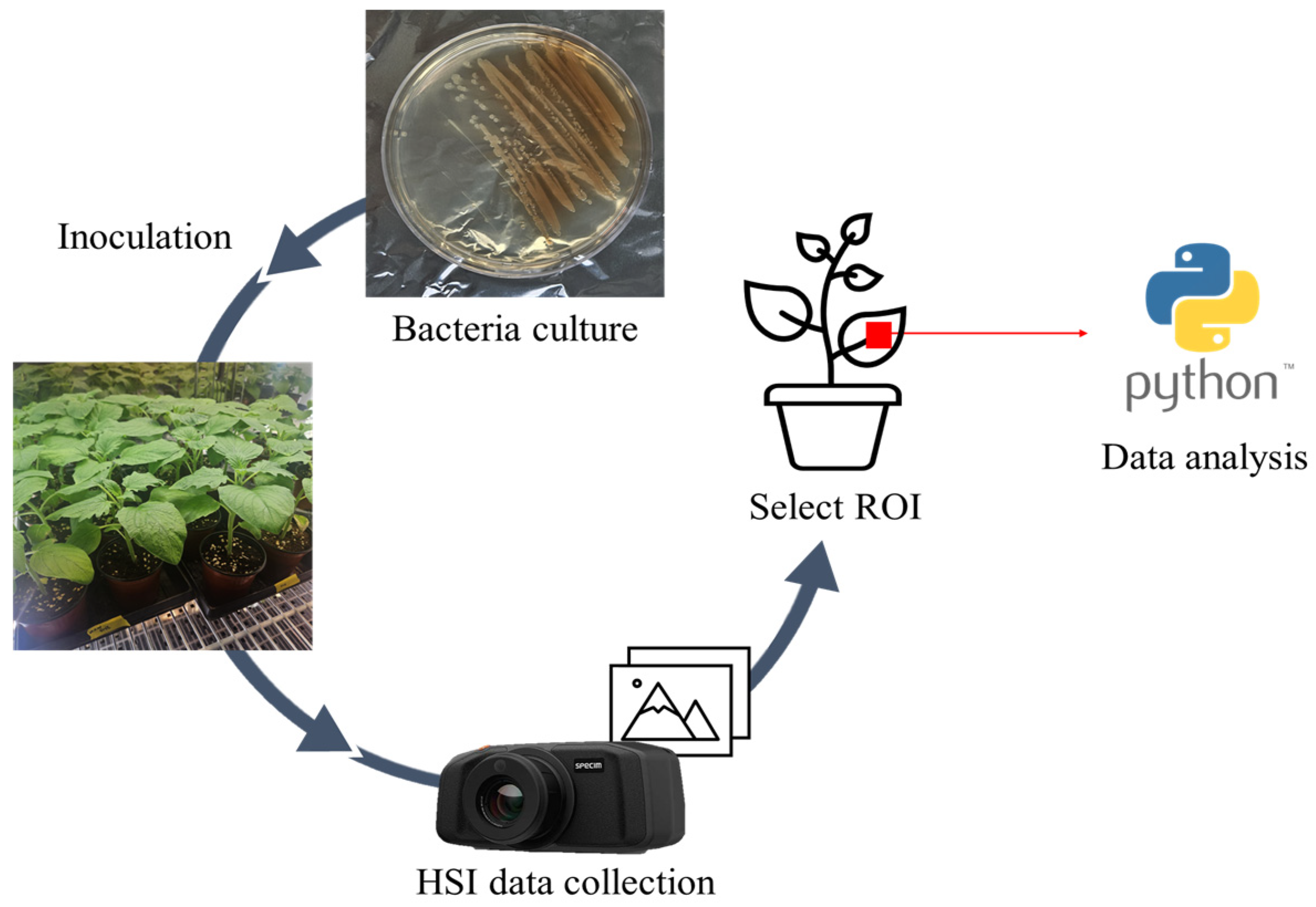
2.1. Plant Preparation and Hyperspectral Imaging

In this study, HSI was used to enable early bacterial leaf spot disease detection in sesame. The bacterial strain used, Pseudomonas syringae pv. sesami -MR4526, was collected from the Miryang region in 2020. Sesame plants were cultivated under controlled conditions in a growth chamber (JSPG-1500C, JS Research Inc., Gongju, Republic of Korea), under 14 h of daylight at 27 °C and 10 h of darkness at 25 °C, at 70% relative humidity. After the bacterial cultures were prepared using the same growth chamber, the pathogen was artificially inoculated into plants in the treatment group. HSI data were acquired at 24 h intervals, starting from the day of inoculation. The entire experiment was repeated twice, utilizing identical plant materials, methodologies, and environmental conditions. Spectral data were extracted from the collected images and used for analysis. The overall experimental procedure is illustrated in Figure 1.

2.1.1. Plant Cultivation

The experiment was conducted using the cultivated sesame variety “Geonbaek”, donated by the National Institute of Crop Science, Rural Development Administration. Seeds were sown in trays (105-cell plug tray, Gumok, Republic of Korea) and grown for two weeks. In total, 42 healthy sesame plants were selected, transplanted into pots (10.5 cm diameter and 9.5 cm height), and then cultivated until they reached the fifth vegetative growth stage (V5), which corresponds to the developmental stage where five true leaves are fully expanded on the main stem. The soil used for the cultivation was commercial horticultural soil (No.1, Chamgrow Inc., Hongsung-gun, Republic of Korea), comprising 67% cocopeat, 12% peat moss, 8% vermiculite, 9.5% perlite, 3.2% zeolite, 0.01% biochar, 0.21% fertilizer, 0.01% dolomite, and 0.001% wetting agent. The 42 plants were equally partitioned into two groups: 21 plants in the control group (non-inoculated) and 21 plants in the treatment group (inoculated with bacteria).

2.1.2. Bacterial Inoculation

For inoculation, bacteria were cultured twice in two steps. The Pseudomonas syringae pv. sesami strain-MR4526, which was preserved at −80 °C, was initially cultured on a tryptic soy agar (TSA) medium at 30 °C for 48 h. Bacteria from this initial culture were then transferred to fresh media for a second culture. The resultant bacterial culture was suspended in sterile distilled water. A total of 500 mL of the bacterial suspension was sprayed onto the treatment group, while an equivalent volume of distilled water was sprayed onto the control group.

2.1.3. Data Acquisition

HSI was performed using the Specim IQ camera (model: WL18 MODGB, firmware version: 2019.05.31.1). This camera operates on push-broom technology and captures wavelengths ranging from 400 to 1000 nm, divided into 204 spectral bands. Data were collected from 1 day after inoculation (DAI) to 9 DAI at 24 h intervals. Image data collection was conducted in a dark room to minimize ambient light interference. Two halogen lamps (650 W each) were positioned at a 45° angle relative to the plant surface and operated at approximately 65% of their maximum brightness to provide uniform illumination. The camera was mounted on a tripod and positioned vertically 70 cm above the plant canopy to enable top–down image acquisition. Calibration was performed prior to image acquisition by adjusting the camera’s focus ring and intensity slider to highlight the white reference target with maximum orange indicators and selecting the orange-colored tile area [35]. For each image captured, a raw datacube, dark frame, and white reference were recorded. Reflectance transformation was then automatically performed using the following equation:
R e f l e c t a n c e = R a w _ d a t a D a r k W h i t e D a r k
Python(3.8.18) packages (OpenCV, ENVI) were utilized to define regions of interest (ROIs) from the images, and spectral reflectance values were extracted for analysis. In the control group, 1082 samples were established by randomly cropping ROIs of various positions and pixel sizes (ranging from 5 × 5 to 70 × 70 pixels) from the leaf regions. Each ROI included pixel coordinate information and reflectance values across the 204 spectral bands. The control group data were used to train the model. In the treatment group, plants exhibiting visible disease symptoms on the ninth DAI were selected. The same leaf area was then traced backward from the ninth DAI to the first DAI to define consistent ROIs across the time series. This allowed for the extraction of the spectral reflectance values from the same leaf region during both the asymptomatic and symptomatic stages. Spectral data were collected from a total of 16 plants in the treatment group through two replicated experiments. A total of 16 spectral samples, each corresponding to ROIs, were collected from the treatment group used for the analysis. All data extracted from the ROIs included x and y coordinates for image reconstruction, along with reflectance values across 204 spectral bands.
To enhance the model training efficiency, ten noisy bands at both spectral extremes were removed. As a result, 184 bands corresponding to the wavelength range of 426–972 nm (B11–B194) were retained. The reflectance profiles of all 184 bands we collected are shown in Figure S1A. For visualization convenience, a subset of these reflectance values is presented in Figure S1B (for original bands) and Figure S1C (for averaged bands). Both Figure S1B,C demonstrate that the reflectance trend across the bands is largely monotonic. Likewise, we also visualized the range of reflectance values for a random sample image (Figure S1D). Based on this observation, and to improve the model efficiency, we grouped four adjacent bands to reduce the 184 original bands into a total of 46 bands, which were then used for training (see Table 1 and Figure S1C for the plot of these 46 grouped bands).

2.2. Modeling Framework for Anomaly Detection

Image anomaly detection focuses on modeling the distribution of normal images and identifying instances that deviate from this distribution. Early approaches relied on handcrafted features or statistical techniques, whereas modern deep learning-based methods employ reconstruction models such as autoencoders and generative adversarial networks to learn complex spectral–spatial patterns and flag anomalies based on reconstruction or latent space errors [27,28]. In the following subsubsections, we detail the key components of our modeling framework. We begin with the base autoencoder design, followed by its enhancement through U-Net style skip connections, and conclude with the integration of attention mechanisms to improve anomaly localization.

2.2.1. Autoencoder

Autoencoders are unsupervised neural networks that learn to reconstruct input images by encoding them into a low-dimensional latent space and subsequently decoding them back to the original resolution (Figure 2) [36,37]. Formally, given an input image x R H × W × C , where R denotes the space of real numbers, and H ,   W , a n d   C represent the height, width, and the number of channels (bands) of the image, respectively, the encoder f θ produces a latent vector z R d . Here, d refers to the dimensionality of the latent space, which is a configurable parameter depending on the model design and training objectives. Then, the decoder g ϕ reconstructs the image x ^ from z, as follows:
z = f θ x , x ^ = g ϕ z .
We defined the anomaly score as the per-pixel reconstruction error between the input and its reconstruction, as analogous to the MSE loss used during training:
E r e c x = x x ^ 2 2 .

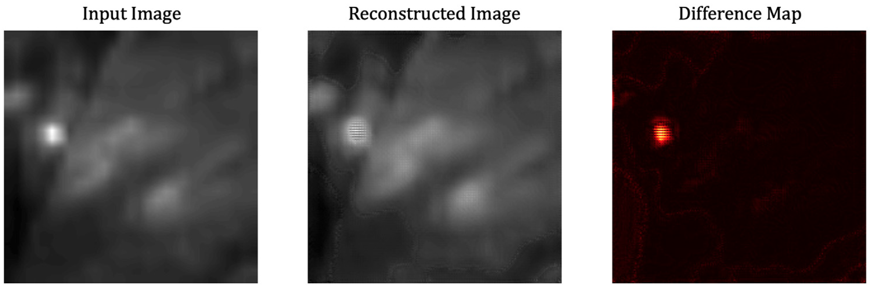
2.2.2. U-Net Based Autoencoder

The U-Net architecture, originally introduced by Ronneberger et al. (2015) [38], is a symmetric encoder–decoder framework augmented with skip connections between corresponding layers. Each encoder stage comprises two consecutive 3 × 3 convolutional layers with ReLU activations, followed by a 2 × 2 max pooling operation that reduces the spatial dimensions and increases the number of feature channels. The decoder path mirrors this structure by applying 2 × 2 transposed convolutions for upsampling, followed by two additional 3 × 3 convolutions to refine the reconstructed features.
Skip connections are used to concatenate feature maps from each encoder stage with those of the corresponding decoder stage. This design enables the transfer of fine-grained spatial information across the bottleneck, supporting the accurate reconstruction of local details.
Functionally, this encoder–skip–decoder configuration is equivalent to an autoencoder enhanced with explicit information pathways. Such a structure has been shown to be effective in anomaly detection tasks, particularly for low-resolution HSI, where precise localization of subtle spectral–spatial anomalies is required [39,40].
The autoencoder was trained exclusively on healthy plant samples, enabling it to learn normal spectral–spatial patterns; at inference, inputs yielding high reconstruction-error-based anomaly scores were flagged as anomalies [39]. Due to the limited spatial resolution of our hyperspectral data, we applied image upsampling using bilinear interpolation, which estimates pixel values by computing a weighted average of the nearest four neighboring pixels. The interpolation was implemented through torchvision. transforms. Resize(v0.21.0). To further enhance the extraction of distinctive spectral–spatial features during decoding, we integrated an attention block inspired by Oktay et al. (2018) [41], allowing the network to focus selectively on salient regions and improve anomaly localization.

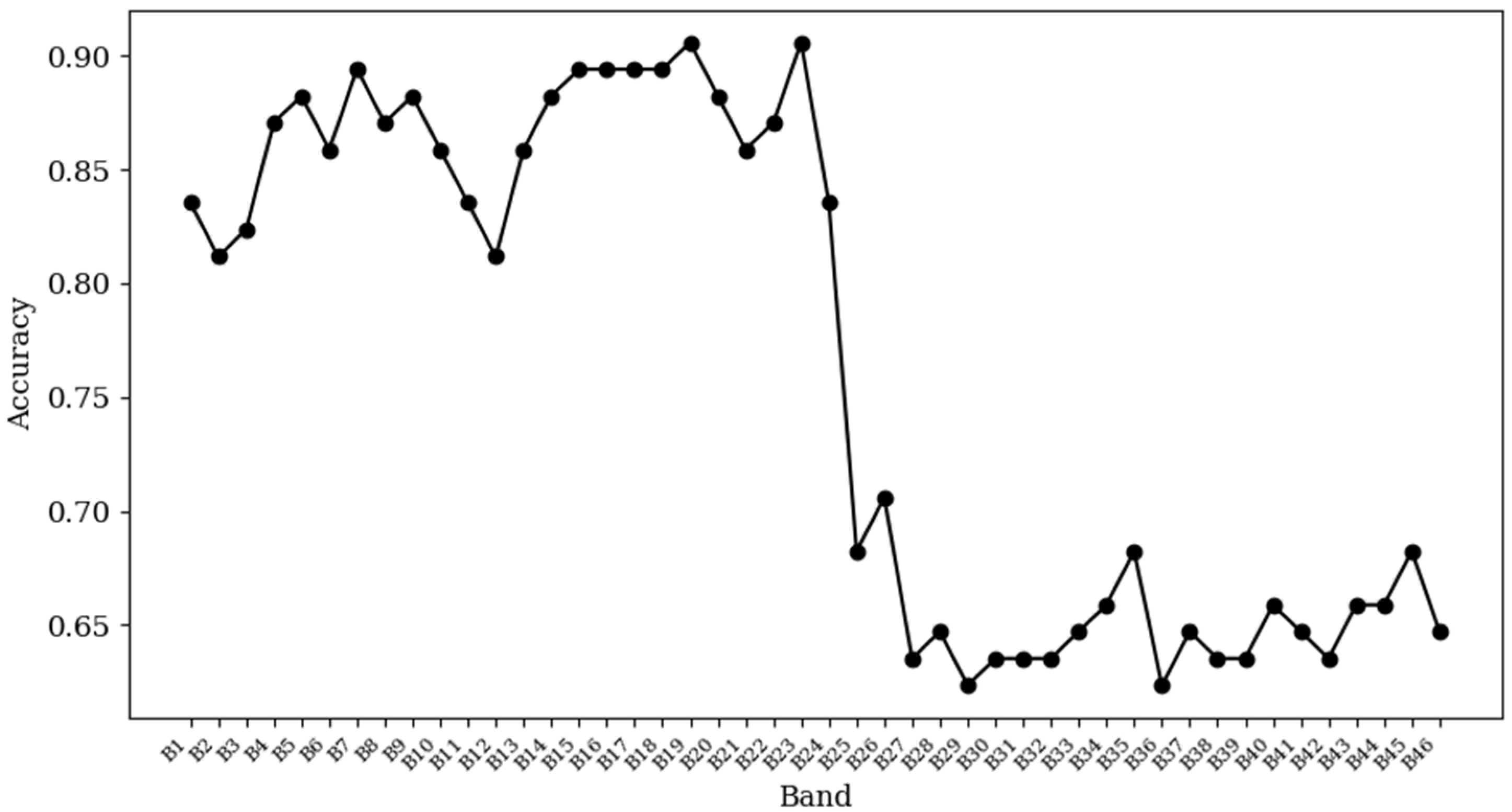
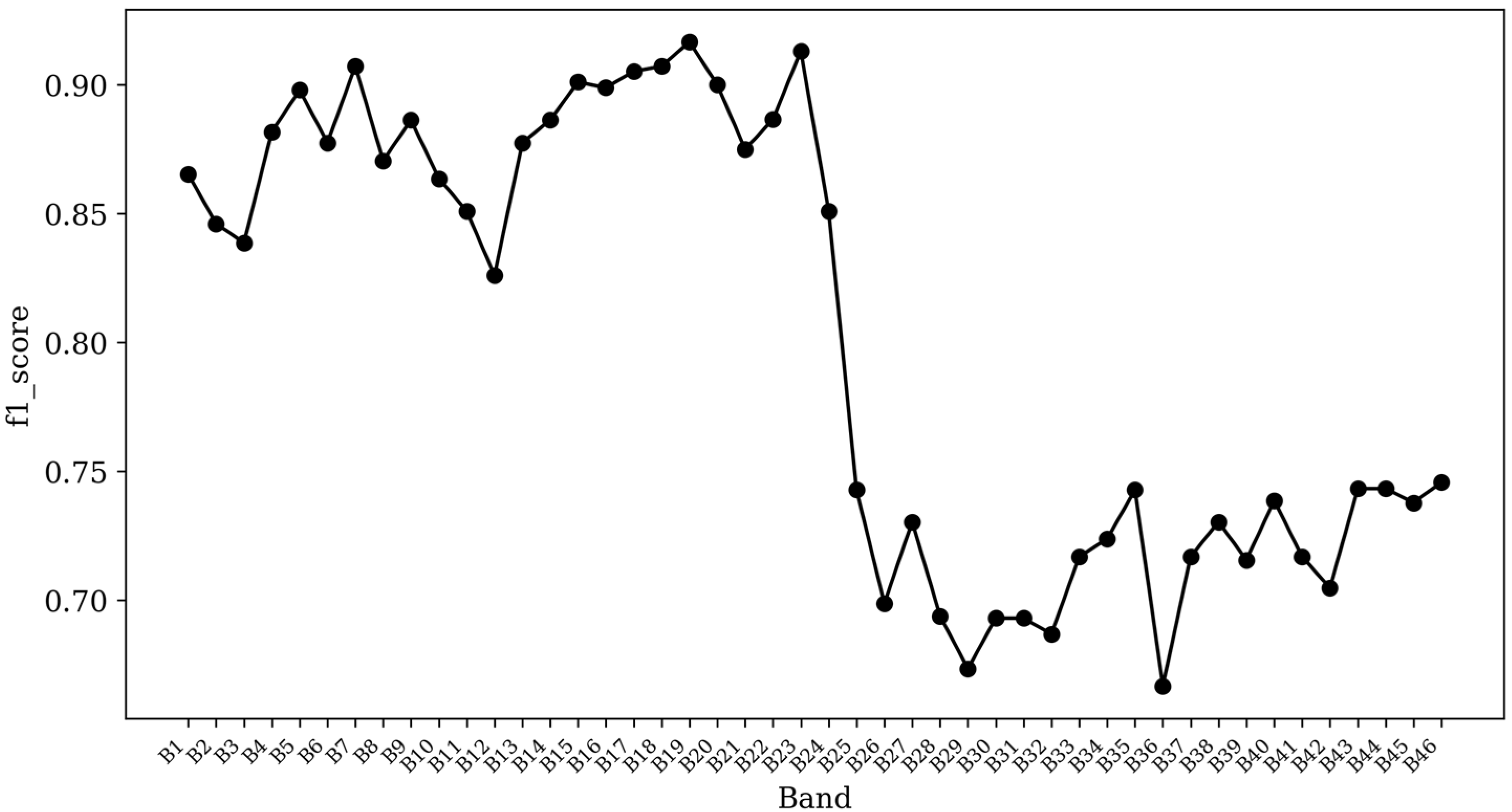
2.2.3. Model Training and Evaluation

The original HSI comprised 46 spectral bands, and to analyze spectral characteristics in a band-specific manner, each image was decomposed into 46 grayscale images corresponding to each individual band. To model the normal data distribution, our training set consisted of 1026 randomly cropped images of varying pixel sizes from healthy plant leaves (control group). These images represented the healthy plant leaves for the training phase. For evaluation, we constructed a comprehensive validation/test set. This set included 45 anomalous cropped images manually extracted from lesion areas of the Treatment group (samples 1–12), which showed visible signs of disease (labeled as 1). Additionally, this set included 40 healthy cropped images from the control group (labeled as 0) that were not used during the training phase. Due to the original images’ low spatial resolution, all cropped images were upscaled to 200 × 200 pixels using torchvision. transforms. Resize. We employed the AdamW optimizer for model training and utilized the mean-squared error loss instead of the binary cross-entropy with logits loss, which is more commonly used for binary classification. This choice aligns the training objective directly with the anomaly score metric and facilitates future optimizations toward early detection. At the inference time, the model reconstructs the input image, generating a pixel-wise difference map that highlights anomalous regions between the input and reconstructed images (Figure 3). The classification threshold was selected to maximize accuracy on the validation set, and the training was run for up to 200 epochs with early stopping to prevent overfitting. Finally, we employed Optuna, a framework for Bayesian hyperparameter optimization [42], to conduct 30 trials and tune the learning rate and weight decay parameters. The overall pipeline of the study is illustrated in Algorithm 1.
Algorithm 1: Band-wise preprocessing of hyperspectral images
  • Step 1: Band Separation Input:
  • Hyperspectral images {Ii}, each of size W × H × B
  • (In this study, B = 46)
  • Output: Band-separated grayscale images {Gi,b} Details:
    • For each hyperspectral image Ii, extract all B spectral bands.
    • Store each band b as a 2D grayscale image Gi,b.
  • Step 2: Normal Pattern Learning
  • Input: {Gi,b} from Control group
  • Output: — (No direct output)
  • Details:
    • For each band b, train an autoencoder using only Control group images.
    • The model captures normal reconstruction patterns for each spectral band.
  • Step 3: Binary Classification and Evaluation Input:
  • {Gi,b} from the Treatment group as label 1,
  • {Gi,b} from the unused Control group as label 0
  • Output: Best model, best parameters, accuracy, threshold, difference map. Details:
    • For each band b, compute the reconstruction error using the trained model.
    • Train a binary classifier (label 1: Treatment, label 0: unused Control).
    • Use Optuna to tune training hyperparameters (e.g., learning rate).
    • Determine the threshold that maximizes Accuracy on the validation set.
    • Save the best model, best parameters, accuracy, and difference map.

3. Results

In this study, we applied the U-Net-based autoencoder for anomaly detection in HSI data of sesame plants from the Treatment group (plants inoculated with Pseudomonas syringae pv. sesami) and the control group.
Based on the aforementioned procedures, we computed the classification accuracy (Figure 4 and Table S1) and f1-score (Figure 5 and Table S2) for each spectral band. A substantial shift in accuracy was observed around Band 24, which approximately corresponds to the boundary between the visible (VIS) and near-infrared (NIR) spectral regions. Our analysis revealed consistently higher accuracy in the VIS range, particularly with Band B19 and Band B23, achieving an accuracy of 0.90 and representing the highest classification performance. Therefore, B19 and B23 (with wavelengths of 641 nm and 689 nm) can be used to detect bacterial leaf spot in sesame. In contrast, the classification accuracy drops sharply at B24. The region corresponding to B24–B46 (701–968 nm) belongs to the near-infrared region and shows a low classification accuracy of about 0.6~0.7. Similar results were obtained in the case of the f1-score, where a higher f1-score > 0.90 was obtained for B19 and B23, and a sharp decline in value was observed starting from B24 (similar to the accuracy result).

4. Discussion

This study employed hyperspectral imaging (HSI) in conjunction with an autoencoder-based anomaly detection method to detect bacterial leaf spot in sesame. Following the anomaly score generation, classification was performed to distinguish healthy and symptomatic samples. Band-wise evaluation of the classification accuracy indicated that bands within the visible spectrum (430–689 nm) achieved relatively high performance, with accuracy exceeding 0.8. In particular, the highest classification accuracy was observed at 641 nm and 689 nm, respectively, corresponding to the red and red-edge regions. In contrast, the classification accuracy markedly declined in wavelengths exceeding 700 nm. Previous studies have reported that Pseudomonas syringae produces toxins such as coronatine [43], and other secondary metabolites within host tissues, causing structural damage to cell walls and chlorophyll, which results in chlorosis [8,44]. Moreover, phytotoxins produced by Pseudomonas syringae can suppress chlorophyll biosynthesis or activate chlorophyll-degrading enzymes, thereby reducing the overall chlorophyll content [44]. These changes in the chlorophyll fluorescence affect light absorption and scattering in plant tissues [45]. The superior classification performance in the red and red-edge regions observed in this study can be attributed to color-based alterations resulting from chlorophyll degradation, which significantly affect the spectral reflectance. In particular, the red-edge region is well known for its high sensitivity to variations in the chlorophyll concentration [46] and has been reported to be effective for the early detection of plant stress [47].
A sharp decline in the classification performance was observed in the near-infrared region above 700 nm, presumably due to the reflectance in this range being more influenced by the cell structure and water content than pigments such as chlorophyll [48,49]. Since the infections at the early growth stage investigated in this study are primarily associated with chloroplast damage, the visible red region was more sensitive for disease detection. Therefore, selecting wavelengths responsive to infection, such as the 641 nm and 689 nm identified in this study, may improve the classification performance and enhance the model interpretability and dimensionality reduction.
Since the model was trained only on healthy samples, it has limitations in distinguishing between different types of biotic and abiotic stress. As a result, the anomaly scores generated for new samples may not be exclusively indicative of bacterial leaf spot. However, this study identified specific wavelength regions that consistently responded to bacterial leaf spot symptoms. Despite the many advantages of hyperspectral imaging, the high cost limits its practicality for field applications [25]. To address this, selecting stress-responsive wavelength regions can be an effective alternative [50]. The wavelengths identified in this study may serve as a basis for developing targeted multispectral sensors suitable for field use. This approach can also be useful for identifying specific wavelengths responsive to a particular stress, especially when the number of lesion samples is limited but symptoms are clearly distinguishable.
Furthermore, the difference map facilitates the assessment of the model’s efficacy in accurately capturing and defining lesion areas. This provides a qualitative assessment that goes beyond numerical metrics, such as accuracy, particularly in studies like ours that rely on individual-level comparisons across spectral bands. One of the primary goals of this study was early prediction, enabled by the time-series nature of HSI data collected in a non-destructive manner. As shown in Figure 6, the model demonstrated potential for early detection across specific spectral bands and test samples. However, the performance was not consistent across all bands and samples, complicating the generalization of the results. This limitation is related to the nature of the deep learning-based approach adopted in this study, which typically requires a large amount of training data. However, in our case, the available data were limited due to (i) the utilization of living organisms in our study and (ii) the difficulty of inducing biotic stress in the target plant. Despite these experimental challenges, we plan to expand the dataset through additional experiments and explore the use of alternative methodologies with a stronger focus on early detection in future research.

5. Conclusions

Timely detection of the disease incidence in any crop can prevent severe yield and productivity losses. In this study, we classified the bacterial leaf spot disease in sesame based on an anomaly detection method. Hyperspectral imaging combined with a U-Net-based autoencoder classified the diseased and non-diseased plants with an average accuracy of >0.8 within the 430–701 nm wavelength range. Furthermore, two specific wavelengths (641 nm and 689 nm) exhibited peak accuracy percentages exceeding 0.9. This study confirms that spectral imaging when integrated with deep learning methods can be the best alternative to the traditional methods of disease detection and classification at an early stage. The specified methodology also presents potential for scalable, non-destructive field applications. Nonetheless, extensive research remains necessary to establish correlations between specific wavelengths with specific diseases and to validate the method across varying environmental and crop conditions.

Supplementary Materials

The following supporting information can be downloaded at: https://www.mdpi.com/article/10.3390/rs17132230/s1.

Author Contributions

Conceptualization, Y.K.; methodology, M.L. and J.L.; software, J.L.; validation, Y.K. and B.K.; formal analysis, J.L.; investigation, M.L., A.G., and Y.B.; resources, Y.K., Y.Y., and T.-A.K.; data curation, M.L.; writing—original draft preparation, M.L. and J.L.; writing—review and editing, Y.K., A.G., and B.K.; visualization, J.L., M.L.; supervision, Y.K.; project administration, Y.K.; funding acquisition, Y.K.; I.-J.L. and C.-W.P. All authors have read and agreed to the published version of the manuscript.

Funding

This work was supported by the Commercialization Promotion Agency for R&D Outcomes (COMPA) grant funded by the Korean Government (Ministry of Science and ICT), (RS-2023-00304695) and in part by the Korea Research Foundations, Korea, under grant RS-2023-00213626. The funders had no role in study design, data collection and analysis, decision to publish, or preparation of the manuscript.

Data Availability Statement

The original contributions presented in this study are included in the article. Further inquiries can be directed to the corresponding authors. The code, trained models, experimental results and list of packages and versions used in this study are publicly available at https://github.com/dlakakwns/U-Net-autoencoder-Sesame.git (accessed on 26 June 2025).

Conflicts of Interest

The authors declare no conflicts of interest.

References

  1. Faostat. Crops and Livestock Products-Production Quantity of Sesame Seeds; Food and Agriculture Organization of the United Nations: Rome, Italy, 2023. [Google Scholar]
  2. Namiki, M. Nutraceutical functions of sesame: A review. Crit. Rev. Food Sci. Nutr. 2007, 47, 651–673. [Google Scholar] [CrossRef] [PubMed]
  3. Jyothi, B.; Ansari, N.A.; Vijay, Y.; Anuradha, G.; Sarkar, A.; Sudhakar, R.; Siddiq, E. Assessment of resistance to Fusarium wilt disease in sesame (Sesamum indicum L.) germplasm. Austalas. Plant Pathol. 2011, 40, 471–475. [Google Scholar] [CrossRef]
  4. Ransingh, N.; Khamari, B.; Adhikary, N. Modern approaches for management of sesame diseases. In Innovative Approaches in Diagnosis and Management of Crop Diseases; Apple Academic Press: Palm Bay, FL, USA, 2021; pp. 123–162. [Google Scholar]
  5. Vajavat, R.; Chakravarti, B. Yield Losses due to Bacterial Leaf Spot of Sesamum Orientale in Rajasthan; CABI: Wallingford, UK, 1977. [Google Scholar]
  6. Prathuangwong, S.; Yowabutra, P. Effects of bacterial leaf spot on yield, resistance, and seedborne infection of sesame in Thailand. In Pseudomonas Syringae Pathovars and Related Pathogens; Springer: Berlin/Heidelberg, Germany, 1997; pp. 53–60. [Google Scholar]
  7. Langham, D.; Cochran, K. Fungi, Oomycetes, Bacteria, and Viruses Associated with Sesame (Sesamum indicum L.); Sesame Research; LLCR&D: San Antonio, TX, USA, 2021. [Google Scholar]
  8. Firdous, S.S.; Asghar, R.; Ul-Haque, M.I.; Waheed, A.; Afzal, S.N.; Mirza, M.Y. Pathogenesis of Pseudomonas syringae pv. sesami associated with Sesame (Sesamum indicum L.) bacterial leaf spot. Pak. J. Bot. 2009, 41, 927–934. [Google Scholar]
  9. Fang, Y.; Ramasamy, R.P. Current and prospective methods for plant disease detection. Biosensors 2015, 5, 537–561. [Google Scholar] [CrossRef]
  10. Alemu, K. Detection of diseases, identification and diversity of viruses. J. Biol. Agric. Healthc. 2015, 5, 204–213. [Google Scholar]
  11. Donoso, A.; Valenzuela, S. In-field molecular diagnosis of plant pathogens: Recent trends and future perspectives. Plant Pathol. 2018, 67, 1451–1461. [Google Scholar] [CrossRef]
  12. Farber, C.; Mahnke, M.; Sanchez, L.; Kurouski, D. Advanced spectroscopic techniques for plant disease diagnostics. A review. Trends Anal. Chem. 2019, 118, 43–49. [Google Scholar] [CrossRef]
  13. Sankaran, S.; Mishra, A.; Ehsani, R.; Davis, C. A review of advanced techniques for detecting plant diseases. Comput. Electron. Agric. 2010, 72, 1–13. [Google Scholar] [CrossRef]
  14. Li, S.; Song, W.; Fang, L.; Chen, Y.; Ghamisi, P.; Benediktsson, J.A. Deep learning for hyperspectral image classification: An overview. IEEE Trans. Geosci. Remote Sens. 2019, 57, 6690–6709. [Google Scholar] [CrossRef]
  15. Keshava, N. A survey of spectral unmixing algorithms. Linc. Lab. J. 2003, 14, 55–78. [Google Scholar]
  16. Shaw, G.A.; Burke, H.K. Spectral imaging for remote sensing. Linc. Lab. J. 2003, 14, 3–28. [Google Scholar]
  17. Li, Q.; He, X.; Wang, Y.; Liu, H.; Xu, D.; Guo, F. Review of spectral imaging technology in biomedical engineering: Achievements and challenges. J. Biomed. Opt. 2013, 18, 100901. [Google Scholar] [CrossRef]
  18. Zhang, Q.; Luan, R.; Wang, M.; Zhang, J.; Yu, F.; Ping, Y.; Qiu, L. Research Progress of Spectral Imaging Techniques in Plant Phenotype Studies. Plants 2024, 13, 3088. [Google Scholar] [CrossRef] [PubMed]
  19. Kuswidiyanto, L.W.; Noh, H.-H.; Han, X. Plant disease diagnosis using deep learning based on aerial hyperspectral images: A review. Remote Sens. 2022, 14, 6031. [Google Scholar] [CrossRef]
  20. Wan, L.; Li, H.; Li, C.; Wang, A.; Yang, Y.; Wang, P. Hyperspectral sensing of plant diseases: Principle and methods. Agronomy 2022, 12, 1451. [Google Scholar] [CrossRef]
  21. García-Vera, Y.E.; Polochè-Arango, A.; Mendivelso-Fajardo, C.A.; Gutiérrez-Bernal, F.J. Hyperspectral image analysis and machine learning techniques for crop disease detection and identification: A review. Sustainability 2024, 16, 6064. [Google Scholar] [CrossRef]
  22. Ravikanth, L.; Jayas, D.S.; White, N.D.; Fields, P.G.; Sun, D.-W. Extraction of spectral information from hyperspectral data and application of hyperspectral imaging for food and agricultural products. Food Bioprocess Technol. 2017, 10, 1–33. [Google Scholar] [CrossRef]
  23. Mahesh, S.; Jayas, D.; Paliwal, J.; White, N. Hyperspectral imaging to classify and monitor quality of agricultural materials. J. Stored Prod. Res. 2015, 61, 17–26. [Google Scholar] [CrossRef]
  24. Kumar, B.; Dikshit, O.; Gupta, A.; Singh, M.K. Feature extraction for hyperspectral image classification: A review. Int. J. Remote Sens. 2020, 41, 6248–6287. [Google Scholar] [CrossRef]
  25. Matese, A.; Czarnecki, J.M.P.; Samiappan, S.; Moorhead, R. Are unmanned aerial vehicle-based hyperspectral imaging and machine learning advancing crop science? Trends Plant Sci. 2024, 29, 196–209. [Google Scholar] [CrossRef]
  26. Chandola, V.; Banerjee, A.; Kumar, V. Anomaly detection: A survey. ACM Comput. Surv. 2009, 41, 1–58. [Google Scholar] [CrossRef]
  27. Pang, G.; Shen, C.; Cao, L.; Hengel, A.V.D. Deep learning for anomaly detection: A review. ACM Comput. Surv. 2021, 54, 1–38. [Google Scholar] [CrossRef]
  28. Schlegl, T.; Seeböck, P.; Waldstein, S.M.; Schmidt-Erfurth, U.; Langs, G. Unsupervised Anomaly Detection with Generative Adversarial Networks to Guide Marker Discovery. In Proceedings of the International Conference on Information Processing in Medical Imaging, Boone, NC, USA, 25–30 June 2017; pp. 146–157. [Google Scholar]
  29. Schlegl, T.; Seeböck, P.; Waldstein, S.M.; Langs, G.; Schmidt-Erfurth, U. f-AnoGAN: Fast unsupervised anomaly detection with generative adversarial networks. Med. Image Anal. 2019, 54, 30–44. [Google Scholar] [CrossRef] [PubMed]
  30. Cheshkova, A. A review of hyperspectral image analysis techniques for plant disease detection and identif ication. Vavilovsk. Zhurn. Genet. Selekts. 2022, 26, 202. [Google Scholar] [CrossRef]
  31. Zhang, J.; Huang, Y.; Pu, R.; Gonzalez-Moreno, P.; Yuan, L.; Wu, K.; Huang, W. Monitoring plant diseases and pests through remote sensing technology: A review. Comput. Electron. Agric. 2019, 165, 104943. [Google Scholar] [CrossRef]
  32. Khan, A.; Sohail, A.; Zahoora, U.; Qureshi, A.S. A survey of the recent architectures of deep convolutional neural networks. Artif. Intell. Rev. 2020, 53, 5455–5516. [Google Scholar] [CrossRef]
  33. Ma, L.; Liu, Y.; Zhang, X.; Ye, Y.; Yin, G.; Johnson, B.A. Deep learning in remote sensing applications: A meta-analysis and review. ISPRS J. Photogramm. Remote Sens. 2019, 152, 166–177. [Google Scholar] [CrossRef]
  34. Freeman, E.A.; Moisen, G.G. A comparison of the performance of threshold criteria for binary classification in terms of predicted prevalence and kappa. Ecol. Model. 2008, 217, 48–58. [Google Scholar] [CrossRef]
  35. Lay, L.; Lee, H.S.; Tayade, R.; Ghimire, A.; Chung, Y.S.; Yoon, Y.; Kim, Y. Evaluation of soybean wildfire prediction via hyperspectral imaging. Plants 2023, 12, 901. [Google Scholar] [CrossRef]
  36. Vincent, P.; Larochelle, H.; Bengio, Y.; Manzagol, P.-A. Extracting and composing robust features with denoising autoencoders. In Proceedings of the Proceedings of the 25th International Conference on Machine Learning, Helsinki, Finland, 5–9 July 2008; pp. 1096–1103. [Google Scholar]
  37. Rumelhart, D.E.; Hinton, G.E.; Williams, R.J. Learning representations by back-propagating errors. Nature 1986, 323, 533–536. [Google Scholar] [CrossRef]
  38. Ronneberger, O.; Fischer, P.; Brox, T. U-net: Convolutional networks for biomedical image segmentation. In Proceedings of the Medical Image Computing and Computer-Assisted Intervention–MICCAI 2015: 18th International Conference, Munich, Germany, 5–9 October 2015; part III 18, pp. 234–241. [Google Scholar]
  39. Sakurada, M.; Yairi, T. Anomaly detection using autoencoders with nonlinear dimensionality reduction. In Proceedings of Proceedings of the MLSDA 2014 2nd Workshop on Machine Learning for Sensory Data Analysis, Gold Coast, Australia, 2 December 2014; pp. 4–11. [Google Scholar]
  40. Mao, X.; Shen, C.; Yang, Y.-B. Image restoration using very deep convolutional encoder-decoder networks with symmetric skip connections. Adv. Neural Inf. Process. Syst. 2016, 29, 2810–2818. [Google Scholar]
  41. Oktay, O.; Schlemper, J.; Folgoc, L.L.; Lee, M.; Heinrich, M.; Misawa, K.; Mori, K.; McDonagh, S.; Hammerla, N.Y.; Kainz, B. Attention u-net: Learning where to look for the pancreas. arXiv 2018, arXiv:1804.03999. [Google Scholar]
  42. Akiba, T.; Sano, S.; Yanase, T.; Ohta, T.; Koyama, M. Optuna: A next-generation hyperparameter optimization framework. In Proceedings of the Proceedings of the 25th ACM SIGKDD International Conference on Knowledge Discovery & Data Mining, Anchorage, AK, USA, 4–8 August 2019; pp. 2623–2631. [Google Scholar]
  43. Fardoos, S. Virulence Analysis of Xanthomonas Campestris Pv. Sesami and Pseudomonas Syringae Pv. Sesami the Causal Organisms of Sesame (Sesamum indicum L.) Bacterial Blight; Arid Agriculture University Rawalpindi: Pothohar Plateau, Pakistan, 2009. [Google Scholar]
  44. Bender, C.L. Chlorosis-inducing phytotoxins produced by Pseudomonas syringae. Eur. J. Plant Pathol. 1999, 105, 1–12. [Google Scholar] [CrossRef]
  45. Zhang, Z.; He, B.; Sun, S.; Zhang, X.; Li, T.; Wang, H.; Xu, L.; Afzal, A.J.; Geng, X. The phytotoxin COR induces transcriptional reprogramming of photosynthetic, hormonal and defence networks in tomato. Plant Biol. 2021, 23, 69–79. [Google Scholar] [CrossRef] [PubMed]
  46. Carter, G.A.; Knapp, A.K. Leaf optical properties in higher plants: Linking spectral characteristics to stress and chlorophyll concentration. Am. J. Bot. 2001, 88, 677–684. [Google Scholar] [CrossRef]
  47. Horler, D.; Dockray, M.; Barber, J. The red edge of plant leaf reflectance. Int. J. Remote Sens. 1983, 4, 273–288. [Google Scholar] [CrossRef]
  48. Peñuelas, J.; Filella, I.; Biel, C.; Serrano, L.; Save, R. The reflectance at the 950–970 nm region as an indicator of plant water status. Int. J. Remote Sens. 1993, 14, 1887–1905. [Google Scholar] [CrossRef]
  49. Peñuelas, J.; Filella, I. Visible and near-infrared reflectance techniques for diagnosing plant physiological status. Trends Plant Sci. 1998, 3, 151–156. [Google Scholar] [CrossRef]
  50. Hunt, E.R., Jr.; Daughtry, C.S. What good are unmanned aircraft systems for agricultural remote sensing and precision agriculture? Int. J. Remote Sens. 2018, 39, 5345–5376. [Google Scholar] [CrossRef]
Figure 1. Schematic overview of the bacterial inoculation and data acquisition and analysis procedures.
Remotesensing 17 02230 g001
Figure 2. Depiction of a standard autoencoder architecture, where the encoder compresses input images into a low-dimensional latent space and the decoder reconstructs the original inputs. The reconstruction error is used as an anomaly score for detecting abnormal patterns.
Remotesensing 17 02230 g002
Figure 3. Pixel-wise difference maps generated during the anomaly detection process. From left to right: the upscaled input image (200 × 200 pixels), the reconstructed image produced by the U-Net-based autoencoder, and the pixel-wise difference map computed between the input and reconstructed images. Bright regions in the difference map indicate areas with large reconstruction errors, suggesting potential anomalies.
Remotesensing 17 02230 g003
Figure 4. The classification accuracy for each spectral band. Bands B1 to B24, which correspond to the visible spectrum, demonstrate a relatively high classification performance with accuracy exceeding 0.8. In contrast, bands B25 to B46, corresponding to the near-infrared spectrum, exhibit lower performance, with accuracy levels of around 0.6. Detailed accuracy values for each band are provided in Table S1.
Remotesensing 17 02230 g004
Figure 5. The classification f1-score for each spectral band. Bands B1 to B24, which correspond to the visible spectrum, demonstrate relatively high classification performance, with the f1-score exceeding 0.8. In contrast, bands B25 to B46, corresponding to the near-infrared spectrum, exhibit lower performance, with f1-score levels of around 0.6. Detailed f1-score values for each band are provided in Table S2.
Remotesensing 17 02230 g005
Figure 6. Anomaly scores over time for Sample 15 in band 22. The green line represents the anomaly scores, and the red dashed line indicates the threshold. Since disease symptoms tend to progress over time, the anomaly scores exhibit a monotonic increasing trend. A visible lesion was observed on Day 6 (index: 5), while the anomaly score had already exceeded the threshold on Day 5 (index: 4). This suggests that the sample had likely entered the symptomatic stage by Day 5, even in the absence of visible signs.
Remotesensing 17 02230 g006
Table 1. Band and wavelength mapping of hyperspectral channels. Wavelengths were represented by the average of the wavelength values of four consecutive bands.
BandWavelength (nm)BandWavelength (nm)BandWavelength (nm)BandWavelength (nm)
B1430.53B13570.60B25713.06B37857.90
B2442.11B14582.38B26725.03B38870.07
B3453.71B15594.18B27737.03B39882.27
B4465.32B16605.99B28749.04B40894.48
B5476.96B17617.82B29761.07B41906.71
B6488.59B18629.67B30773.12B42918.95
B7500.26B19641.53B31785.18B43931.21
B8511.94B20653.41B32797.26B44943.49
B9523.64B21665.30B33809.35B45955.78
B10535.36B22677.22B34821.47B46968.09
B11547.09B23689.15B35833.59
B12558.83B24701.09B36845.74
Disclaimer/Publisher’s Note: The statements, opinions and data contained in all publications are solely those of the individual author(s) and contributor(s) and not of MDPI and/or the editor(s). MDPI and/or the editor(s) disclaim responsibility for any injury to people or property resulting from any ideas, methods, instructions or products referred to in the content.

