Enhanced Detection of Permafrost Deformation with Machine Learning and Interferometric SAR Along the Qinghai–Tibet Engineering Corridor

Abstract

Interferometric synthetic aperture radar (InSAR) plays a significant role in monitoring permafrost deformation. However, owing to environmental constraints in permafrost regions, some regions exhibit temporal incoherence, which results in deformation with fewer measurement points and difficulties with deformation automatic detection. In this study, a full-coverage deformation rate map of the 10 km buffer of the Qinghai–Tibet Engineering Corridor (QTEC) was generated by combining nine driving factors and the deformation rate of the 5 km buffer along the QTEC based on three machine learning methods. The importance of the factors contributing to ground deformation was explored. The experimental results show that support vector regression (SVR) yielded the best performance (R2 = 0.98, RMSE = 0.76 mm/year, MAE = 0.74 mm/year). The 10 km buffer of deformation data obtained not only preserved the original deformation data well, but it also filled the blank areas in the deformation map. Subsequently, we trained the Faster R-CNN model on the deformation rate map simulated by SVR and used it for the automatic detection of permafrost thaw settlement areas. The results showed that the Faster R-CNN could identify the permafrost thawing slump quickly and accurately. More than 300 deformation areas along the QTEC were detected through our proposed method, with some of these areas located near thaw slump and thermokarst lake regions. This study confirms the significant potential of combining InSAR and deep learning techniques for permafrost degradation monitoring applications.

1. Introduction

Permafrost is an important component of the cryosphere [1] that is sensitive to climate change. Currently, permafrost is warming, leading to serious permafrost geo-hazards, such as thaw slumping and thermokarst subsidence. Permafrost thaw settlement has a significant impact on the cryosphere, posing substantial potential risks to infrastructure and human security [1]. Research indicates that 30–50% of the infrastructure in the Arctic and high-altitude areas will be in a high-risk state by 2050 [2,3,4]. In the Qinghai–Tibet Plateau region, approximately 30% of the damage to engineering infrastructure (e.g., the Qinghai–Tibet Railway) is attributed to permafrost degradation [5]. Therefore, it is important to detect potential permafrost degradation areas of the QTP.

Conventional techniques, such as leveling and the Global Navigation Satellite System (GNSS), can be utilized to monitor ground motion with high accuracy. However, these methods suffer from some limitations, such as the consumption of large amounts of human and material resources and low efficiency when conducting large-scale surveys [6]. Interferometric synthetic aperture radar (InSAR) can monitor ground deformation information by utilizing the interferometric phase [7,8]. InSAR has been widely applied to studying permafrost thaw monitoring in the past two decades [9,10,11]. Nevertheless, as an indirect remote sensing technique, InSAR measurements are subject to uncertainties caused by atmospheric delays, temporal decorrelation, and topographic effects [12,13,14]. To improve reliability, recent studies have highlighted the benefits of integrating InSAR with direct measurements (e.g., GNSS or ground sensors) for calibration and validation [15,16]. Permafrost thawing-related ground deformation derived from InSAR can be used for detecting retrogressive thaw slumps (RTSs). Jiao et al. (2023) [17] utilized InSAR deformation, optical images, and the normalized difference vegetation index (NDVI) to map the spatiotemporal variation characteristics of RTSs. Zhang et al. (2023) [18] jointly employed multisource feature data to automatically map thaw slump landforms in the Beilu River Basin of the QTP.

While InSAR provides high-resolution deformation measurements, interpreting large-scale InSAR datasets—especially in permafrost regions with complex noise patterns—remains challenging because of the need for manual intervention and expert knowledge. Recently, deep learning (DL) has demonstrated impressive performance in the fields of object detection and achieved region-based target monitoring using remote sensing imagery [19]. Several studies have integrated DL and optical images for RTS detection and achieved promising results in recent years [19,20,21]. For example, Huang et al. (2020) [22] mapped the RTSs in the Beiluhe region using DeepLabv3+ and CubeSat images. Yang et al. (2023) [23] utilized deep neural network models to map RTSs across various terrains in Siberia and Canada. These studies provided valuable insights into the investigation of RTSs. Researchers have begun to use DL and InSAR for automatic subsidence detection applications [24,25,26,27,28]. These achievements in different domains confirm the potential of deep learning for automatically identifying deformation areas from InSAR data. However, the environmental conditions in the permafrost region of the QTP are unique, and there may be poor results or even blank areas in the deformation results of regions with low coherence, thereby affecting the detection results. Furthermore, automatic detection methods for permafrost degradation areas based on InSAR results are still lacking.

In this study, a comprehensive framework for simulating large-scale permafrost thaw deformation and its automatic detection by combining InSAR and machine learning is proposed. We employed InSAR and machine learning techniques to predict the deformation rate within a 10 km buffer zone along the permafrost engineering corridor in the QTP. Additionally, we explored the contributions of different factors to permafrost deformation. Building on this, we utilized a deep learning model to identify potential permafrost thaw settlement regions. The proposed model was expanded to the other permafrost regions.

2. Study Area and Datasets

2.1. Study Area

The permafrost region of the Qinghai–Tibet Engineering Corridor (QTEC), a critical infrastructure zone encompassing the Qinghai–Tibet Railway and Highway, stretching from Anduo to Xidatan, was selected as the study site, as shown in Figure 1a,b. The QTEC is located at the center of the QTP, with a length of 1100 km from Golmud to Lhasa and a width of 10 km [29]. Several significant permafrost infrastructures, such as the Qinghai–Tibet Railway and Highway, oil pipelines, and electric transmission lines, have been constructed in the QTEC (Figure 1) [30]. More than half of the study area is in warm permafrost regions, and over 20% of the study area is in high-temperature and ice-rich regions [31]. The mean annual ground temperature (MAGT) along the Beiluhe–Kaixinling and Anduo–Xidatan transects exhibits significantly higher values compared to other segments of the Qinghai–Tibet Engineering Corridor (QTEC) [32]. The temperature decreases to a monthly average of −25 °C in December and rises to a monthly average of 12 °C in July. The maximum precipitation occurs from July to September, and the annual mean precipitation exceeds 400 mm [33]. The main vegetation types are alpine meadows and deserts [34], as shown in Figure 1c,d.

2.2. Dataset

2.2.1. SAR Datasets

In this study, the free Sentinel-1A images were collected to monitor the ground motion along the QTEC. Sentinel-1A was launched by the European Space Agency (ESA) in 2014. Over 150 Sentinel-1A single-look complex (SLC) images with VV polarization and IW (Interferometric Wide) mode acquired from March 2017 to June 2018 were collected, with a temporal resolution of 12 days. The spatial resolutions in the azimuth and range directions were 20 and 5 m, respectively.

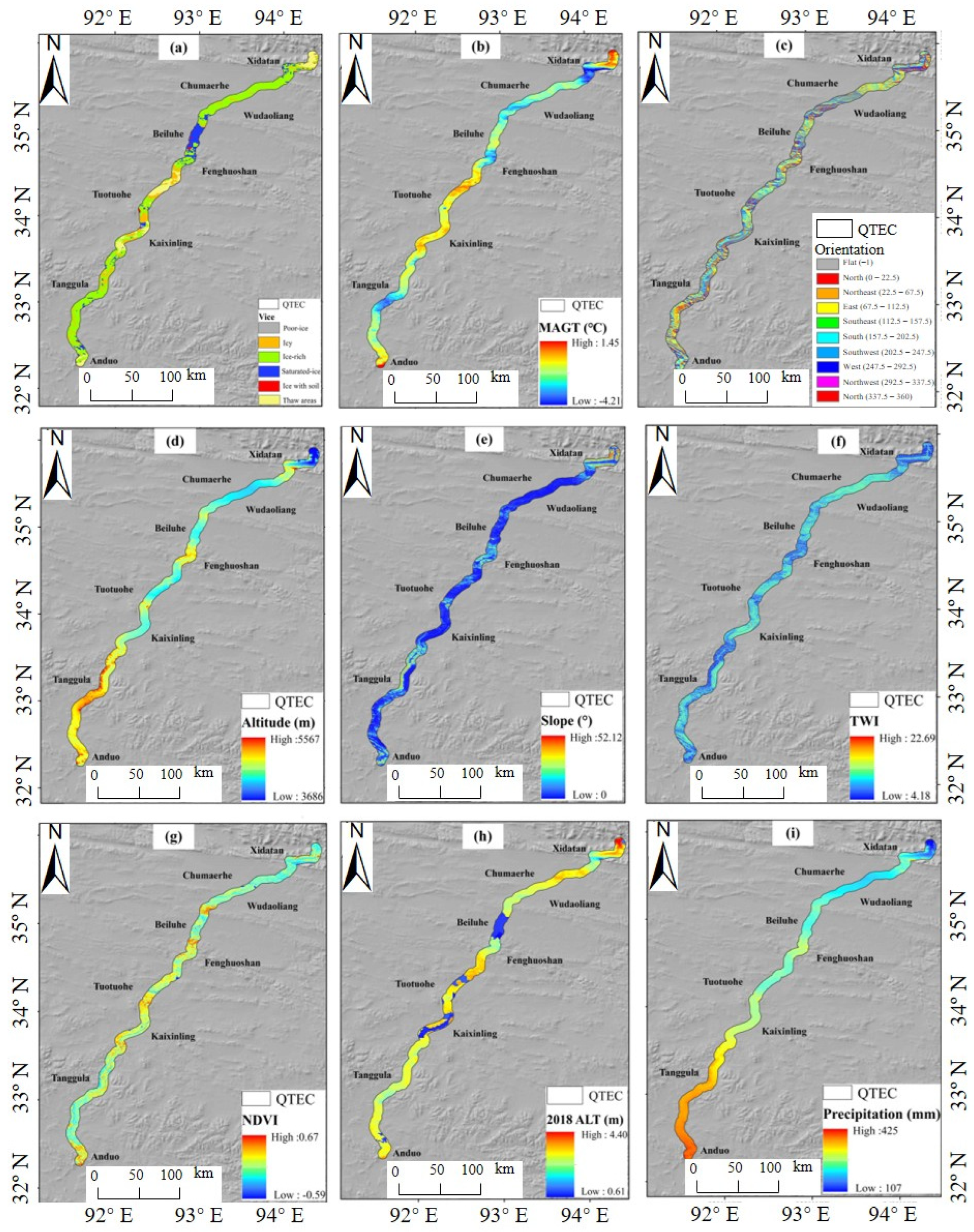
2.2.2. Factors Driving Permafrost Thaw Settlement

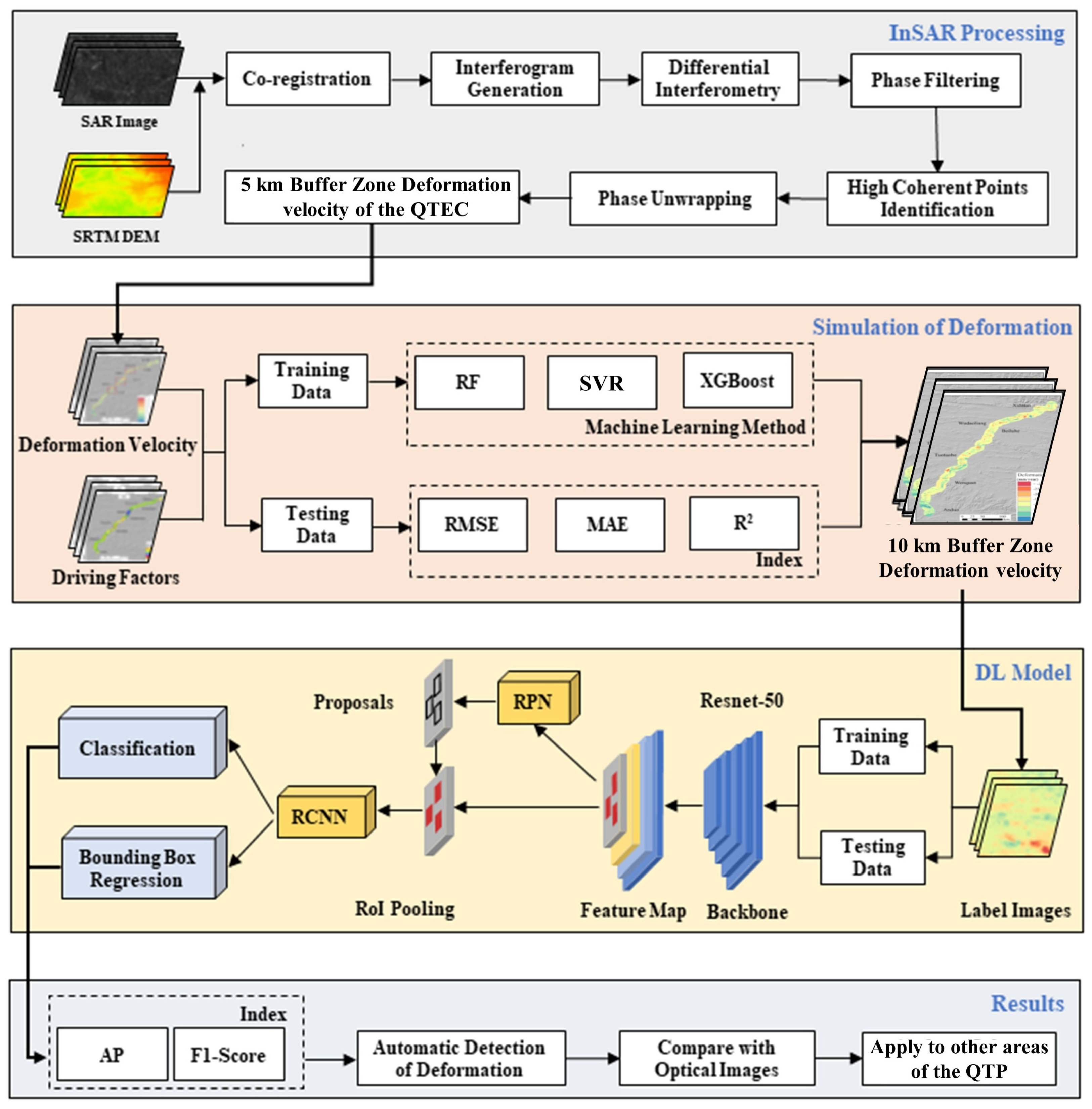
Based on related studies [37,38], nine driving factors of thaw settlement, including three topographic factors (elevation, slope, and orientation), two topographic indices (topographic wetness index (TWI) and NDVI), two permafrost-related factors (volumetric ice content (VIC) and active layer thickness (ALT)), and two climate-related factors (MAGT and annual mean precipitation), were chosen to establish a spatial database.

The elevation data were obtained from the Shuttle Radar Topography Mission (SRTM) digital elevation model (DEM) with a 90 m resolution. This resolution was selected to balance computational efficiency with data accuracy requirements in this study. The slope and orientation data were calculated from the DEM data using ArcMap 10.2 software. The TWI was calculated using ArcGIS 10.2 software packages or manually using the DEM and other spatial data. The NDVI data were calculated using Landsat-8 images with 30 m resolution. The VIC was calculated based on the method proposed by Wu et al. (2004) [39]. The calculation of the VIC is provided in Appendix A. The ALT levels were obtained from a dataset published by Pan et al. (2016) [40]. The MAGT is a critical factor that represents the permafrost thermal status and can be used to distinguish permafrost from seasonally frozen soil [37]. The MAGT data used in this study, at a depth of zero annual amplitude (10–25 m) with 1000 m resolution, were derived from the dataset published by Ran et al. (2021) [36]. The precipitation data were from the 2018 ERA5 meteorological reanalysis data released by the European Center for Medium-Range Weather Forecasts (ECMWF). The spatial resolution of the precipitation was 1000 m. Figure 2 shows the nine driving factors identified. To ensure consistency in resolution, the spatial resolutions of all environmental factors were uniformly resampled at 100 m. Because these data have different values and magnitudes, they were normalized before entering the learning algorithm.

3. Method

In this paper, we used the InSAR and machine learning methods to simulate and detect the permafrost deformation. We first derived surface displacement measurements across the permafrost region using the time-series InSAR method. Then, machine learning models (RF, SVR, and XGBoost) were trained to predict deformation in decorrelated zones using environmental factors. Finally, the completed deformation field served as input to a Faster R-CNN architecture to detect the deformation regions. A technical flowchart is shown in Figure 3.

3.1. Deformation Estimation Using InSAR

The small baseline subset-InSAR (SBAS-InSAR) method [41] is a classical time-series InSAR technique that can be used to obtain ground deformation data over non-urban areas with high accuracy [30]. SBAS-InSAR has been successfully applied to obtain ground deformation in permafrost regions worldwide [42,43,44]. In this study, SAR images were processed using the SBAS-InSAR technique.

First, all SAR images were co-registered with the master images. For Sentinel-1 images, the enhanced spectral diversity (ESD) method was used, with an accuracy of over 1/200 pixels [45]. Interferometric pairs were then generated with a temporal baseline of less than 100 days and a spatial baseline of less than 150 m, and 128 interferometric pairs were identified. In the interferogram-generation process, multi-looking was performed, with 2 looks in the azimuth direction and 8 in the range direction. The Goldstein filter method was used to suppress the noise in the interferometric phase [46]. To further reduce the effect of temporal decorrelation, points with low coherence were masked. In this study, the coherence threshold was set to 0.7. After that, the minimum cost flow (MCF) method was utilized to unwrap the filtered interferometric phase. The deformation parameters of the selected points were estimated with the least-squares method. Subsequently, the residual phase was generated by removing the model phase of the deformation rate and the DEM error from the original interferometric phase. Then, the atmospheric components were estimated using spatial low-pass triangular filtering and temporal high-pass linear filtering and subsequently subtracted. After that, the LOS (line of sight) displacement was converted into the vertical displacement by dividing the cosine of the SAR incidence angle (θ). More details on SBAS-InSAR can be found in Berardino et al. (2002) [41] and Lanari et al. (2004) [47].

To validate the accuracy of the deformation results derived from the Sentinel-1A images, we compared deformations in the overlapping segments of two tracks (track 150–475 and track 77–475).

3.2. Deformation Simulation Using Machine Learning

In this study, we utilized three machine learning algorithms, including random forest (RF), support vector regression (SVR), and XGBoost, along with deformation data and various driving factors of permafrost thawing to simulate ground deformation in permafrost regions [42,48]. RF and SVR are both highly regarded machine learning algorithms that have demonstrated excellent performance in solving high-dimensional feature problems in different fields. XGBoost is an improved version of the gradient boosting decision tree (GBDT) that effectively addresses the overfitting problem in the GBDT. It has exhibited good performance in simulating deformations in arid areas [49].

3.2.1. Random Forest

RF is a method of ensemble learning consisting of numerous decision trees that is frequently utilized in applied statistics [50,51]. This algorithm employs the principle of bagging, where it trains multiple trees using bootstrap samples from the training dataset and aggregates the predictions of these trees through averaging.

A sequence of regression models {$t_1\left(x\right)$, $t_2\left(x\right)$, $t_3\left(x\right)$, …, $t_k\left(x\right)$} was obtained by n-time model training and utilized to construct a multi-regression model system [31]. The formula for the regression decision is as follows:

$${\widehat{f}}_{rf}^K\left(x\right)\sum _{k=1}^K{t}_i\left(x\right)$$

(1)

where ${\widehat{f}}_{rf}^K(x)$ represents the collective regression model, $t_i$ denotes each individual decision tree regression model, and K stands for the quantity of regression trees (N estimators).

Typically, as the number of decision trees increases, the prediction error of the model gradually decreases and stabilizes. After continuous parameter tuning, it was finally determined that the number of decision trees should be set to 100 and the number of leaf nodes to 1.

3.2.2. Support Vector Regression

SVR is an application of SVM (support vector machine) that seeks to identify linear hyperplanes by aligning multidimensional input vectors with the corresponding output values. Subsequently, the acquired model is utilized to forecast forthcoming output values within a designated test dataset [52].

For a set of data points $\mathrm{P}=(x_i,a_i)$, i = 1, …, n, the hyperplane constructed using SVR is determined as follows:

$$f\left(x\right)=a_i{x}_i+b$$

(2)

where $x_i$ represents the input vector for data point i, $a_i$ is the actual value, and n denotes the number of data points. Equation (2) resembles a linear regression model, where the predicted value of f(x) hinges on the slope (a) and intercept (b).

The penalty coefficient in SVR serves to enhance the model’s classification ability [52]. In this study, the penalty factor was set to 40, and the radial basis function parameter was set to 60.

3.2.3. Extreme Gradient Boosting

XGBoost stands out as a sophisticated supervised learning algorithm within the gradient boosting framework [53]. This algorithm employs “gradient boosting” to combine multiple “weak learners” and produce accurate results. XGBoost has achieved remarkable success in various machine learning competitions, earning widespread recognition in the field [54].

In the XGBoost model, the learning rate controls the step size of each update and is an important hyperparameter. A learning rate that is too small may lead to overfitting, while a learning rate that is too large may cause the model to fail to converge. Increasing the number of iterations can generally improve the model’s performance, but it can also lead to overfitting [54]. After continuous parameter tuning, it was finally decided to set the number of iterations to 100 and the learning rate to 0.1.

3.2.4. Training and Testing Samples

Using random sampling, we extracted the same number of points from non-subsidence points as there were subsidence points to form the sample set. In the sample set, 70% of the points were used as the training set for tuning parameters and training the model, while the remaining 30% were used as the test set for calculating the model’s training accuracy. In both the training and test sets, the ratio of subsidence points to non-subsidence points was maintained at 1:1 [55].

The nine driving factors used in this study were VIC, MAGT, DEM, orientation, slope, TWI, NDVI, ALT, and precipitation. To evaluate potential multicollinearity issues in our predictive models, we primarily employed Pearson correlation coefficients and variance inflation factors (VIFs) to assess multicollinearity among predictor variables. After collinearity analysis, all nine driving factors met the requirements, so no factors needed to be excluded. The nine driving factors were used as independent variables, and the deformation values were used as dependent variables. The influencing factors were input as training samples, and the output result was the potential deformation value for each sample.

3.3. Deformation Automatic Detection Using DL

After obtaining the simulated deformation maps, a deep learning model was employed to identify the regions experiencing deformation. The objective of this approach was to automate the detection of deformation regions related to permafrost thawing.

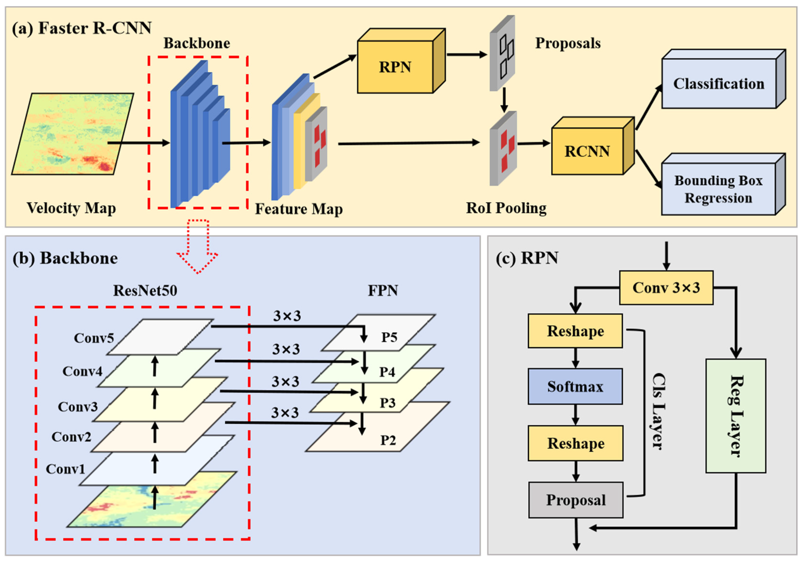
3.3.1. Automatic Detection Model

The deep learning model utilized in this study was the Faster R-CNN model, which offers the main advantage of enhanced detection speed without compromising accuracy [25]. This model operates through four logical stages, ensuring efficient and precise object detection, as shown in Figure 4a. First, the input image is transformed into a multidimensional array, typically referred to as a tensor with dimensions of (height, width, depth). This tensor is then fed into a pre-trained CNN model to generate a convolutional feature map [56]. In this study, ResNet50 and a feature pyramid network (FPN) were used as feature extractors, as shown in Figure 4b. The extracted feature maps are then input into the next section. This method finds frequent application in transfer learning, especially when leveraging network weights trained on extensive datasets to train classifiers for smaller datasets.

Subsequently, the feature map passes through a network called a region proposal network (RPN), which detects potential object-containing regions. Classical detection methods use sliding windows or selective search methods to produce detection frames, which can be computationally intensive [56]. In contrast, Faster R-CNN streamlines this process by directly utilizing the RPN to generate detection frames. This represents a significant benefit of Faster R-CNN, as it substantially enhances the efficiency of detection frame generation [56], as shown in Figure 4c. Following the RPN, frames that may contain objects are obtained. By combining these frames with the feature maps extracted from the original image in the first part, the corresponding objects can be identified, and their features can be extracted into new tensors for classification using the Region of Interest (RoI). Finally, the objects are classified by the R-CNN module, which uses the information obtained in the previous section to adjust the bounding box and make it more accurate. Specifically, after obtaining the proposal feature maps from RoI pooling, the proposals are classified by fully connected layers and Softmax, and bounding box regression is performed on the proposals to obtain a higher-precision box [56].

To evaluate the detection performance of the Faster R-CNN model in this study, we selected three common deep learning object detection methods: SSD [57], YOLOv5 [58], and RetinaNet [59]. These models are all single-stage detectors, which offer faster inference speeds while maintaining reasonably high accuracy.

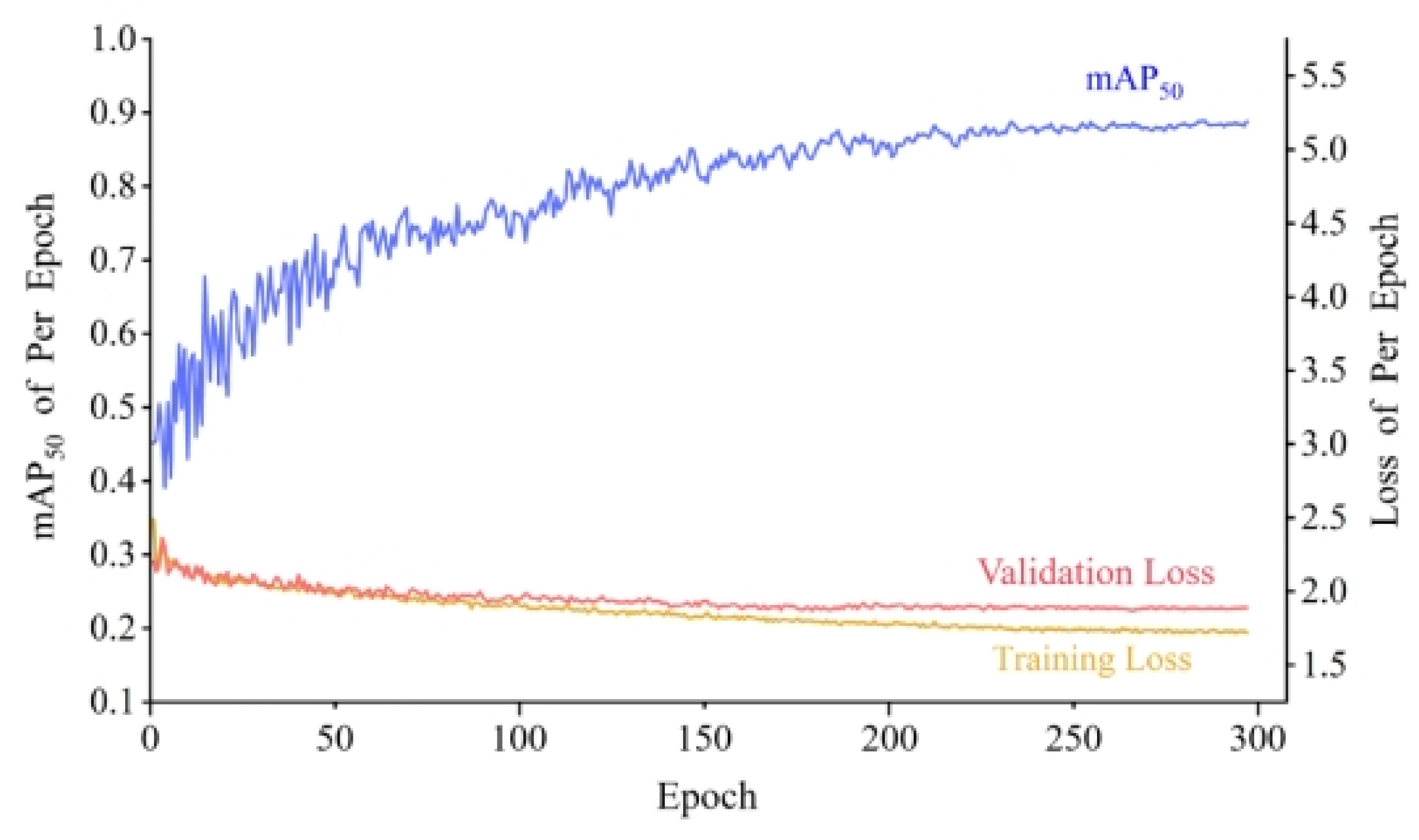
3.3.2. Training Settings and Accuracy Verification

Training samples are important for deep learning. According to expert knowledge and the relevant literature [10,53,54,55,56,57,58,59,60], and confirmed through repeated experiments, we set a deformation threshold of −16 mm/year on the deformation rate map of the 10 km buffer zone and then divided it into sub-regions of equal length and width. Variations in the lengths of the distinct regions were introduced to enrich the features of the deformation areas within the samples. After the samples were annotated using the LabelImg tool, they were divided into training and testing sets at a ratio of 0.85:0.15. Some of the training and predicted samples are shown in Figure 5a–c and Figure 5d–f, respectively.

Four indicators were used to evaluate the accuracy of the deep learning model: average precision (AP), recall, precision, and F1-score. AP is a comprehensive measure of a model’s performance in a task that considers the accuracy under different recall values and averages them on a weighted basis. The calculation formula for AP is as follows:

$$\mathrm{A}\mathrm{P}=\left({\displaystyle \frac{1}{\mathrm{n}}}{\mathsf{\Sigma }}_{\left(\mathrm{r}\in {\displaystyle \frac{1}{\mathrm{n}}},{\displaystyle \frac{2}{\mathrm{n}}}\dots {\displaystyle \frac{\mathrm{n}-1}{\mathrm{n}}},1\right)}{\mathrm{P}}_{\left(\mathrm{r}\right)}\right)$$

(3)

where n represents the number of detection points and ${\mathrm{P}}_{\left(\mathrm{r}\right)}$ represents the accuracy value when the recall is r. In addition, recall, precision, and the F1-score were used as auxiliary evaluation indices. Their formulas are as follows:

$$\mathrm{R}\mathrm{e}\mathrm{c}\mathrm{a}\mathrm{l}\mathrm{l}={\displaystyle \frac{\mathrm{T}\mathrm{P}}{\mathrm{T}\mathrm{P}+\mathrm{F}\mathrm{N}}}$$

(4)

$$\mathrm{P}\mathrm{r}\mathrm{e}\mathrm{c}\mathrm{i}\mathrm{s}\mathrm{i}\mathrm{o}\mathrm{n}={\displaystyle \frac{\mathrm{T}\mathrm{P}}{\mathrm{T}\mathrm{P}+\mathrm{F}\mathrm{P}}}$$

(5)

$$\mathrm{F}1={\displaystyle \frac{2\ast \mathrm{P}\mathrm{r}\mathrm{e}\mathrm{c}\mathrm{i}\mathrm{s}\mathrm{i}\mathrm{o}\mathrm{n}\ast \mathrm{R}\mathrm{e}\mathrm{c}\mathrm{a}\mathrm{l}\mathrm{l}}{\mathrm{P}\mathrm{r}\mathrm{e}\mathrm{c}\mathrm{i}\mathrm{s}\mathrm{i}\mathrm{o}\mathrm{n}+\mathrm{R}\mathrm{e}\mathrm{c}\mathrm{a}\mathrm{l}\mathrm{l}}}$$

(6)

where TP denotes true positive, FP denotes false positive, and FN denotes false negative. Furthermore, a comparative analysis of PR curves was conducted across different models.

The network parameters were updated and optimized using the Adam optimizer. The number of iterations, learning rate, and batch size were set to 300 epochs, 1 × 10⁻³, and 9, respectively.

4. Experimental Results

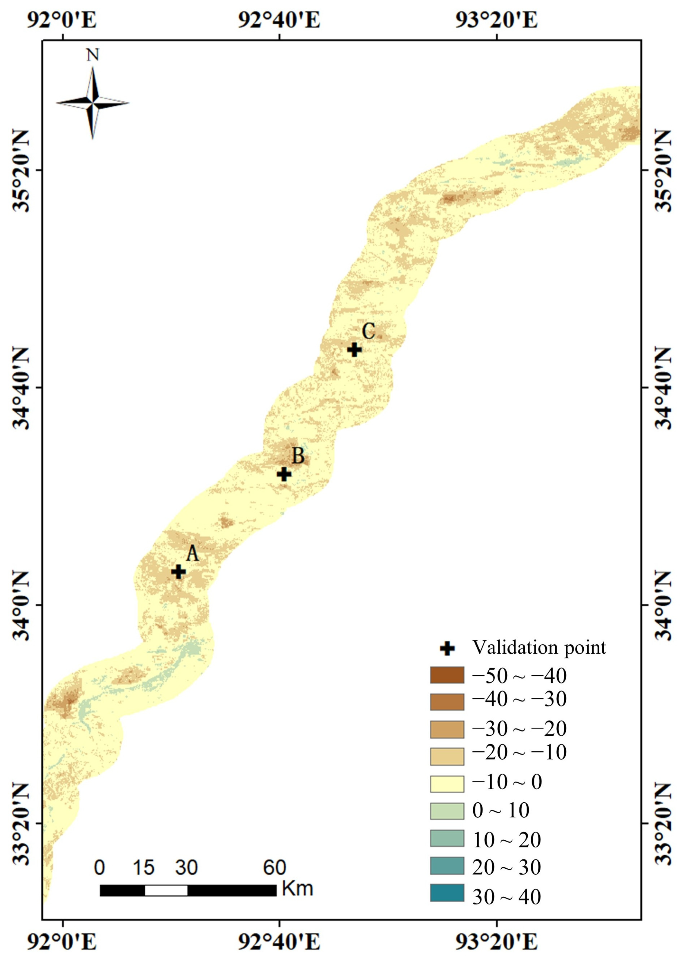
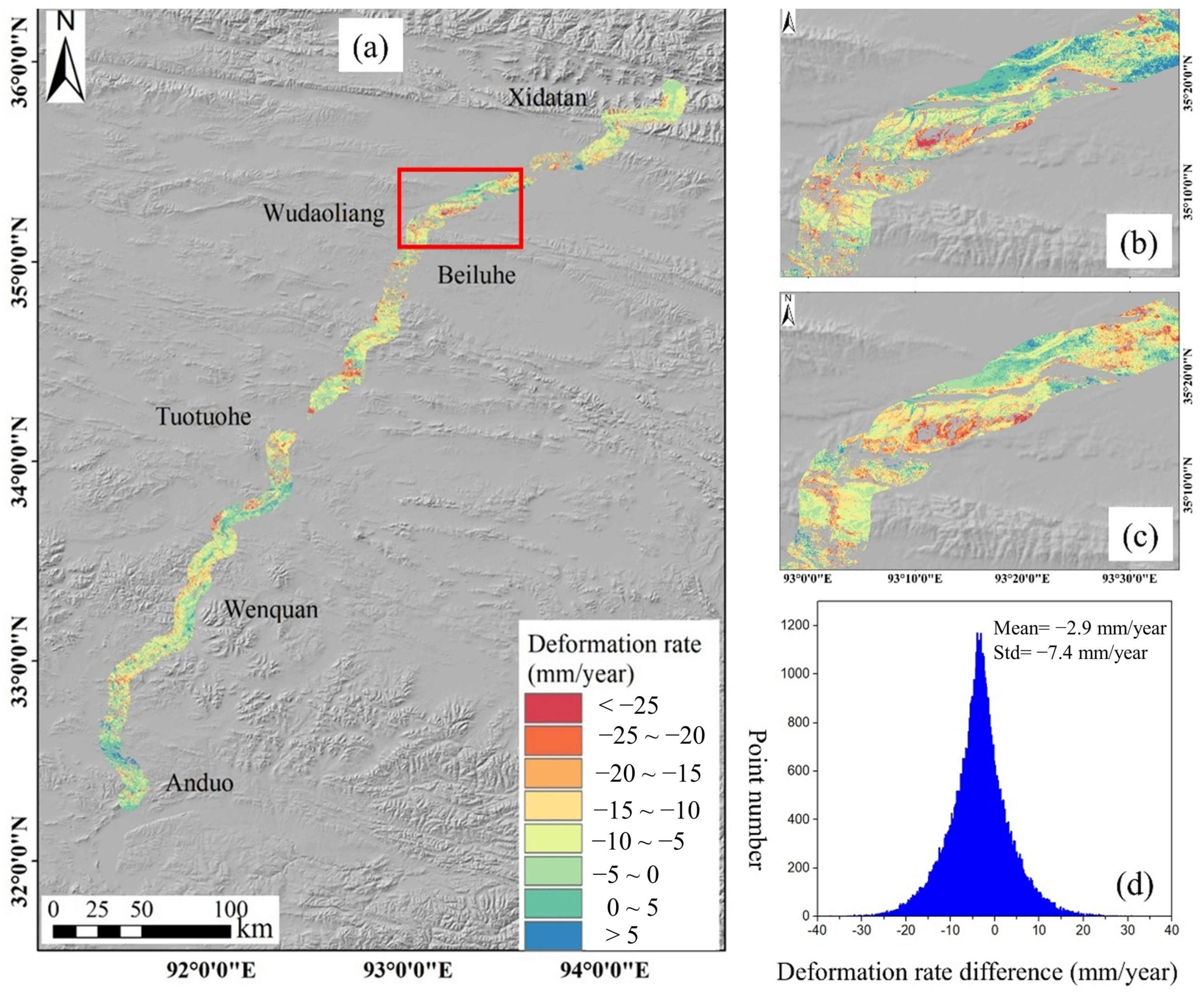
4.1. InSAR Results

The ground deformation along the QTEC from 2017 to 2018, using Sentinel-1A images, is shown in Figure 6a. The distribution of the deformation rate varied widely throughout the study area, and the average annual surface deformation rate of the whole study area was −7 mm/year. In some local areas, our deformation data show that the deformation rate was up to −60 mm/year in the most heavily subsided areas and up to 42 mm/year in the most significantly uplifted areas. Obvious subsidence deformation rates were detected in some areas, such as Tuotuohe, Fenghuoshan, Beiluhe, Wudaoliang, and Chumaerhe, which is consistent with the findings of earlier research [10,61,62]. We compared the ground deformation of the Beiluhe section with the results of other researchers; most previous studies indicated that this region shows obvious deformation with velocity ranges from 0 to −20 mm/year. The serious ground subsidence in those regions may be due to the high MAGT, intensive human activities, and the high ice content of the ground ice. Given the limited spatial and temporal scope of our observations, geological factors are not the primary drivers of surface deformation.

We analyzed the deformation differences among points within these overlapping areas, as shown in Figure 6b,c. Consistent results were observed in the overlapping sections. The overall deformation trends between the two tracks were generally consistent. Figure 6d illustrates the statistical distribution of these differences, showing a mean value of −2.9 mm/year and a standard deviation (STD) of 7.4 mm/year. In addition, we compared the InSAR results with the leveling results from other research [63]. Three leveling points (the A, B, and C locations in Figure A1) during the observation period from 4 January 2018 to 9 February 2018 were used for validation. The errors between the leveling results and the InSAR results at the three points were 1.7, 4.9, and 5.4 mm, confirming the validity of the InSAR results.

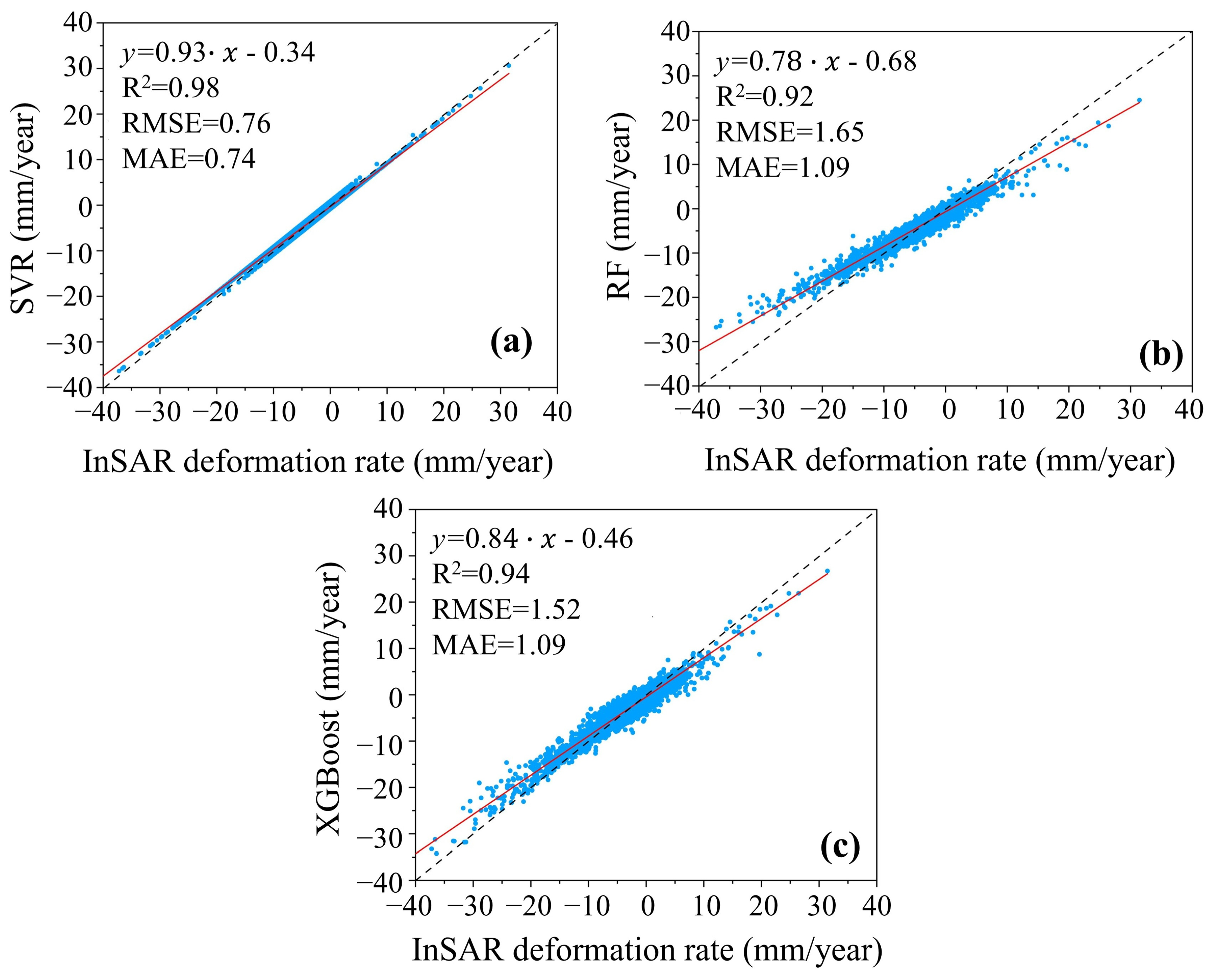
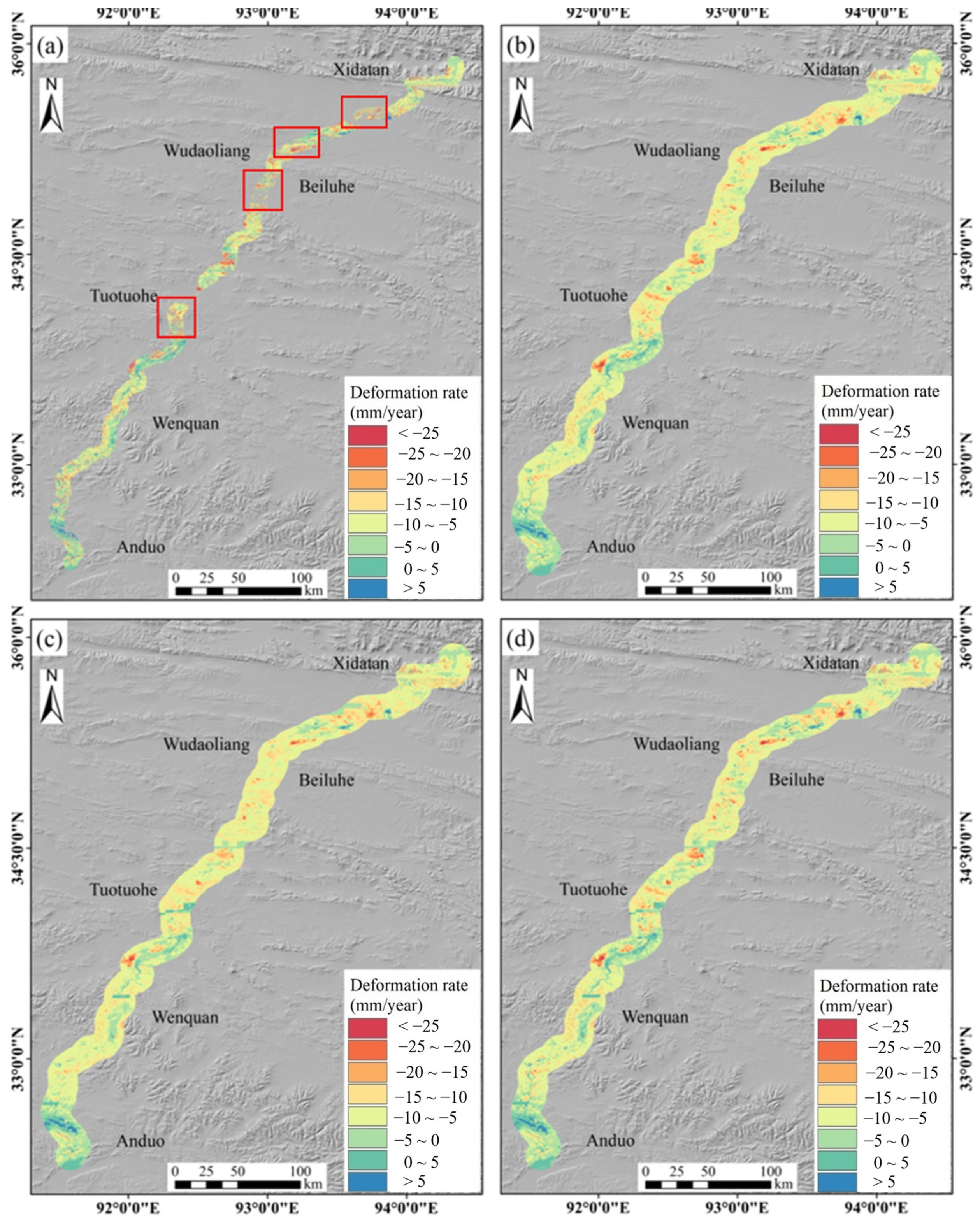
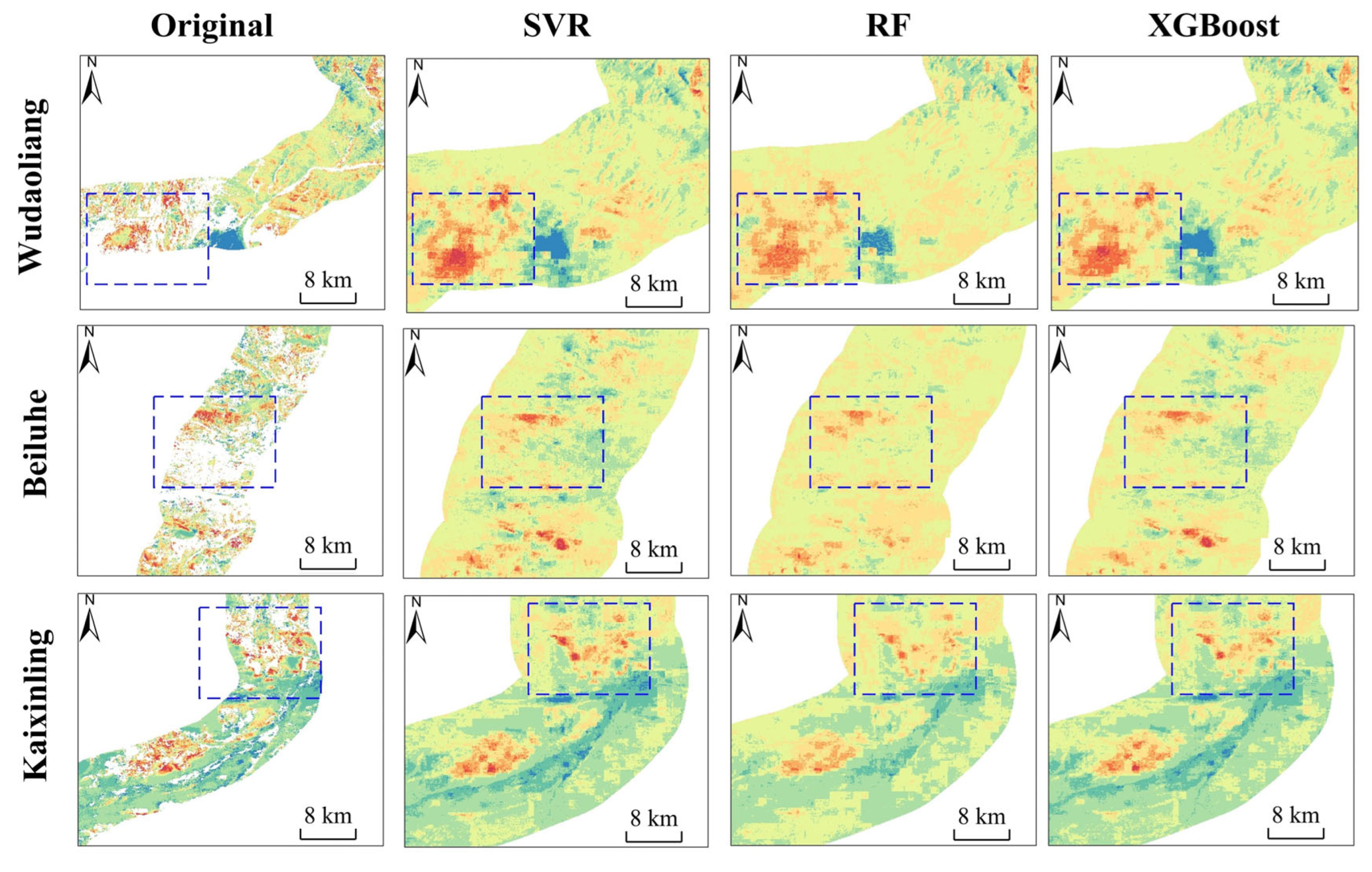
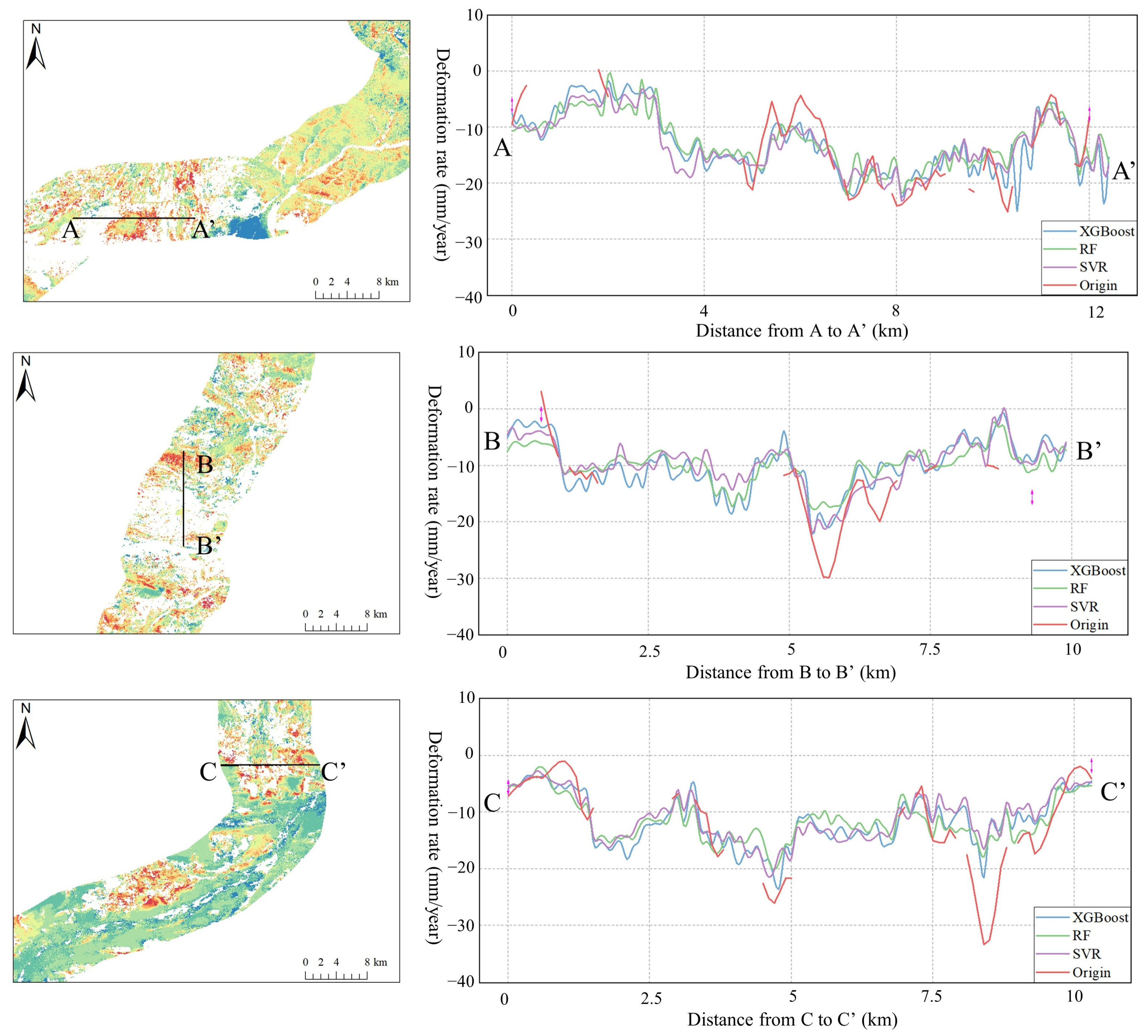
4.2. Performance of the Three Machine Learning Models

Scatter plots of the deformation results and testing phase of the applied algorithms are shown in Figure 7, indicating a correlation between the deformation rate calculated using the applied algorithms and the permafrost InSAR data. The figure demonstrates that the SVR trend line was closer to the dashed black line than that of the other two models, as shown in Figure 7a–c. We can see that the best-performing algorithm was SVR, with R2, RMSE, and MAE values of 0.98, 0.76 mm/year, and 0.76 mm/year, respectively. The correlation between the data prediction results and deformation data was good, and the scatter plots of SVR against the InSAR data were more condensed than those of XGBoost and RF.

Although SVR appears to be superior to the other methods in terms of various indicators for this research area, the XGBoost method can better prevent the overfitting of the training dataset and generalize the model well, particularly when handling large datasets. XGBoost does not consider variable preprocessing and missing values; instead, it relies on the normal distribution of data, making it more time-consuming than other more complex machine learning methods.

The predicted deformation rate results obtained using the various algorithms in the 10 km buffer of the QTEC are shown in Figure 8. The surface velocity simulated using the machine learning methods resolves some gaps. The frequency histogram indicates that the mean values of the obtained deformation results were different. The µ values corresponding to the SVR, RF, and XGBoost methods were −7.06, −7.60, and −7.20 mm/year, respectively.

According to the deformation rate, the subsidence velocity was divided into six categories: −5 to 0; −10 to −5; −15 to −10; −20 to −15; −25 to −20; and <−25 mm/year (

Table 1. The percentage of deformation rate generated using algorithms for different subsidence levels.

Deformation Rate (mm/year)	−5~0	−10~−5	−15~−10	−20~−15	−25~−20	<−25
SVR	0.3	1.0	3.8	18.2	53.4	23.3
RF	0.2	0.7	3.5	21.4	55.8	18.5
XGBoost	0.4	1.10	4.1	17.8	51.6	24.9

). Overall, the results of all the models were concentrated in the lower region, which is the region with a deformation rate of −10 to −5 mm/year, and the differences between several models were mainly concentrated at −10 to −5 and −5 to 0 mm/year. The SVR algorithm with the highest regression accuracy predicted approximately 1.3% of the areas as larger settlement areas with subsidence rates larger than 20 mm/year, and approximately 76.7% of the areas were classified as stable and lower areas.

To compare the differences among the three methods, three regions (Wudaoliang, Beiluhe, and Kaixinling) with significant settlement deformation rates and blank areas are illustrated in Figure 9. The dashed and blue boxes in the figure represent the typical parts of the selected areas. In the Wudaoliang and Kaixinling areas, all three methods predicted significant settlement in the blue-boxed area; however, compared with the original deformation rate, the accuracy of the RF method was lower than that of the other two methods. In the Beiluhe region, the RF method was also significantly weaker than the other two methods in predicting uplift areas.

Figure 10 shows a comparison between the deformation rates obtained using InSAR and those simulated using the three machine learning methods for complementation. Profiles AA’ and CC’ span more than 10 km and extend from west to east, while profile BB’ extends 10 km from point B to point B and covers a route from north to south. We can observe that the deformation profile lines generated using the three simulation methods closely align with the results from InSAR, demonstrating good agreement. They also provide effective approximations for areas with missing deformation data. Overall, the SVR method performed best, and the deformation rates obtained from the simulation of this method had the smallest difference from those obtained from InSAR. It is important to note that there were slight differences between the deformation estimated from the machine learning method and the InSAR results, particularly in areas without deformation, where significant high-frequency signals were observed. It is inferred that these high-frequency signals may be due to inconsistencies in the original spatial resolution of different factors. Additionally, the machine learning estimates tended to underestimate deformation compared to the original InSAR deformation, especially in areas with extreme deformation values. However, overall, the deformation estimates based on the machine learning method showed good consistency with the original deformation data.

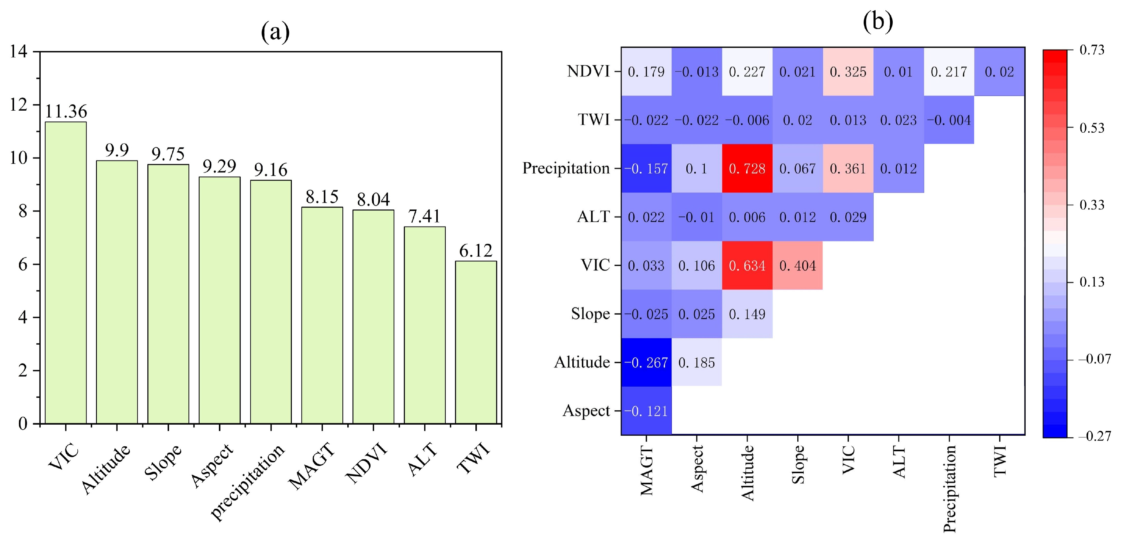
4.3. Correlation and Importance Analysis of Various Factors

To assess the importance of each factor, the RF algorithm systematically switches one input feature while holding the others constant and measures the resulting decrease in accuracy using out-of-bag (OOB) error estimation [51]. As shown in Figure 11a, the resulting importance rankings, from highest to lowest, were VIC, altitude, slope, aspect, precipitation, MAGT, NDVI, altitude, and TWI. The primary cause of permafrost thaw deformation is the melting of ground ice, which has a direct relationship with the VIC. In this study, the VIC achieved the highest ranking, which is consistent with the findings of numerous previous studies [37,38]. After the VIC, altitude was the most influential factor contributing to deformation in the QTEC.

The correlation analysis among the different factors is presented in Figure 11b. Some environmental factors indicated an obvious relationship. The strongest positive correlation was observed between precipitation and altitude, with a correlation coefficient of 0.72. The second highest positive correlation was found between the VIC and slope, with a correlation coefficient of 0.63. Among the negative correlations, the MAGT was negatively correlated with altitude (correlation coefficient of −0.26), followed by the correlation between the MAGT and precipitation (correlation coefficient of −0.15). The ALT and TWI showed relatively weak correlations with other factors.

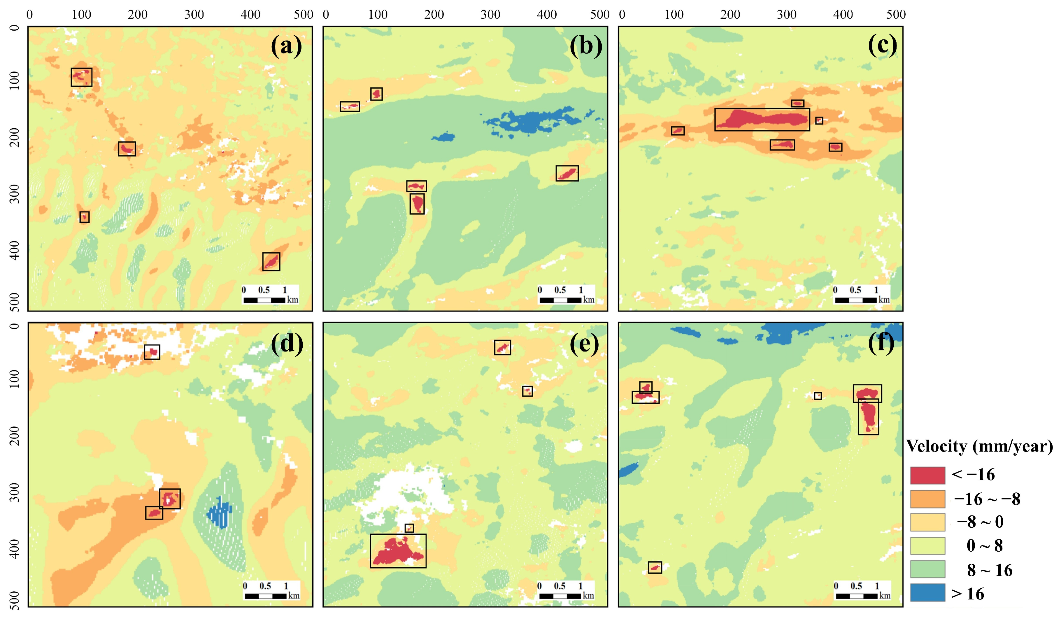
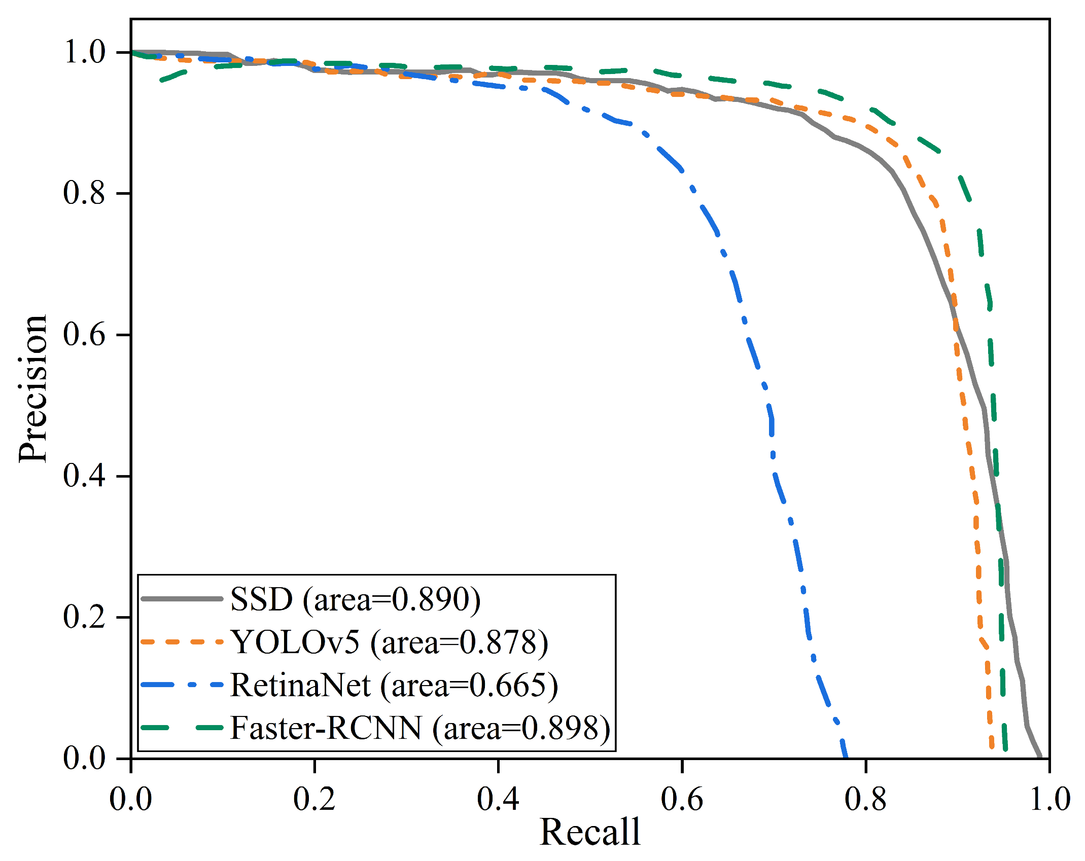
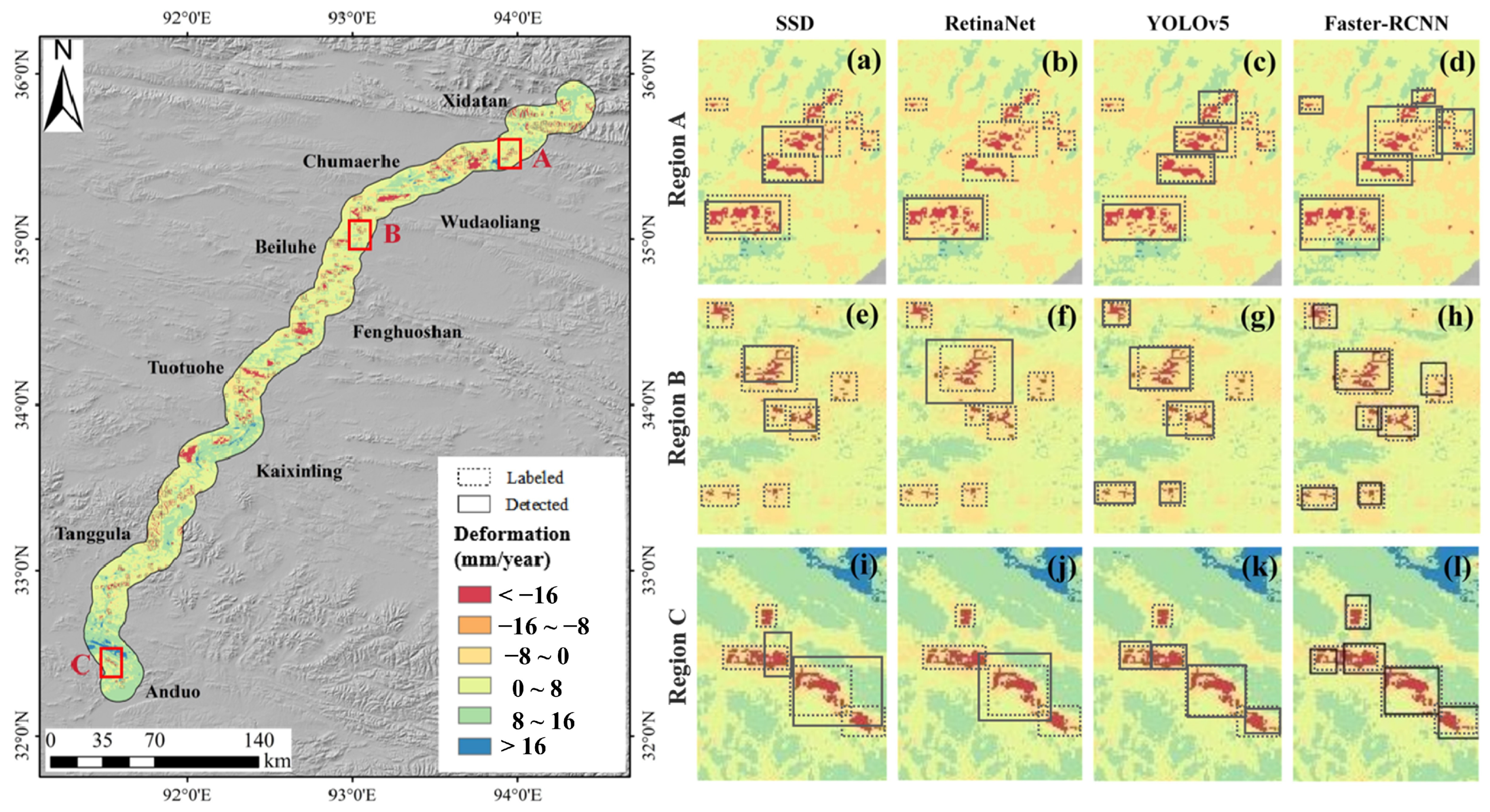
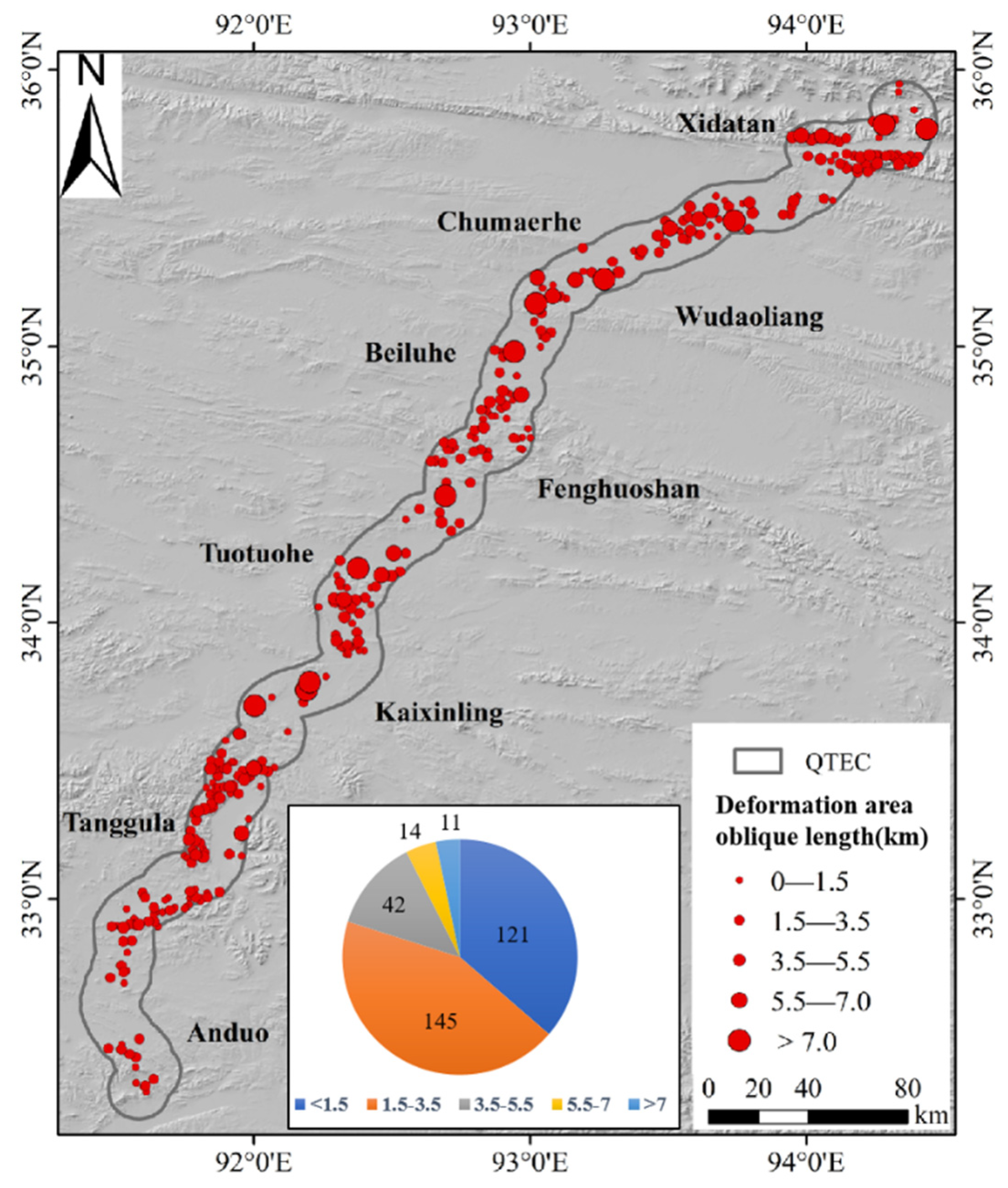
4.4. Detection of Permafrost Deformation Regions

The Faster R-CNN model was fully trained on the training set. Figure 12 shows the decrease in training loss and validation loss as well as the change in model accuracy over epochs during training. In the initial stage, the loss values dropped sharply, indicating a reasonable learning rate and effective gradient descent. As training progressed, the loss curves gradually stabilized and eventually converged. After the training process, the AP and F1-score metrics were calculated to assess the performance of the Faster R-CNN model during deformation region detection on the test set. We established two AP metrics with different intersection over union (IoU) thresholds, i.e., AP50 and AP50-95, to evaluate model performance under various IoU conditions. Based on the calculations, the Faster R-CNN model achieved AP50 and AP50-95 scores of 0.898 and 0.540, respectively, on the test set, with an associated F1-score of 0.850. Overall, the AP of the model reached high levels across most IoU conditions.

To further validate the superiority of the Faster R-CNN model over other deep learning approaches, we trained three additional models, including SSD, YOLOv5, and RetinaNet, and assessed their accuracy on the test set, as shown in

Table 2. Detection accuracy of the four models.

Method	Backbone	F1-Score	AP50 (%)	AP50-95 (%)
SSD	VGG	0.82	87.8	51.4
YOLOv5	CSPDarknet	0.82	89.0	53.2
RetinaNet	ResNet50	0.66	66.5	41.2
Faster R-CNN	ResNet50	0.85	89.8	54.0

. Taking the AP50 metric as an example, Figure 13 presents a comparison of precision between the Faster R-CNN model and three comparative models. The results indicate that the detection accuracy of the Faster R-CNN model surpassed that of the other three models, demonstrating its robust training performance for automated detection tasks of deformation regions on deformation maps.

Permafrost thawing is widespread in the QTP, resulting in serious ground deformation, particularly in some sections of the QTEC [5]. To detect permafrost thawing-related deformation accurately and quickly, we utilized the trained SSD, RetinaNet, YOLOv5, and Faster R-CNN models to detect deformation from the simulated deformation data of a 10 km buffer zone in the QTEC. The detection results are presented in Figure 14, which indicates that the detection effect of the Faster R-CNN model was remarkable and significantly better than that of the other three comparative models. The deformation rate map gives special attention to areas where the subsidence rate was greater than a certain threshold. We determined this threshold to be 16 mm/year through multiple tests in this study. At the same time, the deformation regions detected using the Faster R-CNN model are clearly labeled, and these regions are marked with black boxes. Through a detailed analysis, we found that the Faster R-CNN model could accurately detect the deformation regions in most cases. Although some small deformation areas may have been missed in rare cases, the deformation detection accuracy of this model was generally high. This provides powerful data support for the further study of permafrost thaw slumping and helps to understand the environmental factors contributing to the formation of thermal thaw slumps.

5. Discussion

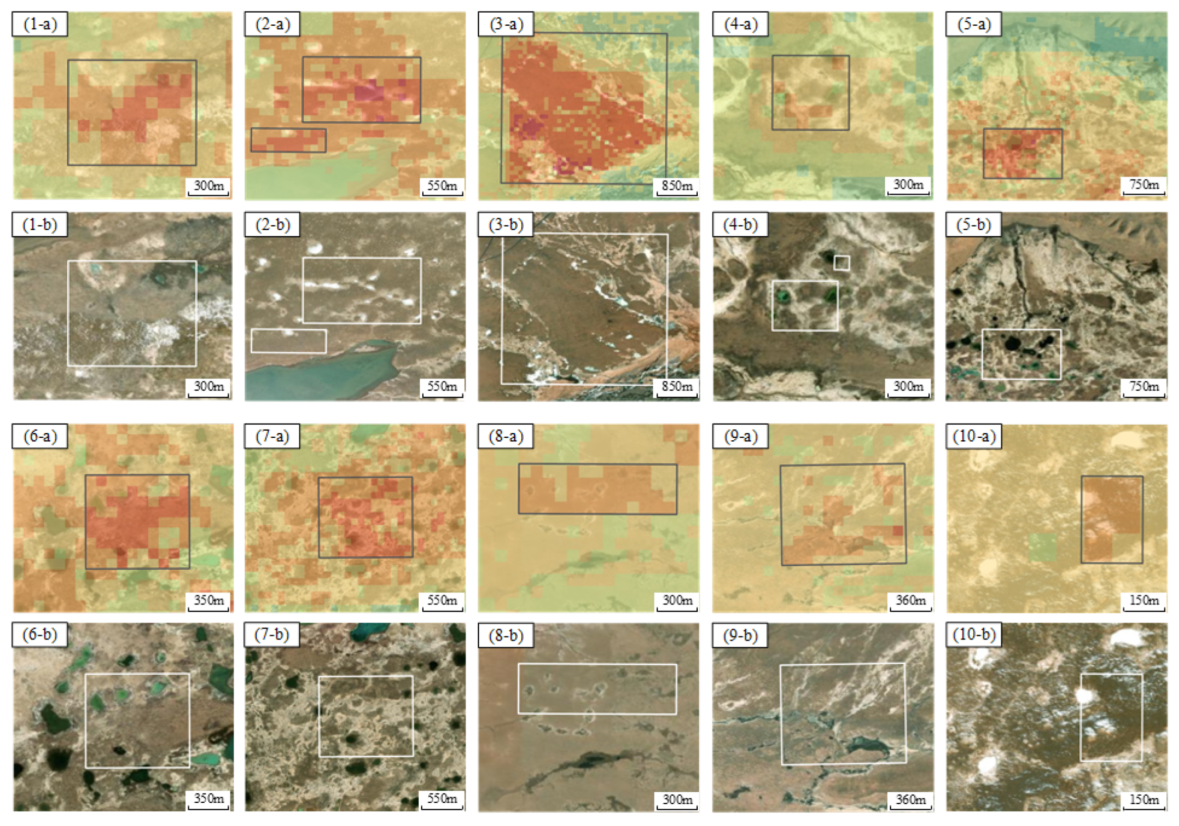
5.1. Detection of Obvious Settlement Regions Along the QTEC

Using the proposed R-CNN model, we detected over 300 settlement areas within the 10 km buffer zone along the QTEC, as shown in Figure 15. Based on the size of the detection boxes, we roughly estimated the area of detected regions, with most settlement areas having a slope length of less than 3.5 km. After detecting the deformation areas with Faster R-CNN, we superimposed the detection results on the optical images for comparison. In the regions where the subsidence rate exceeded 16 mm/year, subsurface ice melting induced the development of a series of thermal thaw phenomena, which mainly manifested as thermokarst lakes, thermal thaw subsidence in flat regions, and RTSs in slope regions, all of which showed distinct characteristics in the optical images.

Figure 16 shows 10 cases of thermokarst lakes and detected deformation areas. Cases 1–7 represent the 5 km real deformation data and their optical images, while cases 8–10 correspond to the 5–10 km region in the 10 km simulated deformation data, along with the corresponding optical images. Specifically, in the case illustrated in Figure 16, the deformation area is dotted with numerous thermokarst lakes that may expand and join to form larger lakes or ponds as time passes, and the permafrost will continue to thaw.

We collected the published inventoried RTS data from Xia et al. (2022) [20] and thermokarst lake data from Mu et al. (2023) [64] and compared the collected data with the detected deformation areas using the Faster R-CNN model, as shown in Figure 17. From the publicly released data, we observed that the RTSs and thermokarst lakes are primarily distributed in the vast permafrost area between the Chumar River and the Tuotuo River. However, there are not many cataloged RTSs within the QTEC. Nevertheless, we identified several cataloged RTSs that are consistent with the deformation areas we detected, as shown in the subfigure in Figure 1. We found that the deformation areas we detected do not completely align with the publicly released RTSs, which may be due to the following two reasons. On one hand, permafrost degradation does not necessarily lead to RTSs, but it will certainly cause ground subsidence. The formation of RTSs is influenced by topography and soil moisture content. On the other hand, the existing RTS data were detected using high-resolution optical images based on the texture features, which capture the phenomenon in a stable state. For those RTSs that are in their early developmental stage, there may not be significant textural changes on the ground, making them undetectable in optical images. However, these early-stage instances of thermal thawing and collapses can still result in significant surface deformation, which can be detected by InSAR. This indicates that the InSAR-based deformation results can help to detect potential RTSs or early-stage RTSs. In addition, thermokarst lakes are distributed in some of the detected deformation areas, which further indicates that the InSAR results are helpful for monitoring the degradation of permafrost.

Compared to other studies utilizing deep learning for deformation recognition, such as those of Wu et al. (2023) [26], who employed Oriented R-CNN models to automatically detect ground subsidence in delta metropolitan areas, and Cai et al. (2023) [25], who used improved Faster R-CNN models to automatically detect landslides in Guizhou Province, our study employed machine learning methods to simulate and address gaps in InSAR results. This approach yields more deformation information than pure InSAR methods, facilitating more comprehensive deformation recognition. Xia et al. (2022) [20] utilized the DeepLabv3+ model to automatically identify RTSs in permafrost regions along the QTEC using high-resolution optical images. Compared to Xia’s work, our study employed the InSAR method, which is more effective in detecting potential permafrost degradation areas than optical images.

In summary, our results clearly show that deformation data simulated by machine learning are available. The performance of the Faster R-CNN model was particularly excellent when used for deformation detection. These findings strongly support future research. Notably, in the permafrost regions of the Qinghai–Tibet Plateau, geological activities (e.g., tectonic movements) can induce surface deformation that may confound monitoring signals of permafrost degradation. While our current study did not explicitly account for these geodynamic influences, we argue their impact is limited for two reasons: (1) the QTEC has a limited spatial extent of only 10 km in width and (2) the short observation period minimizes cumulative tectonic effects. Future large-scale automated detection of permafrost deformation should incorporate geological activity corrections.

5.2. Generalization Ability of Deep Learning Models

To test the generalization ability of the model and ensure its effectiveness in detecting other regions, we targeted other regions of the QTP for deformation detection using our well-trained Faster R-CNN model.

The Zonag Lake–Yanhu Lake Basin is a representative region located at 90°30′E to 93°45′E and 35°20′N to 35°55′N. We collected deformation data of the basin from 2017 to 2020 (Figure 18a) and used the Faster R-CNN model to detect the deformation areas, as shown in Figure 18b. As the detection outcomes of the model were represented by rectangular bounding boxes, we utilized the diagonal length of these bounding boxes as the diameter of the circles. In Figure 18b, the circles of varying sizes approximate deformation regions of different sizes. A total of 956 deformation areas were detected by the model, which were mainly distributed in the eastern part of Kusai Lake, the western part of Zonag Lake, and the hillside along the periphery of the watershed. The size of the deformation areas was categorized into five classes, and the range of the deformation diameters was mainly concentrated from 0.5 to 1.5 km, while the areas with a deformation radius greater than 1.5 km were mainly located in the eastern and northern parts of Kusai Lake.

Four typical areas were selected for analysis at different locations in the basin; their locations, deformation results, and corresponding optical images are shown in Figure 18c–j. The subsidence rate of the four areas was greater than 10 mm/year, indicating that these areas were undergoing obvious permafrost thawing. The optical images show that the vegetation in these areas was sparser than the surrounding features, and the color and texture features were in sharp contrast to the surrounding features, especially in the second area (d and h), where there were clear retrogressive thaw slumps.

After a detailed analysis, we found that the Faster R-CNN model trained using the deformation data from the QTEC region demonstrated excellent generalization ability. This means that the model not only performed well in the region where the training data were located but also automatically detected deformation in other areas of the QTP.

5.3. Limitations

A machine learning-based method was proposed to simulate and detect the permafrost deformation. Our model was trained and tested in the permafrost engineering corridor of the QTP, confirming the effectiveness of the algorithm. In addition, the proposed method was applied to the Zonag Lake Basin to validate its robustness. However, this study had the following limitations:

(1)

For areas with significant incoherence, we relied on machine learning-based deformation simulation results for deformation area detection. Despite the relatively high accuracy of machine learning simulations, some errors in the simulations may lead to bias in the subsequent extraction results. In areas where the deformation values are close to the detection threshold, the underestimation of the results based on machine learning may lead to inaccuracies in the detection outcomes. In regions characterized by high coherence values, employing direct deep learning monitoring rather than machine learning simulations can mitigate errors induced by simulation processes.

(2)

During subsidence area detection, this study only considered deformation information and neglected environmental factors, such as geological conditions, water storage, and vegetation cover, which are crucial for deformation area monitoring [65,66]. In future work, we will integrate deformation and other environmental factors for permafrost thawing region detection.

(3)

Since there are no InSAR results available for other permafrost regions, the proposed method has only been applied in the Zonag Lake Basin. Future testing in other plateau regions will be necessary to validate the effectiveness of the method. This may require a more extensive set of training samples to accommodate the varied demands of different scenarios.

6. Conclusions

In this study, nine driving factors of the surface settlement and deformation at 5 km along the QTEC buffer zone were identified. Three machine learning methods, including RF, SVR, and XGBoost, were used to simulate the deformation data for 10 km along the QTEC. Among them, the SVR algorithm had the best performance (R2 = 0.98, RMSE = 0.76 mm/year, and MAE = 0.74 mm/year). Additionally, the contribution of various factors to the occurrence of land subsidence was evaluated, and the relationship between them was studied. Through FR analysis, it was found that the surface settlement of permafrost along the QTEC was closely related to the VIC, altitude, slope, and ALT. Furthermore, to automatically detect the deformation region of the QTEC, a Faster R-CNN model based on deep learning methods was introduced and applied to other regions of the QTP. The results demonstrate that the model has excellent detection accuracy (F1-score = 0.850, AP50 = 0.898, and AP50-95 = 0.540) and generalization ability.

References

1. Hjort, J.; Streletskiy, D.; Doré, G.; Wu, Q.; Bjella, K.; Luoto, M. Impacts of permafrost degradation on infrastructure. Nat. Rev. Earth Environ. 2022, 3, 24–38. [Google Scholar] [CrossRef]
2. Ran, Y.; Cheng, G.; Dong, Y.; Hjort, J.; Lovecraft, A.L.; Kang, S.; Li, X. Permafrost degradation increases risk and large future costs of infrastructure on the Third Pole. Commun. Earth Environ. 2022, 3, 238. [Google Scholar] [CrossRef]
3. Hjort, J.; Karjalainen, O.; Aalto, J.; Westermann, S.; Romanovsky, V.E.; Nelson, F.E.; Etzelmüller, B.; Luoto, M. Degrading permafrost puts Arctic infrastructure at risk by mid-century. Nat. Commun. 2018, 9, 5147. [Google Scholar] [CrossRef]
4. Chen, F.; Lin, H.; Li, Z.; Chen, Q.; Zhou, J. Interaction between permafrost and infrastructure along the Qinghai–Tibet Railway detected via jointly analysis of C-and L-band small baseline SAR interferometry. Remote Sens. Environ. 2012, 123, 532–540. [Google Scholar] [CrossRef]
5. Wu, Q.B.; Cheng, G.D.; Ma, W.; Niu, F.; Sun, Z.Z. Technical approaches on permafrost thermal stability for Qinghai–Tibet Railway. Geomech. Geoengin. Int. J. 2006, 1, 119–127. [Google Scholar] [CrossRef]
6. Liu, L.; Zhang, T.; Wahr, J. InSAR measurements of surface deformation over permafrost on the North Slope of Alaska. J. Geophys. Res. Earth Surf. 2010, 115, F0302. [Google Scholar] [CrossRef]
7. Du, Y.; Feng, G.; Peng, X.; Li, Z. Subsidence evolution of the Leizhou Peninsula, China, Based on InSAR observation from 1992 to 2010. Appl. Sci. 2017, 7, 466. [Google Scholar] [CrossRef]
8. Shi, X.; Wang, J.; Jiang, M.; Zhang, S.; Wu, Y.; Zhong, Y. Extreme rainfall-related accelerations in landslides in Danba County, Sichuan Province, as detected by InSAR. Int. J. Appl. Earth Obs. Geoinf. 2022, 115, 103109. [Google Scholar] [CrossRef]
9. Rykhus, R.P.; Lu, Z. InSAR detects possible thaw settlement in the Alaskan Arctic Coastal Plain. Can. J. Remote Sens. 2008, 34, 100–112. [Google Scholar] [CrossRef]
10. Feng, X.; Zhang, Z.; Chen, Q.; Guo, Z.; Zhang, H.; Wang, M.; Gao, W.; Liu, X. Integrating remote sensing, GIS, and multi-criteria decision making for assessing PV potential in mountainous regions. Renew. Energy 2025, 241, 122340. [Google Scholar] [CrossRef]
11. Zhang, Z.; Lin, H.; Wang, M.; Liu, X.; Chen, Q.; Wang, C.; Zhang, H. A review of satellite synthetic aperture radar interferometry applications in permafrost regions: Current status, challenges, and trends. IEEE Geosci. Remote Sens. Mag. 2022, 10, 93–114. [Google Scholar] [CrossRef]
12. Ahmed, R.; Siqueira, P.; Hensley, S.; Chapman, B.; Bergen, K. A survey of temporal decorrelation from spaceborne L-Band repeat-pass InSAR. Remote Sens. Environ. 2011, 115, 2887–2896. [Google Scholar] [CrossRef]
13. Duan, M.; Xu, B.; Li, Z.; Wu, W.; Cao, Y.; Liu, J.; Wang, G.; Hou, J. A new weighting method by considering the physical characteristics of atmospheric turbulence and decorrelation noise in SBAS-InSAR. Remote Sens. 2020, 12, 2557. [Google Scholar] [CrossRef]
14. Chen, C.W. A spectral model for multilook InSAR phase noise due to geometric decorrelation. IEEE Trans. Geosci. Remote Sens. 2023, 61, 5207611. [Google Scholar] [CrossRef]
15. Del Soldato, M.; Confuorto, P.; Bianchini, S.; Sbarra, P.; Casagli, N. Review of works combining GNSS and InSAR in Europe. Remote Sens. 2021, 13, 1684. [Google Scholar] [CrossRef]
16. Fabris, M.; Battaglia, M.; Chen, X.; Menin, A.; Monego, M.; Floris, M. An integrated InSAR and GNSS approach to monitor land subsidence in the Po River Delta (Italy). Remote Sens. 2022, 14, 5578. [Google Scholar] [CrossRef]
17. Jiao, Z.; Xu, Z.; Guo, R.; Zhou, Z.; Jiang, L. Potential of Multi-temporal InSAR for Detecting Retrogressive Thaw Slumps: A Case of the Beiluhe Region of the Tibetan Plateau. Int. J. Disaster Risk Sci. 2023, 14, 523–538. [Google Scholar] [CrossRef]
18. Zhang, H.; Wang, H.; Zhang, J.; Luo, J.; Yin, G. Automatic Identification of Thaw Slumps Based on Neural Network Methods and Thaw Slumping Susceptibility. Int. J. Disaster Risk Sci. 2023, 14, 539–548. [Google Scholar] [CrossRef]
19. Huang, L.; Liu, L.; Luo, J.; Lin, Z.; Niu, F. Automatically quantifying evolution of retrogressive thaw slumps in Beiluhe (Tibetan Plateau) from multi-temporal CubeSat images. Int. J. Appl. Earth Obs. Geoinf. 2021, 102, 102399. [Google Scholar] [CrossRef]
20. Xia, Z.; Huang, L.; Fan, C.; Jia, S.; Lin, Z.; Liu, L.; Zhang, T. Retrogressive thaw slumps along the Qinghai–Tibet Engineering Corridor: A comprehensive inventory and their distribution characteristics. Earth Syst. Sci. Data 2022, 14, 3875–3887. [Google Scholar] [CrossRef]
21. Witharana, C.; Udawalpola, M.R.; Liljedahl, A.K.; Jones, M.K.W.; Jones, B.M.; Hasan, A.; Manos, E. Automated Detection of Retrogressive Thaw Slumps in the High Arctic Using High-Resolution Satellite Imagery. Remote Sens. 2022, 14, 4132. [Google Scholar] [CrossRef]
22. Huang, L.; Luo, J.; Lin, Z.; Niu, F.; Liu, L. Using deep learning to map retrogressive thaw slumps in the Beiluhe region (Tibetan Plateau) from CubeSat images. Remote Sens. Environ. 2020, 237, 111534. [Google Scholar] [CrossRef]
23. Yang, Y.; Rogers, B.M.; Fiske, G.; Watts, J.; Potter, S.; Windholz, T.; Natali, S.M. Mapping retrogressive thaw slumps using deep neural networks. Remote Sens. Environ. 2023, 288, 113495. [Google Scholar] [CrossRef]
24. Anantrasirichai, N.; Biggs, J.; Albino, F.; Bull, D. A deep learning approach to detecting volcano deformation from satellite imagery using synthetic datasets. Remote Sens. Environ. 2019, 230, 111179. [Google Scholar] [CrossRef]
25. Cai, J.; Zhang, L.; Dong, J.; Guo, J.; Wang, Y.; Liao, M. Automatic identification of active landslides over wide areas from time-series InSAR measurements using Faster RCNN. Int. J. Appl. Earth Obs. Geoinf. 2023, 124, 103516. [Google Scholar] [CrossRef]
26. Wu, Z.; Ma, P.; Zheng, Y.; Gu, F.; Liu, L.; Lin, H. Automatic detection and classification of land subsidence in deltaic metropolitan areas using distributed scatterer InSAR and Oriented R-CNN. Remote Sens. Environ. 2023, 290, 113545. [Google Scholar] [CrossRef]
27. Xi, N.; Mei, G.; Liu, Z.; Xu, N. Automatic identification of mining-induced subsidence using deep convolutional networks based on time-series InSAR data: A case study of Huodong mining area in Shanxi Province, China. Bull. Eng. Geol. Environ. 2023, 82, 78. [Google Scholar] [CrossRef]
28. Zhao, X.; Wang, C.; Zhang, H.; Tang, Y.; Zhang, B.; Li, L. Inversion of seismic source parameters from satellite InSAR data based on deep learning. Tectonophysics 2021, 821, 229140. [Google Scholar] [CrossRef]
29. Luo, L.; Ma, W.; Zhuang, Y.; Zhang, Y.; Yi, S.; Xu, J.; Zhang, Z. The impacts of climate change and human activities on alpine vegetation and permafrost in the Qinghai-Tibet Engineering Corridor. Ecol. Indic. 2018, 93, 24–35. [Google Scholar] [CrossRef]
30. Ma, W.; Mu, Y.; Zhang, J.; Yu, W.; Zhou, Z.; Chen, T. Lateral thermal influences of roadway and railway embankments in permafrost zones along the Qinghai-Tibet Engineering Corridor. Transp. Geotech. 2019, 21, 100285. [Google Scholar] [CrossRef]
31. Zhang, Z.; Wang, M.; Liu, X.; Wang, C.; Zhang, H. Map and quantify the ground deformation around salt lake in Hoh Xil, Qinghai-Tibet Plateau using time-series InSAR from 2006 to 2018. IEEE J. Sel. Top. Appl. Earth Obs. Remote Sens. 2020, 14, 858–869. [Google Scholar] [CrossRef]
32. Zhongqiong, Z.; Qingbai, W.; Guanli, J.; Siru, G.; Ji, C.; Yongzhi, L. Changes in the permafrost temperatures from 2003 to 2015 in the Qinghai-Tibet Plateau. Cold Reg. Sci. Technol. 2020, 169, 102904. [Google Scholar] [CrossRef]
33. Lu, H.L.; Li, F.F.; Gong, T.L.; Gao, Y.H.; Li, J.F.; Qiu, J. Reasons behind seasonal and monthly precipitation variability in the Qinghai-Tibet Plateau and its surrounding areas during 1979~2017. J. Hydrol. 2023, 619, 129329. [Google Scholar] [CrossRef]
34. Niu, F.; Yin, G.; Luo, J.; Lin, Z.; Liu, M. Permafrost distribution along the Qinghai-Tibet Engineering Corridor, China using high-resolution statistical mapping and modeling integrated with remote sensing and GIS. Remote Sens. 2018, 10, 215. [Google Scholar] [CrossRef]
35. Zou, D.; Zhao, L.; Sheng, Y.; Chen, J.; Hu, G.; Wu, T.; Cheng, G. A new map of permafrost distribution on the Tibetan Plateau. Cryosphere 2017, 11, 2527–2542. [Google Scholar] [CrossRef]
36. Ran, Y.; Li, X.; Cheng, G.; Nan, Z.; Che, J.; Sheng, Y.; Wu, X. Mapping the permafrost stability on the Tibetan Plateau for 2005–2015. Sci. China Earth Sci. 2021, 64, 62–79. [Google Scholar] [CrossRef]
37. Ni, J.; Wu, T.; Zhu, X.; Wu, X.; Pang, Q.; Zou, D.; Qiao, Y. Risk assessment of potential thaw settlement hazard in the permafrost regions of Qinghai-Tibet Plateau. Sci. Total Environ. 2021, 776, 145855. [Google Scholar] [CrossRef]
38. Li, R.; Zhang, M.; Konstantinov, P.; Pei, W.; Tregubov, O.; Li, G. Permafrost degradation induced thaw settlement susceptibility research and potential risk analysis in the Qinghai-Tibet Plateau. CATENA 2022, 214, 106239. [Google Scholar] [CrossRef]
39. Wu, Q.B.; Dong, X.F.; Liu, Y.Z. Spatial Distribution Model of High Ice Content Frozen Soil along Qinghai-Tibetan Highway—A GIS-aided model. J. Glaciol. Geocryol. 2004, 26, 137–141. [Google Scholar]
40. Pan, X.; Li, Y.; Yu, Q.; Shi, X.; Yang, D.; Roth, K. Effects of stratified active layers on high-altitude permafrost warming: A case study on the Qinghai–Tibet Plateau. Cryosphere 2016, 10, 1591–1603. [Google Scholar] [CrossRef]
41. Berardino, P.; Fornaro, G.; Lanari, R.; Sansosti, E. A new algorithm for surface deformation monitoring based on small baseline differential SAR interferograms. IEEE Trans. Geosci. Remote Sens. 2002, 40, 2375–2383. [Google Scholar] [CrossRef]
42. Zhang, Z.; Jin, Q.; Liu, L.; Wang, M.; Zhang, X. Improved ALT retrieval in the Yellow River source region using time-series InSAR and multilayer soil moisture modeling. J. Hydrol. 2025, 654, 132847. [Google Scholar] [CrossRef]
43. Wang, L.; Marzahn, P.; Bernier, M.; Charbonneau, F.; Zhang, Y. Sentinel-1 InSAR measurements of deformation over discontinuous permafrost terrain, Northern Quebec, Canada. Remote Sens. Environ. 2020, 248, 111965. [Google Scholar] [CrossRef]
44. Rouyet, L.; Lauknes, T.R.; Christiansen, H.H.; Strand, S.M.; Larsen, Y. Seasonal dynamics of a permafrost landscape, Adventdalen, Svalbard, investigated by InSAR. Remote Sens. Environ. 2019, 231, 111236. [Google Scholar] [CrossRef]
45. Fattahi, H.; Agram, P.; Simons, M. A network-based enhanced spectral diversity approach for TOPS time-series analysis. IEEE Trans. Geosci. Remote Sens. 2016, 55, 777–786. [Google Scholar] [CrossRef]
46. Goldstein, R.M.; Werner, C.L. Radar interferogram filtering for geophysical applications. Geophys. Res. Lett. 1998, 25, 4035–4038. [Google Scholar] [CrossRef]
47. Lanari, R.; Mora, O.; Manunta, M.; Mallorquí, J.J.; Berardino, P.; Sansosti, E. A small-baseline approach for investigating deformations on full-resolution differential SAR interferograms. IEEE Trans. Geosci. Remote Sens. 2004, 42, 1377–1386. [Google Scholar] [CrossRef]
48. Naghibi, S.A.; Khodaei, B.; Hashemi, H. An integrated InSAR-machine learning approach for ground deformation rate modeling in arid areas. J. Hydrol. 2022, 608, 127627. [Google Scholar] [CrossRef]
49. Chen, J.; Lin, X.; Wu, T.; Hao, J.; Wu, X.; Zou, D.; Zhu, X.; Hu, G.; Qiao, Y.; Wang, D.; et al. Predicting seasonal deformation using InSAR and machine learning in the permafrost regions of the Yangtze River source region. Water Resour. Res. 2024, 60, e2023WR036700. [Google Scholar] [CrossRef]
50. Pourghasemi, H.R.; Saravi, M.M. Land-subsidence spatial modeling using the random forest data-mining technique. In Spatial Modeling in GIS and R for Earth and Environmental Sciences; Elsevier: Amsterdam, The Netherlands, 2019; pp. 147–159. [Google Scholar]
51. Mohammady, M.; Pourghasemi, H.R.; Amiri, M. Land subsidence susceptibility assessment using random forest machine learning algorithm. Environ. Earth Sci. 2019, 78, 92. [Google Scholar] [CrossRef]
52. Chen, B.Q.; Deng, K.Z. Integration of D-InSAR technology and PSO-SVR algorithm for time series monitoring and dynamic prediction of coal mining subsidence. Surv. Rev. 2014, 46, 392–400. [Google Scholar] [CrossRef]
53. Mitchell, R.; Frank, E. Accelerating the XGBoost algorithm using GPU computing. PeerJ Comput. Sci. 2017, 3, e127. [Google Scholar] [CrossRef]
54. Gu, Z.; Cao, M.; Wang, C.; Liu, J.; He, B. Research on mining maximum subsidence prediction based on genetic algorithm combined with XGBoost model. Sustainability 2022, 14, 10421. [Google Scholar] [CrossRef]
55. Pham, B.T.; Prakash, I.; Khosravi, K.; Bui, D.T.; Dholakia, M.B. A comparison of Support Vector Machines and Bayesian algorithms for landslide susceptibility modelling. Geocarto Int. 2019, 34, 1385–1407. [Google Scholar] [CrossRef]
56. Ren, S.; He, K.; Girshick, R.; Sun, J. Faster R-CNN: Towards real-time object detection with region proposal networks. IEEE Trans. Pattern Anal. Mach. Intell. 2016, 39, 1137–1149. [Google Scholar] [CrossRef] [PubMed]
57. Liu, W.; Anguelov, D.; Erhan, D.; Szegedy, C.; Reed, S.; Fu, C.; Berg, A. SSD: Single shot multibox detector. In Proceedings of the Computer Vision–ECCV 2016: 14th European Conference, Amsterdam, The Netherlands, 11–14 October 2016; pp. 21–37. [Google Scholar]
58. Zhu, X.; Lyu, S.; Wang, X.; Zhao, Q. TPH-YOLOv5: Improved YOLOv5 based on transformer prediction head for object detection on drone-captured scenarios. In Proceedings of the IEEE/CVF International Conference on Computer Vision 2021, Montreal, QC, Canada, 11–17 October 2021; pp. 2778–2788. [Google Scholar]
59. Lin, T.Y.; Goyal, P.; Girshick, R.; He, K.; Dollár, P. Focal loss for dense object detection. In Proceedings of the IEEE International Conference on Computer Vision 2017, Venice, Italy, 22–29 October 2017; pp. 2980–2988. [Google Scholar]
60. Wu, Q.B.; Zhang, T.J. Recent permafrost warming on the Qinghai-Tibetan Plateau. J. Geophys. Res. Atmos. 2008, 113, D1310. [Google Scholar] [CrossRef]
61. Han, J.P.; Lu, P. Retrieving surface deformation of the Qinghai-Tibet railway across permafrost areas from InSAR. In Proceedings of the IGARSS 2020—2020 IEEE International Geoscience and Remote Sensing Symposium, Waikoloa, HI, USA, 26 September–2 October 2020. [Google Scholar]
62. Wang, J.; Wang, C.; Zhang, H.; Tang, Y.; Duan, W.; Dong, L. Freeze-thaw deformation cycles and temporal-spatial distribution of permafrost along the Qinghai-Tibet Railway using multitrack InSAR processing. Remote Sens. 2021, 13, 4744. [Google Scholar] [CrossRef]
63. Hong, Z.; Jin, S. Permafrost deformation in Qinghai-Tibet Plateau time-series PS-InSAR. Bull. Surv. Mapp. 2021, 1, 35–40. [Google Scholar]
64. Mu, M.; Mu, C.; Chen, X. The distribution data of thermokarst lakes along the Qinghai-Tibet Highway (1991–2020); National Tibetan Plateau/Third Pole Environment Data Center: Beijing, China, 2023. [Google Scholar] [CrossRef]
65. Xu, G.; Wu, Y.; Liu, S.; Cheng, S.; Zhang, Y.; Pan, Y.; Nkwazema, O.C. How 2022 extreme drought influences the spatiotemporal variations of terrestrial water storage in the Yangtze River Catchment: Insights from GRACE-based drought severity index and in-situ measurements. J. Hydrol. 2023, 626, 130245. [Google Scholar] [CrossRef]
66. Wang, R.; Wang, M.; Ren, C.; Chen, G.; Mills, G.; Ching, J. Mapping local climate zones and its applications at the global scale: A systematic review of the last decade of progress and trend. Urban Climate 2024, 57, 102129. [Google Scholar] [CrossRef]
Figure 1. Study area map. (a) Distribution of frozen soil in the QTP [35]. (b) MAGT map of the study area [36]. (c,d) Field photos taken in the QTP.
Remotesensing 17 02231 g001
Figure 2. Spatial distribution of driving factors: (a) VIC; (b) MAGT; (c) slope orientation; (d) altitude; (e) slope; (f) TWI; (g) NDVI; (h) ALT; (i) annual mean precipitation.
Remotesensing 17 02231 g002
Figure 3. Flowchart of the method proposed in this study.
Remotesensing 17 02231 g003
Figure 4. The proposed deformation detection model. (a) Faster R-CNN; (b) model backbone consisting of ResNet50 and FPN; (c) RPN architecture.
Remotesensing 17 02231 g004
Figure 5. (ac) Manually labeled training samples for three different regions, with black boxes representing the sample labels. (df) Predicted samples located using the trained Faster R-CNN for three local regions, with black boxes representing the prediction boxes.
Remotesensing 17 02231 g005
Figure 6. (a) The deformation rate of the study area during the period 2017–2018, as determined with InSAR; (b) the deformation rate in the Chumaerhe region from track 150–475; (c) the deformation rate in the Chumaerhe region from track 77–475; (d) histograms of the deformation rate difference between track 150–475 and track 77–475.
Remotesensing 17 02231 g006
Figure 7. Scatter plots of algorithms’ results in the testing phase: (a) SVR; (b) RF; (c) XGBoost. The black dashed line represents the 45° reference line, and the red line represents the linear trend line.
Remotesensing 17 02231 g007
Figure 8. (a) InSAR deformation rate of the study area. Deformation results for a 10 km buffer of the QTEC with different applied algorithms: (b) SVR; (c) RF; (d) XGBoost.
Remotesensing 17 02231 g008
Figure 9. Comparison of different algorithms’ performance in the Wudaoliang, Beiluhe, and Kaixinling regions. The color bar is the same as that in Figure 8.
Remotesensing 17 02231 g009
Figure 10. Deformation rate for three profiles estimated using InSAR, XGboost, RF, and SVR in the Wudaoliang, Beiluhe, and Kaixinling regions.
Remotesensing 17 02231 g010
Figure 11. (a) Importance of driving factors. (b) Heat map of the correlation matrix for the driving factors.
Remotesensing 17 02231 g011
Figure 12. The decrease in loss and change in accuracy during the training of the Faster R-CNN model.
Remotesensing 17 02231 g012
Figure 13. Comparison of mAP50 of SSD, YOLOv5, RetinaNet, and Faster R-CNN on the testing dataset.
Remotesensing 17 02231 g013
Figure 14. Detection results of four models for deformation detection in the QTEC. The four columns on the right side represent the detection results of the SSD, RetinaNet, YOLOv5, and Faster R-CNN models in the same region (al). The top three lines correspond to the local areas A, B, and C in the left image. The solid black line represents the detection box, and the dashed black line represents the sample label.
Remotesensing 17 02231 g014
Figure 15. Deformation area detection results for the QTEC. The red points indicate subsidence areas within the QTEC 10 km buffer zone with a deformation threshold of −16 mm/year. The point size reflects the deformation area size.
Remotesensing 17 02231 g015
Figure 16. InSAR deformation rate (i-a) and optical images from Google Earth (i-b) of 10 thermokarst lake cases (i = 1, 2, …, 10). The black boxes indicate the detection frame, and the white boxes show the deformation boundaries based on the InSAR deformation.
Remotesensing 17 02231 g016
Figure 17. The detected deformation areas and the inventoried RTSs. The six subfigures show the enlargements of the six regions of (af). The black boxes represent the deformation areas detected using the Faster R-CNN model.
Remotesensing 17 02231 g017
Figure 18. (a) Deformation rate of Zonag Lake–Yanhu Lake Basin. Red lines represent the analyzed areas. (b) Deformation results of the trained Faster R-CNN. The red circles indicate the detected deformation areas. InSAR results (cf) and optical images from Google Earth (gj) of deformation cases A–D. The black lines are the detection frames; the white polygons show the deformation region according to the InSAR results.
Remotesensing 17 02231 g018