1. Introduction
The development of remote sensing technologies in recent decades has opened new possibilities for archeology, enabling the detection of archeological sites through the analysis of satellite and aerial imagery. Among the most widely used methods are vegetation indices, such as the Normalized Difference Vegetation Index (NDVI) and the Normalized Difference Water Index (NDWI), which facilitate the identification of vegetation anomalies associated with the presence of subsurface structures [
1,
2,
3,
4,
5]. The selection of optimal atmospheric and climatic conditions is a critical factor influencing image quality and the effectiveness of archeological site detection.
Remote sensing has been applied in archeology for decades, including a diverse range of techniques for analyzing aerial and satellite imagery. These methods are particularly valuable for detecting archeological structures that are not visible to the human eye at ground level. The quality of remote sensing imagery is influenced by climatic conditions, terrain characteristics, and the type of imaging technology employed [
1,
3,
6,
7,
8,
9]. With advancements in imaging technologies, the precision of these methods has improved significantly, leading to their broader application in archeological research.
Many studies have emphasized the importance of atmospheric conditions in the effectiveness of archeological remote sensing. Numerous analyses have demonstrated that soil moisture and seasonal vegetation changes significantly influence the visibility of archeological sites in satellite imagery [
8,
10,
11,
12]. Similarly, Hannon et al. [
13] also showed that multispectral techniques are most effective during dry seasons, when differences in vegetation cover are most pronounced [
6,
7,
14,
15]. The use of modern technologies, such as hyperspectral imaging, allows for more detailed analyses of vegetation indices. Research by Salgado et al. (2020) [
16] indicated that combining spectral analysis with artificial intelligence algorithms can significantly enhance the effectiveness of detecting archeological sites based on vegetation indices [
17,
18,
19]. Additionally, experiments conducted by [
2] suggest that variations in the wavelength of reflected light in the near-infrared range can be used to characterize vegetation types and their responses to subsurface structures [
13,
14,
16].
Image quality may also vary due to seasonal changes and day length, which affect sunlight incidence angles and the shading of subsurface features [
10,
20,
21,
22,
23]. For instance, satellite imagery acquired during winter may more effectively reveal archeological features in temperate regions where vegetation cover is reduced [
20,
21,
24]. The use of vegetation indices is not limited to NDVI and NDWI. Other indices, such as the Enhanced Vegetation Index (EVI) and the Red-Edge Position (REP), provide more detailed information on the vegetation condition [
2,
25,
26]. Spectral analysis can reveal changes in plant photosynthesis caused by alterations in soil structure, potentially indicating hidden walls or foundations.
Recent studies, including Negulă et al. (2020) [
27] and Masini et al. (2023) [
28], demonstrate that spectral signals from buried features are highly sensitive to seasonal and soil moisture dynamics, necessitating careful selection of observation windows. In particular, vegetation phenology and stress-related indicators such as NDMI or NDWI are considered effective proxies of subsurface conditions.
Moreover, studies by Kaimaris (2024) [
29] and Agapiou & Argyrou (2022) [
30] underscore the importance of moving beyond simple image classification toward integrative models that account for environmental parameters such as humidity, wind speed, or rainfall—factors often underrepresented in traditional feature-based methods.
Vegetation index analysis represents an effective tool in remote sensing archeology. The integration of various vegetation indices with meteorological data and image analysis algorithms enables the precise identification of potential archeological site locations. Further advancements in hyperspectral imaging and artificial intelligence techniques are likely to enhance archeological detection efficiency. NDVI, NDWI, and moisture indices aid in identifying archeological sites through the analysis of vegetation anomalies. Studies by Minár et al. (2024) [
31] and Bassani et al. (2009) [
32] have demonstrated that NDVI effectively detects changes in vegetation cover associated with subsurface structures. Subsequent research indicates that combining vegetation indices with meteorological data allows for a more accurate determination of optimal visibility conditions, particularly during transitional periods between dry and wet seasons [
3,
12,
31,
32,
33,
34,
35,
36,
37,
38,
39,
40].
Further evidence of this synergy is presented in Benson et al. (2023) [
41] who integrated vegetation forecasting with meteorological predictors to improve the timing of archeological prospection. Similarly, Vincent et al. (2024) [
42] explored how site detectability varies in time-series imagery due to interannual shifts in environmental stress.
Despite progress in remote sensing applications for archeology, several critical challenges remain. The visibility of subsurface archeological features in satellite imagery depends heavily on environmental conditions—particularly vegetation density and soil moisture—which vary seasonally and interannually. High vegetation cover can obscure spectral anomalies while very dry or saturated soils may suppress the contrast necessary for detection. Atmospheric conditions such as cloud cover, low solar angles, or fog can also degrade image quality. Moreover, existing methods rarely incorporate meteorological parameters such as precipitation, temperature, and wind speed, despite their direct influence on vegetation dynamics and surface properties. These limitations hinder consistent site identification across regions and seasons, highlighting the need for models that integrate environmental variables to optimize detection conditions.
This study aims to identify the meteorological conditions that favor the clearest archeological indicators in satellite and aerial imagery. The analysis draws on historical data regarding wind speed, temperature, visibility, precipitation, and vegetation intensity [
6,
7,
13,
14,
15,
33]. The optimal observational conditions are typically found during periods of moderate humidity and low vegetation cover, especially in areas characterized by intensive agricultural activity [
25,
26,
37,
43,
44,
45]. As part of this research, several algorithms were developed using parameters derived from satellite imagery—namely NDVI, NDWI, NDMI, and NAI—alongside meteorological variables such as wind speed (ws), temperature (tt), humidity (rh), and total precipitation (precip). These algorithms aim to improve the planning of aerial surveys for the identification of new archeological sites.
Although significant advances have been made in remote sensing and vegetation index applications in archeology, there remains a need for refined methods that integrate environmental variables to optimize site detection. Previous studies have primarily focused on vegetation anomalies, often neglecting the impact of meteorological conditions on image quality and site visibility. This study addresses that gap by analyzing how specific weather parameters interact with vegetation indices to influence the detectability of archeological features. The goal is to develop predictive models that support the planning of aerial surveys, thereby maximizing efficiency and the success rate of site identification.
The findings contribute to a broader understanding of environmental effects in archeological remote sensing and offer a methodological framework adaptable to diverse geographical and climatic contexts. While previous machine learning applications in this field have largely focused on detecting features directly from imagery, this study presents a complementary approach—modeling the environmental conditions that govern site visibility. Instead of identifying site geometry or anomalies per se, the methodology estimates the likelihood that such features will be visible in a given image based on meteorological variability and vegetation stress indicators. This probabilistic preselection framework, which incorporates temporal environmental dynamics, represents a novel strategy for optimizing image selection and survey scheduling, ultimately improving operational efficiency and reducing costs.
2. Materials and Methods
2.1. Research Area
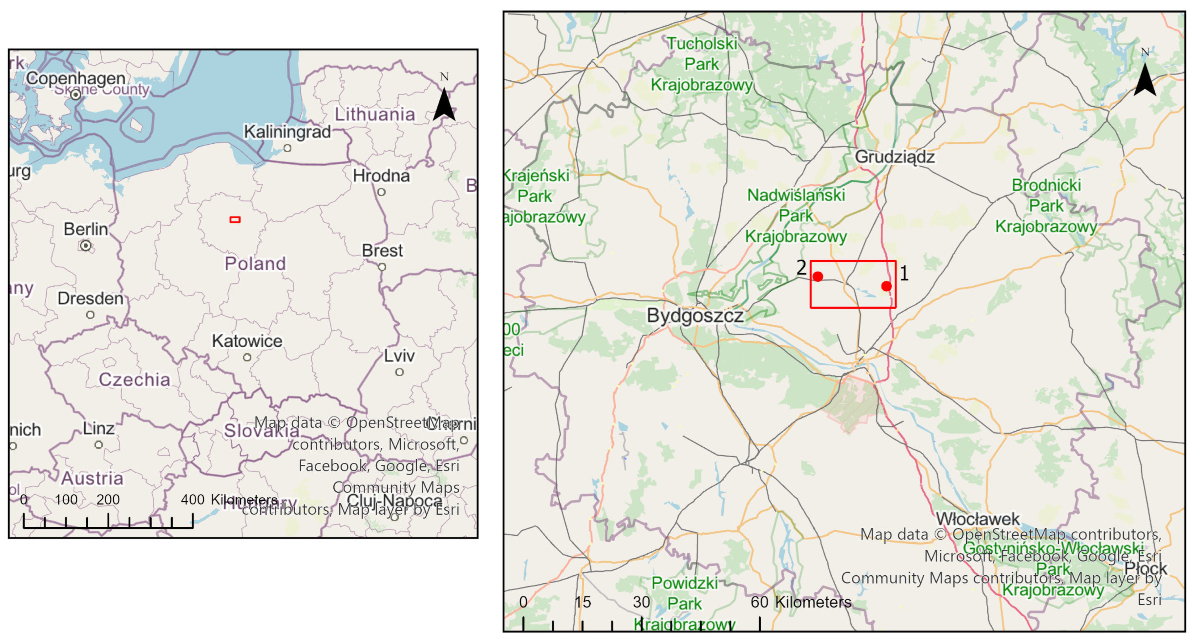
The research area selected for this study includes relics of megalithic tombs from the Funnel Beaker culture, as shown in
Figure 1. The first site is located in Dźwierzno, Chełmża municipality, and is designated as the archeological site Dźwierzno st. 60 AZP 36-45/204. It was discovered in 2019 by J. Czerniec (
Figure 1, No. 1) through the analysis of orthophoto maps from the PZGiK database [
46]. This site represents a Kujavian-type tomb, of which numerous examples were recorded in the Chełmno Land during the 19th century [
47]. Trial verification research conducted in 2019 revealed significant destruction of the tomb [
46].
Another example of a Kujavian-type tomb is located in Trzebcz Szlachecki, Kijewo Królewskie municipality, and is designated as the archeological site Trzebcz Szlachecki 32 AZP 36-42/115 (
Figure 1, No. 2). This tomb was excavated in the second half of the 19th century by G. Ossowski [
48]. As with the previous tomb, the above-ground structure was destroyed. The relic was rediscovered in 2021 by J. Czerniec, again through orthophoto map analysis. Verification studies are currently underway at this site.
A common feature of both tombs is the destruction of their above-ground structures, which has led to the “disappearance” of their monumental forms from the landscape, making them difficult for researchers to relocate. Only soil markers remain visible on the surface, characterized by their dark color. This is due to black, organic soil originally deposited in the burial chambers by the builders, who sourced the material from marshy areas. After the stone linings were dismantled and the earthen mounds dispersed, these layers gradually became exposed through long-term plowing, eventually becoming visible on the surface.
To illustrate this phenomenon, Sentinel-2 satellite data acquired on 21 June 2021, are presented, including both natural color composition (RGB) and processed variants: false color composite (FCC), NDVI and NDWI indices, soil moisture index, and a normalized RGB composite. In each image, black arrows indicate the location where anomalies corresponding to the tombs can be observed (
Figure 2a). In addition, an orthophoto map with a resolution of 5 cm is provided, allowing for the precise localization of the studied feature. Due to its high resolution, the tomb can be clearly identified in the field. This orthophoto map serves as a valuable supplement to the documentation, supporting the spatial interpretation of the tomb (
Figure 2b). It is acknowledged that the anomalies are difficult to identify without detailed spectral analysis, underscoring the need for machine learning-assisted interpretation.
This compilation aims to visualize and demonstrate how tombs may appear in satellite imagery, even in the absence of clearly defined surface features. The distinctive spectral properties of the soil used to fill the burial chambers—particularly its differing moisture content and coloration—which enabled their detection under specific spectral and seasonal conditions. The two tombs were selected based on their confirmed archeological classification, availability of archival and high-resolution satellite data, and representativeness of low-relief, eroded megalithic structures typical for the region. Their accessibility for field validation further justified their inclusion in this study.
2.2. Data Acquisition and Preprocessing
The satellite data were acquired from the Sentinel-2A satellite. The Sentinel mission, launched as part of the Copernicus program and operated by the European Space Agency (ESA) enables the acquisition of multispectral images of the Earth’s surface, covering the visible, red-edge, near-infrared (NIR), and shortwave-infrared (SWIR) bands. With a five-day imaging cycle and relatively high spatial resolution, this mission provides an excellent source of multispectral satellite imagery. Sentinel-2 satellites capture images at different spatial resolutions depending on the spectral band. For the visible and near-infrared bands, images are collected at a 10 m pixel size; for the red-edge and SWIR bands, the ground sampling distance (GSD) is 20 m (
Table 1).
The coastal aerosol and water vapor bands (B1 and B9–B10) have a pixel size of 60 m. Data from 2017 to 2020 were used in this study. For each year, all images with maximum cloud cover ≤20% were selected, resulting in a dataset of 209 images over the four-year period with suitable interpretive quality. This threshold was adopted based on common practice in remote sensing applications and preliminary empirical assessment. Images with higher cloud coverage often contained partial obstructions or cloud shadows that interfered with vegetation index calculations and hindered the identification of archeological anomalies. The ≤20% limit provided a practical trade-off between image availability and analytical reliability. Vegetation indices were calculated from the collected imagery, focusing on those potentially relevant to detecting archeological features. The most widely used index for assessing vegetation is the
NDVI [
49]:
NDVI is correlated with biomass and chlorophyll content and ranges from −1 to 1. Values below 0.2 indicate non-vegetated surfaces (e.g., built-up areas, bare soil, water, or snow). Values between 0.2 and 0.4 denote sparse vegetation, while values above 0.4 suggest the presence of healthy, green vegetation. Higher values correspond to greater biomass and healthier vegetation.
To improve surface water detection, two additional indices were used. The first is the
NDWI, which uses green and
NIR bands:
NDWI, proposed by McFeeters [
50], is used to detect and monitor surface moisture changes, with values ranging from −1 to 1. Values between 0.2 and 1 correspond to water bodies, those from 0 to 0.2 indicate flood-prone areas with high surface moisture, values from −0.3 to 0 represent moderately dry conditions, and values below −0.3 are indicative of drought.
Another relevant index is the Normalized Difference Moisture Index (
NDMI), which utilizes the
NIR and shortwave-infrared (SWIR) bands to assess moisture content.
NDMI reflects the water content present in plant tissues. The SWIR band is sensitive to changes in both plant water content and the spongy mesophyll structure, whereas
NIR reflectance is influenced by the internal structure and dry matter content of leaves but is not affected by water content. By combining
NIR and SWIR, the index minimizes variations caused by internal leaf structure and dry matter, thereby improving the accuracy of vegetation water content estimation. For Sentinel-2 data, the
NDMI is calculated as follows:
A detailed interpretation of this index distinguishes up to ten ranges, where a value of −1 corresponds to bare soil and a value of 1 represents dense vegetation with no water stress. The intermediate ranges are defined as follows: [−0.8, −0.6)—almost no vegetation; [−0.6, −0.4)—very-poor vegetation; [−0.4, −0.2)—low vegetation, either dry or wet; [−0.2, 0)—moderately low vegetation with either high or low water stress; [0, 0.2)—medium vegetation with high water stress or medium–low vegetation with low water stress; [0.2, 0.4)—medium–high vegetation with high water stress or medium vegetation with low water stress; [0.4, 0.6)—high vegetation with no water stress; [0.6, 0.8)—very-high vegetation with no water stress.
Based on the publication by [
51], the Normalized Archeological Index (
NAI) was also included, and was calculated using the following formula:
This index was proposed to enhance the visibility of subsurface features by exploiting their spectral contrast with the surrounding soil and vegetation. According to the authors, NAI facilitates the detection of buried archeological remains and is therefore considered valuable for studies focusing on tomb identification.
Meteorological data were obtained from the Integrated Surface Database (ISD) [
52], a global repository of hourly meteorological observations compiled from multiple sources and standardized into a uniform format. The nearest meteorological station to the archeological sites was located in Toruń (station code: 123767). This station was selected due to its geographic proximity to both the study sites (within ~30 km) and the completeness of its historical records during the study period (2017–2020). Given the low topographic variation in the region and the relatively homogeneous climatic conditions, the Toruń station was deemed representative for capturing local environmental variability relevant to vegetation dynamics and soil moisture. Data were retrieved using the worldmet package in R [
44], including air temperature (tt), dew point temperature (dp), relative humidity (rh), visibility (vis), wind speed (ws), precipitation (precip), and atmospheric pressure (pres). Observations from 2016 to 2020 were aggregated into weekly and monthly averages, with total precipitation computed for the same periods. These meteorological datasets were then integrated with Sentinel-2 imagery to examine the relationship between site visibility and prevailing meteorological conditions. Each satellite image was temporally aligned with the nearest weekly and monthly meteorological aggregates from the Toruń station, assuming regional representativeness due to geographic proximity.
2.3. Developing the ML Model
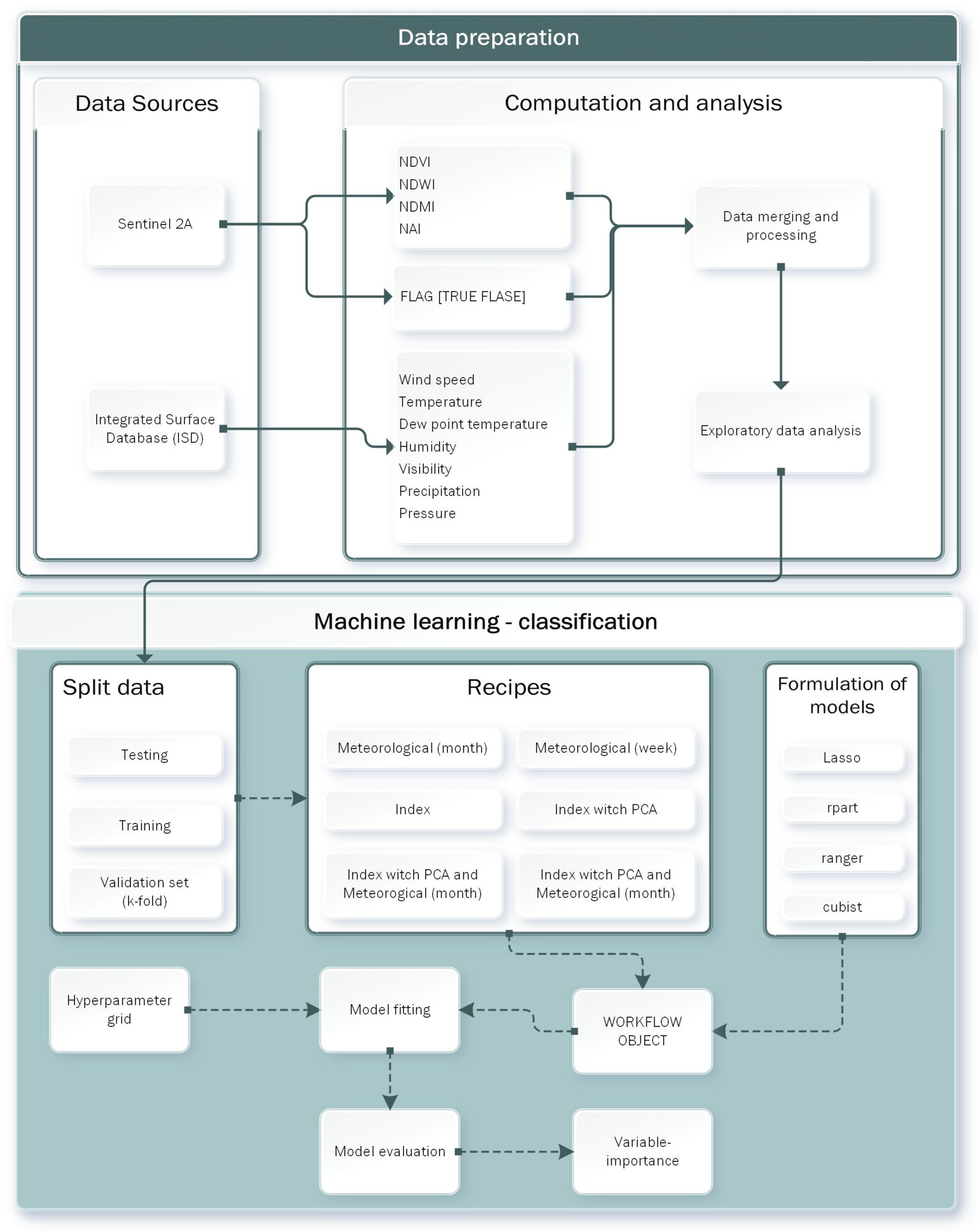
The research workflow is presented in
Figure 3. The process of data acquisition and preparation is described in
Section 2.2. The initial analytical step involved data exploration. The primary objective of the exploratory data analysis was to identify which variables were most relevant for constructing a predictive model of archeological site visibility. Graphical methods and basic descriptive statistics were employed, including sample means with 95% confidence intervals and Spearman’s rank correlation coefficient. The bootstrap method [
53] was used to compute the 95% confidence intervals. As the explanatory variables did not follow a normal distribution, robust methods appropriate for non-normally distributed data were applied.
To develop optimal algorithms, the workflow followed the guidelines of the tidymodels framework [
54]. All analyses were implemented in the R programming language [
55] using Posit IDE [
56] and Quarto technology [
57]. The dataset was initially divided into training and test sets, maintaining the proportional representation of the target variable (flag: True–visible and False–not visible), thereby preserving the original class distribution. Given the relatively small sample size (209 observations), 10-fold cross-validation was applied. Prior research suggests that 10-fold stratified cross-validation offers a good balance of low variance and high result stability for model tuning [
58].
Four classification algorithms were applied as follows: LASSO logistic regression (glmnet) [
59], decision trees (rpart) [
60], random forest (ranger) [
61], and gradient boosting (xgboost) [
62].
LASSO logistic regression (Least Absolute Shrinkage and Selection Operator) combines logistic regression with LASSO regularization to improve model performance and mitigate overfitting. Logistic regression models the relationship between a binary dependent variable and a set of independent variables by predicting class probabilities through a logistic function. The LASSO penalty, based on the sum of the absolute values of the regression coefficients, facilitates variable selection by shrinking less relevant coefficients to zero. This reduces model dimensionality, improves interpretability, and minimizes overfitting risks [
59,
63]. The regularization parameter λ was tuned using 10-fold stratified cross-validation, guided by an initial regularization path. The hyperparameter tuning process was integrated into the tidymodels framework, optimizing the area under the ROC curve (AUC) and being validated using other metrics, including the Matthews Correlation Coefficient (MCC) and F1-score, to ensure balanced model performance.
The decision tree method, implemented via rpart (Recursive Partitioning and Regression Trees), partitions the dataset into homogeneous subsets. Each decision tree consists of internal nodes, branches, and terminal nodes (leaves) representing class-specific observations. For classification, splits are determined by the Gini Index. The tree grows until a minimum number of observations per node is reached. However, decision trees are prone to overfitting and sensitive to small sample sizes [
64].
The random forest algorithm, implemented via ranger, is an ensemble approach based on decision trees that improves prediction accuracy and stability [
61,
65]. It constructs multiple trees on bootstrapped data subsets and aggregates their outputs through majority voting. Its strengths include robustness to multicollinearity, ability to handle heterogeneous data types, and tolerance for missing values. However, it requires tuning of multiple hyperparameters, has higher computational demands, and exhibits lower interpretability.
Gradient boosting, implemented via xgboost, builds an ensemble model in a sequential manner where each new tree corrects the residuals of the previous ones. It incorporates built-in regularization techniques to prevent overfitting. Although parallel computation is supported, the model remains relatively slower due to the sequential construction process. Moreover, excessive iterations can lead to overfitting if not adequately regulated [
62,
66].
Multiple data preparation workflows were designed to assess how model performance varied based on the inclusion and selection of independent variables.
Table 2 summarizes these workflows, which aim to identify which variables are most effective for predicting the visibility of archeological sites and whether the inclusion of meteorological data improves performance. Due to the high correlation among NDVI, NDWI, NDMI, and NAI indices, the “index” workflow was limited to three variables to avoid multicollinearity. Strongly correlated predictors can lead to unstable coefficients, wider confidence intervals, excessive unnecessary model complexity, and reduced interpretability. Some supervised learning algorithms may also arbitrarily select one correlated feature over another [
59,
60]. To address multicollinearity, Principal Component Analysis (PCA) was applied to the vegetation indices (NDVI, NDWI, NDMI, and NAI) in the selected workflow. Data transformations included binarization of categorical variables and removal of zero-variance features. For LASSO logistic regression, input variables were also normalized.
The optimization of supervised learning algorithms employed racing methods [
54,
67], which evaluated all models on a subset of the data and discarded underperforming hyperparameter configurations. Performance differences were assessed using ANOVA to identify statistically significant inferior combinations. This method reduces computational costs while maintaining statistical validity.
A comparative evaluation of the models was conducted using the following performance metrics:
AUC (Area Under the ROC Curve): Measures the ability to discriminate between classes.
MCC (Matthews Correlation Coefficient): Provides a balanced evaluation using all elements of the confusion matrix.
F1-score: Harmonic means of precision and recall.
KAP (Cohen’s Kappa): Measures agreement while adjusting for chance.
While AUC and F1-score range from 0 to 1 (with 1 indicating perfect classification), MCC and KAP range from −1 to 1 (with 1 indicating perfect agreement and 0 representing random classification). These metrics are especially informative in imbalanced classification scenarios.
An exploratory analysis of selected models was performed to determine which independent variables most influenced predictions. This variable importance analysis, conducted using the DALEX package [
68,
69], improves model transparency and can inform further model refinement.
3. Results
3.1. Statistical Characteristics of the Data
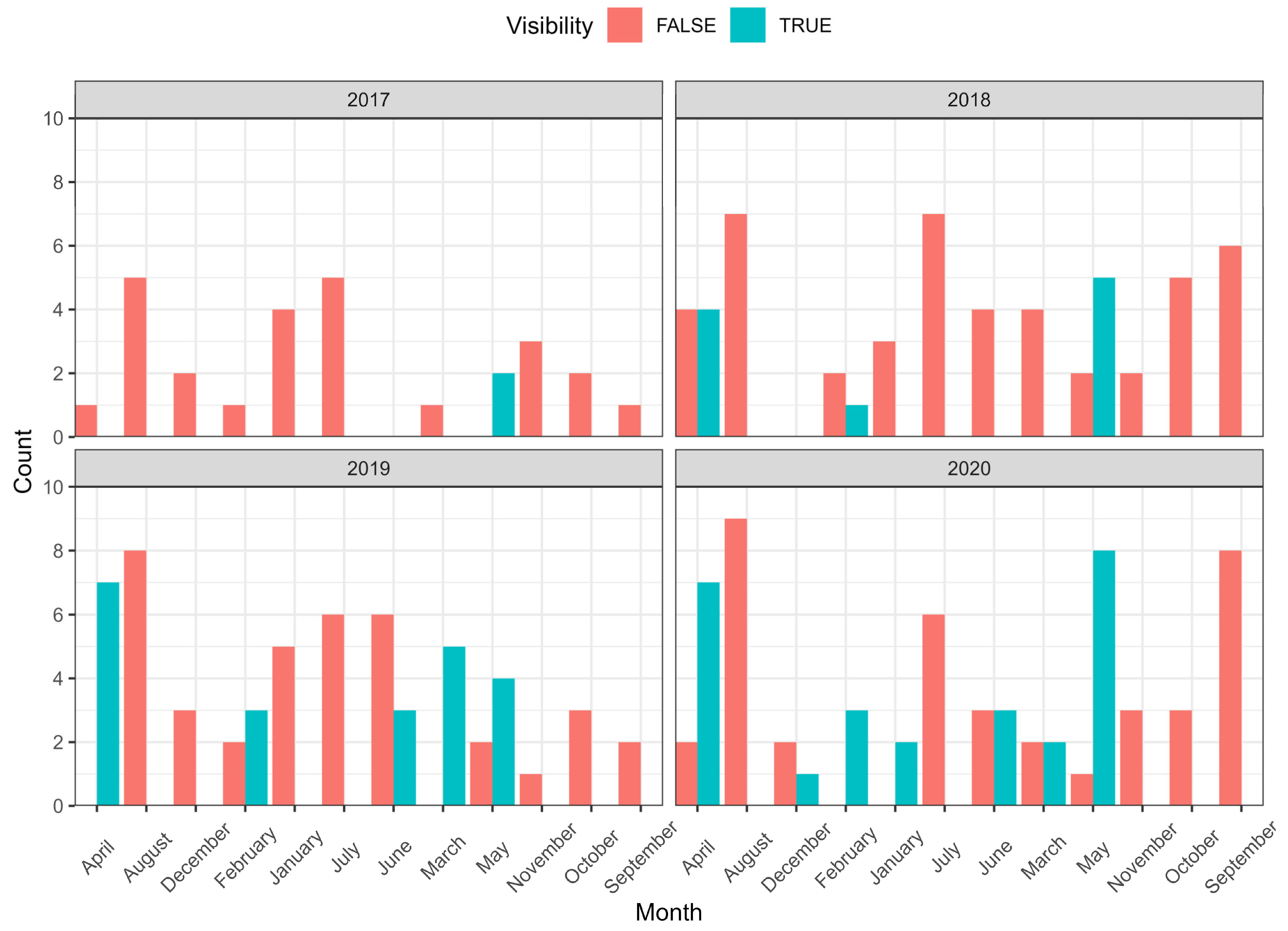
The dataset comprises 209 observations, which were analyzed to evaluate the potential for identifying archeological sites in satellite imagery. Visibility labels (TRUE/FALSE) were assigned to each image based on expert manual interpretation, incorporating spectral anomalies and prior knowledge of the sites. In 28.7% of the cases, the presence of a site could be clearly confirmed, indicating the meaningful, though limited, potential for remote sensing in such analyses. Positive identifications occurred predominantly between January and May (
Figure 4), likely due to low vegetation cover and moderately dry soil conditions in the study area (
Figure 5). The absence of dense vegetation enhances the visibility of archeological features, which often appear as variations in soil color or subtle changes in texture. From July onward, a sharp annual increase in NDVI values was observed, indicating vigorous vegetation growth. Simultaneously, a decline in NDWI values was recorded, reflecting progressive soil moisture depletion and increasing drought conditions (
Figure 5). Under these circumstances, archeological site detection becomes significantly more challenging as dense vegetation obscures subtle land cover differences and the soil loses the contrasting properties that facilitate site identification.
The substantial interannual variation in the results reflects changes in the identifiability of archeological sites, which are directly influenced by meteorological conditions—particularly annual precipitation totals and temperature fluctuations. These factors affect vegetation dynamics and soil moisture levels, both of which are crucial for site visibility in satellite imagery.
An additional limitation of the analysis was the exclusion of certain images due to high cloud or snow cover, which rendered observation verification impossible. This issue was particularly pronounced in 2017, when a significant number of images were unsuitable for analysis. Moreover, not all years exhibited a high frequency of positive identifications. The highest detection rates occurred in 2019 and 2020. This pattern underscores the impact of meteorological variability—including temperature, precipitation, and humidity—on the visibility of archeological sites in satellite imagery (
Figure 6).
The results presented in
Figure 5 indicate statistically significant differences in the mean values of the NAI, NDMI, NDVI, and NDWI indices depending on whether an archeological site was visible or not. This is evidenced by the non-overlapping 95% confidence intervals observed for each year. Mean NDVI values ranged from 0.18 to 0.20 when sites were visible (flag = TRUE), whereas for flag = FALSE, values ranged from 0.36 to 0.82. This suggests that archeological sites tend to be visible when surface vegetation is sparse. In contrast, sites are generally not visible when vegetation is moderate (NDVI > 0.2) or dense (NDVI > 0.6). Low NDVI values reflect vegetation stress, which enhances the detectability of subsurface features. The NDWI further supports the relationship between site visibility and soil moisture. Sites were visible at average NDWI values between −0.29 and −0.32, indicating moderately dry conditions. In contrast, extremely low NDWI values—typically associated with severe drought—corresponded to site invisibility, suggesting that very low soil moisture inhibits the detection of archeological features. A similar pattern was observed at NDMI values between −0.15 and −0.20, consistent with low vegetation and minimal water stress. The NAI, as proposed by [
51], also exhibited characteristic values for visible sites (flag = TRUE), ranging from 0.06 to 0.08.
These findings demonstrate the potential to predict, with high probability, the satellite images in which archeological sites are likely to be visible, based on these indices. The average monthly values of meteorological parameters—wind speed ws, temperature tt, visibility vis, and precipitation precip)—varied throughout the study period (
Figure 6), and in many cases, these averages differed significantly. Notably, positive identifications of archeological sites occurred only from January to July.
Figure 5 reveals a near-complete absence of precipitation in January 2017 and February 2018, accompanied by sub-zero temperatures, under which site visibility was not achieved. In contrast, the same months in 2019 and 2020 experienced higher rainfall and temperatures, corresponding with successful identifications.
Of particular interest is wind speed (ws), which was significantly lower in 2017 and 2018 during periods when the sites were not visible. Whether wind speed directly affects the visibility of archeological sites remains unclear and warrants further investigation, which will be addressed in future research. Other meteorological variables—including wind direction, humidity, and atmospheric pressure—did not exhibit consistent patterns over the study period and were therefore excluded from further analysis.
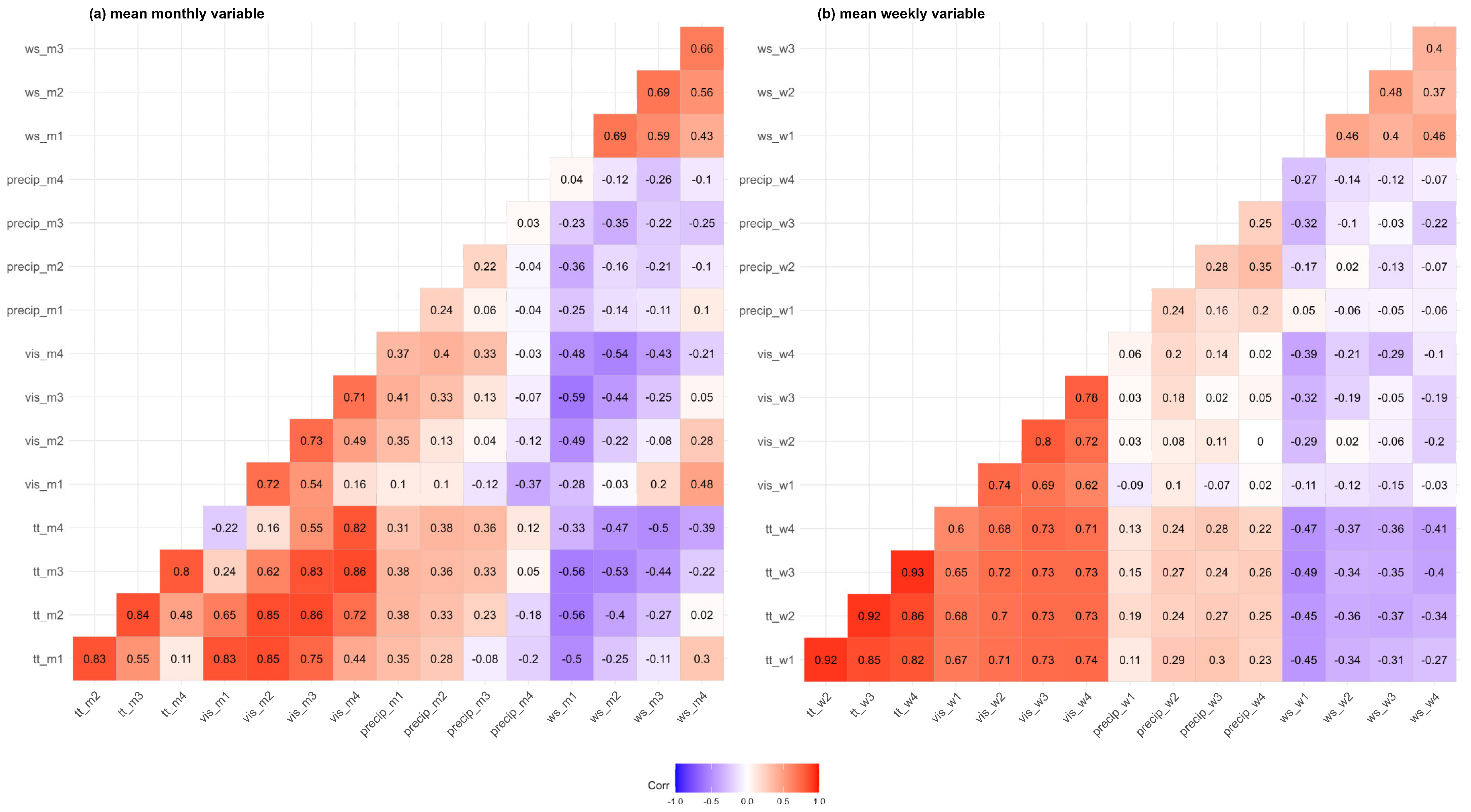
3.2. Dependency Analysis
Figure 7 presents the correlation matrix for selected meteorological variables, averaged over monthly and weekly periods.
Spearman’s rank correlation was applied due to the non-normal distribution of the variables. Several meteorological parameters exhibited temporal dependencies, particularly temperature (tt), visibility (vis), and wind speed (ws). The strength of these correlations generally decreased with increasing temporal separation. For example, the average monthly temperature in the month immediately preceding the satellite image (tt_m1) was strongly correlated (r = 0.83) with that of the previous month (tt_m2). However, the correlation declined substantially for earlier months, with a Spearman correlation of r = 0.11 between tt_m1 and tt_m4. In contrast, monthly precipitation totals showed minimal interdependence, with correlation coefficients below |0.22|, indicating weak or no correlation between precipitation values across different months. For weekly averages, a similar weak correlation was observed for average weekly wind speeds (r < |0.48|). The remaining meteorological variables displayed similar patterns to those observed in the monthly averages. This analysis suggests that the values of certain meteorological parameters exhibit strong dependence on recent historical conditions. Consequently, historical data for these variables may provide valuable predictive information regarding the visibility of archeological sites in satellite imagery.
3.3. Evaluation of Model Accuracy
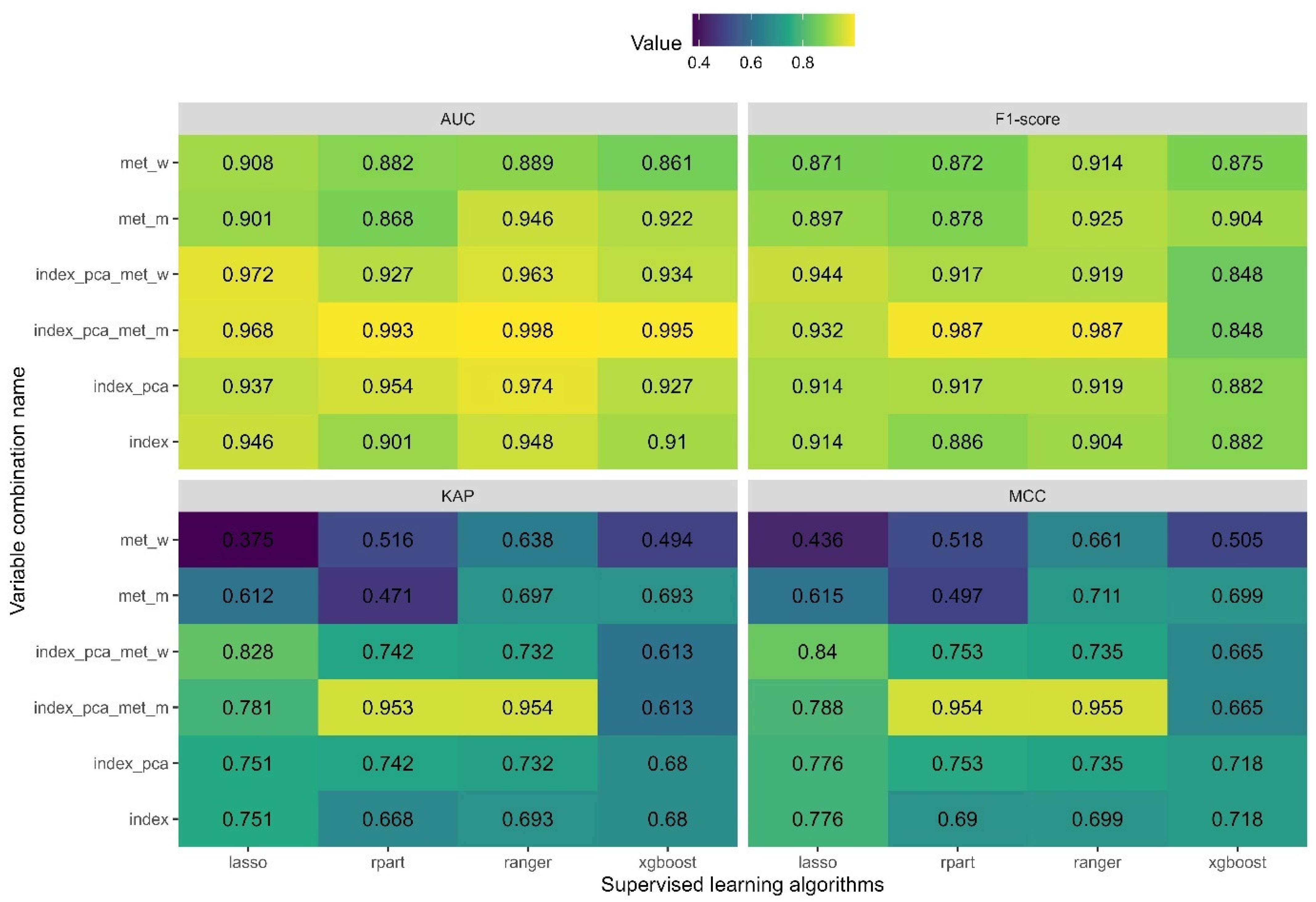
The results presented in
Figure 8 indicate that all models—regardless of the algorithm or input dataset—achieved very high performance on the test dataset, with both the AUC and F1-score exceeding 0.85. These findings demonstrate that the visibility of archeological structures can be predicted accurately, precisely, and sensitively using a combination of satellite imagery and meteorological data. The most effective models for identifying the visibility of archeological structures were obtained using decision tree algorithms (rpart) and random forest (ranger) when both vegetation indices and meteorological variables were included. Based on the AUC, KAP, and MCC metrics, the random forest algorithm yielded the highest overall performance. However, the F1-score revealed comparable predictive accuracy for both algorithms. As a result, it is not possible to determine definitively which algorithm is superior based solely on these metrics. Therefore, additional analyses of variable importance were conducted in
Section 3.4 to provide a deeper understanding of model behavior and decision-making.
Models developed using only meteorological data (met_w, met_m) exhibited lower accuracy than those based on combined explanatory variables. Nevertheless, they achieved a minimum predictive accuracy of 87% in determining whether archeological structures would be visible. This is particularly valuable for planning archeological surveys aimed at detecting existing structures via aerial imagery. Estimating the probability of site visibility using historical meteorological data enhances the efficiency of aerial surveys and reduces the costs associated with flights conducted during suboptimal periods. The accuracy metrics (
Figure 8) clearly indicate that the random forest algorithm, when applied to average monthly meteorological data, was the most effective among the supervised learning models based solely on meteorological inputs. This approach yielded the highest values of AUC, F1-score, KAP, and MCC. Slightly lower performance was observed for the gradient boosting algorithm (xgboost), also applied to average monthly meteorological parameters. Consequently, variable importance analyses were also conducted for these models.
3.4. Analysis of Variable Importance
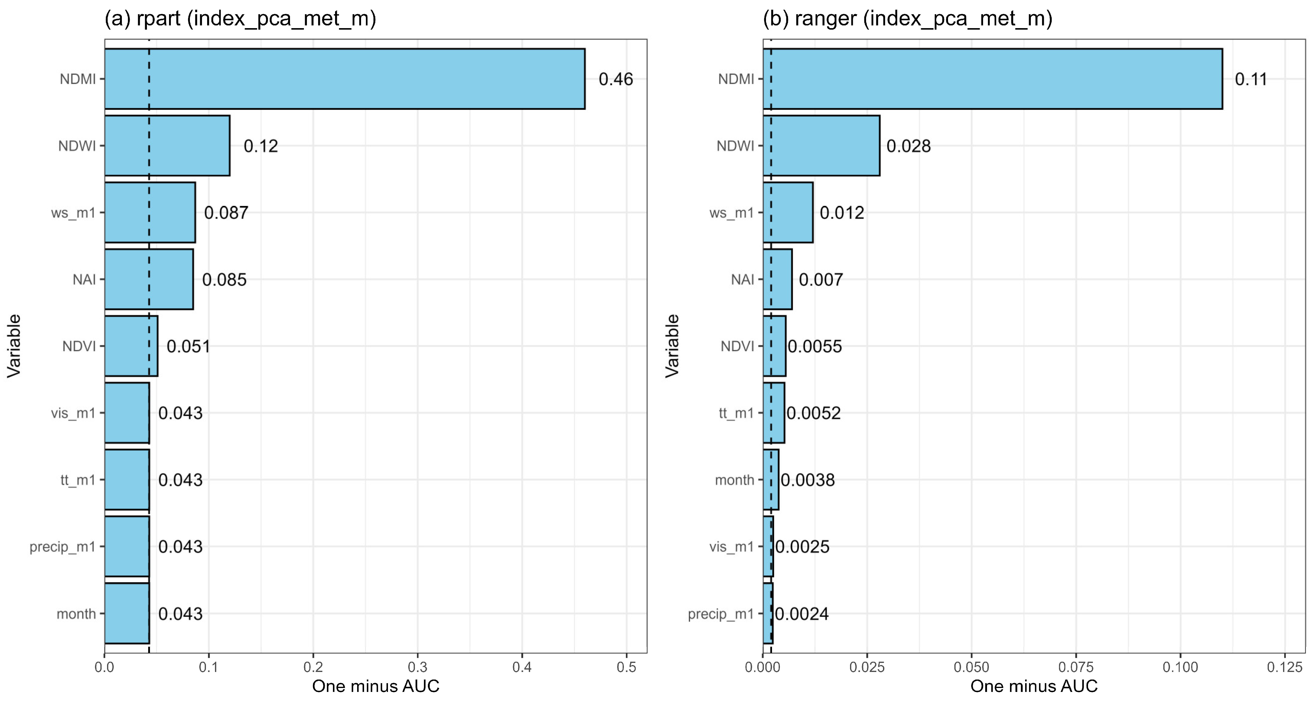
Variable importance was assessed using the permutation-based method implemented in the DALEX package. For each predictor, values were randomly permuted while keeping the remaining features fixed, and the resulting decrease in AUC was recorded. The values reported in
Figure 9 represent one − the AUC after permutation, reflecting the reduction in predictive accuracy attributable to each feature. A higher ‘1–AUC’ value indicates a greater contribution of the variable to the model’s performance.
Figure 9 illustrates the importance of individual explanatory variables for selected decision tree (rpart) and random forest (ranger) models, in which PCA-based dimensionality reduction was applied to both indices and meteorological variables. In the decision tree model, NDMI emerged as the most significant variable. Exclusion of this variable led to predictions no better than random, indicating a strong dependence on a single predictor, despite the inclusion of multiple variables and the application of dimensionality reduction. This highlights a classic case of over-reliance on a dominant variable. To address the apparent discrepancy between the decision tree’s reliance on NDMI and the random forest’s balanced use of all variables, it is important to emphasize the differences in modeling approaches. Single decision trees (e.g., rpart) select splits based on local optima (e.g., Gini impurity reduction), which can exaggerate the perceived importance of certain variables. In contrast, random forests aggregate predictions across hundreds of trees, each trained on bootstrapped data and random feature subsets. This ensemble approach inherently accounts for variable interactions and reduces overfitting to individual predictors. Although NDMI remained critical in both models, its dominance in the decision tree reflects algorithmic bias toward locally optimal splits, whereas the random forest’s permutation-based importance scores (
Figure 9b) reveal more distributed and complementary contributions from all variables.
Notably, in the rpart model, most meteorological variables were found to be insignificant. The removal of visibility (vis), temperature (tt), precipitation (precip), and month, did not affect predictive performance. The only significant meteorological predictor was wind speed (ws), specifically in the rpart model using the index_pca_met_m dataset. In contrast, all variables in the corresponding random forest model were deemed significant, as indicated by 1–AUC values exceeding the model’s baseline threshold of 0.0014. Furthermore, the distribution of importance scores was more balanced. While NDMI remained the most influential variable, its removal did not reduce performance to random levels, indicating greater robustness of the random forest model. These findings support the conclusion that the random forest algorithm is better suited for predicting the visibility of archeological structures in satellite imagery.
The role of wind speed in accelerating soil evaporation and influencing plant water stress is well-documented [
70]. Studies using high-resolution meteorological modeling confirm that increased wind enhances evaporation and transpiration rates by 12–18% in exposed landscapes, leading to rapid surface drying [
71]. This accelerated moisture loss can intensify contrasts in water retention between subsurface archeological features and surrounding undisturbed soils. Contemporary archeological remote sensing research highlights that wind-mediated moisture changes create temporal windows of enhanced feature visibility, especially in arid and semi-arid regions where vegetation stress is most pronounced [
72,
73].
Figure 10 presents the variable importance results for the random forest and gradient boosting (xgboost) models using meteorological data from the preceding three months. In the xgboost model, average air temperature from two and three months prior (tt_m2, tt_m3) emerged as the most significant variables. Wind speed (ws_m1, ws_m2), visibility (vis_m1, vis_m2), and precipitation (precip_m1) also contributed meaningfully, whereas the remaining variables were deemed insignificant. Conversely, the random forest model (met_m) found all variables to be significant, with no single variable exerting a dominant deterministic influence. Given the known interdependencies among meteorological variables via underlying physical processes, the random forest approach is considered more robust and appropriate for this application.
4. Discussion
The previous studies have primarily focused on detecting patterns of archeological site structures using deep learning methods. For instance, convolutional neural networks (CNNs) have been applied to identify princely tombs on the border of Kazakhstan and China [
74], Qanat shafts in Iraq [
75], and various archeological sites in Poland [
75], based on visible and near-infrared imagery. Similarly, research conducted in Mexico and Guatemala has aimed to identify specific pixels in satellite images that correspond to archeological structures, employing various machine learning algorithms [
76]. These studies concentrated exclusively on detecting discrete archeological features within satellite imagery. The models developed generally exhibited high precision and sensitivity, with reported F1-scores of 0.705 [
74], 0.76 [
75], 0.99 [
76], and 0.94–0.95 [
77]. A commonality among these studies is their sole reliance on satellite imagery.
In contrast to the studies by [
16,
78], the present research focused on analyzing satellite-derived vegetation indices—NDWI, NDVI, NDMI, and NAI—in conjunction with historical meteorological data. Although direct soil moisture data were not available, proxies such as precipitation, relative humidity, temperature, and wind speed were employed to characterize its temporal variability. For example, precipitation contributes directly to the increase in soil moisture, whereas high temperatures and wind speed accelerate evapotranspiration, reducing surface water content. Relative humidity modulates evaporation rates and influences vegetation stress responses. These meteorological parameters thus serve as indirect indicators of soil moisture dynamics, which are crucial for enhancing the spectral contrast between buried archeological features and their surroundings. The interaction of these variables with vegetation indices enabled the machine learning models to infer periods when soil moisture conditions were most conducive to feature visibility.
The proposed approach differs by enabling preselection of existing LANDSAT imagery, thereby facilitating the automatic exclusion of unsuitable images and assessing whether, based on historical meteorological conditions, it is appropriate to conduct aerial surveys during a given period. This simplified methodological framework yielded models with high precision and sensitivity, achieving an F1-score of 0.987 when combining indices with meteorological data. Even when using meteorological data alone, the models performed well, with an F1-score of 0.925.
A key limitation of this and similar studies is the issue of spatial representativeness. The algorithm developed here was trained on data from a single archeological site. As noted by [
76], model performance can vary substantially by location, necessitating the acquisition of data from more diverse regions. Nevertheless, the strength of the present study lies in its extended temporal scope. Unlike previous studies, this research utilized hundreds of images collected over a four-year period (2017–2020), enabling the correlation of vegetation indices with meteorological conditions and yielding a more robust model that accounts for environmental variability.
The methodology proposed offers considerable potential to accelerate archeological investigations. Firstly, models based on combined indices and meteorological data can identify satellite images that are more likely to reveal archeological structures, effectively filtering large datasets and focusing expert analysis. Secondly, meteorological data alone can guide the optimal timing of aerial campaigns to acquire multispectral data, including LiDAR, thereby reducing overall research costs.
Despite the robust performance of the methodology in identifying optimal detection conditions, several limitations must be acknowledged. First, the geographic specificity of the dataset—limited to tomb sites in a localized area—raises concerns about model generalizability. Results derived from a small number of known sites may not transfer well to regions with differing environmental conditions or archeological features, a challenge also recognized in prior studies of site-specific ML applications. Second, the reliance on data from a single meteorological station limits the spatial representativeness of environmental variables, potentially introducing biases when applying the model to larger geographic scales. Although the models achieved high performance, including on the independent test set, their generalizability can only be fully confirmed through validation on datasets from other regions or time periods.
These limitations reflect broader methodological challenges in archeological machine learning, where locally trained models often lack cross-regional applicability. Future research should therefore prioritize testing the framework in geographically diverse areas, incorporating spatially distributed climate data from reanalysis products such as ERA5-Land to capture microclimatic variability more accurately. Additionally, integrating advanced vegetation metrics—such as the Enhanced Vegetation Index (EVI)—or hyperspectral features could further enhance model sensitivity to subtle spectral contrasts, particularly in arid or densely vegetated regions where indices such as NDVI or NDMI may saturate.
Despite its limitations, this study advances the field by systematically integrating meteorological and satellite-derived vegetation data. The use of a four-year dataset (2017–2020) and the focus on environmental interactions provides a replicable framework for applying this methodology to other archeological contexts, particularly where traditional spectral analysis alone proves insufficient. This dual-data approach represents a conceptual shift away from purely imagery-based detection and introduces practical tools for optimizing survey timing across diverse climatic zones.
5. Conclusions
This study presented a novel methodology for improving the prediction of archeological site visibility in satellite imagery by integrating spectral indices with meteorological parameters within a machine learning framework. Focusing on megalithic tombs associated with the Funnel Beaker culture in Poland, the research demonstrated that the combined use of NDVI, NDWI, NDMI, and NAI with weather data—particularly wind speed and temperature—significantly enhances predictive performance compared to spectral indices alone.
Among the machine learning algorithms evaluated, decision trees and random forests consistently yielded the highest classification accuracy, with F1-scores reaching 0.987 and AUC values approaching 0.998. These findings underscore the potential of incorporating environmental context into archeological remote sensing applications. The capacity to predict site visibility under varying environmental conditions facilitates the optimization of observation schedules and the preselection of satellite imagery, thereby reducing operational costs and improving the efficiency of archeological surveys.
The most accurate predictions were obtained during periods characterized by moderate precipitation followed by drying phases, which altered surface soil moisture, as well as short-term fluctuations in temperature, wind speed, and humidity, which induced vegetation stress and influenced spectral reflectance. These dynamic environmental conditions increase the spectral contrast between disturbed and undisturbed soils, thereby enhancing the detectability of subsurface archeological features.
Despite the promising results, the study is constrained by the spatial specificity of the dataset, which includes a limited number of tomb sites within a localized area. This raises concerns regarding the generalizability of the models, as results derived from only two known sites may not be applicable to regions with different environmental or archeological characteristics. Furthermore, the reliance on meteorological data from a single weather station limits the spatial representativeness of the environmental variables. Future research should focus on validating the proposed methodology in diverse geographic settings, incorporating spatially distributed climate data (e.g., from reanalysis products), and exploring the integration of more advanced vegetation metrics, such as the Enhanced Vegetation Index (EVI) or hyperspectral features.
In conclusion, the findings highlight the value of a multidisciplinary approach that integrates archeological knowledge, remote sensing techniques, and environmental data science to advance the detection and monitoring of buried heritage features under varying landscape and climatic conditions.


 ,
, 


