VOX-LIO: An Effective and Robust LiDAR-Inertial Odometry System Based on Surfel Voxels

Abstract

Accurate and robust pose estimation is critical for simultaneous localization and mapping (SLAM), and multi-sensor fusion has demonstrated efficacy with significant potential for robotic applications. This study presents VOX-LIO, an effective LiDAR-inertial odometry system. To improve both robustness and accuracy, we propose an adaptive hash voxel-based point cloud map management method that incorporates surfel features and planarity. This method enhances the efficiency of point-to-surfel association by leveraging long-term observed surfel. It facilitates the incremental refinement of surfel features within classified surfel voxels, thereby enabling precise and efficient map updates. Furthermore, we develop a weighted fusion approach that integrates LiDAR and IMU data measurements on the manifold, effectively compensating for motion distortion, particularly under high-speed LiDAR motion. We validate our system through experiments conducted on both public datasets and our mobile robot platforms. The results demonstrate that VOX-LIO outperforms the existing methods, effectively handling challenging environments while minimizing computational cost.

1. Introduction

In recent years, autonomous mobile platform technologies, including mobile robots, unmanned aerial vehicles (UAVs), and autonomous driving, have become a research hotspot in the field of artificial intelligence. In these applications, location-based, high-precision maps play a critical role. simultaneous localization and mapping (SLAM) has also gained considerable attention as a framework that can autonomously and incrementally build maps while simultaneously estimating poses.

Depending on the sensing modality, SLAM can be broadly categorized into two types: Laser SLAM and Visual SLAM. Single-sensor SLAM algorithms, such as LOAM [1] and F-LOAM [2], have been widely adopted due to their simplicity and ease of deployment. However, these approaches often struggle in complex real-world environments due to the inherent limitations of individual sensors, such as sensitivity to environmental conditions, limited observability, and reduced robustness in dynamic scenes. To address these challenges, LiDAR-inertial odometry (LIO) systems, such as Fast-LIO [3,4] and LIO-SAM [5], have been developed. These systems demonstrate strong real-time performance and computational efficiency, even on resource-constrained platforms like Raspberry Pi. Nevertheless, significant challenges persist in handling real-world uncertainties, including time synchronization errors, sensor drift, and measurement noise, which can significantly compromise the system’s accuracy and long-term consistency. These issues continue to motivate the development of more robust, scalable, and adaptable SLAM frameworks.

The fundamental principle of SLAM is fusing multi-sensor data to estimate the robot’s state. However, mobile robotic platforms are typically constrained by power consumption and hardware budgets, resulting in limited battery life and reduced computational capability compared to desktop-class systems. Moreover, multi-sensor fusion is computationally intensive and prone to cumulative errors over time, placing stringent demands on both the efficiency and accuracy of SLAM algorithms.

To address this issue, we propose a LiDAR-inertial odometry system (VOX-LIO) that combines an efficient architecture with weighted fusion on the manifold to achieve real-time, high-precision mapping on resource-constrained platforms.

In summary, our contributions are as follows:

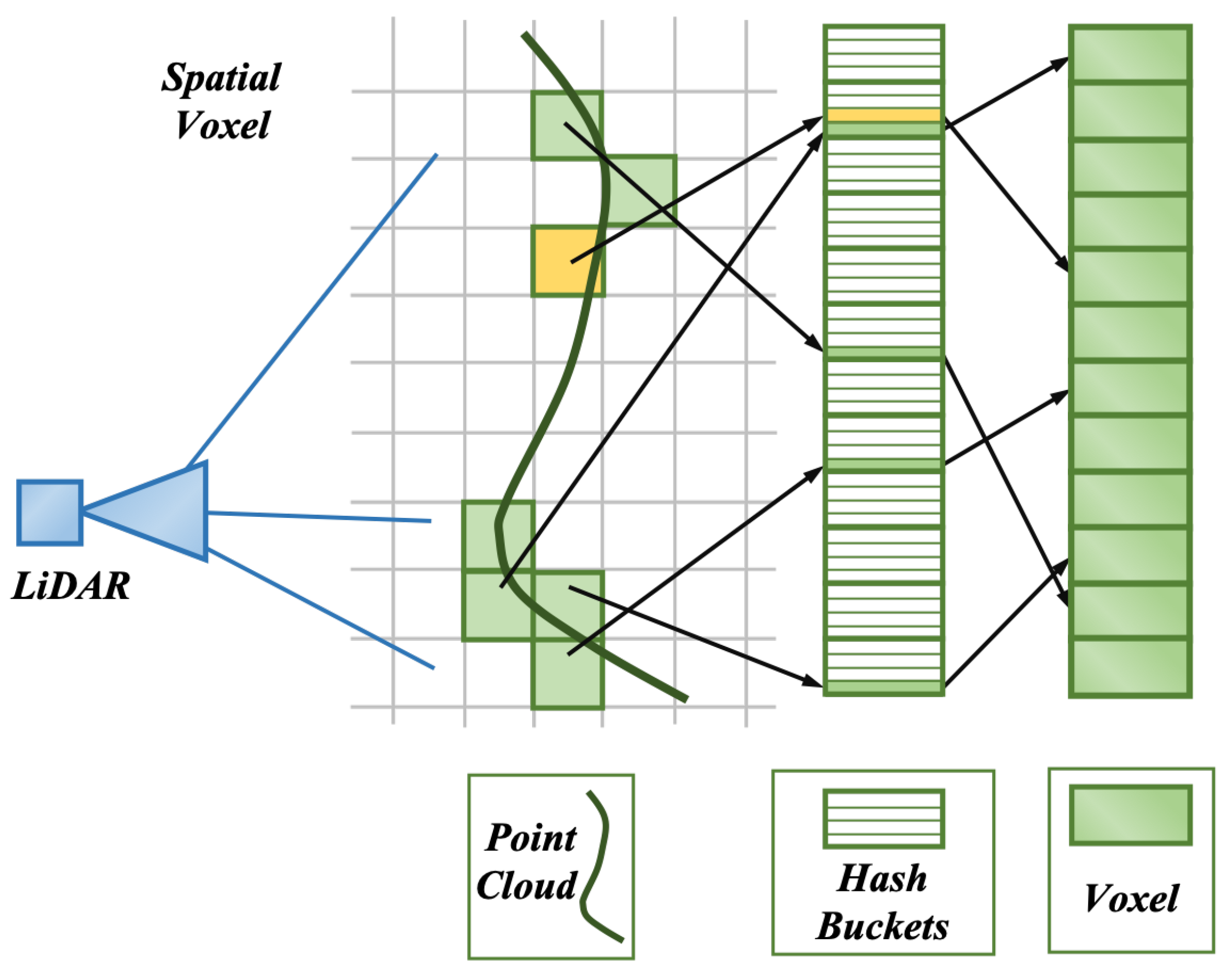
• We propose a point cloud matching strategy based on adaptive hash voxels that incorporate surfel features and planarity. This method classifies spatial voxels into surfel and common classes based on planarity. To enhance efficiency, surfels consistently observed over time are reused to constrain optimization. This approach also supports incremental refinement of surfel features within surfel voxels, enabling accurate and efficient map updates.
• We propose a weighted fusion strategy that integrates LiDAR-IMU data measurements on the manifold space. This approach compensates for motion distortion, especially during rapid LiDAR movement. To ensure stability, the fusion method may leverage robust kernel functions in conjunction with advanced optimization techniques.
• We integrate a loop closure module into VOX-LIO to enhance global consistency. Comprehensive experiments on public datasets and our robotic platforms demonstrate the system’s effectiveness in pose estimation accuracy and global map consistency. On the kitti_05 sequence, VOX-LIO reduces the mean APE by 63.9% compared to Faster-LIO, while VOX-LIOM further reduces it by 55.5% over VOX-LIO, demonstrating significant improvements in pose estimation accuracy. Furthermore, on our private dataset, the integration of the loop closure module enables VOX-LIOM to maintain globally consistent maps during extended operation.

2. Related Work

A typical LiDAR-inertial odometry (LIO) system consists of three core components: data association, map management, and sensor fusion. Loop closure and global optimization are employed to ensure global consistency of the trajectory and map.

2.1. Point Cloud Registration and Data Association

Accurate and real-time point cloud registration is essential to LiDAR-based SLAM. The classical iterative closest point (ICP) algorithm, introduced by Besl et al. [6], remains a cornerstone in geometric registration tasks. Extensions such as PL-ICP [7] and NICP [8] improve convergence rates and robustness to noise. Several other variants [9,10,11] have been proposed to enhance matching performance under challenging conditions further. The normal distributions transform (NDT) [12] improves computational efficiency and reduces matching errors, though it tends to degrade with accumulated or large-scale point clouds. LOAM [1] and LeGo-LOAM [13] incorporate geometric features and computational optimizations, leading to improved registration results.

To address the sparsity and noise in single-frame point clouds, learning-based methods have emerged. For example, SuMa [14] projects point clouds into depth images for feature extraction, while SuMa++ [15] incorporates learned semantic features. However, these approaches often face challenges in achieving real-time integration within SLAM frameworks due to high computational demands.

2.2. Point Cloud Map Management

KD-Tree [16] is widely adopted in ICP variants for nearest neighbor search due to its $O(nlogn)$ query efficiency. However, it suffers from expensive data insertion and removal operations, requiring $O\left(nlogn\right)$ for reconstruction. iKD-Tree [17] mitigates this by incrementally balancing updates and supporting submap storage, but rebalancing still incurs $O(mlogm)$ complexity, limiting its real-time performance.

Cartographer [18] employs probabilistic occupancy grids and truncated signed distance fields (TSDFs) for map representation. These approaches provide dense and accurate reconstructions but are limited by high computational overhead and limited scalability in large-scale or long-term mapping scenarios.

Despite their advantages, these map management methods face significant challenges in balancing computational efficiency, real-time update capability, and scalability, particularly in complex, large-scale, or long-duration SLAM deployments. Developing map representation and maintenance techniques that address these trade-offs remains a critical area for advancing real-time and robust SLAM systems.

2.3. Multi-Modal Sensor Fusion for State Estimation

LiDAR sensors provide accurate 3D structural information but are susceptible to motion distortion and adverse weather conditions such as rain and fog. In contrast, IMUs and cameras are lightweight and cost-effective but tend to suffer from cumulative drift over time. To overcome the limitations of individual sensors, multi-modal fusion approaches have been extensively explored.

Loosely coupled systems, such as Cartographer [18], Gmapping [19], and LeGO-LOAM [20], typically process sensor data independently before combining their outputs. Filter-based methods commonly employ extended Kalman filters (EKF) [21,22,23] or particle filters [24] for integrating sensor data. For example, Fast-LIO improves computational efficiency by introducing an optimized Kalman gain update for handling large-scale LiDAR data.

Tightly coupled fusion approaches aim to optimize measurements from multiple sensors to improve localization robustness jointly. For instance, LIO-Mapping [25] tightly fuses LiDAR and IMU data in an EKF framework to achieve reliable state estimation under degeneracy. R3LIVE [26] further incorporates visual features to improve performance in perceptually degraded environments. LIO-SAM [5] integrates IMU, LiDAR, and GPS with high robustness, though it suffers from gimbal lock issues due to Euler angle representation. Critically, IMU pre-integration remains essential for compensating motion distortion and ensuring multi-sensor temporal consistency.

2.4. Loop Closure Detection and Global Optimization

Loop closure ensures long-term global consistency by recognizing revisited places and enforcing trajectory corrections. However, real-time loop detection introduces computational and memory burdens.

Scan Context [27] encodes 3D LiDAR scans into polar grids with rotation invariance for efficient place recognition. LiDAR-Iris [28] and SPA [29] offer additional improvements in loop closure robustness and speed.

Global trajectory refinement is typically formulated as a nonlinear optimization problem over a pose graph. Classical methods such as $\sqrt{\mathrm{SAM}}$ [30] exploit sparsity in bundle adjustment for visual SLAM. At the same time, iSAM [31] achieves efficient incremental updates by exploiting the structure of the nonlinear least squares problem. These optimization strategies often operate on Lie groups (e.g., SE(3)) and require manifold-based optimization techniques to ensure consistent estimation over non-Euclidean spaces.

3. Methods

In this section, we elaborate on the complete SLAM framework, as illustrated in Figure 1. The VOX-LIO system takes LiDAR point clouds and IMU measurements as input and adopts a tightly coupled strategy to fuse the two modalities for real-time pose estimation. The raw point cloud is first downsampled via voxel filtering and then motion-compensated using integrated inertial measurement unit (IMU) data. The undistorted point cloud is aligned with the voxel submap to compute matching residuals. Constraints from IMU integration are jointly optimized with these residuals through nonlinear optimization on the manifold, resulting in high-precision pose estimates. To ensure global consistency, a loop closure module performs pose-graph-based global optimization, thereby mitigating long-term drift.

More detailed derivations of the methodology are provided in Appendix A and Appendix B.

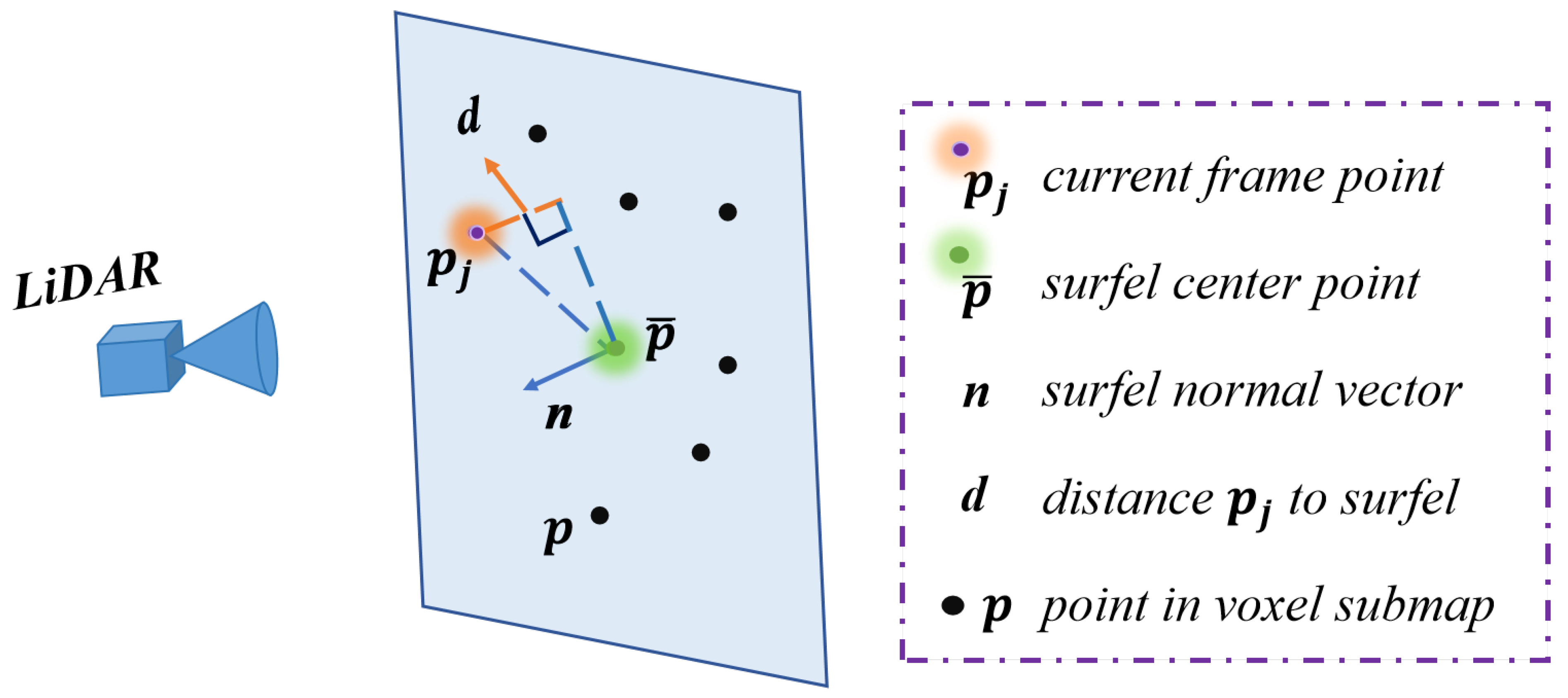
3.1. Probabilistic Model-Based Surfel Feature Fitting

3.1.1. Definition of Surfel Feature

A point cloud in the world coordinate system, denoted as ${\mathit{P}}^w=\{{\mathit{p}}_1^w,{\mathit{p}}_2^w,\dots ,{\mathit{p}}_N^w\}$, is represented by its mean $\overline{\mathit{p}}$ and variance $\mathit{A}$, as shown in Equation (1). As illustrated in Figure 2, when the points in ${\mathit{P}}^w$ lie on the same plane, they form a surfel feature characterized by the geometric center of the point cloud and the normal vector of the plane, as expressed in Equation (1).

$$\overline{\mathit{p}}={\displaystyle \frac{1}{N}}\sum _{i=1}^N{\mathit{p}}_i^w,\mathit{A}={\displaystyle \frac{1}{N}}\sum _{i=1}^N\left({\mathit{p}}_i{{\mathit{p}}_i}^T\right)-\overline{\mathit{p}}{\overline{\mathit{p}}}^T$$

(1)

By applying principal component analysis (PCA), the three-dimensional distribution of points on a plane can be reduced to two dimensions. To assess the quality of the surfel feature, we define the planarity metric $\alpha$, as described in Equation (2).

$$\alpha ={\displaystyle \frac{{\lambda }_2-{\lambda }_1}{{\lambda }_1+{\lambda }_2+{\lambda }_3}}$$

(2)

where ${\lambda }_i$ denotes the eigenvalues of $\mathit{A}$, ordered such that ${\lambda }_1<{\lambda }_2<{\lambda }_3$. A higher value of $\alpha$ indicates a stronger planar structure. When $\alpha >0.6$, the corresponding surfel feature can be considered high-quality.

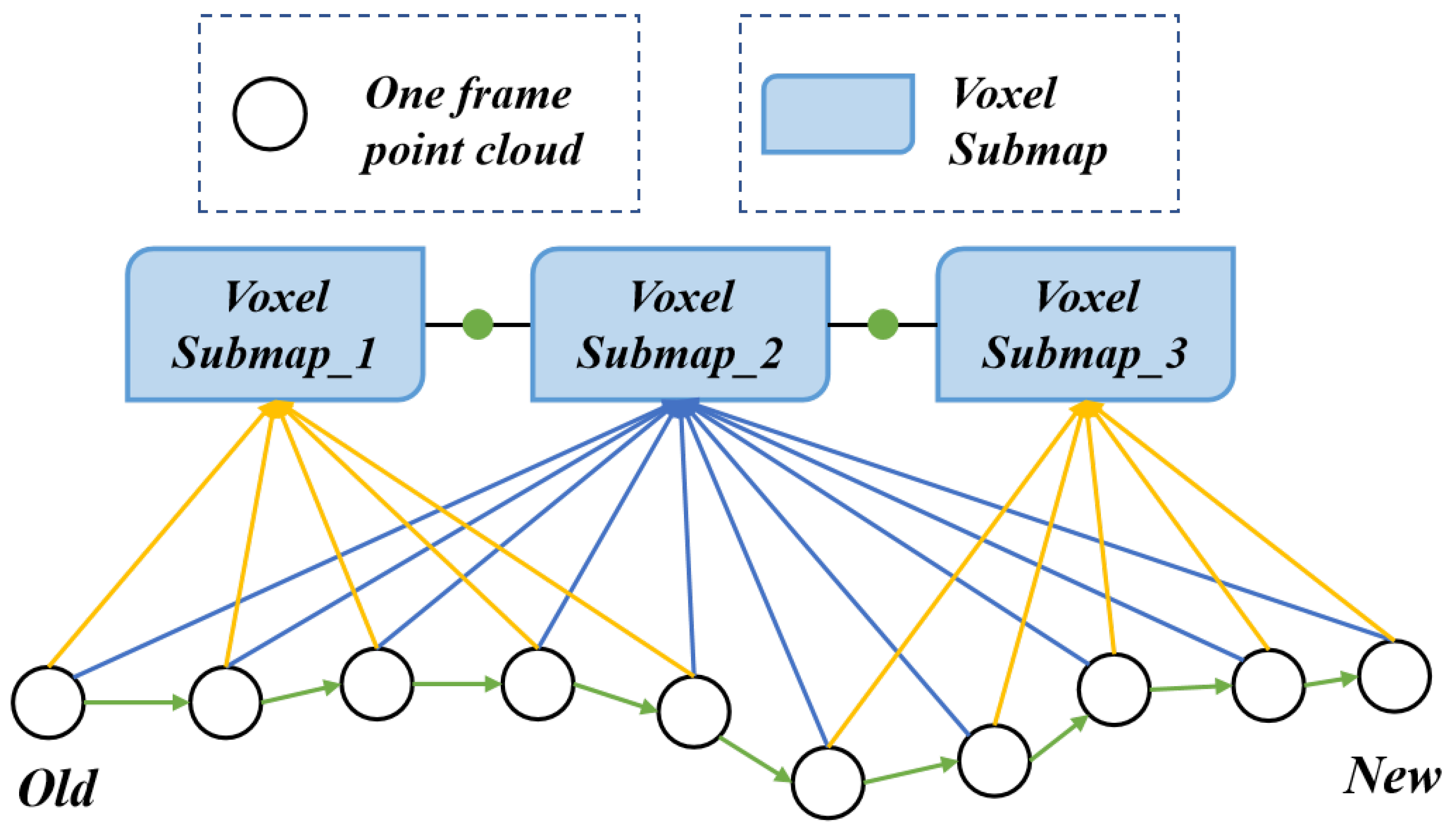
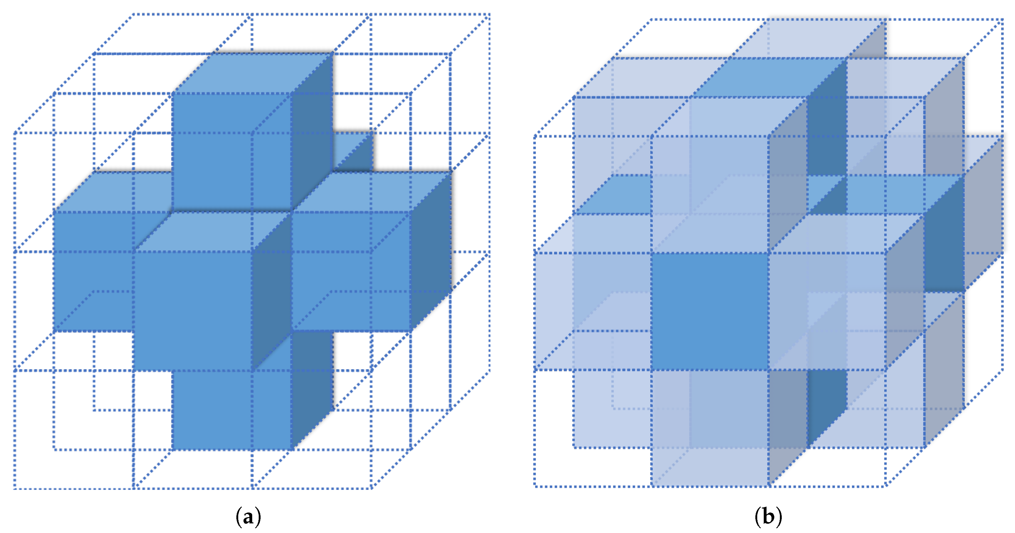
3.1.2. Surfel Feature Updating and Map Maintenance

Maps are often managed by dividing the environment into grid maps, which facilitates efficient representation and processing. Cartographer employs probabilistic grid maps for 2D indoor scenarios, while its 3D extension uses TSDFs [32]. However, continuous voxel grids are highly memory-intensive and computationally inefficient, posing significant challenges for large-scale 3D mapping applications.

To alleviate this issue, large-scale outdoor 3D mapping often divides the environment into discrete voxel units, with point cloud data stored in each voxel. This voxel-based structure significantly improves the efficiency of nearest-neighbor search, thereby enabling real-time point cloud registration and making it suitable for scalable applications.

Nevertheless, point clouds are inherently sparse compared to dense voxel grids, resulting in a large number of empty voxels marked as free space, leading to substantial memory waste. To mitigate this, we propose a hash-based voxelization scheme, as illustrated in Figure 3. A hash function maps each voxel in 3D space to a unique index, and only voxels containing point cloud data are stored in the hash table. This approach maintains the efficiency of voxel-based mapping while significantly reducing memory consumption, as it avoids allocating memory for empty or unused regions. We define the hash function $\mathit{H}(\mathit{x},\mathit{y},\mathit{z})$ to compute the hash index [33] for each voxel, as shown in Equation (3).

$$H(x,y,z)=(x·p_1+y·p_2+z·p_3)modN$$

(3)

where $(x,y,z)$ are the voxel coordinates; $p_1,p_2,p_3$ are three large prime numbers (e.g., 73856093, 193499669, 83492792); and N is the size of the hash table. We handle collisions by organizing the hash table into uniform hash buckets; each bucket stores multiple hash items, but each hash item corresponds to a unique hash value.

For efficient point cloud storage, we introduce two types of hash voxels: surfel voxels and common voxels. The former stores surfel features, which are extracted when the number of points in a voxel exceeds a predefined threshold, and these points can be well approximated by a plane. In such cases, only the surfel features are retained, while the raw point data within the voxel is discarded. This strategy enhances subsequent matching efficiency by eliminating redundant surfel fitting operations.

Each surfel voxel maintains the following attributes: the number of points m, the covariance matrix $\mathit{A}$, the surfel center $\overline{\mathit{p}}$, the normal vector $\mathit{n}$, and the planarity metric $\alpha$. When a new point cloud frame is inserted, each 3D point contributes to updating the attributes of the voxel it falls into. As a result, multiple voxels are updated in parallel, and their corresponding surfels are incrementally refined according to Equation (4), following the method proposed in [34]. Each voxel maintains at most one surfel, where the normal vector $\mathit{n}$ is computed as the eigenvector corresponding to the smallest eigenvalue ${\lambda }_3$ of the covariance matrix $\mathit{A}$.

$$\begin{array}{cc}\hfill {\overline{\mathit{p}}}_{new}& ={\displaystyle \frac{m·\overline{\mathit{p}}+{\sum }_{i=1}^N{\mathit{p}}_i}{m+N}}\hfill \\ \hfill {\mathit{A}}_{new}& ={\displaystyle \frac{m}{m+N}}\left(\mathit{A}+\overline{\mathit{p}}{\overline{\mathit{p}}}^T\right)+{\displaystyle \frac{1}{m+N}}\sum _{i=1}^N{\mathit{p}}_i{\mathit{p}}_i^T-{\overline{\mathit{p}}}_{new}{\overline{\mathit{p}}}_{new}^T\hfill \\ \hfill {\alpha }_{new}& ={\displaystyle \frac{{\lambda }_2-{\lambda }_1}{{\lambda }_1+{\lambda }_2+{\lambda }_3}}\hfill \end{array}$$

(4)

where ${\lambda }_1,{\lambda }_2,{\lambda }_3$ are the eigenvalues of ${\mathit{A}}_{new}$, and N is the number of newly inserted points.

The second class is common voxels, which is also the default type used for voxel initialization. If the number of points within a voxel exceeds the threshold but does not satisfy the planarity criterion, the voxel directly stores the point cloud. To prevent overly dense storage, a voxel-level filtering mechanism is employed to maintain a manageable point density.

As shown in Figure 4, a point cloud frame is simultaneously inserted into two neighboring voxel submaps, ensuring a 50% overlap between adjacent submaps. A new local submap is added every 80 m, and the point cloud from the latest frame is matched with the penultimate submap in the time series before being inserted into the last two submaps. The relative motion between the poses ${\mathit{T}}_1=({\mathit{R}}_1,{\mathit{t}}_1)$ and ${\mathit{T}}_2=({\mathit{R}}_2,{\mathit{t}}_2)$ for two consecutive frames is expressed by Equation (5).

$$\begin{array}{cc}\hfill \Delta \mathit{R}& =Log\left({\mathit{R}}_2^T{\mathit{R}}_1\right)\hfill \\ \hfill \Delta \mathit{t}& ={\mathit{t}}_2-{\mathit{t}}_1\hfill \end{array}$$

(5)

3.2. Real-Time Pose Estimation

We adopt a tightly coupled LiDAR-IMU fusion strategy for multi-sensor fusion. After performing IMU pre-integration, each distorted LiDAR scan is corrected to a unified time reference. The motion-compensated point cloud is then matched with the surfel features to provide geometric constraints, while the state increments obtained from IMU integration act as inertial constraints. These constraints are weighted according to their respective confidences and jointly optimized in a nonlinear framework to yield the best estimate of the system state.

For the rotation matrix $\mathit{R}$ in the $\mathit{SO}\left(3\right)$ manifold and its corresponding tangent space vector $\mathit{r}$, we define the operations ⊕ and ⊖. These operations are mathematically expressed in Equation (6).

$$\begin{array}{cc}\hfill \mathit{R}\oplus \mathit{r}& =\mathit{R}\mathrm{Exp}\left(\mathit{r}\right)\in SO\left(3\right)\hfill \\ \hfill {\mathit{R}}_1\ominus {\mathit{R}}_2& =\mathrm{Log}\left({\mathit{R}}_2^T{\mathit{R}}_1\right)\in \mathfrak{so}\left(3\right)\hfill \end{array}$$

(6)

The raw acceleration and angular velocity data measured by the IMU are expressed in the IMU coordinate system ${\left(·\right)}^b$ at time t, as shown in Equation (7).

$$\begin{array}{cc}\hfill {\tilde{\mathit{\omega }}}^b\left(t\right)& ={\mathit{\omega }}^b\left(t\right)+{\mathit{b}}_g\left(t\right)+{\mathit{\eta }}_g\left(t\right)\hfill \\ \hfill {\tilde{\mathit{a}}}^b\left(t\right)& ={\mathit{R}}_b^{w\mathsf{T}}\left({\mathit{a}}_b^w-{\mathit{g}}^w\right)+{\mathit{b}}_a\left(t\right)+{\mathit{\eta }}_a\left(t\right)\hfill \end{array}$$

(7)

where ${\mathit{\eta }}_g$ and ${\mathit{\eta }}_a$ represent the Gaussian noise of the gyroscope and accelerometer, respectively, and ${\mathit{b}}_g$ and ${\mathit{b}}_a$ represent the bias of the gyroscope and accelerometer. After obtaining the IMU measurements, the first integral of ${\mathit{\omega }}^b\left(t\right)$ and the second integral of ${\mathit{a}}_b^w$ are used to derive the IMU integration constraints.

Since the bias of gyroscope and accelerometer is time-varying and accumulates over time, it progressively degrades the accuracy of the estimated acceleration and angular velocity. To mitigate this effect, we estimate the bias using a tightly coupled approach. The corresponding state model is defined in Equations (8) and (9).

$$\mathit{x}\doteq \left[\begin{array}{cccccc}{\mathit{R}}_b^w& {\mathit{p}}_b^w& {\mathit{v}}_b^w& {\mathit{b}}_g& {\mathit{b}}_a& {\mathit{g}}^w\end{array}\right]\in \mathcal{M}$$

(8)

$$\begin{array}{cc}\hfill {\mathit{x}}_1\ominus {\mathit{x}}_2& =\left[\begin{array}{cccccc}\mathrm{Log}\left({\mathit{R}}_2^{\mathsf{T}}{\mathit{R}}_1\right)& {\mathit{p}}_1-{\mathit{p}}_2& {\mathit{v}}_1-{\mathit{v}}_2& {\mathit{b}}_{g1}-{\mathit{b}}_{g2}& {\mathit{b}}_{a1}-{\mathit{b}}_{a2}& {\mathit{g}}_1-{\mathit{g}}_2\end{array}\right]\hfill \\ \hfill & =\left[\begin{array}{cccccc}\delta \mathit{\theta }& \delta \mathit{p}& \delta \mathit{v}& \delta {\mathit{b}}_g& \delta {\mathit{b}}_a& \delta {\mathit{g}}^w\end{array}\right]\hfill \\ \hfill & =\delta \mathit{x}\hfill \\ \hfill \mathit{x}\oplus \delta \mathit{x}& =\left[\begin{array}{cccccc}\mathit{x}\mathrm{Exp}\left(\delta \mathit{\theta }\right)& \mathit{p}+\delta \mathit{p}& \mathit{v}+\delta \mathit{v}& {\mathit{b}}_g+\delta {\mathit{b}}_g& {\mathit{b}}_a+\delta {\mathit{b}}_a& {\mathit{g}}^w+\delta {\mathit{g}}^w\end{array}\right]\hfill \end{array}$$

(9)

The rotation matrix $\mathit{R}$ lies on the Lie group $\mathit{SO}\left(\mathit{3}\right)$, and the whole system state $\mathit{x}$ is defined on a product manifold $\mathcal{M}$. To ensure correct updates in this nonlinear state space, we adopt a manifold-based optimization strategy.

The operations ⊕ and ⊖ are introduced to map between the manifold and its tangent space, enabling the definition of residuals and state updates in a geometrically consistent manner. This formulation is significant for achieving stable and accurate estimation in our tightly coupled LiDAR-IMU fusion framework.

We preprocess the point cloud data using the a priori pose derived from IMU integration to compensate for motion distortion. Additionally, point cloud matching with surfel features serves as one constraint, while the relative state obtained from IMU integration provides another constraint.

These constraints are then weighted by their respective covariance matrices, forming a nonlinear optimization problem. The optimal estimation of the system’s state variables is ultimately obtained through iterative solving.

The newly obtained point cloud ${\mathit{p}}_l$ is transformed into the world coordinate system as ${\mathit{p}}_w$ using the initial pose prediction, which serves as the initial mapping position of ${\mathit{p}}_l$. For each point in the world, we determine its corresponding voxel using the hash function defined in Equation (3). Within that voxel and its 18 spatially nearest neighbors in continuous space, as illustrated in Figure 5, we search for the nearest surfel voxel and the closest point within a common voxel.

If the surfel feature in the surfel voxel is closer to the nearest point in the common voxel than the nearest point in the common voxel to ${\mathit{p}}_w$, then ${\mathit{p}}_l$ is matched with the surfel feature in the surfel voxel. Otherwise, if a point in a common voxel is closer to ${\mathit{p}}_w$, we look up the point in that common voxel and its 18 spatially nearest neighboring voxels. As shown in Equations (1) and (2), plane fitting is performed using five points from the common voxel.

If a point ${\mathit{p}}_i^{l_k}$ lies precisely on the surfel, then after the pose transformation ${\mathit{T}}_{l_k}^w$, the point-to-surfel distance is expected to converge to zero as optimization proceeds. Consequently, the estimation of the carrier pose transformation can be formulated as a least-squares optimization problem that minimizes the sum of squared point-to-plane distances, as defined in Equation (10).

$$\mathit{e}=\sum _{i=1}^N{\left({({\mathit{R}}_{l_k}^w{\mathit{p}}_i^{l_k}+{\mathit{t}}_{l_k}^w-{\overline{\mathit{p}}}_i)}^T·{\mathit{n}}_i\right)}^2$$

(10)

With the Jacobian matrix $\mathit{H}$ in Equation (11), we can linearize the point-to-plane distance constraint.

$$\mathit{H}={\mathit{n}}^{\top }\left[\begin{array}{ccc}-{\mathit{R}}_{{\mathit{b}}_j}^w{\left({\mathit{R}}_l^b{\mathit{p}}_j^{l_j}+{\mathit{p}}_l^b\right)}^{\wedge }& {\mathit{I}}_{3\times 3}& {\mathbf{0}}_{3\times 12}\end{array}\right],\mathit{H}\in {\mathbb{R}}^{1\times 18}$$

(11)

This constraint is omitted from the objective function in Equation (10) if the distance between a point and its nearest surfel feature in the corresponding hash voxel exceeds a predefined threshold or if the associated planarity falls below a specified threshold.

For the optimization problem defined in Equation (10), each iteration requires transforming the LiDAR points from the sensor frame to the world frame using the updated pose estimate, followed by re-identifying the nearest surfel based on spatial proximity. This repeated surfel association process incurs significant computational overhead.

To address this issue, we propose a surfel matching strategy in which surfel associations are performed only once during the first iteration. The associated surfel features for each valid matched point are cached and reused in subsequent iterations, thereby avoiding redundant computations and accelerating the overall optimization process. The detailed point cloud matching algorithm based on memoized surfel retrieval is provided in Appendix B.

The process of integrating IMU data using Equation (12). The position, velocity and orientation at time step j are calculated as follows, where ${\mathit{p}}_j$ and ${\mathit{v}}_j$ are the position and velocity at time j, ${\mathit{R}}_j$ is the rotation matrix, and ${\tilde{\mathit{a}}}_k$, ${\mathit{b}}_{a_k}$, and ${\mathit{\eta }}_{a_k}$ represent the measured accelerations, accelerometer biases, and accelerometer noise, respectively:

$$\begin{array}{cc}\hfill {\mathit{p}}_j& ={\mathit{p}}_i+\sum _{k=i}^{j-1}\left[{\mathit{v}}_k\Delta t+{\displaystyle \frac{1}{2}}\mathit{g}\Delta t^2+{\displaystyle \frac{1}{2}}{\mathit{R}}_k({\tilde{\mathit{a}}}_k-{\mathit{b}}_{a_k}-{\mathit{\eta }}_{a_k})\Delta t^2\right]\hfill \\ \hfill {\mathit{v}}_j& ={\mathit{v}}_i+\mathit{g}\Delta t_{ij}+\sum _{k=i}^{j-1}\left[{\mathit{R}}_k({\tilde{\mathit{a}}}_k-{\mathit{b}}_{a_k}-{\mathit{\eta }}_{a_k})\Delta t\right]\hfill \\ \hfill {\mathit{R}}_j& ={\mathit{R}}_i\prod _{k=1}^{j-1}\mathrm{Exp}\left(({\tilde{\mathit{\omega }}}_k-{\mathit{b}}_{{\omega }_k}-{\mathit{\eta }}_{g_k})\Delta t\right)\hfill \end{array}$$

(12)

The propagation of uncertainty throughout this process is described in Equation (13).

$${\check{\mathit{P}}}_{i+1}={\mathit{F}}_{\delta \mathit{x}}{\check{\mathit{P}}}_i{\mathit{F}}_{\delta \mathit{x}}^{\top }+{\mathit{F}}_{{\mathit{\eta }}_i}\mathit{Q}{\mathit{F}}_{{\mathit{\eta }}_i}^{\top },{\check{\mathit{P}}}_0={\widehat{\mathit{P}}}_{k-1}$$

(13)

The matrices involved in this propagation are defined in Equations (14) and (15):

$${\mathit{F}}_{\delta \mathit{x}}=\left[\begin{array}{cccccc}\mathrm{Exp}(-{\check{\mathit{\omega }}}_i)\Delta t& \mathbf{0}& \mathbf{0}& -{\mathit{J}}_r({\check{\mathit{\omega }}}_i\Delta t)\Delta t& \mathbf{0}& \mathbf{0}\\ -{\displaystyle \frac{1}{2}}{\check{\mathit{R}}}_{b_i}^w{\left({\check{\mathit{a}}}_i\right)}^{\wedge }\Delta t^2& \mathit{I}& \mathit{I}\Delta t& \mathbf{0}& -{\displaystyle \frac{1}{2}}{\check{\mathit{R}}}_{b_i}^w\Delta t^2& \mathbf{0}\\ -{\check{\mathit{R}}}_{b_i}^w{\left({\check{\mathit{a}}}_i\right)}^{\wedge }\Delta t& \mathbf{0}& \mathit{I}& \mathbf{0}& -{\check{\mathit{R}}}_{b_i}^w\Delta t& \mathbf{0}\\ \mathbf{0}& \mathbf{0}& \mathbf{0}& \mathit{I}& \mathbf{0}& \mathbf{0}\\ \mathbf{0}& \mathbf{0}& \mathbf{0}& \mathbf{0}& \mathit{I}& \mathbf{0}\\ \mathbf{0}& \mathbf{0}& \mathbf{0}& \mathbf{0}& \mathbf{0}& \mathit{I}\end{array}\right]$$

(14)

$${\mathit{F}}_{{\mathit{\eta }}_i}=\left[\begin{array}{cccc}-{\mathit{J}}_r({\check{\mathit{\omega }}}_i\Delta t)\Delta t& \mathbf{0}& \mathbf{0}& \mathbf{0}\\ \mathbf{0}& -{\displaystyle \frac{1}{2}}{\check{\mathit{R}}}_{b_i}^w\Delta t^2& \mathbf{0}& \mathbf{0}\\ \mathbf{0}& -{\check{\mathit{R}}}_{b_i}^w\Delta t& \mathbf{0}& \mathbf{0}\\ \mathbf{0}& \mathbf{0}& \mathit{I}\Delta t& \mathbf{0}\\ \mathbf{0}& \mathbf{0}& \mathbf{0}& \mathit{I}\Delta t\\ \mathbf{0}& \mathbf{0}& \mathbf{0}& \mathbf{0}\end{array}\right]$$

(15)

Based on these foundations, a nonlinear optimization problem is constructed to combine LiDAR and IMU data, as shown in Equation (16).

$$\begin{array}{cc}\hfill \mathit{x}& =arg\underset{\mathit{x}}{min}\left({∥{\mathit{x}}_k\ominus {\check{\mathit{x}}}_k∥}_{{\check{\mathit{P}}}_k^{-1}}^2+\sum _{j=1}^n{∥{\mathit{h}}_j\left({\mathit{x}}_k\right)∥}_{{\mathit{Q}}_j^{-1}}^2\right)\hfill \end{array}$$

(16)

where ${\mathit{x}}_k$ denotes the system state variables, ${\check{\mathit{x}}}_k$ represents the state estimates obtained from IMU integration, and ${\mathit{P}}_k$ and ${\mathit{Q}}_j$ denote the covariances associated with IMU integration and point cloud alignment, respectively. The weighting matrix ${\mathit{Q}}_j$ is positively correlated with the planarity metric $\alpha$.

By linearizing the nonlinear optimization problem described in Equation (16), we derive its linearized least-squares form, as shown in Equation (17). The Gauss-–Newton method is then employed to solve for the perturbation $\delta \mathit{x}$ in the manifold space.

$$\begin{array}{cc}\hfill \delta \mathit{x}& =arg\underset{\delta \mathit{x}}{min}\left({∥{\mathit{x}}_k\ominus {\check{\mathit{x}}}_k\oplus \mathit{J}\left({\mathit{x}}_k\right)\delta {\mathit{x}}_k∥}_{{\mathit{P}}_k^{-1}}^2+\sum _{j=1}^N{∥{\mathit{d}}_j+{\mathit{H}}_j\delta \mathit{x}∥}_{{\mathit{Q}}_j^{-1}}^2\right)\hfill \\ \hfill & =\left(-\mathit{K}{\mathit{d}}_k-(\mathit{I}-\mathit{K}\mathit{H})\mathit{J}{\left({\mathit{x}}_k\right)}^{-1}({\mathit{x}}_k^i\ominus {\check{\mathit{x}}}_k)\right)\hfill \end{array}$$

(17)

where ${\mathit{H}}_j$ is defined in Equation (11). Based on the solution to Equation (17), the system state ${\mathit{x}}_k$ and the covariance matrix ${\mathit{P}}_k$ are updated iteratively according to Equation (18).

$$\begin{array}{cc}\hfill {\mathit{x}}_{k+1}& ={\mathit{x}}_k+\delta \mathit{x}\hfill \\ \hfill {\mathit{P}}_{k+1}& =E\left(\delta \mathit{x}\delta {\mathit{x}}^{\top }\right)\hfill \\ \hfill & ={\mathit{J}}^{-1}{\mathit{P}}_k{\mathit{J}}^{-\top }-\mathit{K}\mathit{H}{\mathit{J}}^{-1}{\mathit{P}}_k{\mathit{J}}^{-\top }\hfill \end{array}$$

(18)

where $\mathit{E}$ denotes the mathematical expectation. A complete derivation of Equations (17) and (18) is provided in Appendix A for reference.

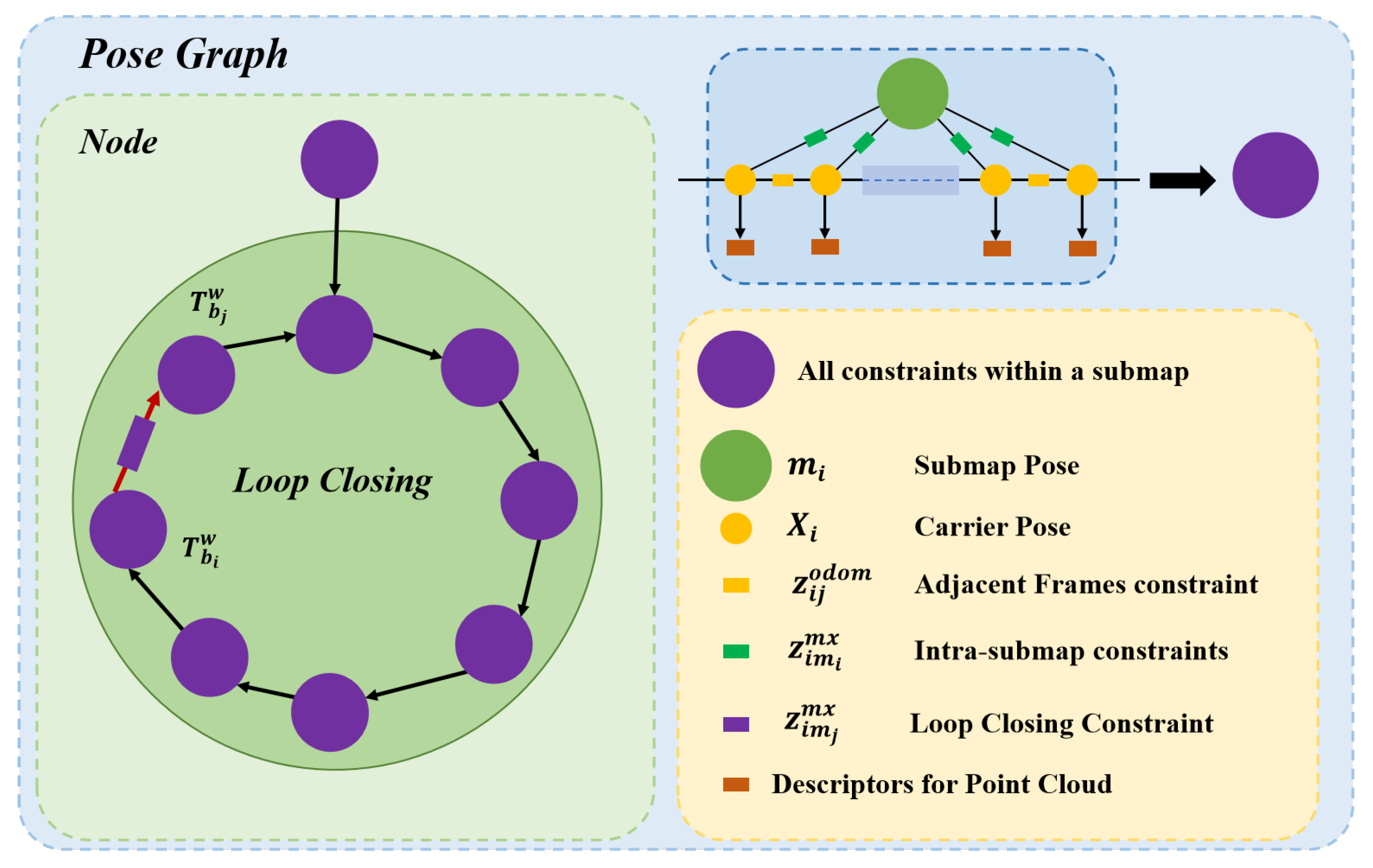
3.3. Loop Closing and Global Optimization

We adopt the descriptor proposed in Link3D [35] for loop closure detection. The global optimization process incorporates both intra-submap constraint residuals and loop closure residuals. A pose graph is constructed to perform global optimization, as illustrated in Figure 6.

The intra-submap constraints serve to enforce the relative poses among all LiDAR nodes within the same submap. These relative poses are defined with respect to the origin of the corresponding voxel submap.

The pose of its origin represents the pose of a voxel submap. In the LiDAR-inertial odometry module, the transformation matrix of the LiDAR node ${\mathit{X}}_i$, originally denoted as ${\mathit{T}}_i^w$, is simplified as ${\mathit{T}}_i^w$ for convenience. Similarly, the transformation matrix of voxel submap ${\mathit{M}}_j$, denoted as ${\mathit{T}}_{M_j}^w$, is simplified as ${\mathit{T}}_j^w$.

The relative transformation between a LiDAR node and its corresponding voxel submap in the world coordinate system is denoted as ${\mathit{h}}_{ij}$ and defined in Equation (19):

$$\begin{array}{cc}\hfill {\mathit{h}}_{ij}& =({\mathit{R}}_{ij},{\mathit{t}}_{ij})={\left({\mathit{T}}_i^w\right)}^{-1}·{\mathit{T}}_j^w\hfill \\ \hfill & =\left[\begin{array}{cc}{\mathit{R}}_i^{w\top }{\mathit{R}}_j^w& {\mathit{R}}_i^{w\top }({\mathit{t}}_j^w-{\mathit{t}}_i^w)\\ \mathbf{0}& 1\end{array}\right]\hfill \end{array}$$

(19)

Let ${\mathit{T}}_i$ and ${\mathit{T}}_j$ denote the global poses of the LiDAR node ${\mathit{X}}_i$ and the voxel submap ${\mathit{M}}_j$, respectively. The residual constructed from intra-submap constraints is given by Equation (20).

$$\begin{array}{cc}\hfill {\mathit{e}}_{\mathrm{intra}}& =\mathrm{Log}\left({\mathit{h}}_{ij}^{-1}{\mathit{T}}_i^{-1}{\mathit{T}}_j\right)\hfill \\ \hfill & =\left[\begin{array}{cc}\mathrm{Log}\left({\mathit{R}}_{ij}^{\top }{\mathit{R}}_i^{\top }{\mathit{R}}_j\right)& {\mathit{R}}_{ij}^{\top }{\mathit{R}}_i^{\top }({\mathit{t}}_j-{\mathit{t}}_i)-{\mathit{R}}_{ij}^{\top }{\mathit{t}}_{ij}\\ \mathbf{0}& 1\end{array}\right]\hfill \end{array}$$

(20)

4. Experiment and Discussion

To validate the effectiveness of our proposed algorithms, we conduct extensive experiments on both publicly available datasets and our self-built mobile robot platforms. The evaluation focuses on pose estimation accuracy, loop closure, map consistency, generalization across different robot platforms, and real-time performance. We compare our methods with those of mainstream algorithms, such as Faster-LIO, Fast-LOAM, and LIO-SAM. Among them, VOX-LIOM incorporates loop closure detection and global pose graph optimization.

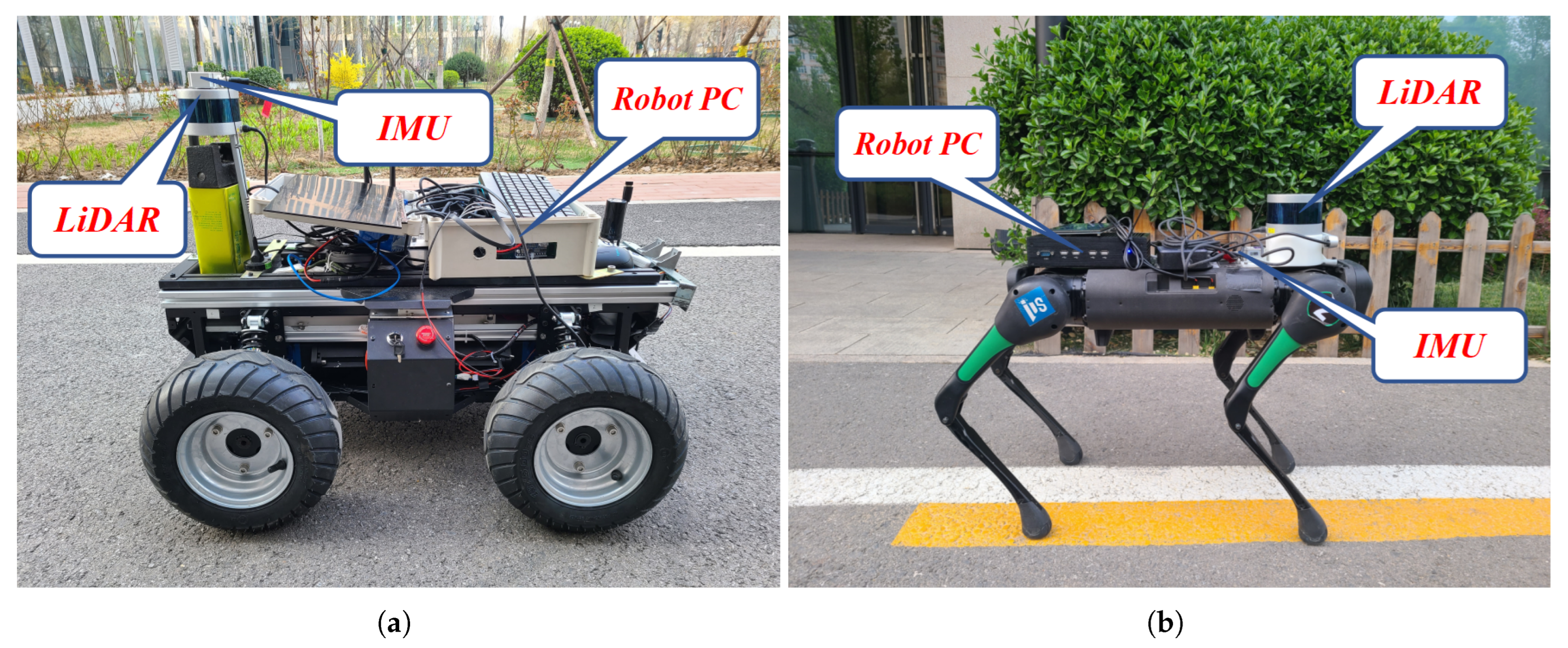
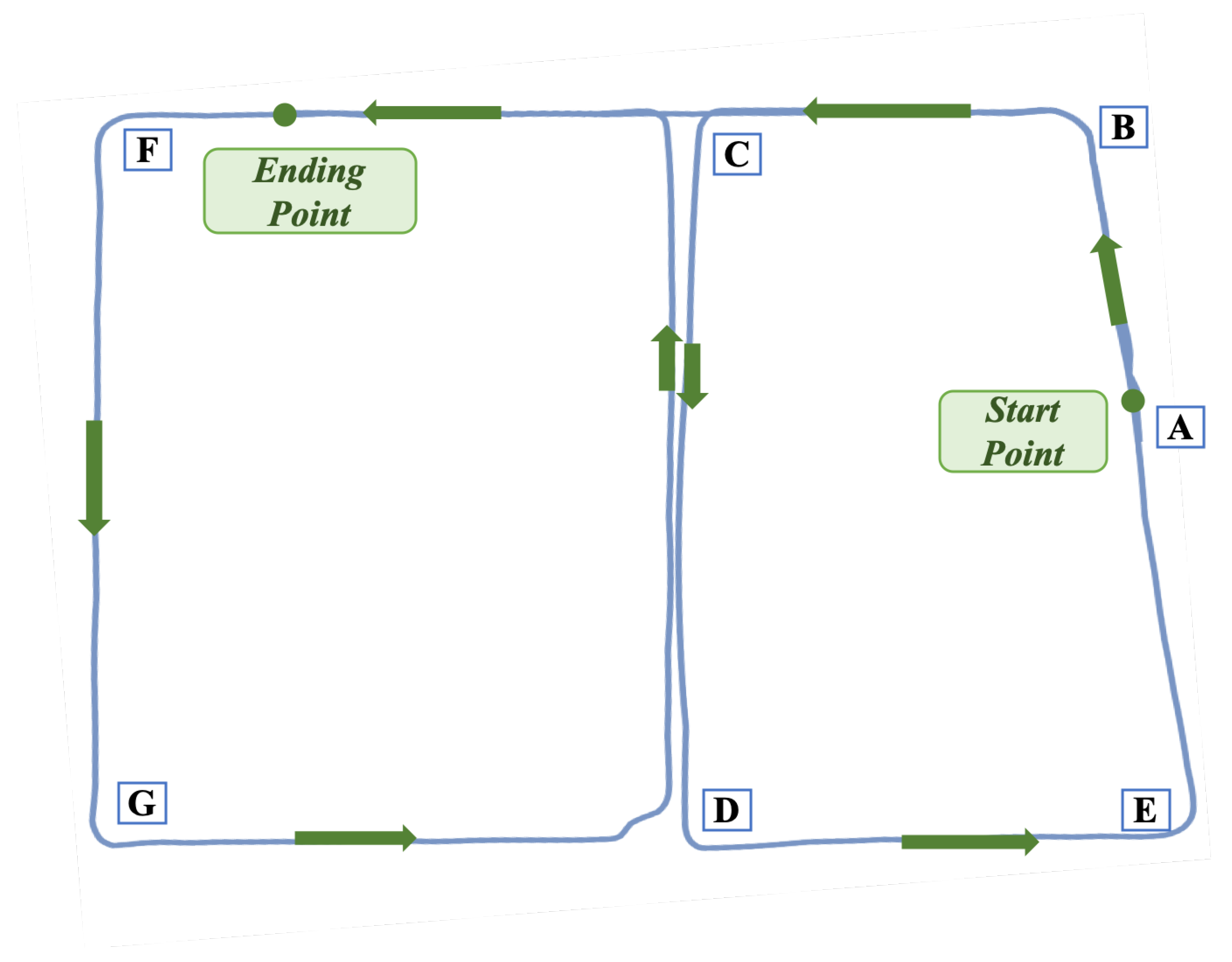
4.1. Experimental Design and Platforms

The KITTI dataset [36] is among the most widely used public benchmarks for evaluating pose estimation and mapping in autonomous driving. It provides high-quality sensor data, including LiDAR, cameras, and GPS, with accurate calibration and precise time synchronization. Among its sequences, 00 and 05 are the most representative and frequently used. We conduct a series of experiments on these two sequences to evaluate the accuracy of pose estimation, the performance of global optimization, and the overall consistency of our map.

The NCLT dataset [37] is particularly suitable for evaluating the long-term performance of LiDAR-inertial SLAM algorithms due to its extended trajectory lengths, large-scale environments, and high-quality sensor data. The datasets were collected across different seasons and under varying weather conditions throughout the year. We conduct experiments on sequences 01 and 02 to validate the accuracy of pose estimation, real-time performance, and mapping effectiveness. The key characteristics of these sequences are summarized in

Table 1. Key Properties of the KITTI and NCLT Datasets Utilized in Our Experiments.

Seq.	Capture Time	Duration (s)	Point Cloud Frames	Trajectory Length (m)	Weather	Snowy
kitti_00	3 October 2011	470	4544	3700	Partly cloudy	No
kitti_05	30 September 2011	270	2762	2200	Cloudy	No
nclt_01	10 January 2013	1025	7775	1100	Overcast	Yes
nclt_02	29 April 2012	2600	25,819	3100	Sunny	No

.

In general, obtaining ground truth pose data for self-built mobile robot platforms requires expensive RTK equipment, making it impractical for large-scale experiments. Therefore, quantitative evaluations of pose estimation accuracy are conducted using publicly available datasets with ground truth. For our self-built mobile robot platforms, as shown in Figure 7, we focus on evaluating the algorithm’s generalizability across different platforms and its mapping performance in real-world scenarios.

The four-wheeled mobile robot is capable of performing tasks such as autonomous goods delivery in campus environments, where the accuracy and stability of localization and mapping directly affect operational reliability. The quadruped robot, designed for autonomous inspection, also demands high-precision localization and mapping, particularly in complex campus settings. Unlike the four-wheeled platform, the legged structure of the quadruped robot introduces more pronounced motion disturbances during locomotion.

In comparison, the four-wheeled platform offers smoother movement, making it better suited for long-term mapping in larger environments. Conversely, the quadruped robot presents a more challenging scenario due to its dynamic and uneven motion characteristics.

Both robotic platforms are equipped with identical sensors and computing hardware. Each platform utilizes a 16-beam mechanical Velodyne VLP-16 LiDAR and a MEMS-based LPMS-IG1 inertial measurement unit (IMU). A detailed summary of the datasets collected by these platforms is provided in

Table 2. Main Information of Self-built Mobile Robots.

Platform	Duration (s)	Frames	Length (m)	Characteristics
Four-Wheeled	1611	15,980	1050	Steady
Quadruped	295	2926	267	Bumps

. The dataset names shown in the table are used consistently throughout this paper to represent the corresponding datasets. All experiments were conducted at the Beijing Institute of Technology (BIT).

To evaluate the runtime performance of the proposed algorithm on mobile robotic platforms, our experiments were conducted using a computing unit equipped with an Intel i7-6700HQ CPU and 16 GB of RAM.

4.2. Evaluation Metrics

We evaluate our algorithm in terms of localization accuracy, overall mapping quality, and computational efficiency. Specifically, localization accuracy is assessed using publicly available datasets with ground-truth trajectories. We compute the absolute pose error (APE) using the open-source evaluation tool EVO [38] and report the mean APE as the primary metric for evaluating trajectory accuracy. The APE is computed by aligning the estimated and ground-truth trajectories and includes metrics such as maximum error (Max), mean error (Mean), median error (Median), root mean square error (RMSE), and standard deviation (Std).

For overall mapping performance and loop closure evaluation, global consistency is used as the key criterion. Global consistency is used as the primary criterion for evaluating the overall mapping results and loop closing experiments, ensuring that the mapping results at the exact location are free from noticeable drift or overlapping artifacts when the robot passes through the area multiple times.

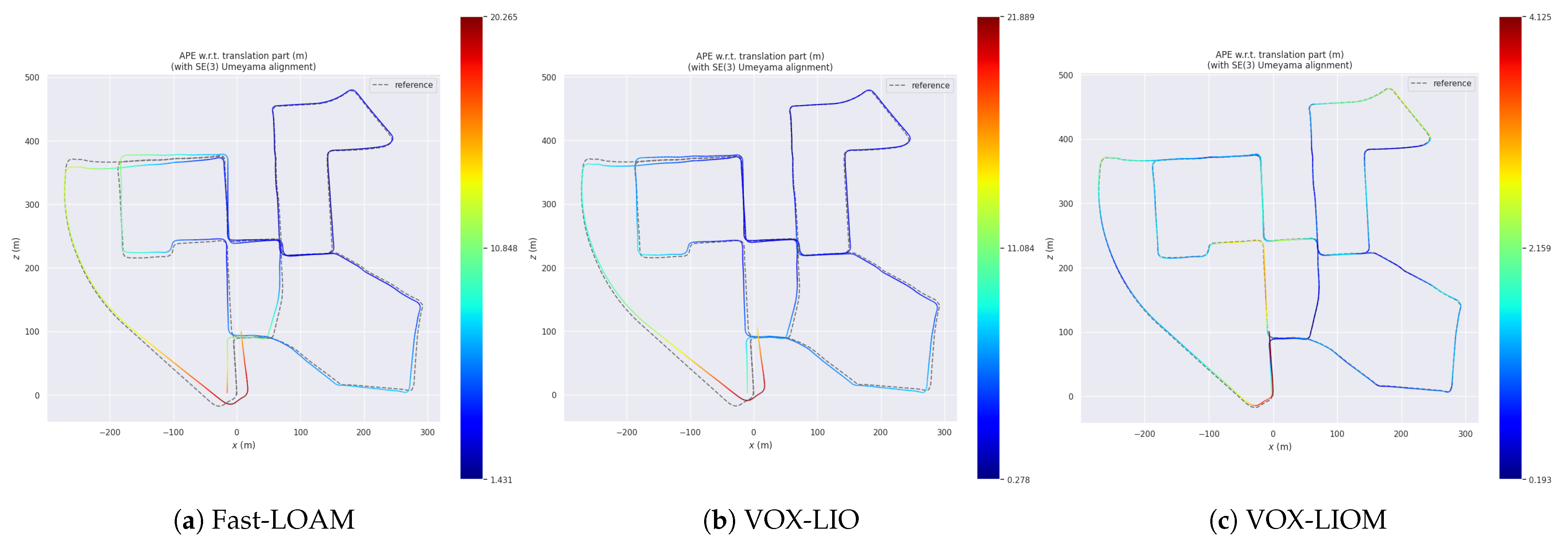
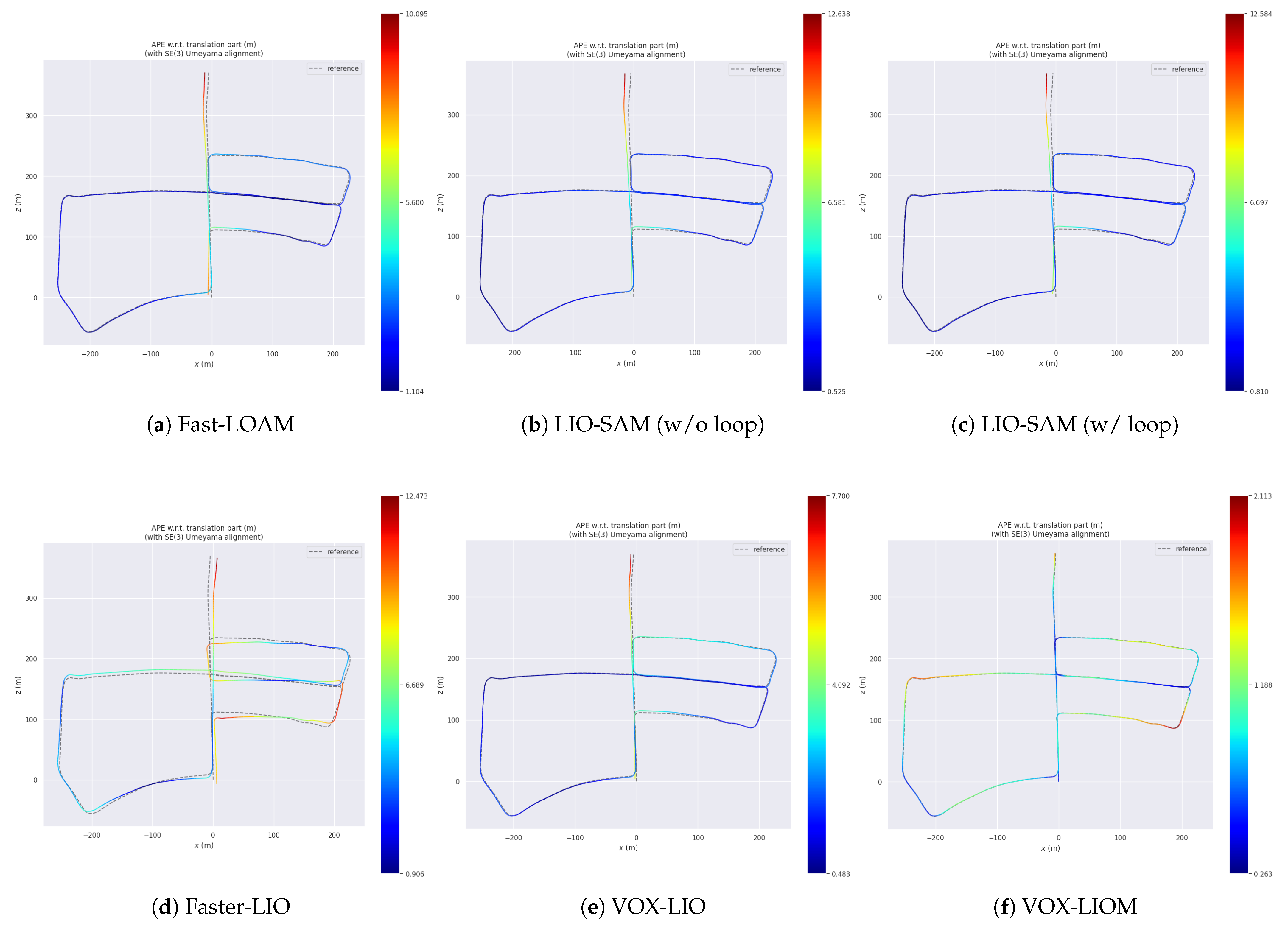
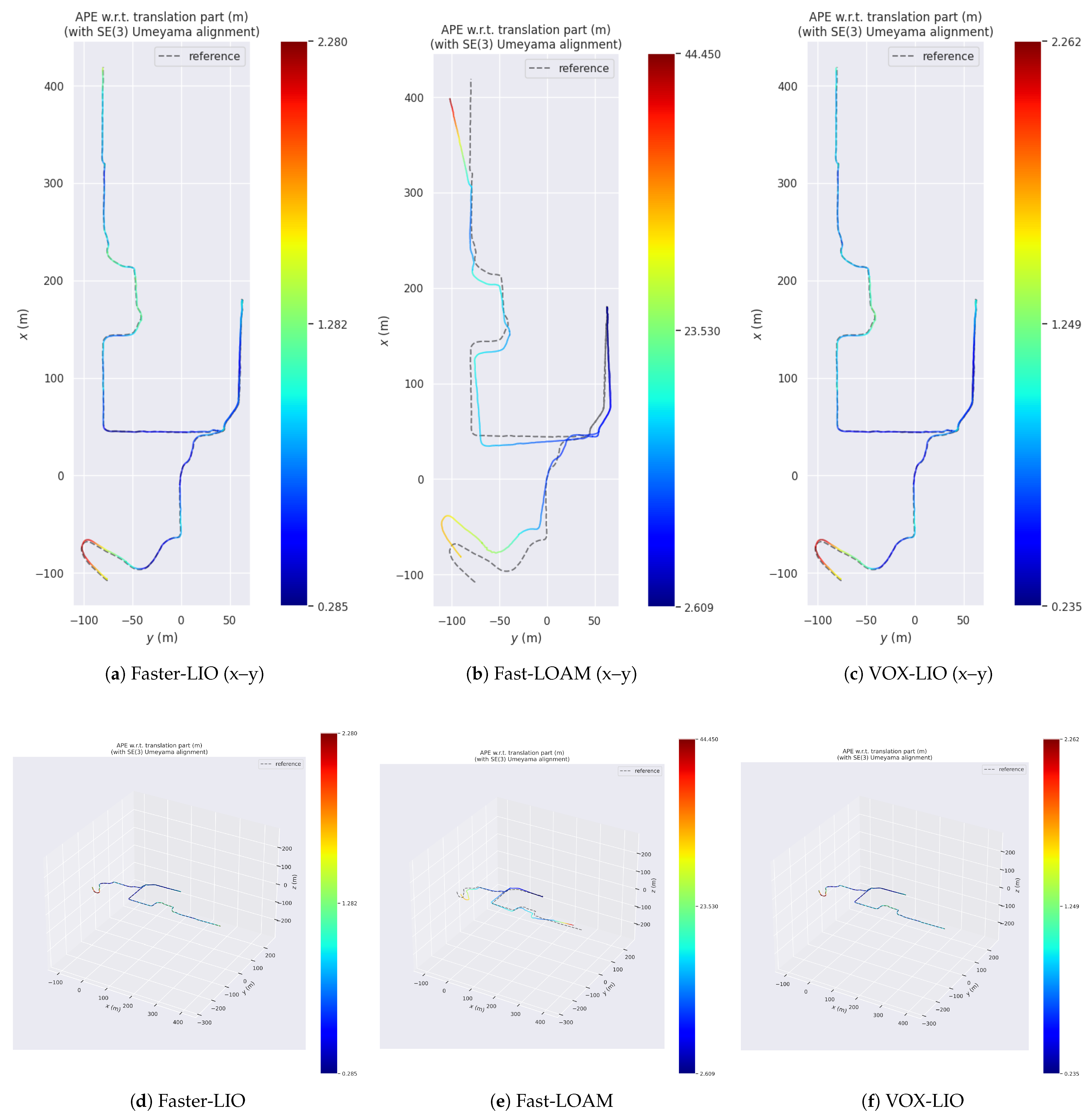
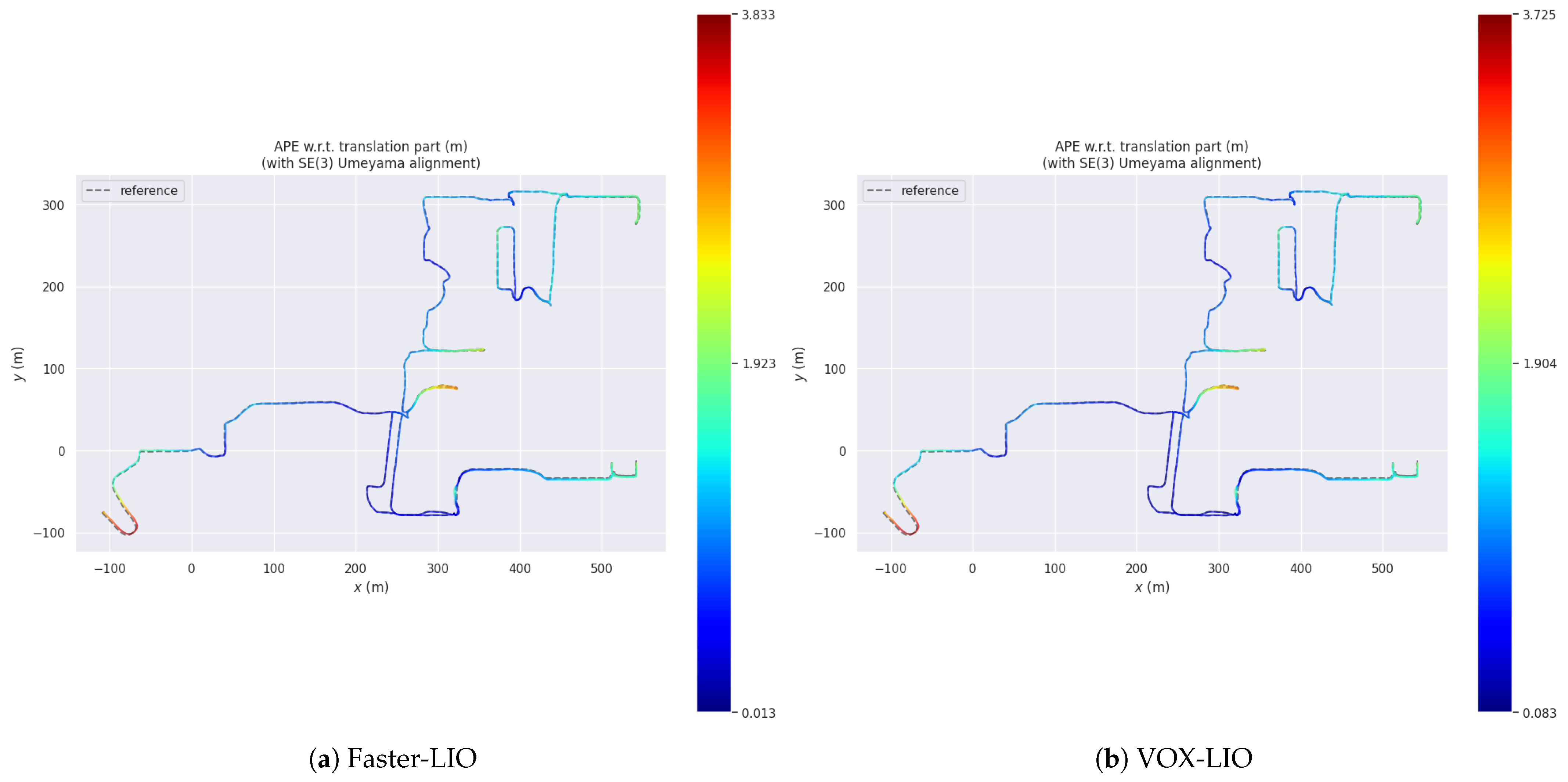
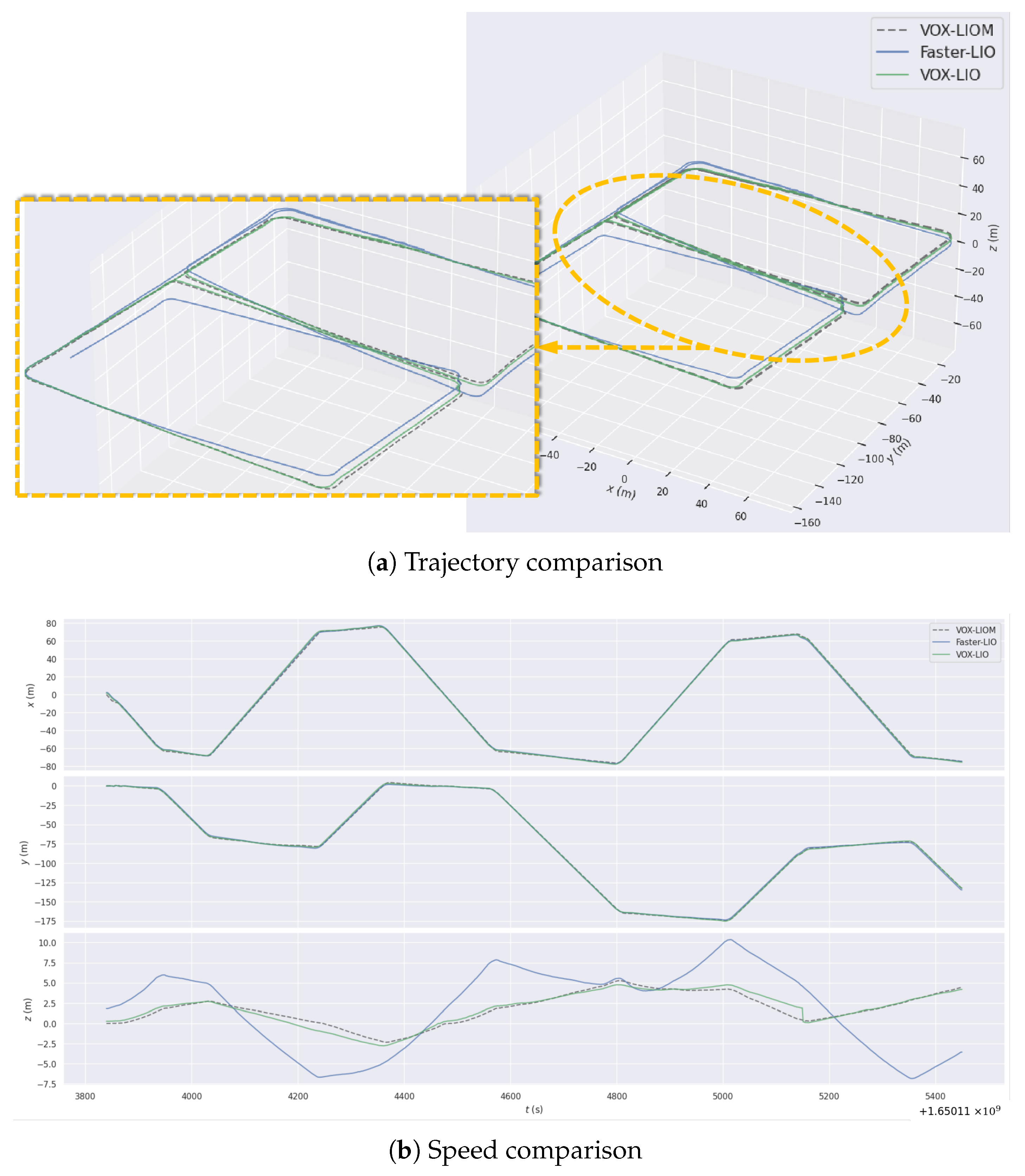
4.3. Pose Estimation Accuracy Experiment

We conducted trajectory accuracy comparison experiments using two sequences from the kitti_00 and kitti_05, which are among the longest and most representative in the benchmark. The experimental results are illustrated in Figure 8 and Figure 9, and the corresponding quantitative analysis is summarized in

Table 3. Trajectory accuracy comparison results on kitti_00, kitti_05, nclt_01, and nclt_02. The symbol × indicates system failure. Methods with a maximum error exceeding 50 m are excluded from detailed accuracy evaluation.

Seq.	Method	Max (m)	Mean (m)	Median (m)	RMSE (m)	Std (m)
kitti_00	VOX-LIO	21.74	5.59	4.56	7.10	4.37
	VOX-LIOM	4.13	1.48	1.35	1.66	0.76
	Fast-LOAM	20.27	6.87	5.56	8.18	4.45
	LIO-SAM	×	×	×	×	×
kitti_05	VOX-LIO	7.70	2.20	2.00	2.58	1.35
	VOX-LIOM	2.11	0.98	0.93	1.06	0.39
	Fast-LOAM	10.10	3.06	2.42	3.58	1.86
	Faster-LIO	12.47	6.10	5.56	6.60	2.54
	LIO-SAM (w/o loop)	12.95	4.02	3.66	4.41	1.82
	LIO-SAM (w/loop)	4.71	3.30	3.20	3.38	0.71
nclt_01	VOX-LIO	2.26	0.84	0.80	0.93	0.38
	Faster-LIO	2.28	0.89	0.83	0.96	0.38
	Fast-LOAM	44.4	15.3	14.6	17.7	8.7
	LIO-SAM	×	×	×	×	×
nclt_02	VOX-LIO	3.72	1.10	0.99	1.28	0.64
	Faster-LIO	3.83	1.15	1.04	1.32	0.66
	Fast-LOAM	×	×	×	×	×
	LIO-SAM	×	×	×	×	×

. For methods with a maximum absolute pose error (Max) exceeding 50 m, we do not consider them for a detailed accuracy evaluation.

The results in Table 3 show that VOX-LIO and VOX-LIOM achieve notable improvements in mean absolute pose error (APE) on both kitti_00 and kitti_05. Specifically, VOX-LIO reduces the mean APE by 18.6% and 28.1% compared to Fast-LOAM on kitti_00 and kitti_05, respectively. The improvement over Faster-LIO on sequence 05 is even more significant, reaching 63.9%. Building on this, VOX-LIOM further improves the estimation accuracy, achieving reductions of 78.5% and 67.7% in mean APE relative to Fast-LOAM on kitti_00 and kitti_05, respectively. Compared to Faster-LIO, VOX-LIOM reduces the mean error on kitti_05 by 83.9%.

Since LIO-SAM requires a high-frequency IMU to function correctly, this method necessitates the use of the KITTI raw dataset for evaluation. However, one problem remains unsolved: the intrinsic parameters of the IMU are unknown, which significantly affects the accuracy of LIO-SAM. As a result, LIO-SAM fails to produce reasonable results on kitti_00, where severe drift is observed due to improper IMU pre-integration caused by inaccurate intrinsic calibration.

Current mainstream SLAM algorithms, such as Fast-LOAM and Faster-LIO, typically construct constraints by fitting a plane to the five nearest neighbors (in Euclidean distance) from the map for each point in the current scan. The pose is then estimated by minimizing the point-to-plane distance. However, this approach may lead to incorrect plane fitting when the surrounding points lack sufficient geometric diversity, thereby degrading the accuracy of point cloud registration. Increasing the number of nearest neighbors to improve plane fitting stability significantly raises computational complexity and may introduce non-planar points, further compromising accuracy.

To address this issue, we propose a map management strategy based on adaptive hash voxels that enables the long-term accumulation of planar observations within each surfel voxel. This approach allows the construction of more reliable and stable surfel-based planar features by leveraging richer historical point cloud data. For Faster-LIO, a notable limitation stems from the KITTI dataset, which lacks a stationary initialization phase. Because the vehicle is already in motion at the beginning of the sequence, the gravity estimation based on stationary initialization becomes biased, leading to larger trajectory errors.

In contrast to Faster-LIO, Fast-LOAM utilizes both point-to-plane and point-to-line constraints, incorporating line features. However, the sparsity of LiDAR point clouds means that few points align with real linear structures. In practice, most “line features” are planar points near edges, better treated as planar features. Consequently, these line features are not sufficiently robust, and their inclusion in the optimization process does not necessarily improve overall registration accuracy. As a result, Fast-LOAM performs slightly worse than our proposed method.

LIO-SAM forms a loosely-coupled iterative loop, refining LiDAR poses and optimizing IMU biases. However, this stepwise LiDAR-IMU fusion relies heavily on loop closure for accuracy. In the high-speed KITTI dataset, pose errors accumulate quickly. Our method, which incorporates loop closure and global optimization, improves trajectory accuracy by over 50%. Meanwhile, Fast-LOAM and Faster-LIO lack loop closure and cannot correct long-term drift. LIO-SAM with loop closure outperforms the non-loop version on kitti_05, yet both still lag behind our proposed method.

To further evaluate the trajectory accuracy of the proposed algorithm, we conducted additional comparative experiments on the NCLT dataset. Trajectory comparisons for nclt_01 and nclt_02 are presented in Figure 10 and Figure 11, respectively, with the corresponding accuracy analysis summarized in Table 3. The mapping results are illustrated in Figure 12. Notably, LIO-SAM failed to demonstrate satisfactory generalization performance on the NCLT dataset. As reported in [39], LIO-SAM exhibited a non-negligible failure rate. While LIO-SAM failed to generalize well on the NCLT dataset, our algorithm consistently achieved accurate trajectory estimation and high-quality mapping results across different sequences.

At trajectory lengths of approximately 1 km and 3 km, both VOX-LIO and Faster-LIO achieve mean trajectory errors within 1.2 m, and the estimated trajectories align well with the ground truth on nclt_01 and nclt_02, as shown in Figure 10 and Figure 11. Specifically, VOX-LIO achieves a mean APE of 0.84 m on nclt_01, representing a 5.6% reduction compared to Faster-LIO (0.89 m). On nclt_02, VOX-LIO further improves the accuracy, reducing the mean APE by 4.3%. These results demonstrate that VOX-LIO consistently outperforms Faster-LIO, which remains the best-performing open-source method on the NCLT dataset. On the other hand, Fast-LOAM exhibits significant errors on nclt_01, and both Fast-LOAM and LIO-SAM fail to produce valid results on nclt_02.

This improvement is primarily attributed to VOX-LIO’s use of surfel features derived from long-term observations within its hash voxel map representation. These features offer more robust planar constraints and are less prone to misfitting compared to the five-point plane fitting method employed by Faster-LIO. By comparison, Fast-LOAM, being a LiDAR-only SLAM algorithm without IMU support, cannot compensate for motion distortion in LiDAR measurements. Consequently, it struggles with large-scale environments, such as nclt_01, and fails to complete localization and mapping in even larger-scale scenarios, like nclt_02.

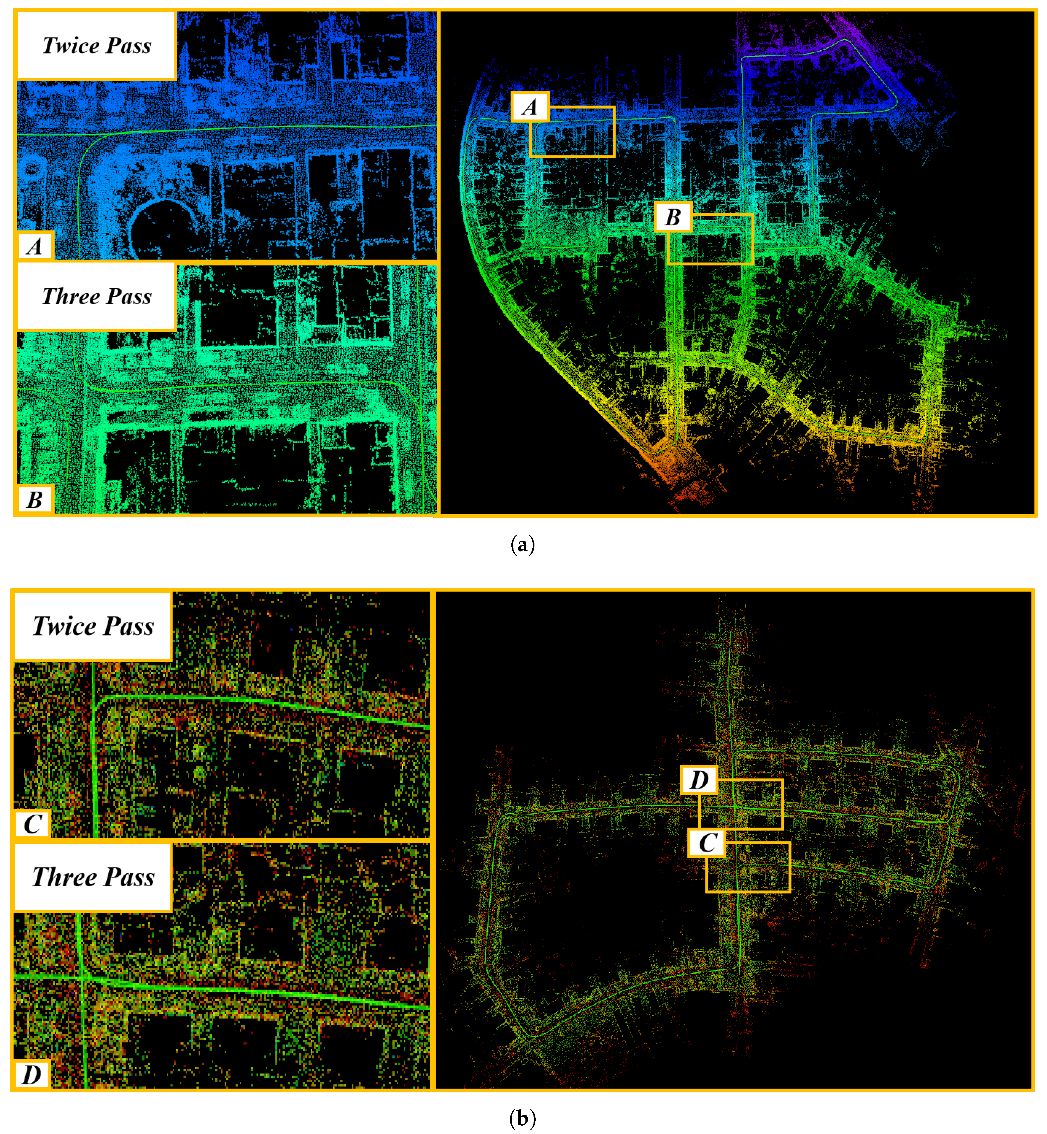
4.4. Mapping and Loop Closing Performance

This section evaluates the performance of VOX-LIOM in mapping and loop closing using kitti_00 and kitti_05. In Figure 13a, node A illustrates the mapping results after two passes through the same location, while node B shows the results after three passes along the same road section. For kitti_05, Figure 13b presents the mapping results at nodes C and D, which correspond to multiple passes through the same route. The results demonstrate that our algorithm effectively ensures global consistency in the overall mapping. The point cloud maps at all four nodes (A, B, C, D) exhibit minimal overlap, confirming the effectiveness of loop closing and pose-graph-based global optimization.

From the trajectory accuracy results in Table 3, we observe that incorporating global map optimization improves trajectory accuracy by 54.7% and 55.4% on kitti_00 and kitti_05, respectively, thereby ensuring the global consistency of the maps.

4.5. Generalization Experiments

In this section, we conduct experiments on two self-built mobile platforms: a four-wheeled mobile robot and a quadruped robot, to verify the applicability and effectiveness of the proposed algorithms.

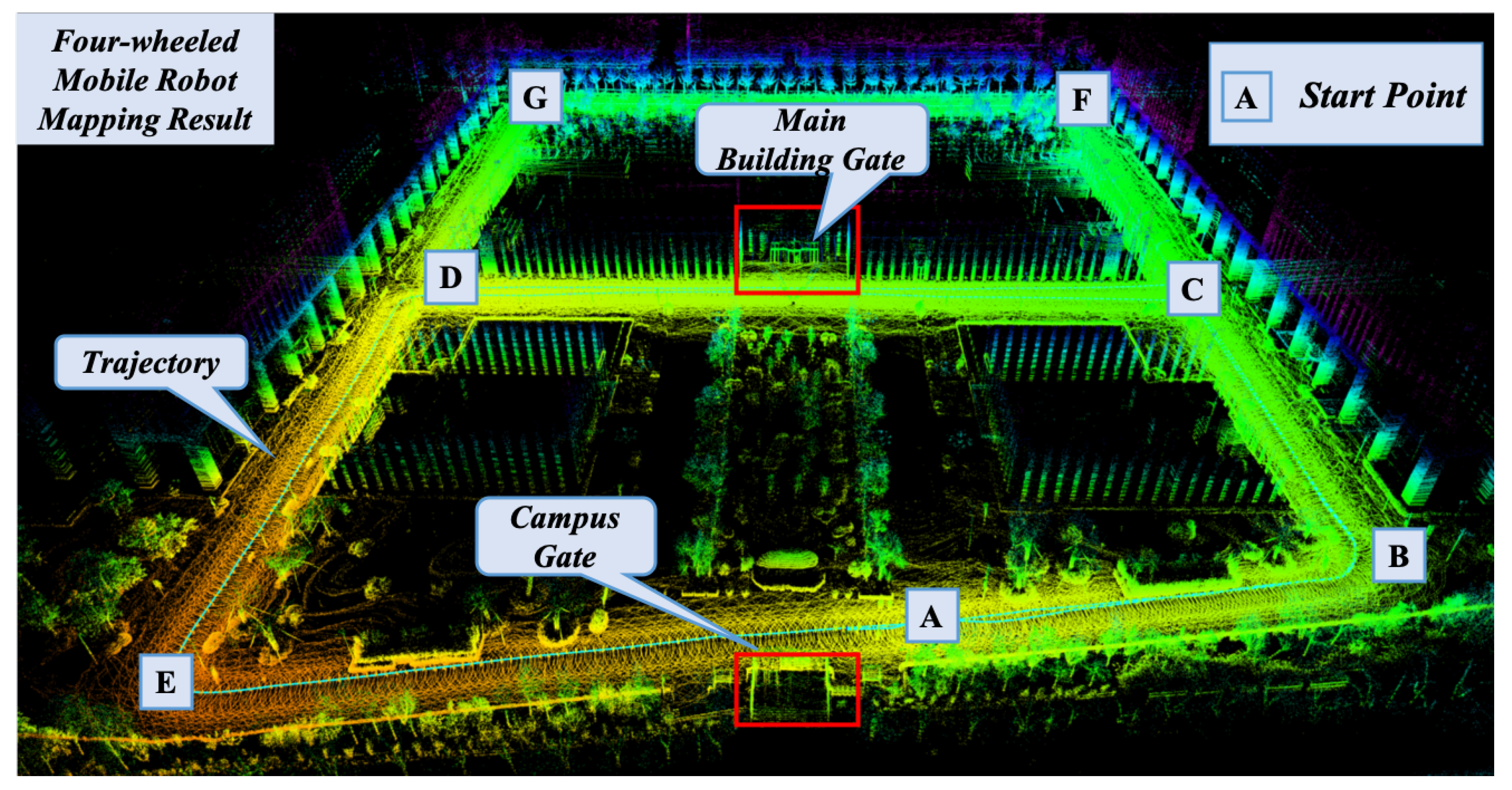
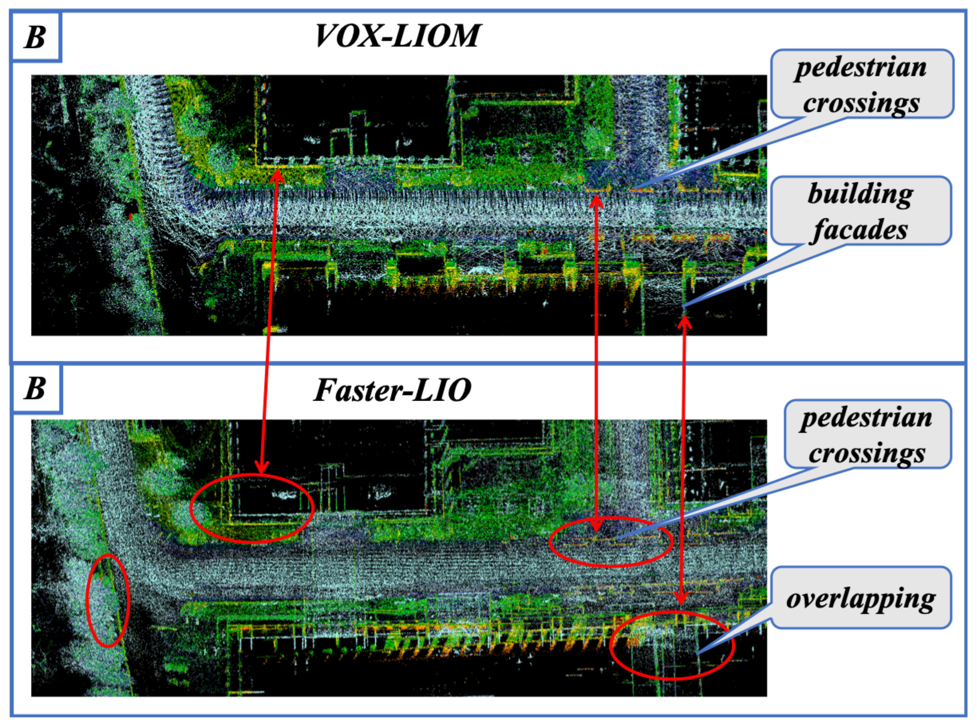
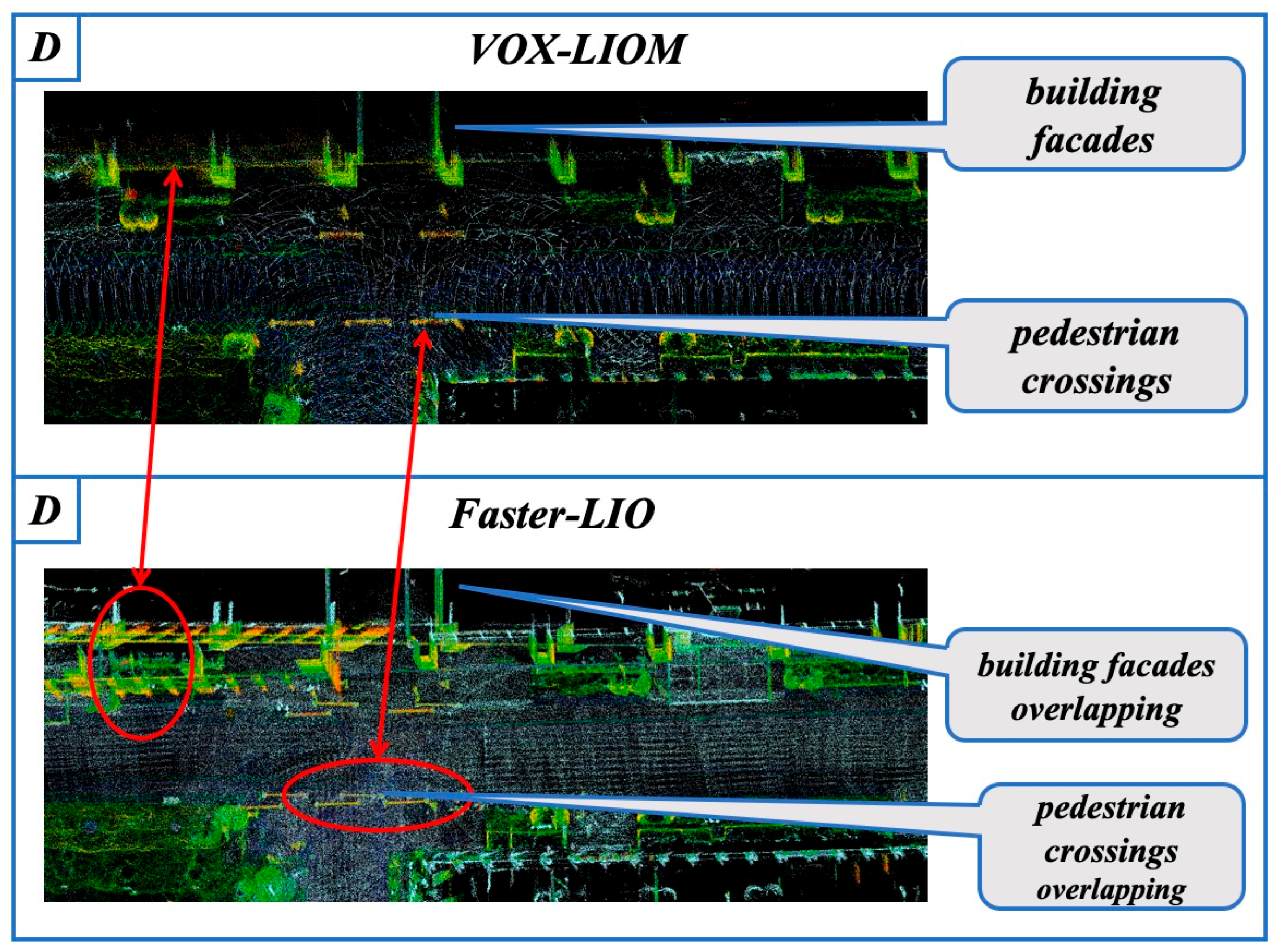
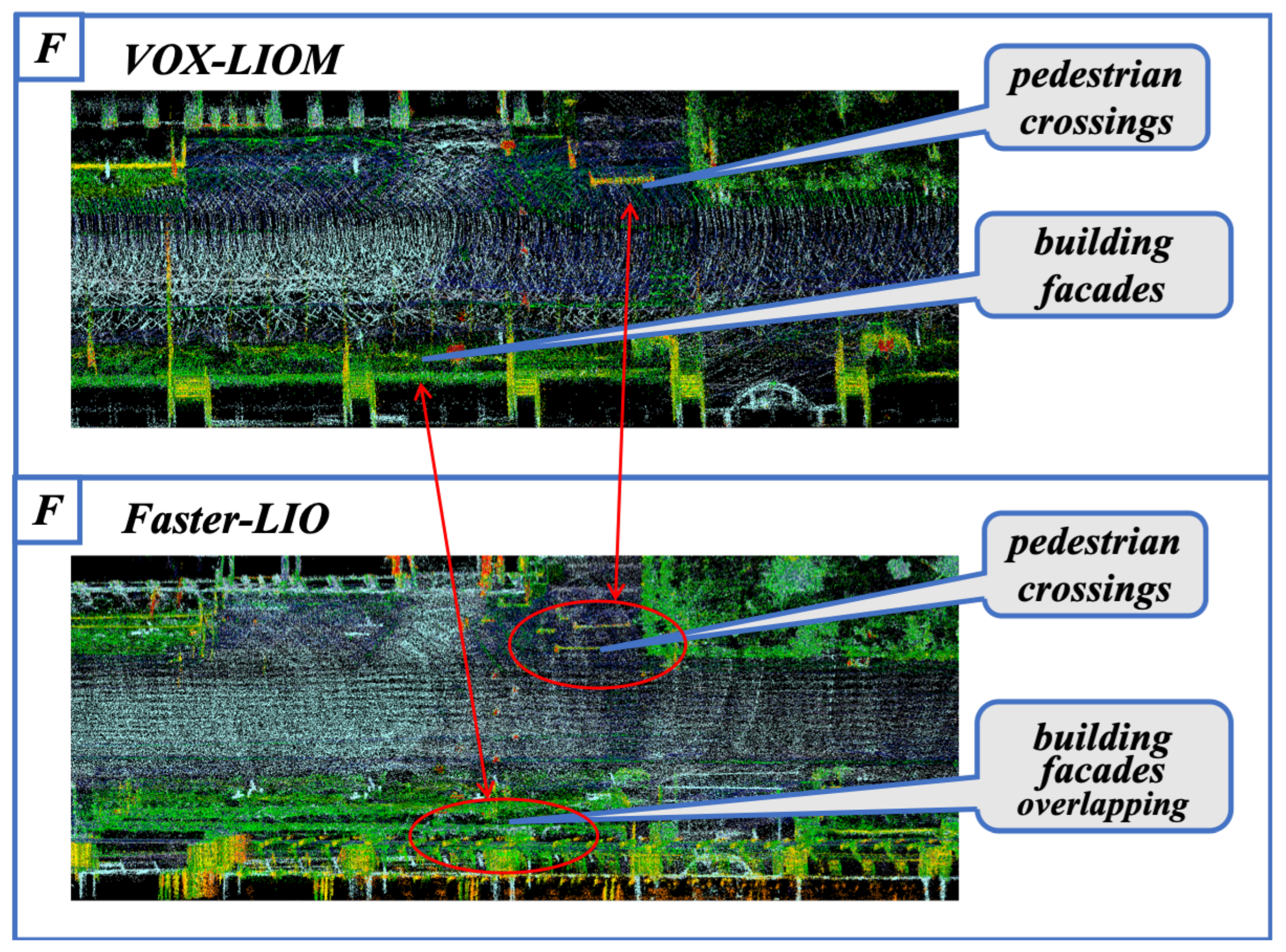
4.5.1. Experiments of the Four-Wheeled Robot Platform

The trajectory of the four-wheeled robot is shown in Figure 14, covering a total distance of 1.05 km over a patrol period of 27 min. The campus, densely populated with buildings, causes significant GNSS signal obstruction, making direct trajectory error evaluation impossible due to the lack of ground truth.

We marked waypoints and repeated the routes multiple times during the campus data collection, which allows us to evaluate the algorithm’s performance based on the global consistency of the generated map. For instance, along the $A\Rightarrow C$ road section in Figure 14, the four-wheeled robot was instructed to traverse the same route twice. Pose estimation accuracy is evaluated by checking whether the trajectories overlap and whether there is any overlap in the point cloud map.

The overall mapping result of the VOX-LIOM algorithm is shown in Figure 15, with detailed comparative maps at locations B, D, and F presented in Figure 16, Figure 17 and Figure 18. Since the robot passes through B, D, and F twice, the consistency of the maps at these locations serves as an indicator of the algorithm’s performance.

The map generated by VOX-LIOM clearly outlines pedestrian crossings and building facades without any noticeable “overlapping”. In contrast, the Faster-LIO map is blurred, with significant “overlapping” on building facades and pedestrian crossings, and lacks consistency in these areas.

The comparison of the trajectories between VOX-LIO, VOX-LIOM, and Faster-LIO is shown in Figure 19. As observed, the pose estimation of Faster-LIO in the z-axis direction exhibits significant error after extended operation, leading to noticeable drift in the overall trajectory. In contrast, VOX-LIOM more closely follows the actual motion trajectory of the robot, demonstrating better consistency.

Overall, VOX-LIOM, with its integration of loop closing and global optimization, successfully performs localization and mapping tasks on the four-wheeled robot platform.

4.5.2. Experiments of the Quadruped Robot Platform

To thoroughly evaluate the generality of our method, we conducted experiments on a quadruped robot platform, with the mapping results shown in Figure 20. Due to the more dynamic and bumpy movement of the quadruped robot, the point cloud data experiences more severe distortion, making it more reliant on the motion information provided by the IMU to maintain global consistency.

As seen in the map shown in Figure 20, while some slight dragging occurs, the localization and mapping task is still completed. In contrast, Fast-LOAM performs inadequately on the quadruped robot platform.

4.6. Efficiency Experiments

In addition to ensuring localization accuracy and robustness, achieving high computational efficiency is also critical for the real-time deployment of LiDAR-inertial odometry (LIO) systems on resource-constrained robotic platforms. In this section, we conduct comparative experiments with other representative methods in terms of both data association (matching) time and overall runtime, to validate the efficiency of the proposed approach.

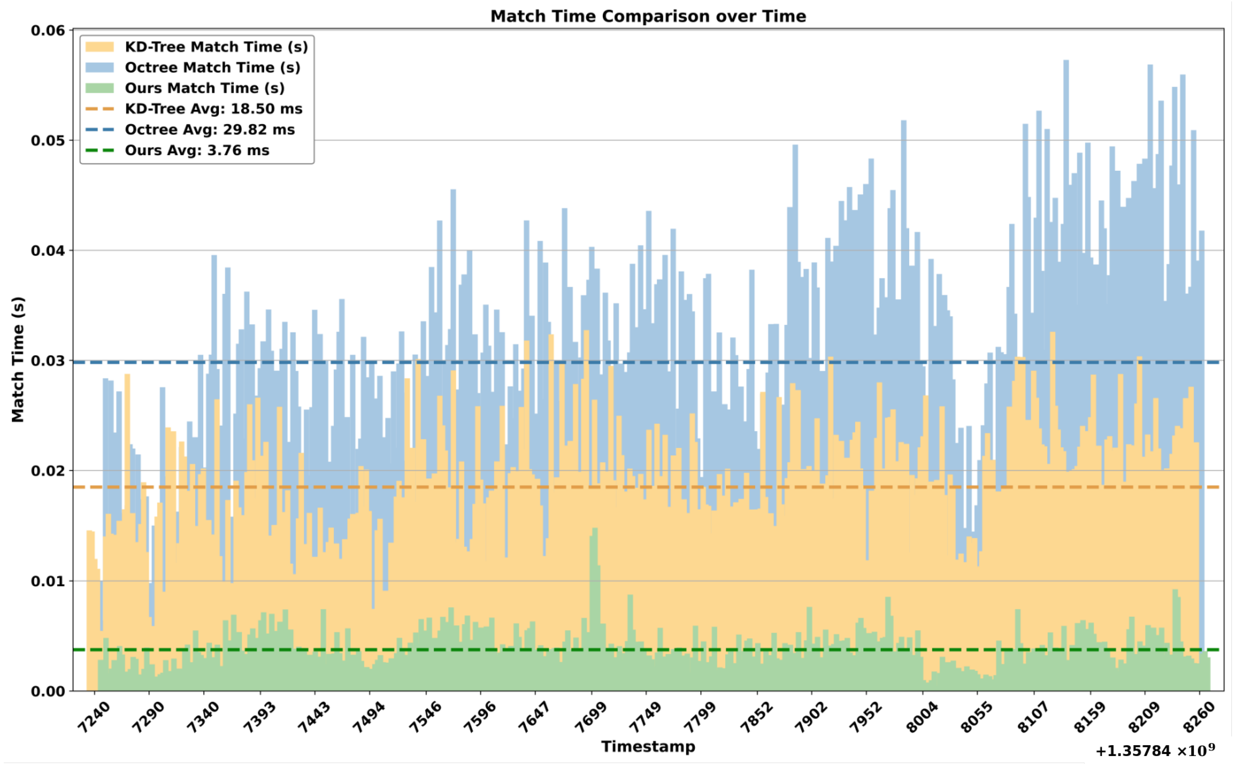
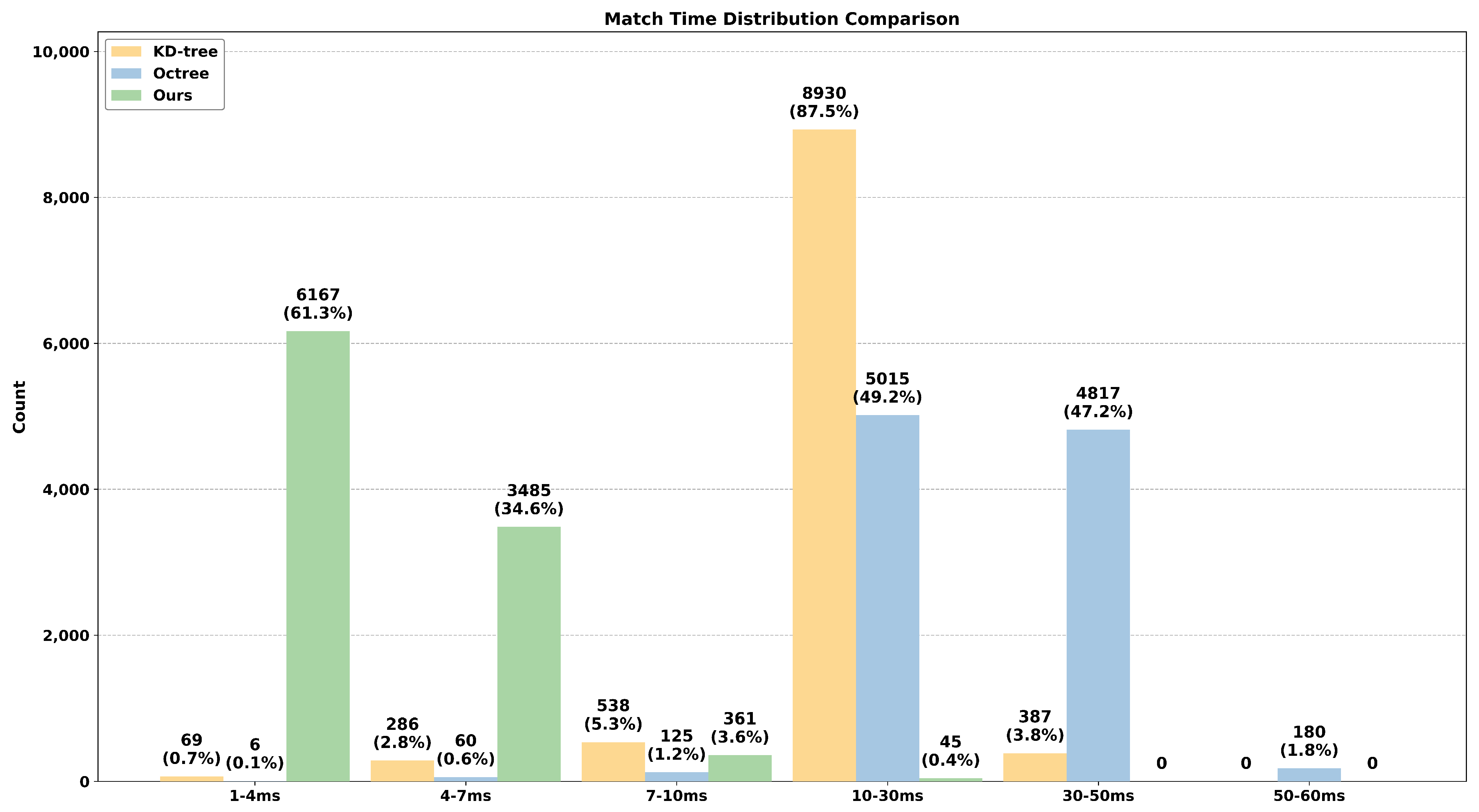
4.6.1. Surfel Voxel-Based Matching Efficiency

To evaluate the effectiveness of surfel voxel-based matching in improving system efficiency, we conducted a comparative experiment on nclt_01, benchmarking our method against KD-tree and Octree-based approaches. We present the comparative results in Figure 21 and Figure 22 to demonstrate the performance differences among the methods.

Our method achieves an average matching time of 3.76 ms, reflecting a substantial efficiency improvement over both KD-tree and Octree baselines. Moreover, as illustrated in Figure 22, 61.3% of the frame-wise matching times consistently fall within the 1–4 ms interval across the entire sequence, while only a negligible 0.4% lie in the 10–30 ms range, demonstrating both high efficiency and temporal stability of the proposed approach.

4.6.2. Surfel Voxel-Based Acceleration for Runtime Efficiency

To ensure the stable and reliable operation of mobile robots, runtime efficiency is a key consideration. We conducted comparative experiments using the NCLT dataset and a four-wheeled robot platform.

Table 4. Comparison results of algorithm operation efficiency analysis. “Pre.” indicates the time spent on point cloud preprocessing, and “Est.” represents the time spent on pose estimation.

Dataset	VOX-LIO		Faster-LIO		Fast-LOAM
	Pre. (ms)	Est. (ms)	Pre. (ms)	Est. (ms)	Pre. (ms)	Est. (ms)
nclt_01	6.60	13.08	6.8	20.78	6.71	37.23
nclt_02	6.25	11.45	6.35	17.89	5.87	35.29
Four-wheeled	5.80	12.27	5.72	18.17	5.61	27.16
Mean	6.22	12.26	6.29	18.95	6.06	33.23

presents the performance of VOX-LIO compared to Fast-LOAM and Faster-LIO, both baselines configured with a voxel size of 0.5 m.

The primary computational bottlenecks lie in feature extraction, point cloud downsampling, motion distortion compensation, and pose optimization. For clarity of analysis, we divide the per-frame processing time into two main stages: point cloud preprocessing and pose estimation.

Fast-LOAM, which utilizes a KD-tree for nearest-neighbor search, achieves a performance of around 26 Hz on computationally constrained platforms. However, due to the large volume of point cloud data, maintaining the KD-tree incurs considerable computational overhead, which limits its real-time efficiency compared to hash table–based methods.

Faster-LIO utilizes hash tables for nearest-neighbor search, which enhances retrieval efficiency to some extent. However, since it discretizes space and stores numerous points within each voxel, it cannot guarantee constant-time $O\left(1\right)$ time complexity. Moreover, redundant surfel fitting during plane estimation further degrades computational efficiency.

In contrast, our proposed algorithm classifies map voxels into surfel voxels and common voxels. For surfel voxels, planar features are pre-fitted using the stored point cloud data, thereby eliminating the need for redundant re-fitting of the same features during optimization. This design ensures an $O\left(1\right)$ time complexity for surfel feature retrieval, significantly accelerating the correspondence search process.

Benefiting from these designs, VOX-LIO significantly reduces redundant queries and achieves substantial improvements in runtime performance. As shown in Table 4, it yields an average runtime improvement of 26.78% over Faster-LIO and 53.0% over Fast-LOAM, operating at an average runtime frequency of 54.11 Hz across the three benchmark datasets.

5. Conclusions

To address the challenge of achieving real-time, high-precision LiDAR-inertial odometry on resource-constrained platforms, we proposed VOX-LIO. This robust and efficient mapping system combines adaptive surfel-based matching, manifold-based sensor fusion, and loop closure integration.

Our system introduces a point cloud matching strategy based on adaptive hash voxels that leverage surfel features and planarity, enabling accurate and efficient map updates through voxel classification and incremental surfel refinement. To compensate for motion distortion, we formulate LiDAR-IMU fusion as a weighted optimization problem on the manifold, enhancing estimation robustness under aggressive motion. Furthermore, a loop closure module is incorporated to correct long-term drift and maintain global map consistency.

Extensive experiments conducted on public datasets and real-world robotic platforms verify the effectiveness of VOX-LIO. Notably, on the kitti_05 sequence, VOX-LIOM reduces the mean absolute pose error (APE) by 55.5% compared to VOX-LIO, demonstrating significant improvements in both pose accuracy and global consistency. These results confirm the capability of VOX-LIOM to support real-time, scalable, and reliable mapping in various environments.

Looking ahead, we plan to incorporate visual sensor constraints into the manifold optimization framework. To enable this, we will address two critical challenges: extrinsic calibration and temporal synchronization between cameras and LiDAR sensors. These steps are essential for fully leveraging the complementary characteristics of multimodal sensor data and improving the robustness and accuracy of pose estimation.

Multi-sensor fusion poses several technical challenges. First, extrinsic calibration between heterogeneous sensors is non-trivial due to differences in coordinate systems, sensor modalities, and fields of view (FOV), all of which can introduce systematic errors. Second, temporal synchronization is especially crucial in dynamic scenes; even microsecond-level misalignments can cause significant spatial inconsistencies. The fusion of high-frequency IMU data with low-frequency LiDAR or camera inputs requires precise alignment mechanisms and interpolation strategies to ensure temporal consistency.

In addition, we aim to integrate semantic information, such as global descriptors or scene graphs, extracted from LiDAR or images, thereby enhancing semantic understanding and recognition. We also plan to investigate recent advancements in 3D Gaussian splatting (3DGS) for incremental and high-fidelity environmental reconstruction. Finally, the potential of large language models (LLMs) to support multimodal reasoning and knowledge-guided perception will be explored as part of our long-term goal of enabling higher-level semantic understanding.

References

1. Zhang, J.; Singh, S. LOAM: Lidar Odometry and Mapping in Real-time. In Proceedings of the Robotics: Science and Systems Conference, Berkeley, CA, USA, 12–13 July 2014; Volume 2, pp. 1–9. [Google Scholar]
2. Wang, H.; Wang, C.; Chen, C.; Xie, L. F-LOAM: Fast LiDAR Odometry And Mapping. arXiv 2021, arXiv:2107.00822. [Google Scholar]
3. Xu, W.; Zhang, F. Fast-lio: A fast, robust lidar-inertial odometry package by tightly-coupled iterated kalman filter. IEEE Robot. Autom. Lett. 2021, 6, 3317–3324. [Google Scholar] [CrossRef]
4. He, D.; Xu, W.; Zhang, F. Kalman Filters on Differentiable Manifolds. arXiv 2021, arXiv:2102.03804. [Google Scholar]
5. Shan, T.; Englot, B.J.; Meyers, D.; Wang, W.; Ratti, C.; Rus, D. LIO-SAM: Tightly-coupled Lidar Inertial Odometry via Smoothing and Mapping. arXiv 2020, arXiv:2007.00258. [Google Scholar]
6. Besl, P.J.; McKay, N.D. Method for registration of 3-D shapes. In Proceedings of the Sensor Fusion IV: Control Paradigms and Data Structures, Boston, MA, USA, 12–15 November 1992; Volume 1611, pp. 586–606. [Google Scholar]
7. Censi, A. An ICP variant using a point-to-line metric. In Proceedings of the 2008 IEEE International Conference on Robotics and Automation, Pasadena, CA, USA, 19–23 May 2008; pp. 19–25. [Google Scholar]
8. Serafin, J.; Grisetti, G. NICP: Dense normal based point cloud registration. In Proceedings of the 2015 IEEE/RSJ International Conference on Intelligent Robots and Systems (IROS), Hamburg, Germany, 28 September–3 October 2015; pp. 742–749. [Google Scholar]
9. Deschaud, J.E. IMLS-SLAM: Scan-to-model matching based on 3D data. In Proceedings of the 2018 IEEE International Conference on Robotics and Automation (ICRA), Brisbane, Australia, 21–25 May 2018; pp. 2480–2485. [Google Scholar]
10. Low, K.L. Linear Least-Squares Optimization for Point-To-Plane Icp Surface Registration; University of North Carolina: Chapel Hill, NC, USA, 2004; Volume 4, pp. 1–3. [Google Scholar]
11. Cho, H.; Kim, E.K.; Kim, S. Indoor SLAM application using geometric and ICP matching methods based on line features. Robot. Auton. Syst. 2018, 100, 206–224. [Google Scholar] [CrossRef]
12. Magnusson, M.; Andreasson, H.; Nuchter, A.; Lilienthal, A.J. Appearance-based loop detection from 3D laser data using the normal distributions transform. In Proceedings of the 2009 IEEE International Conference on Robotics and Automation, Kobe, Japan, 12–17 May 2009; pp. 23–28. [Google Scholar]
13. Shan, T.; Englot, B. Lego-loam: Lightweight and ground-optimized lidar odometry and mapping on variable terrain. In Proceedings of the 2018 IEEE/RSJ International Conference on Intelligent Robots and Systems (IROS), Madrid, Spain, 1–5 October 2018; pp. 4758–4765. [Google Scholar]
14. Behley, J.; Stachniss, C. Efficient Surfel-Based SLAM using 3D Laser Range Data in Urban Environments. In Proceedings of the Robotics: Science and Systems, Pittsburgh, PA, USA, 26–30 June 2018; Volume 2018, p. 59. [Google Scholar]
15. Chen, X.; Milioto, A.; Palazzolo, E.; Giguère, P.; Behley, J.; Stachniss, C. SuMa++: Efficient LiDAR-based Semantic SLAM. arXiv 2021, arXiv:2105.11320. [Google Scholar]
16. Skrodzki, M. The k-d tree data structure and a proof for neighborhood computation in expected logarithmic time. arXiv 2019, arXiv:1903.04936. [Google Scholar]
17. Cai, Y.; Xu, W.; Zhang, F. ikd-Tree: An incremental KD tree for robotic applications. arXiv 2021, arXiv:2102.10808. [Google Scholar]
18. Hess, W.; Kohler, D.; Rapp, H.; Andor, D. Real-time loop closure in 2D LIDAR SLAM. In Proceedings of the 2016 IEEE International Conference on Robotics and Automation (ICRA), Stockholm, Sweden, 16–21 May 2016; pp. 1271–1278. [Google Scholar]
19. Grisetti, G.; Stachniss, C.; Burgard, W. Improving grid-based slam with rao-blackwellized particle filters by adaptive proposals and selective resampling. In Proceedings of the 2005 IEEE International Conference on Robotics and Automation, Barcelona, Spain, 18–22 April 2005; pp. 2432–2437. [Google Scholar]
20. Aoki, Y.; Goforth, H.; Srivatsan, R.A.; Lucey, S. Pointnetlk: Robust & efficient point cloud registration using pointnet. In Proceedings of the IEEE/CVF Conference on Computer Vision and Pattern Recognition, Long Beach, CA, USA, 15–20 June 2019; pp. 7163–7172. [Google Scholar]
21. Kalman, R.E. A New Approach to Linear Filtering and Prediction Problems. Trans. ASME Ser. D. J. Basic Engrg. 1960, 82, 35–45. [Google Scholar] [CrossRef]
22. Qian, C.; Liu, H.; Tang, J.; Chen, Y.; Kaartinen, H.; Kukko, A.; Zhu, L.; Liang, X.; Chen, L.; Hyyppä, J. An integrated GNSS/INS/LiDAR-SLAM positioning method for highly accurate forest stem mapping. Remote Sens. 2016, 9, 3. [Google Scholar] [CrossRef]
23. Gao, J.; Sha, J.; Wang, Y.; Wang, X.; Tan, C. A fast and stable GNSS-LiDAR-inertial state estimator from coarse to fine by iterated error-state Kalman filter. Robot. Auton. Syst. 2024, 175, 104675. [Google Scholar] [CrossRef]
24. Dellaert, F.; Fox, D.; Burgard, W.; Thrun, S. Monte carlo localization for mobile robots. In Proceedings of the 1999 IEEE International Conference on Robotics and Automation (Cat. No. 99CH36288C), Detroit, MI, USA, 10–15 May 1999; Volume 2, pp. 1322–1328. [Google Scholar]
25. Ye, H.; Chen, Y.; Liu, M. Tightly coupled 3d lidar inertial odometry and mapping. In Proceedings of the 2019 International Conference on Robotics and Automation (ICRA), Montreal, Canada, 20–24 May 2019; pp. 3144–3150. [Google Scholar]
26. Lin, J.; Zhang, F. R3LIVE: A Robust, Real-time, RGB-colored, LiDAR-Inertial-Visual tightly-coupled state Estimation and mapping package. arXiv 2021, arXiv:2109.07982. [Google Scholar]
27. Kim, G.; Kim, A. Scan context: Egocentric spatial descriptor for place recognition within 3d point cloud map. In Proceedings of the 2018 IEEE/RSJ International Conference on Intelligent Robots and Systems (IROS), Madrid, Spain, 1–5 October 2018; pp. 4802–4809. [Google Scholar]
28. Wang, Y.; Sun, Z.; Xu, C.Z.; Sarma, S.E.; Yang, J.; Kong, H. Lidar iris for loop-closure detection. In Proceedings of the 2020 IEEE/RSJ International Conference on Intelligent Robots and Systems (IROS), Las Vegas, NV, USA, 25–29 October 2020; pp. 5769–5775. [Google Scholar]
29. Konolige, K.; Grisetti, G.; Kümmerle, R.; Burgard, W.; Limketkai, B.; Vincent, R. Efficient sparse pose adjustment for 2D mapping. In Proceedings of the 2010 IEEE/RSJ International Conference on Intelligent Robots and Systems, Taipei, Taiwan, 18–22 October 2010; pp. 22–29. [Google Scholar]
30. Dellaert, F.; Kaess, M. Square root SAM: Simultaneous localization and mapping via square root information smoothing. Int. J. Robot. Res. 2006, 25, 1181–1203. [Google Scholar] [CrossRef]
31. Yin, H.; Xu, X.; Lu, S.; Chen, X.; Xiong, R.; Shen, S.; Stachniss, C.; Wang, Y. A Survey on Global LiDAR Localization: Challenges, Advances and Open Problems. arXiv 2024, arXiv:2302.07433. [Google Scholar] [CrossRef]
32. Daun, K.; Kohlbrecher, S.; Sturm, J.; von Stryk, O. Large scale 2d laser slam using truncated signed distance functions. In Proceedings of the 2019 IEEE International Symposium on Safety, Security, and Rescue Robotics (SSRR), Wurzburg, Germany, 2–4 September 2019; pp. 222–228. [Google Scholar]
33. Teschner, M. Optimized Spatial Hashing for Collision Detection of Deformable Objects. VMV 2003, 3, 47–54. [Google Scholar]
34. Yuan, C.; Xu, W.; Liu, X.; Hong, X.; Zhang, F. Efficient and probabilistic adaptive voxel mapping for accurate online lidar odometry. IEEE Robot. Autom. Lett. 2022, 7, 8518–8525. [Google Scholar] [CrossRef]
35. Cui, Y.; Zhang, Y.; Dong, J.; Sun, H.; Zhu, F. Link3d: Linear keypoints representation for 3d lidar point cloud. arXiv 2022, arXiv:2206.05927. [Google Scholar] [CrossRef]
36. Geiger, A.; Lenz, P.; Stiller, C.; Urtasun, R. Vision meets Robotics: The KITTI Dataset. Int. J. Robot. Res. 2013, 32, 1231–1237. [Google Scholar] [CrossRef]
37. Carlevaris-Bianco, N.; Ushani, A.K.; Eustice, R.M. University of Michigan North Campus long-term vision and lidar dataset. Int. J. Robot. Res. 2015, 35, 1023–1035. [Google Scholar] [CrossRef]
38. Grupp, M. evo: Python Package for the Evaluation of Odometry and SLAM. 2017. Available online: https://github.com/MichaelGrupp/evo (accessed on 13 May 2025).
39. Feng, Y.; Jiang, Z.; Shi, Y.; Feng, Y.; Chen, X.; Zhao, H.; Zhou, G. Block-Map-Based Localization in Large-Scale Environment. In Proceedings of the 2024 IEEE International Conference on Robotics and Automation (ICRA), Yokohama, Japan, 13–17 May 2024; pp. 1709–1715. [Google Scholar] [CrossRef]
Figure 1. Overview of our method. The LiDAR point cloud is first downsampled using voxel filtering and then motion-compensated with high-frequency IMU measurements. The undistorted point cloud is then matched with surfel features for pose estimation through weighted nonlinear optimization on the manifold, incorporating both geometric and inertial constraints. Each estimated pose and completed submap is passed to the loop closure module, which performs line feature-based matching and triggers global pose graph optimization upon successful loop detection. The dotted arrow is optional.
Remotesensing 17 02214 g001
Figure 2. Surfel feature fitting illustration.
Remotesensing 17 02214 g002
Figure 3. Schematic of hash voxel mapping. For any point in the point cloud, the voxel index in continuous space is first computed based on its world coordinates. This index is then mapped to a hash bucket using a hash function (e.g., H ( x , y , z ) , see Equation (3)). To resolve collisions, separate chaining is employed. Each spatial voxel that contains at least one point subsequently points to a surfel voxel structure.
Remotesensing 17 02214 g003
Figure 4. Maintenance of local submap.
Remotesensing 17 02214 g004
Figure 5. Illustration of the 18 spatially nearest voxels in continuous space. The center voxel is surrounded by six face-adjacent voxels, as shown in (a), and 12 edge-adjacent voxels, as shown in (b), forming its immediate spatial neighborhood. This 3D configuration excludes corner-adjacent voxels and is employed for local surfel and point association during the mapping process.
Remotesensing 17 02214 g005
Figure 6. Illustration of the pose graph structure for global optimization.
Remotesensing 17 02214 g006
Figure 7. Self-built mobile robot platforms. (a) The four-wheeled mobile robot. (b) The quadruped mobile robot.
Remotesensing 17 02214 g007
Figure 8. Trajectory estimation comparison on kitti_00 using Fast-LOAM, VOX-LIO, and VOX-LIOM.
Remotesensing 17 02214 g008
Figure 9. Trajectory estimation comparison on kitti_05 using different methods. The top row shows results from Fast-LIO, LIO-SAM without loop closure, and LIO-SAM with loop closure. The bottom row shows results from Faster-LIO, VOX-LIO, and VOX-LIOM.
Remotesensing 17 02214 g009
Figure 10. Trajectory estimation results for the nclt_01 sequence using different methods. The top row displays 2D trajectories in the x–y plane, while the bottom row presents absolute trajectory error (ATE) curves over time.
Remotesensing 17 02214 g010
Figure 11. Trajectory estimation on the nclt_02 based on Faster-LIO and VOX-LIO.
Remotesensing 17 02214 g011
Figure 12. The mapping result of the NCLT dataset.
Remotesensing 17 02214 g012
Figure 13. Mapping consistency after loop closing for (a) kitti_00 and (b) kitti_05, showing minimal overlap at repeated locations.
Remotesensing 17 02214 g013
Figure 14. Driving route of the four-wheeled mobile robot.
Remotesensing 17 02214 g014
Figure 15. The whole mapping result of a four-wheeled mobile robot.
Remotesensing 17 02214 g015
Figure 16. Comparison of BC Location Mapping Results.
Remotesensing 17 02214 g016
Figure 17. Comparison of D Location Mapping Results.
Remotesensing 17 02214 g017
Figure 18. Comparison of F Location Mapping Results.
Remotesensing 17 02214 g018
Figure 19. Trajectory and speed comparison of the four-wheeled mobile robot. (a) Trajectory comparison among VOX-LIO, VOX-LIOM, and Faster-LIO. (b) Speed profiles in x, y, and z axes for the three methods.
Remotesensing 17 02214 g019
Figure 20. Overall mapping performance of the quadruped robot platform evaluated at the Beijing Institute of Technology (BIT).
Remotesensing 17 02214 g020
Figure 21. Comparison of average matching time among different methods on nclt_01.
Remotesensing 17 02214 g021
Figure 22. Distribution of frame–wise matching times across the sequence.
Remotesensing 17 02214 g022