Assessment of Remote Sensing Reflectance Glint Correction Methods from Fixed Automated Above-Water Hyperspectral Radiometric Measurement in Highly Turbid Coastal Waters

Abstract

Fixed automated (unmanned) above-water radiometric measurements are subject to unavoidable sky conditions and surface perturbations, leading to significant uncertainties in retrieved water surface remote sensing reflectances (R_rs(λ), sr⁻¹). This study evaluates various above-water R_rs(λ) glint correction methods using a comprehensive dataset collected at the Royal Netherlands Institute for Sea Research (NIOZ) Jetty Station located in the Marsdiep tidal inlet of the Dutch Wadden Sea, the Netherlands. The dataset includes in-situ water constituent concentrations (2006–2020), inherent optical properties (IOPs) (2006–2007), and above-water hyperspectral (ir)radiance observations collected every 10 min (2006–2023). The bio-optical models were validated using in-situ IOPs and utilized to generate glint-free remote sensing reflectances, R_rs,ref(λ), using a robust IOP-to-R_rs forward model. The R_rs,ref(λ) spectra were used as a benchmark to assess the accuracy of glint correction methods under various environmental conditions, including different sun positions, wind speeds, cloudiness, and aerosol loads. The results indicate that the three-component reflectance model (3C) outperforms other methods across all conditions, producing the highest percentage of high-quality R_rs(λ) spectra with minimal errors. Methods relying on fixed or lookup-table-based glint correction factors exhibited significant errors under overcast skies, high wind speeds, and varying aerosol optical thickness. The study highlights the critical importance of surface-reflected skylight corrections and wavelength-dependent glint estimations for accurate above-water R_rs(λ) retrievals. Two showcases on chlorophyll-a and total suspended matter retrieval further demonstrate the superiority of the 3C model in minimizing uncertainties. The findings highlight the importance of adaptable correction models that account for environmental variability to ensure accurate R_rs(λ) retrieval and reliable long-term water quality monitoring from hyperspectral radiometric measurements.

1. Introduction

Remote Sensing Reflectance (R_rs(λ), sr⁻¹) is a crucial quantity in ocean color remote sensing tasks, which is necessary to develop water quality algorithms and evaluate the efficiency of the atmospheric correction algorithms [1,2,3]. Accurate estimation of R_rs(λ) is essential for reliable retrievals of water constituents such as Chlorophyll-a (Chla, mg m⁻³), Suspended Particulate Matter (SPM, g m⁻³), and Colored Dissolved Organic Matter (CDOM) [4,5,6]. However, the retrieval of R_rs(λ) from above-water radiometric measurements is particularly sensitive to environmental interferences, notably sky and sun glint, which can introduce substantial errors if not properly corrected [7,8,9]. In highly turbid coastal waters, the challenges of obtaining accurate R_rs(λ) values are amplified. These environments are characterized by complex light interactions due to elevated concentrations of particulates, dynamic surface roughness, and highly variable atmospheric conditions [10,11,12,13]. As a result, standard glint correction methods—particularly those relying on fixed geometry or lookup tables—often fail to provide consistent performance across varying observation conditions.

Despite growing attention to glint correction techniques in recent years, few studies have rigorously evaluated their performance over long-term, high-frequency above-water hyperspectral datasets in turbid coastal environments. Internationally, much of the literature has focused on ideal conditions or oceanic waters with relatively low turbidity [2,14,15,16], while dynamic coastal systems remain limited [11,17]. This study seeks to address these gaps by evaluating and comparing glint correction methods using an extensive multi-year dataset from a fixed automated station in the Dutch Wadden Sea.

In the field, R_rs(λ) is calculated as the ratio of water-leaving radiance (L_W(λ), mW m⁻² nm⁻¹ sr⁻¹) to downwelling irradiance (E_d, mW m⁻² nm⁻¹) just above the air-sea interface [14]. L_W(λ) contains information on inherent optical properties (IOPs) such as absorption (a(λ), m⁻¹) and backscattering (b_b(λ), m⁻¹) which are controlled by Water Constituents Concentrations (WCCs) and their types in the water column [18]. In-situ measurements of L_W(λ) are challenging due to specular reflections caused by surface-reflected light originating from the water surface [19]. The skylight-blocked approach (SBA) method has been utilized to measure L_W(λ) in the field. The SBA can measure L_W(λ) with high precision across different water types, but it is susceptible to uncertainties caused by self-shading, floating structure, and marine bio-fouling [19,20,21]. In contrast, L_W(λ) can be easily determined from above-water measurements using low-cost instruments and over long periods of time [15,22]. The above-water measurements include downwelling irradiance, upward radiance, and reflected sky radiance, which are measured simultaneously. In this way, the resulting L_W(λ) is influenced by sensor viewing angle (θ_V), sensor viewing azimuth (φ_V), solar zenith angle (θ_S), solar azimuth (φ_S), wind-induced surface roughness, and sky conditions (e.g., cloudiness) [14,23,24]. Both above- and in-water measurements have their advantages and disadvantages for accurate estimations of R_rs(λ) [25,26]. In the following, we focus on above-water measurements.

Automated above-water hyperspectral radiometry in a fixed station is a cost-effective solution that provides long time series of measurements. This type of measurement records the solar planar downwelling irradiance (E_d(λ), mW m⁻² nm⁻¹), and sky (L_S(λ), mW m⁻² nm⁻¹ sr⁻¹) and surface (L_T(λ), mW m⁻² nm⁻¹ sr⁻¹) radiances in short time steps (i.e., minutes or seconds) simultaneously. However, atmospheric conditions have a significant impact on E_d(λ) and L_S(λ), and water surface roughness affects the L_T(λ). Both factors introduce considerable uncertainty to R_rs(λ). To overcome this problem, researchers have developed various methods, which can be estimated through bio-optical modeling [16,17] or through a similarity spectrum approach [27]. In this way, R_rs(λ) is calculated from simultaneous measurements of E_S, L_S, and L_T as follows [8,14]:

$$R_{rs}\left(\mathsf{\lambda },{\theta }_v,{\mathsf{\Delta }\phi }_v\right)={\displaystyle \frac{L_T(\mathsf{\lambda },{\theta }_v,\mathsf{\Delta }\phi )}{E_d\left(\mathsf{\lambda }\right)}}-\rho \left({\theta }_v,\mathsf{\Delta }\phi \right){\displaystyle \frac{L_S\left(\mathsf{\lambda },{\pi -\theta }_v,\mathsf{\Delta }\phi \right)}{E_d\left(\mathsf{\lambda }\right)}}-∆L$$

(1)

where the geometry factor of (θ_V, Δφ) indicates the directions seen by the radiometer. ρ(θ_V,Δφ) (dimensionless, dl) is the effective surface reflectance that rescales the sky radiance to the reflected sea surface radiance. It is assumed that it is independent of the wavelength [7,14,28,29] or dependent on the wavelength [2,30,31]. ΔL (sr⁻¹) denoted the reflectance offset due to the residual glint contributions and/or variabilities of E_d(λ) and L_S(λ) that are not consistent with L_T(λ). For a flat surface, ρ(θ_V, φ_V) equals the Fresnel reflectance of the sea surface. Various approaches have been suggested for estimating ρ, including: fixed ρ values [4,29,32], sky-conditions-dependent ρ values [10], lookup tables of ρ(θ_V,Δφ) for various directional factors and wind speeds [14,33], and wavelength-dependent values of ρ(λ,θ_V,Δφ) for various directional factors, wind speeds, and aerosol loads [30]. However, a sensor geometry with θ_V = 40° and φ = 90°–135° is considered optimal to minimize glint perturbations [14], so in practice these geometries are usually fixed. Similarly, researchers have considered different approaches to estimate the ΔL, including a fixed value equal to the R_rs(λ) at Near Infra-Red (NIR) [34,35,36,37], values of the similarity spectrum at NIR [27], the difference between bio-optical models and simulated R_rs(λ) [16], and estimating the direct surface reflected radiance to simulate ΔL [7,28]. The last approach substitutes a wavelength-dependent correction factor of ΔL(λ) in Equation (1). Since automated above-water radiometry is subject to unavoidable varying environmental conditions, application of above-water radiometric measurements introduces additional challenges. Consequently, there is a need for a thorough review and assessment of methods because the estimates ρ and ΔL may not be accurate enough for long time series of measurements in all environmental conditions.

The analytical methods for deriving IOPs from R_rs(λ) comprise inverse modeling that cannot be exactly reduced to an analytical equation or expression and relies on empirical and/or semi-empirical relationships [1]. However, The Radiative Transfer (RT) simulations and the quasi-single scattering approximation (QSSA) forward models have been developed to estimate R_rs(λ) as a function of spectral IOPs [18]. Several forward QSSA analytical expressions have been developed that estimate the R_rs(λ) as a function of a(λ), m⁻¹) and b_b(λ) [18,38,39]. Similarly, RT models simulate R_rs(λ) as a function of user-input IOPs and environmental parameters [14,38,40]. Therefore, RT and QSSA forward models explicitly relate IOPs to R_rs(λ) free of sun and sky glint. The resulting R_rs(λ) can be used as a reference to evaluate the above-water R_rs(λ) from Equation (1). In this regard, the lack of IOPs is a critical factor that significantly impacts the outcomes of this study. The validated regional bio-optical models can be utilized to overcome the lack of IOPs data [18].

This research aims to evaluate the performance of various sun, sky, and surface glint correction models from fixed automated above-water radiometric measurements in highly turbid coastal waters. To overcome the limitations of in-situ IOPs, this study also integrates validated bio-optical models to simulate glint-free reference R_rs(λ) spectra, serving as a benchmark for evaluating different correction techniques. The analytical forward models used here provide a physically based representation of R_rs(λ) as a function of IOPs and water constituent concentrations. This study aims to evaluate the performance of multiple glint correction models—including both empirical and semi-analytical approaches—under a wide range of environmental conditions. Finally, we provide evidence through two practical showcases (Chla and SPM) that highlight the real-world impact of glint correction accuracy.

2. Field Data

2.1. Above-Water Hyperspectral Radiometric Data

We utilized a time series of above-water hyperspectral measurements spanning from 2006 to 2023 at the Royal Netherlands Institute for Sea Research (NIOZ) jetty station (NJS) located near the Marsdiep tidal inlet of the Dutch Wadden Sea (Figure 1a). NJS has been equipped with a set of 6 TRIOS-RAMSES radiometers, comprising 1 Ramses-ACC for measuring solar downwelling irradiance (E_d, mW m⁻² nm⁻¹), 1 Ramses ACC-UV for measuring solar downwelling irradiance in the ultraviolet region (E_S-UV, mW m⁻² nm⁻¹), 2 pairs of Ramses-ARC for measuring sky radiance (L_S, mW m⁻² nm⁻¹ sr⁻¹), and total upwelling radiance from water surface (L_T, mW m⁻² nm⁻¹ sr⁻¹). The spectral data was recorded every 10 min at 1 nm intervals, ranging from 350 nm to 950 nm. The ARC sensors were mounted with fixed viewing angle θ_V = 35° and direction φ_V = 135° (south-east) and φ_V = 225° (south-west) (Figure 1b–d), following the optimized method recommended by [4]. All radiometric measurements were acquired using standard cosine collectors and factory-supplied optics. A set of quality control tests was applied to the hyperspectral data to flag the invalid or suspicious spectra [41]. The quality-controlled flagged spectra were excluded from further analysis. In this study, we used the quality-controlled E_d(λ), L_S(λ), and L_T(λ) covering 6:00 AM to 6:00 PM (UTC).

2.2. Meteorological Data

Hourly meteorological observations from the De Kooy station (Figure 1), located approximately 8 km southwest of NJS, covering the period from 2006 to 2023, were obtained from The Royal Netherlands Meteorological Institute (KNMI) database (https://dataplatform.knmi.nl). Measurements included cloud cover (CC, coverage of the upper sky in eighths, with ‘9’ indicating the upper sky invisible), atmospheric pressure (hPa), relative humidity (%), and wind speed (m s⁻¹).

2.3. IOPs Data

Reference [32] measured IOPs at 156 stations across the entire Wadden Sea between 2006 and 2007. Of these, 22 stations collected at NJS during March, June, and July 2006 were used in this study (hereafter referred to as HA09). The HA09’s IOPs dataset included laboratory spectrophotometry of total absorption (a(λ), m⁻¹), Colored Dissolved Organic Matter (CDOM) absorption (a_CDOM(λ), m⁻¹), particle absorption (ap(λ), m⁻¹), Non-Algal Particle (NAP) absorption (a_NAP(λ), m⁻¹), and phytoplankton absorption (a_Phy(λ), m⁻¹). They have measured particle absorption with a spectrophotometer (Ocean Optics) using the filter pad method. In addition, beam attenuation (c(λ), m⁻¹) and total absorption were measured in-field using an AC9 (Wet Labs, 25 cm cuvette, linearity range 0.001–30 m⁻¹), hereafter c_AC9(λ) and a_AC9(λ). The AC9 operated at nine standard wavelengths (412, 440, 488, 510, 555, 630, 650, 676, and 750 nm) ([32], their Table 2). Both in-situ and ex-situ measurements were conducted based on standard protocols [42], corrected for blank measurements on MilliQ water, and corrected for temperature-salinity and scattering [43], respectively. Only the AC9 data at depth ≤ 1.0 m were utilized, along with spectrophotometer data. The particle scattering was calculated as b_p(λ) = c_AC9(λ) − a_AC9(λ) for in-situ AC9 data. The light backscattering coefficients of particles were determined as follows [40,44]:

$$b_{bp}\left(\mathsf{\lambda }\right)=b_p\left(\mathsf{\lambda }\right)\times B$$

(2)

where B is the backscattering probability (or backscattering ratio), assumed to be spectrally constant [45,46]. The values of B ranged between 0.024 and 0.042 for surface waters of the coastal area of the English Channel [47]. The value of B has been assumed to be 0.026 in the Wadden Sea (Please see Supplementary, Section S1). Additionally, reference [48] proposed the B = 0.03 in the study area. Meanwhile, the sensitivity of modeled R_rs(λ) to variations in B was analyzed and found to be less than ±0.0015 sr⁻¹, well below the inter-model differences observed in the study area.

The HA09 dataset also included supplementary in-situ data of wind speed (m s⁻¹), water temperature (°C), Ph, salinity (PSU), Secchi Disk Depth (SDD, m⁻¹), and wave height (m).

2.4. Concentrations of Chla and SPM

A total of 1015 surface water samples were collected at NJS during 2006–2020 for laboratory Chla and SPM measurements. Of these, 648 samples included measurements of both Chla and Total Suspended Matter (TSM, g m⁻³). The Chla concentrations of the NJS dataset included two groups of High-Performance Liquid Chromatography (HPLC) and Fluorometry measurements. The Chla concentrations of HA09 and NJS-HPLC samples were measured using standard HPLC measurements on samples filtered through GF/F filters, then frozen and transported to laboratories for analysis. The Chla concentrations of NJS-Fluorometry samples were measured using a laboratory Fluorometer on filtered samples using standard methods by [49]. TSM concentrations were measured using the standard filtration method described by [42] using pre-ashed, rinsed, and weighted 47 mm GF/F filters. Readers are referred to [4,32] for more details on these measurements.

For validation purposes, each sample was matched to the nearest available quality-controlled above-water radiometric measurement within a ±10-min time window. Given the slow diurnal dynamics of Chla at the NIOZ Jetty Station [24,28], this matching approach introduces only minimal temporal uncertainty and does not significantly impact model evaluation.

3. Methods

3.1. Bio-Optical Models

IOPs are expressed as the sum of absorption or scattering by water molecules and various dissolved and particulate water components [50]. CDOM, NAP, and phytoplankton are the representatives of the natural water particles with distinct absorption and backscattering. The total absorption (a(λ), m⁻¹) and backscattering (b_b(λ), m⁻¹) coefficients of water can be expressed as follows [1,51]:

$$a\left(\mathsf{\lambda }\right)=a_w\left(\mathsf{\lambda }\right)+a_{Phy}\left(\mathsf{\lambda }\right)+a_{CDOM}\left(\mathsf{\lambda }\right)+a_{NAP}\left(\mathsf{\lambda }\right)$$

(3)

$$b_b\left(\mathsf{\lambda }\right)=b_{b,w}\left(\mathsf{\lambda }\right)+b_{b,Phy}\left(\mathsf{\lambda }\right)+b_{b,NAP}\left(\mathsf{\lambda }\right)$$

(4)

where the subscripts w, Phy, CDOM, and NAP represent contributions by pure water, phytoplankton, CDOM, and NAP constituents. Since CDOM backscattering is negligible, it is left out in Equation (4). The total non-water absorption (a_nw, m⁻¹) and particulate backscattering (b_bp, m⁻¹) are expressed as the sum of the non-water constituents: $a_{nw}\left(\mathsf{\lambda }\right)=a_{Phy}\left(\mathsf{\lambda }\right)+a_{CDOM}\left(\mathsf{\lambda }\right)+a_{NAP}\left(\mathsf{\lambda }\right)$, $b_{bp}\left(\mathsf{\lambda }\right)=b_{b,Phy}\left(\mathsf{\lambda }\right)+b_{b,NAP}\left(\mathsf{\lambda }\right)$.

Table 1. Methods of absorption and backscattering parametrization.

Variable	Sym.	Parametrization	Equation	Ref.
Chla-specific absorption	a*Chla	a* Chla(λ) = aPhy(λ)/[Chla]	(5)	[52]
Phy absorption	aPhy	aPhy(λ) = [Chla].a*Chla(λ)	(6)	[52]
Phy absorption a	aPhy	aPhy(λ) = [a0(λ) + a1(λ) × ln(aPhy(λ1))] × aPhy(λ1) a aPhy(λ1) = 0.06 × [Chla]0.65	(7)	[53]
CDOM absorption	aCDOM	aCDOM(λ) = aCDOM(λ2) × exp[−SCDOM × (λ − λ2)]	(8)	[54]
NAP absorption	aNAP	aNAP(λ) = aNAP(λ2) × exp[−SNAP × (λ − λ2)]	(9)	[54]
Chla backscattering	bb,Chla	bb,Chla(λ) = {0.002 + 0.02 × [0.5 − 0.25 × log10[Chla] × (λ3/λ)]} × bb,Chla(λ3), bb,Chla(λ3) = 0.416 × [Chl]0.766	(10)	[39]
Chla backscattering b	bb,Chla	bb,Chla(λ) = [Chla] × b*b,Chla(λ3) × bNChla(λ)	(11)	[55]
NAP backscattering c	bb,NAP	bb,NAP(λ) = bNAP(λ3) × (λ3/λ)γ − [1 − tanh(0.5 × γ2)] × aNAP(λ) bNAP(λ3) = b*SPM(λ3) × I × [SPM]	(12)	[56]
NAP backscattering d	bb,NAP	bb,NAP(λ) = [SPM] × b*b,SPM(λ) × bNNAP(λ) b*b,SPM(λ) = A × [SPM]B, bNNAP(λ) = a*Chla(λ3)/a*Chla(λ)	(13)	[55]

Brackets indicate the concentrations of substances. λ1 = 443 nm, λ2 = 440 nm, λ3 = 550 nm. a—a₀(λ) and a₁(λ) are the empirical wavelength-dependent coefficients [57]. b—b_NChla(λ) is the normalized backscattering of phytoplankton in coastal waters, b*_b,Chla(λ3) = 0.001 m² mg⁻¹, from Gege (2005) [55]. c—I = 0.019 [58], γ = 0.6 [56]. d—A = 0.0006 m² mg⁻¹, B = −0.37 [59].

summarizes the algorithms for parameterizing absorption and backscattering of phytoplankton, CDOM, and NAP in coastal waters.

In this study, the absorption coefficients of water constituents were calculated (Equations (5)–(9)) and the results were validated using the HA09 field measurements. The spectral slope of CDOM (S_CDOM, nm⁻¹) and NAP (S_NAP, nm⁻¹) were calculated by fitting the exponent of a_CDOM between 350–500 nm and 380–730 nm, respectively [60]. To calculate SNAP, the a_NAP(λ) in the 400–480 nm and 620–710 nm ranges were excluded to avoid pigment absorption residuals [60,61]. The absorption of pure water, a_w(λ), was taken from [62,63] in the ranges of 350–550 nm and 555–700 nm, respectively. According to Table 1, a_nw(λ) was calculated in two ways, one using the sum of Equations (6), (8) and (9) (a_nw,BR19x(λ) hereafter) and the other using the sum of Equations (7)–(9) (referred to as a_nw,LC99(λ) hereafter).

References [4,34] utilized the parametrization of b_b(λ) using Equations (10) and (12) to retrieve the WCC at the NJS. They showed that the measured SIOPs by [32] were valid for WCC retrieval. Therefore, we used the same parametrization for the backscattering model (b_b,BA18(λ) hereafter). In addition, we tested the parametrization of b_b(λ) using Equations (11) and (13) (b_b,GE05(λ) hereafter). The backscattering coefficient of pure water (b_b,w(λ)) was obtained from [44].

The specific IOPs (SIOPs) (denoted by * in Table 1) were calculated as:

a*_Phy(λ) = aPhy(λ)/Chla (m² mg⁻¹), b*_SPM(λ) = b_bp(λ)/SPM (m² g⁻¹), and a*_NAP(λ) = a_NAP(λ)/SPM (m² g⁻¹).

Table 2. Statistical ranges of measured parameters in NJS for parametrization of bio-optical model.

Parameter	Min	Max	Mean	Median	Std	N
Chla (mg m−3)	0.44	51.48	9.080	6.31	2.56	648
SPM (g m−3)	2.20	82.40	16.06	12.75	5.98	648
anw(675) (m−1)	0.073	0.212	0.134	0.131	0.037	22
anw(440) (m−1)	0.792	1.206	0.934	0.901	0.128	22
aPhy(675) (m−1)	0.030	0.132	0.069	0.078	0.032	22
aPhy(440) (m−1)	0.052	0.224	0.119	0.138	0.055	22
a*Chl(675) (m2 mg−1)	0.014	0.021	0.017	0.017	0.002	22
a*Chl(440) (m2 mg−1)	0.022	0.036	0.028	0.029	0.004	22
aNAP(440) (m−1)	0.097	0.264	0.188	0.189	0.041	22
a*NAP(440) (m2 mg−1)	0.004	0.036	0.015	0.012	0.009	22
SNAP (nm−1)	−0.011	−0.009	−0.01	−0.01	0.001	22
aCDOM(440) (m−1)	0.441	0.906	0.621	0.599	0.103	22
SCDOM (nm−1)	−0.013	−0.008	−0.011	−0.011	0.001	22
b*SPM(λ) (m2 mg−1)	0.182	1.991	0.401	0.305	0.395	12

shows the statistical ranges of WCCs, absorption, and backscattering used for bio-optical model parametrization.

Since the temporal coverage of measured IOPs was limited to HA09 datasets, we used these measurements to calibrate and validate regional bio-optical models for estimating the IOPs using the average of HA09 absorption coefficients, backscattering, S_CDOM, S_NAP, and SIOPs (please see Table 2) at NJS (Section 4.1). Subsequently, the resulting bio-optical models were applied to retrieve IOPs and simulate the IOP-to-R_rs(λ) forward models for generating the glint-free R_rs(λ). The modeled R_rs(λ) from above-water radiometric measurements (please see

Table 3. Methods of estimating ρ(θ_V,Δφ) and ΔL from above-water radiometric measurements (Equation (1)). The viewing geometry (θ_V,Δφ) and wavelength (λ) are omitted for simplicity.

Model	ρ(λ,θV,Δφ)	ΔL	Remarks	Ref.
MO99	Lookup table of θV, Δφ, θS, and wind speed	min of Rrs(750–800)	ρ = 0.028 in overcast and full ranges of wind speeds	[14]
MO15	Similar to MO99		improved values of ρ for sky polarization	[33]
Ru05 a	ρ = 0.0256 in clear skies, ρ = 0.0256 + 0.00039W + 0.000034W2 in cloudy	Similarity spectrum normalization at 780 nm	ρ fits all simulations of 30 ≤ θS ≤ 70 with 1% err for W = 5 and 3% for W = 10	[27]
BA18	ρ = 0.0265	min of Rrs(750–950)	Rrs(λ) optimized with a two-stream RT model	[34]
HT23 b	Lookup table of λ, θV, Δφ, θs, wind speed, and AOT.	min of Rrs(775–850)	RT computations used for AOT, polarization, and wind effects. Wavelength-dependent of ρ	[30]
Ku13	ρ = 0.020	Fitting a power function through the 350–380 nm and 890–900 nm regions. Wavelength-dependent ΔL		[7]
JD20	ρ = 0.028	Relative height of the water-absorption-dip-induced-reflectance-peak-at-810 nm. It assumes ΔL is wavelength independent for variable cloud covers.		[29]
ZX17	Wavelength-dependent of ρ. Lookup table of θV,Δφ, θS, wind speed, and AOT	min of Rrs(775–850)	Lookup table for: Wind speed:0, 5, 10, 15 θS ≤ 60° AOT: 0, 0.05, 0.10, 0.20, 0.50 Clear Sky (cloud cover = 0)	[2]
3C	ρ and ΔL were estimated through optimization of LT(λ)/Ed(λ) modeling against measured LT(λ)/Ed(λ) using the fit parameters of IOPs and WCCs		It needs an overview of IOPs and WCCs, flexible for all environmental conditions. Wavelength-dependent of ΔL	[17]

a—W = wind speed (m s⁻¹). Identification of sky conditions was illustrated in Section 3.4.3. b—AOT = Aerosol Optical Thickness (Section 3.4.2).

) were then evaluated against glint-free R_rs(λ).

3.2. Generating the Glint-Free R_rs(λ)

The bio-optical models were used to obtain glint-free R_rs(λ). The bio-optical model could be represented as follows [11,64,65]:

$$R_{rs}\left(\mathsf{\lambda }\right)={\displaystyle \frac{\alpha .r_{rs}\left(\mathsf{\lambda }\right)}{1-\beta .r_{rs}\left(\mathsf{\lambda }\right)}}$$

(14)

$$r_{rs}\left(\mathsf{\lambda }\right)=g_w·u_w+\sum _{k=1}^4{g}_k{u}_p^k\left(\mathsf{\lambda }\right)$$

(15)

$$u_w\left(\mathsf{\lambda }\right)={\displaystyle \frac{b_{b,w}\left(\mathsf{\lambda }\right)}{b_b\left(\mathsf{\lambda }\right)+a\left(\mathsf{\lambda }\right)}}$$

(16)

$$u_p\left(\mathsf{\lambda }\right)={\displaystyle \frac{b_{b,p}\left(\mathsf{\lambda }\right)}{b_b\left(\mathsf{\lambda }\right)+a\left(\mathsf{\lambda }\right)}}$$

(17)

where α and β are constant values retrieved from a lookup table based on θ_V, Δφ, θ_S, wind speed, and cloud cover presented in [40]. The gw and gk are the model parameters dependent on θ_S and sensor geometry, retrieved from a lookup table presented by [11]. This model has been used for high sediment load waters [11,66]. Equation (14) model was used to generate the glint-free R_rs(λ) spectra (R_rs,ref(λ) hereafter) using the median of parameters listed in Table 2.

3.3. Methods of ρ and ΔL Estimation from Above-Water Radiometry

In this study, the determination of ρ(θ_V,Δφ) and ΔL has been considered using methods presented in Table 2. Table 3 summarizes the methods of estimating the ρ(θ_V,Δφ) and ΔL factors. Regarding the ρ, the models were categorized into 4 groups, including: (i) fixed values of ρ(θ_V,Δφ), (ii) lookup tables for wind speed and sun-sensor geometries, (iii) wavelength-dependent approaches and dependency of Aerosol Optical Thickness (AOT), wind speed, and sun-sensor geometries (HT23 and ZX17), and (iv) using direct measurements of radiometric data. The Ku13 and JD20 models are not sensitive to the ρ(θ_V,Δφ) value, as they primarily focus on the shape of the water surface reflectance spectra. The ZX17 presents a lookup table of simulated ρ(λ) as a function of AOT, θ_S ≤ 60°, wind speed, and sun-sensor geometries in clear skies.

The three-component reflectance model (3C) performs the components of above-water radiometric measurements [8,17,28]. The 3C model estimates R_rs(λ) through spectral optimization of modeled atmospheric [67] and water [68] properties based on the components of above-water radiometry. The measured L_T(λ)/E_d(λ) ratio is compared with the modeled ratio, which is derived from an atmospheric model that accounts for both the direct and diffuse components of solar downwelling irradiance. The 3C provides a wavelength-dependent ΔL(λ) to correct residual sun and sky radiance reflections on the water surface [17,28]. The 3C is a flexible model that accurately retrieves R_rs(λ)under varying wind speed, sun-sensor geometries, light levels, and glint perturbations, while requiring only modest assumptions about the bio-optical properties of the water column.

Since environmental conditions were not specifically considered in the models, we evaluated the performance of the models in various environmental conditions, including sky cloudiness, sun-sensor geometry, and AOT loads. In addition, the quality of R_rs(λ) was used to evaluate the results of models in different conditions using the Quality Assurance (QA) scores provided by [69]. The QA scores ranged from 0 (questionable) to 1 (perfect).

3.4. Identification of Environmental Factors

The environmental factors used in the previous sections were obtained as follows:

3.4.1. Sun Azimuth and Zenith Angle

The θ_S and φ_S were calculated for the date-time of observations using the method presented in the “Climate Data Toolbox” [70].

3.4.2. Aerosol Optical Thickness (AOT)

A spectrum of E_d(λ) is a sum of the direct and diffusive components of downwelling irradiance, which can be calculated based on the Gregg and Carder model (GC90 hereafter) [67]. The GC90 model has been developed primarily for cloudless maritime atmospheres. The RADTRAN solar irradiance model [71] has been developed based on the GC90 along with the use of spectral cloud transmission based on the delta-Eddington approximation of the two-stream approach following Slingo [72]. An R-based implementation of this model is available at [73]. In this study, the direct and diffusive components of solar irradiance were calculated using the inverse RADTRAN model of E_d(λ) using the parametrization provided by [17] and corresponding meteorological data. Subsequently, AOT was calculated using the E_d(λ), direct and diffuse solar irradiance following the methods presented by [74].

The AOT(550) values were in the range of 0.01 to 1.2. In general, AOT(550) was found to be approximately 0.1 for clear atmospheres, 0.4 for moderately turbid atmospheres, and greater than 1.0 for very turbid atmospheres [30]. Here, we considered the AOT(550) ≤ 0.1 as ‘Low AOT’ and AOT(550) ≥ 0.5 as ‘High AOT’ atmospheric conditions.

3.4.3. Sky Conditions (Clear, Scattered Clouds, or Overcast)

We have developed a method for identifying sky conditions as a function of cloudiness using hyperspectral observations of E_d(λ) and L_S(λ). This method is based on the work of [75] that utilizes the spectral solar irradiance model developed by [67] for cloudless maritime atmospheres. Specific criteria were established to identify cloud presence based on time series data of E_d(λ) at 550 nm. This model differentiated cloudless skies, scattered clouds, and overcast conditions using RT simulations. The details of this method are available in [41]. Here, the hyperspectral data were collected over a broad range of environmental conditions, encompassing clear (11.8% of observations) and cloudy skies, low to high sun zenith angles (28–89°), and low to high wind speeds (1–14 m s⁻¹).

3.5. Statistical Metrics

The statistical parameters of standard deviations (std), normalized Root Mean Square Error (NRMSE), coefficient of determination (R²), Mean Absolute Percentage Error (MAPE), Unbiased Percentage Difference (UPD), normalized mean difference or bias (NBias), mean ratio (MR), and Coefficient of Variation (CV) were used to quantify the consistency between models and observations.

$$NRMSE={\displaystyle \frac{\sqrt{\overline{{(x_{mod}-x_{obs})}^2}}}{\overline{x_{obs}}}}$$

(18)

$$MAPE={\displaystyle \frac{1}{n}}\sum _{i=1}^n{\displaystyle \frac{|x_{i,mod}-x_{i,obs}|}{x_{i,obs}}}\times 100$$

(19)

$$UPD=100\times {\displaystyle \frac{x_{mod}-x_{obs}}{x_{mod}+x_{obs}}}$$

(20)

$$NBias={\displaystyle \frac{\sum _{i=1}^n|x_{i,mod}-x_{i,obs}|}{\sum _{i=1}^n{x}_{i,obs}}}$$

(21)

$$MR={\displaystyle \frac{1}{n}}\sum _{i=1}^n{\displaystyle \frac{x_{i,mod}}{x_{i,obs}}}$$

(22)

$$CV={\displaystyle \frac{std\left(x\right)}{\overline{x}}}$$

(23)

where x_mod and x_obs represent the estimated and observed values, and n is the number of observations. A statistical score was defined based on the values of NRMSE, MAPE, UPD, and R² as follows [76]:

$$Total Score={(W}_{MAPE}\times {MAPE}_{nor})+{(W}_{NRMSE}\times NRMSE)+{(W}_{UPD}\times {UPD}_{nor})+{(W}_{R2}\times {R^2}_{nor})$$

(24)

where the subscript ‘nor’ indicates statistical normalization = [x − min(x)]/[max(x) − min(x), and W_x is the weight of each parameter, assigned an equal value of 0.25 for each parameter. The Total Score varies between 0 and 1, with higher values for higher statistical consistency between observed and modeled parameters.

4. Results

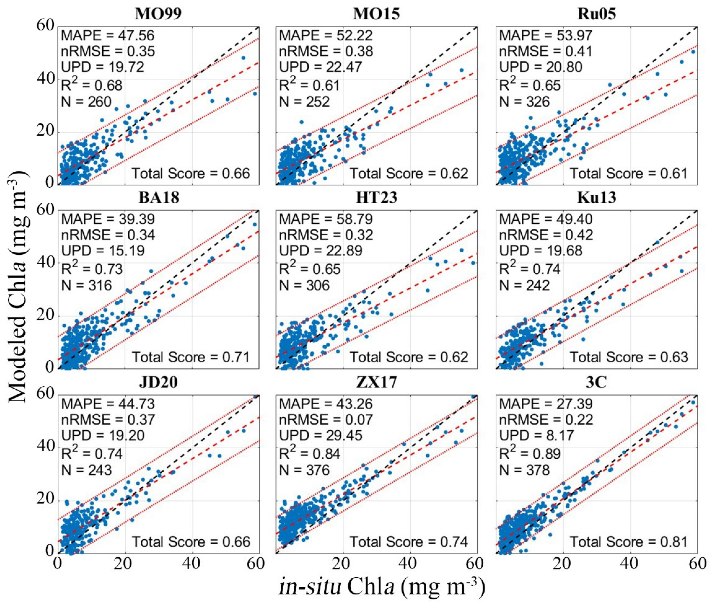
4.1. Parametrization and Validation of Bio-Optical Models

To evaluate the variability of IOPs, the 440 nm normalized IOPs are used to avoid the seasonal variabilities of these parameters (please see Supplement Section S2, Figure S5, and Table S1). Accordingly, the normalized a_Phy(λ) shows low variability (CV = 0.05 at 410 nm and CV = 0.03 at 675 nm), indicating the normalized variability of phytoplankton remains relatively consistent during the measurements. The normalized a_CDOM(λ) shows low values of CV ranging from 0.04 to 0.08 at 410 nm and 675 nm. Similarly, the normalized a_NAP(λ) spectra show a low variability with CV = 0.02 at 410 nm and CV = 0.04 at 675 nm. As a result, the mean values of a*_Phy(λ), a_CDOM(λ₂), a_NAP(λ), S_CDOM, and S_NAP are used for parametrization of the absorption models in Equations (6), (8), and (9) (Table 1). Moreover, the mean values of b*_SPM(λ) = b_SPM(λ)/[SPM] m² g⁻¹ are used for the parametrization of the NAP backscattering coefficient (Equation (12)). Figure 2 shows the correlations between the measured and estimated absorption and backscattering coefficients. The values of MAPE, NRMSE, NBias, MR, and R² of a_Phy(λ) from Equations (6) and (7) against in-situ measurements are 15.0–24.2%, 0.15–0.26, 0.02–0.03, 0.88–0.75, and 0.91–0.84, respectively. The measured a_Phy(λ) spectra exhibit more consistency with the spectra calculated from Equation (6) than Equation (7). The exponential fits of a_CDOM(410) and a_NAP(410) show very good consistency with measurements (MAPE ≤ 3.6%, NRMSE ≤ 0.06, NBias ≤ 0.03, MR ≅ 1.0, and R² ≥ 0.95). The correlation between in-situ a_nw(440) and a_nw,BR19x(440) shows more consistency with measurements than a_nw,LC99(440) (MAPE = 4.3%, NRMSE = 0.11, NBias = 0.04, MR = 0.98, and R² = 0.86). Therefore, parametrization of Equation (3) using a_p,BR18x(λ) (Equation (6) + Equation (8) + Equation (9)) represents the optimum setup that correlates well with the in-situ measurements. Parametrization of b_bp(λ) using b_b,GE05(440) components shows more consistency than those by b_b,BA18(440), with the values of MAPE = 18.8 and 23.8%, NRMSE = 0.12 and 0.16, NBias = 0.03 and 0.04, MR = 0.89 and 0.83, and R² = 0.92 and 0.87, respectively. All estimated IOPs fall within the boundaries of the 95% confidence level of the measurements.

These results confirm that the regional bio-optical models, once parameterized and validated using the HA09 average SIOPs, can reliably simulate spectral IOPs when driven by WCCs (Chla and SPM). This model-based approach provides a physically consistent and validated method to assess glint correction methods under a wide range of environmental conditions.

4.2. Evaluation of ρ and ΔL Estimation Methods

The R_rs,ref(λ) are calculated using Equation (14) utilizing the average of SIOPs (Table 2) and measured WCCs for the time periods when in-situ measurements are available. The R_rs(λ) spectra corresponding to the R_rs,ref(λ) are calculated using the quality-controlled E_d(λ), L_S(λ), and L_T(λ) spectra from south-east and south-west looking sensors spectra in various environmental conditions, based on the proposed methods outlined in Table 3. The eight cases of environmental conditions are considered to cover the main different factors influencing the R_rs(λ) calculation methods (

Table 4. Different environmental conditions are identified for calculating the R_rs(λ). CC = Cloud Cover, WS = Wind Speed (m s⁻¹). The bold underlined items show the key factor in each case.

Case	Title	CC	θS	WS	AOT	Δφ	N
Case I	High Δφ	Clear	θS ≤ 45°	WS ≤ 3	low	Δφ ≥ 60°	65
Case II	Low Δφ	Clear	θS ≤ 45°	WS ≤ 3	low	Δφ ≤ 40°	83
Case III	Overcast skies	Overcasts	45° ≤ θS ≤ 60°	WS ≤ 3	low	40° < Δφ < 60°	115
Case IV	Scattered cloud	Scattered	45° ≤ θS ≤ 60°	WS ≤ 3	low	40° < Δφ < 60°	307
Case V	Extreme WS	Clear	45° ≤ θS ≤ 60°	WS ≥ 9	low	40° ≤ Δφ ≤ 60°	69
Case VI	High WS	Clear	45° ≤ θS ≤ 60°	4 ≤WS ≤ 7	low	40° ≤ Δφ ≤ 60°	211
Case VII	High AOT	Clear	45° ≤ θS ≤ 60°	WS ≤ 3	high	40° ≤ Δφ ≤ 60°	32
Case VIII	High θS	Clear	θS ≥ 80°	WS ≤ 3	low	40° ≤ Δφ ≤ 60°	11

).

Figure 3 shows the average of modeled R_rs(λ) and R_rs,ref(λ) spectra in various environmental conditions. The corresponding error estimates of each case in terms of statistical Total Score (Equation (21)) between R_rs(λ) and R_rs,ref(λ) are shown in Figure 4. The full set of statistical parameters comparing R_rs(λ) and R_rs,ref(λ), and associated scatter plots are shown in the Supplementary Material Figures S6–S9. The results of correlation between R_rs(λ) and R_rs,ref(λ) in different environmental conditions are described below.

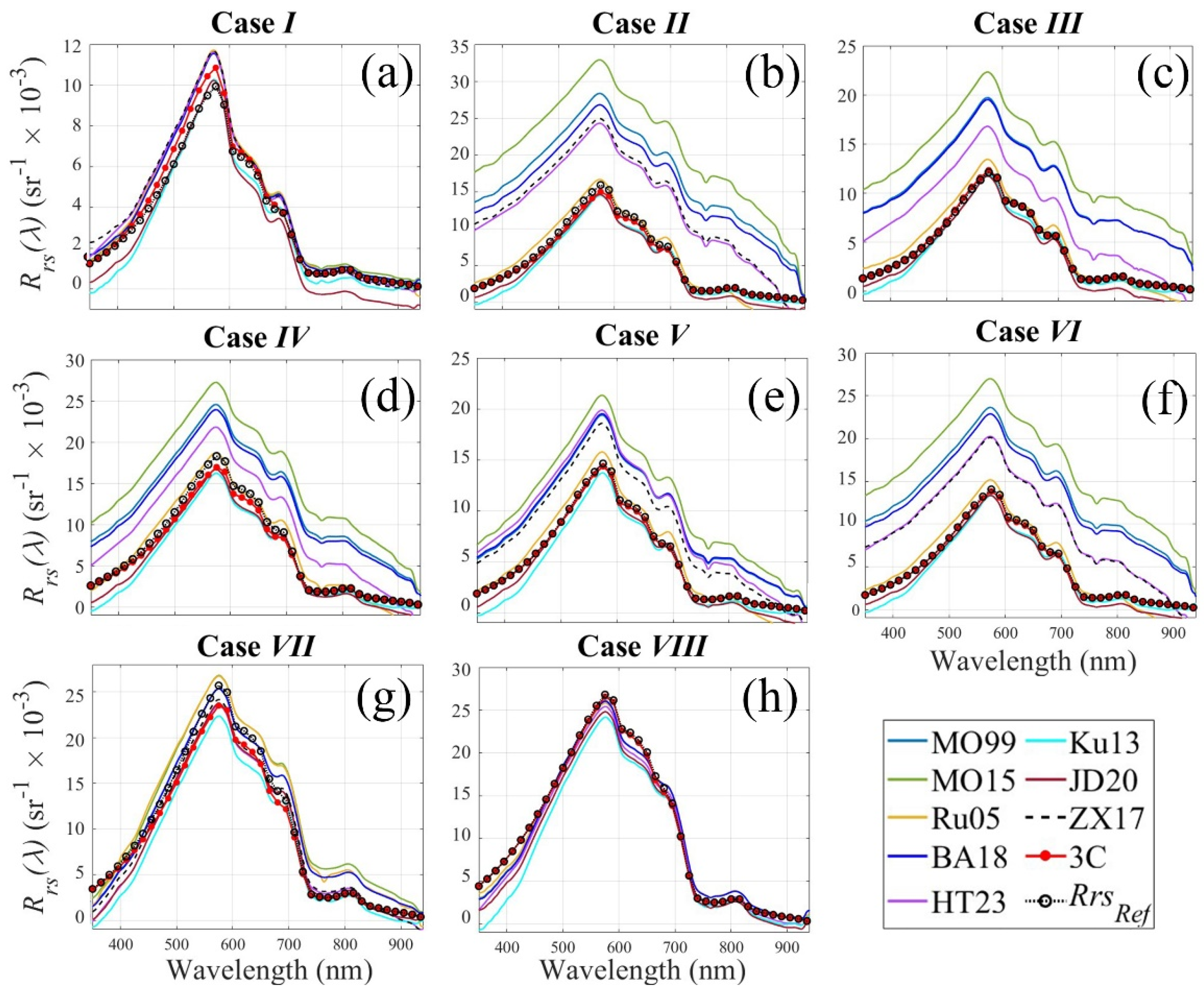
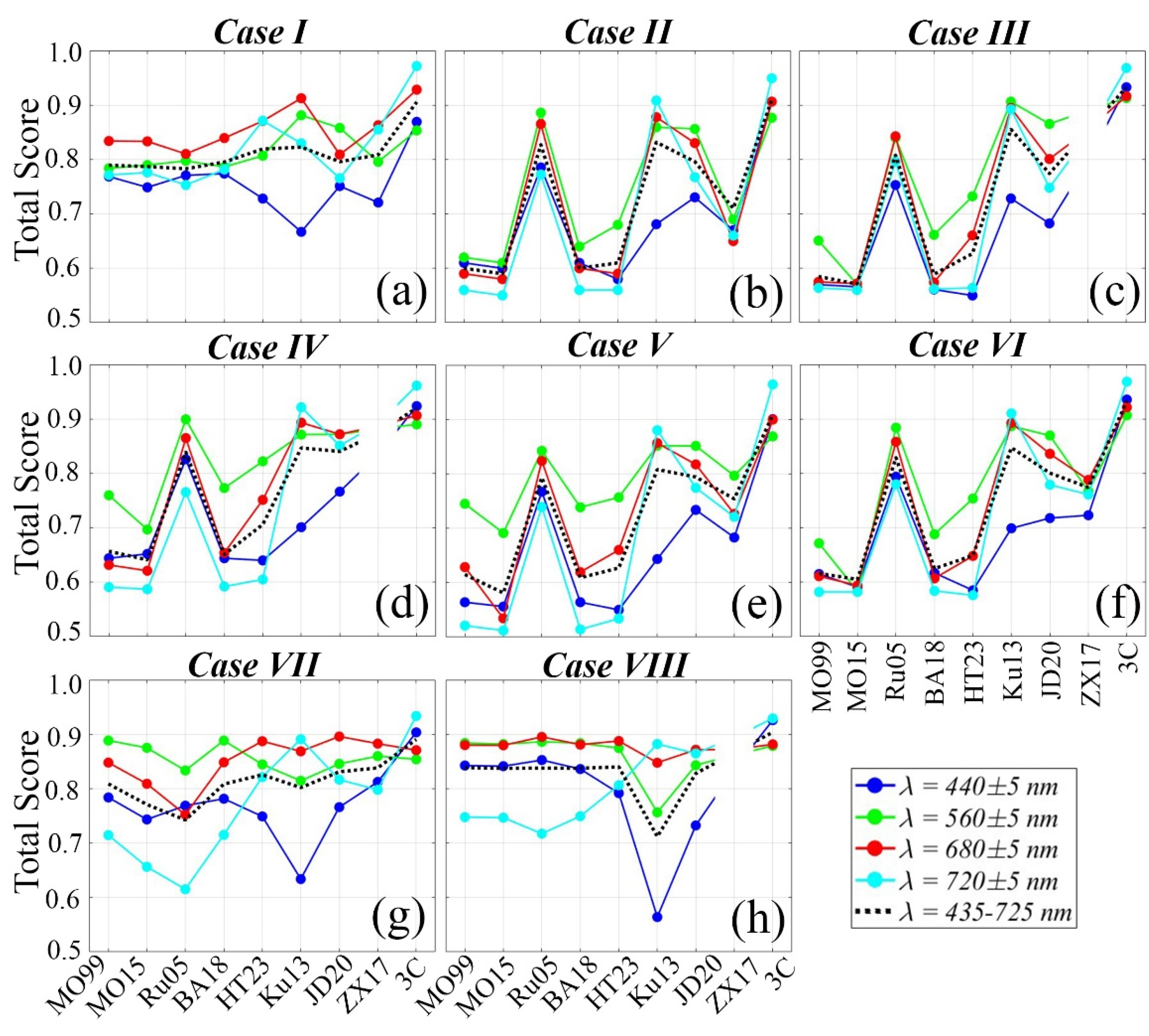
• Case I, High Δφ (Figure 3a and Figure 4a). This case is characterized by low variability of R_rs(λ) spectra. The lowest deviations from R_rs,ref(λ) are achieved by 3C model (Total Score = 0.90, MAPE = 8.8%, UPD = −2.4, NRMSE = 16.1%) in the range of 400–720 ± 5 nm, and the highest deviations by the Ru05 (Total Score = 0.76, MAPE = 32.9%, UPD = −9.7, NRMSE = 24.7%). Similar results are found in the range of λ = 440 ± 5 nm (blue), λ = 560 ± 5 nm (green), λ = 680 ± 5 nm (red), and λ = 720 ± 5 nm (NIR). The other methods show intermediate and relatively similar error estimates against Rrs,ref(λ), with an average of Total Score = 0.79, MAPE = 19–28%, UPD = −8–7, and NRMSE = 24–28%.
• Case II, Low Δφ (Figure 3b and Figure 4b). This case is characterized by high deviations of the models that utilize lookup tables of ρ and BA18. The 3C model shows the best score with Total score = 0.91, MAPE = 8.7%, UPD = 2.9, and NRMSE = 15.8% in the range of 400–720 ± 5 nm. Similar statistical results are observed for the blue, green, red, and NIR regions. The worst statistical scores are observed for MO99, MO15, BA18, HT23, and ZX17 methods with Total Score = 0.56, MAPE > 100%, UPD = −18, and NRMSE = 14–25%.
• Case III, Overcast sky condition (Figure 3c and Figure 4c). The MO99, MO15, BA18, and HT23 show significant overestimations against R_rs,ref(λ) across all wavelengths, with Total Score = 0.54, MAPE = 91–97%, UPD = −14.6–−14.8, NRMSE = 20–24%. The lowest deviation belongs to the 3C model with Total Score = 0.93, MAPE = 7.4%, UPD = 1.5, and NRMSE = 11.8%. The visual comparison shows that the Ku13 and JD20 models significantly underestimate R_rs(λ) in the blue and NIR regions. The ZX17 is not available for this case.
• Case IV, Scattered cloud condition (Figure 3d and Figure 4d). This case is characterized by high deviations and overestimations of MO99, MO15, BA18, and HT23 methods with R_rs(560) = 0.022–0.027 sr⁻¹ and Total Score = 0.59, MAPE = 85–93%, UPD = −12.5–15.2, and NRMSE = 9.1–10.2%. The best simulation belongs to the 3C model with a Total Score of 0.92. The ZX17 is not available for this case.
• Case V, Extreme wind speed (Figure 3e and Figure 4e). Visual comparison of R_rs(λ) spectra indicates the relatively high variability and underestimations in the blue wavelength regions by JD20 and Ku13 methods, which utilize spectral shape for corrections. The 3C and Ru05 show the best performance with Total Score = 0.90 and 0.79, MAPE = 8.8% and 17.3%, UPD = 1.4 and −6.3, and NRMSE = 17.3% and 24.3%, respectively.
• Case VI, High wind speed (Figure 3f and Figure 4f). This case is characterized by overestimation of the MO99, MO15, BA18, HT23, and ZX17 methods with an average of ΔR_rs(560) = 0.009 sr⁻¹ relative to R_rs,ref(λ), with Total Score = 0.58, MAPE = 92–98%, UPD = −16.8–−16.1, and NRMSE = 9.8–11.2%. The 3C model shows the best performance with Total Score = 0.93, MAPE = 6.6%, UPD = 1.2, and NRMSE = 8.8%. The JD20 and Ru05 show the best performance next to the 3C model. The HT23 and ZX17 show similar results.
• Case VII, High AOT (Figure 3g and Figure 4g). This case is characterized by low variability of R_rs(λ) spectra. All models except Ru05 underestimate the R_rs(λ) spectra with an average of ΔR_rs(560) = 0.004 sr⁻¹ relative to the R_rs,ref(λ) spectra in the blue and green regions. The Ku13 and JD20 methods show the highest deviations in the blue and green regions (UPD = 11.5–18.8 and NRMSE = 37.6–60.1%). The HT23 and ZX17 show a good performance in the green-red regions (Total Score = 0.89, MAPE = 9.5%) and a relatively weaker performance in the blue region (Total Score = 0.75, MAPE = 29.3%). Overall, the 3C model shows the best performance, with Total Score = 0.89, MAPE = 9.3%, UPD = 4.6, and NRMSE = 19.1%.
• Case VIII, High sun-zenith angle (Figure 3h and Figure 4h). All methods show low variabilities. Apart from the 3C, the other methods underestimate the R_rs(λ) spectra in the blue-NIR regions. The MO99, MO15, Ru05, BA18, HT23, and JD20 show relatively similar performance with Total Score = 0.81–0.84, MAPE = 11.6–15.1%, UPD = −1.2–4.6, and NRMSE = 30.1–32.4%. The Ku13 shows a very weak performance in the blue region with a Total Score of 0.36. The 3C model shows the best performance in this case with Total Score = 0.92, MAPE = 5.2%, UPD = 0.92, and NRMSE = 22.7%. The ZX17 is not available for this case.

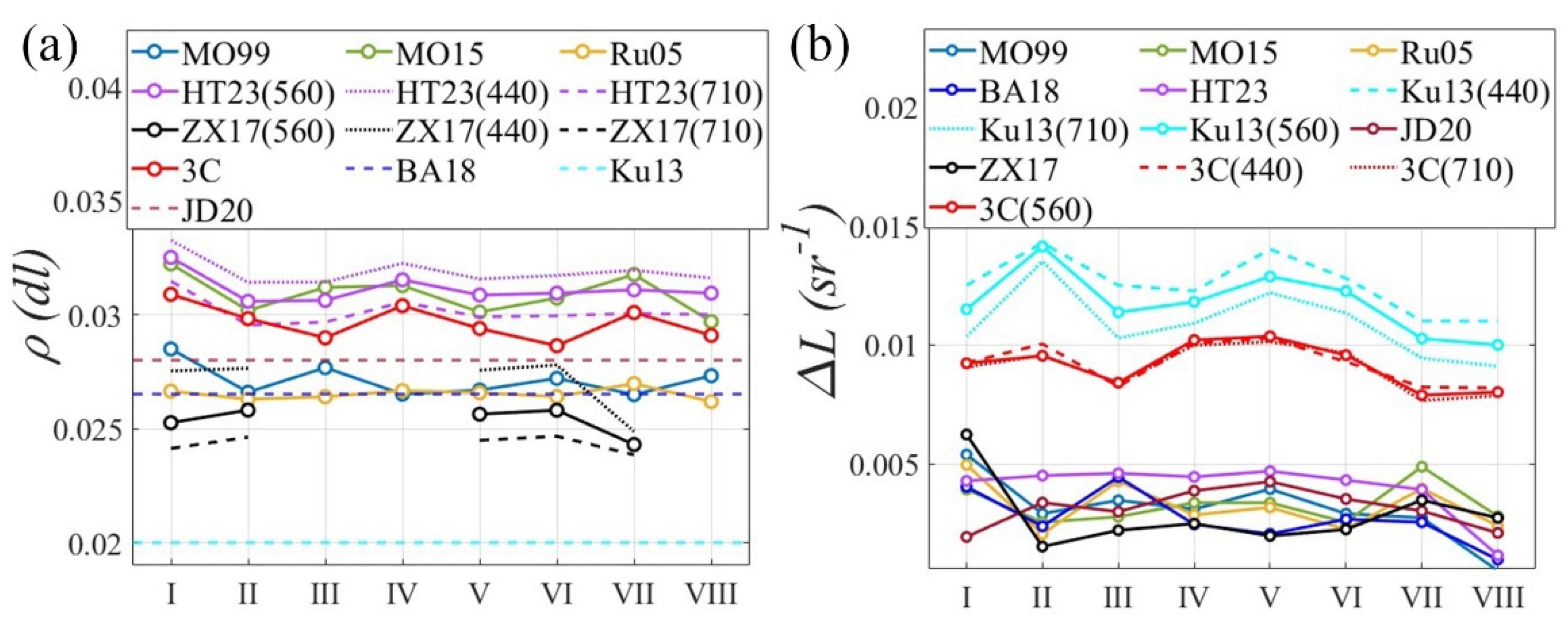
4.3. Variability of ρ and ΔL

Figure 5a shows the variability of ρ values for the eight cases. The ρ values are not highly sensitive to the environmental conditions and are in the range of 0.0271 ± 0.0007 for MO99, 0.0309 ± 0.0008 for MO15, 0.0265 ± 0.0002 for Ru05, 0.03115 ± 0.0006, and 0.0296 ± 0.0008 for 3C. The 3C model exhibits the highest ρ = 0.0308 for Case-I and the lowest value of ρ = 0.0286 for Case-VI. Ku13’s fixed ρ of 0.02 significantly differs from other models. The fixed ρ = 0.0265 of BA18 indicates the minimum value of ρ in various conditions and is very close to the ρ values of Ru05. The Ku13 and JD20 models are not sensitive to the ρ value, as they primarily focus on the reflectance spectral shapes. The HT23 and ZX17 models demonstrate a wavelength-dependent increase in ρ values, decreasing from blue to NIR by an average value of 0.002 in all conditions. While the HT23 and ZX17 have been simulated based on similar environmental conditions (e.g., wind speed and AOT), the ρ(λ) values from these models are significantly different, with averages of ρ(560) = 0.0296 and ρ(560) = 0.0252, respectively.

The models, which result in a wavelength-independent ΔL, exhibit low (≤0.005 sr⁻¹) and relatively uniform ΔL variations in all conditions (Figure 5b). In contrast, the models with wavelength-dependent ΔL (i.e., 3C and Ku13) exhibit higher and more variable ΔL in various conditions. The 3C model shows a wavelength-dependent ΔL with a minimum of 0.0080 sr⁻¹ in Case-VIII and a maximum of 0.0102 sr⁻¹ in Case-IV. The values of 3C-derived ΔL at the blue to NIR regions are very close to the average values (std ≤ 0.001 sr⁻¹) in various conditions. The Ku13 model presents the wavelength-dependent ΔL with the extreme values of 0.0091 sr⁻¹ for Case-VIII and 0.0141 sr⁻¹ for Case-II. The ΔL values of Ku13 decrease from blue to NIR regions by an average of 0.0021 sr⁻¹ in all conditions.

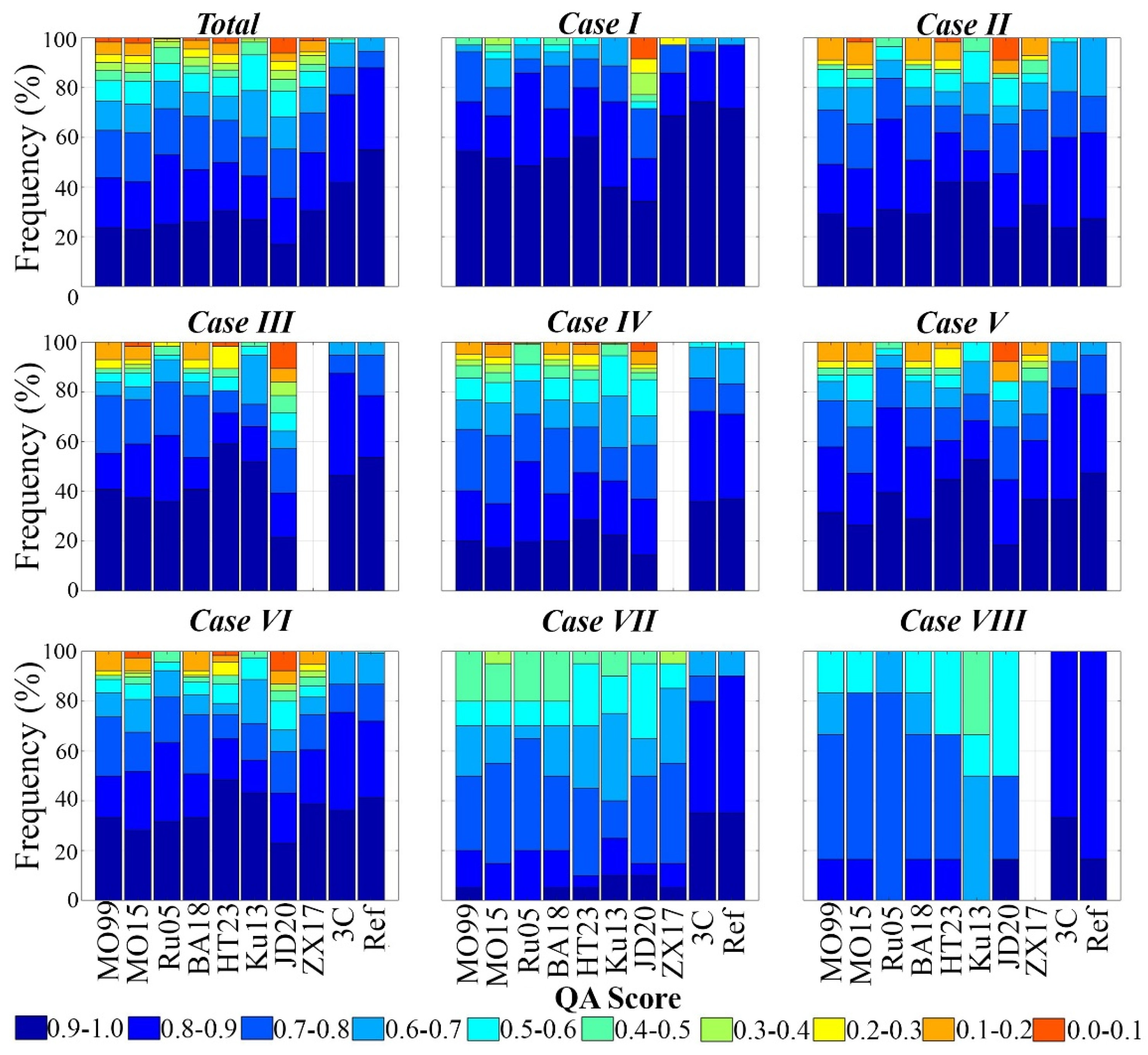
4.4. QA Scores of Simulated Above-Water R_rs(λ)

The threshold of QA ≥ 0.8 was selected to define high-quality R_rs(λ) spectra based on the QA scoring system proposed by [69]. While QA ≥ 0.7 is often used as a general cutoff for usable spectra, our internal tests indicated that a higher threshold of 0.8 offered better consistency with visually and statistically validated reflectance shapes of R_rs,ref(λ) across a wide range of environmental conditions. This threshold thus balances the inclusion of sufficiently high-quality data while minimizing the inclusion of noisy or glint-contaminated spectra.

Figure 6 displays the QA scores for the R_rs,ref(λ) and R_rs(λ) spectra. For the total R_rs,ref(λ) spectra, 55% of spectra achieve QA scores ≥ 0.9, and 88% QA scores ≥ 0.8. The minimum values of QA scores for R_rs,ref(λ) spectra range from 0.6 to 0.7, accounting for 6% of total spectra. The total spectra of the MO99, MO15, and BA18 models show relatively similar QA scores, with an average of 25% of the spectra scoring greater than 0.9 and 24% scoring less than 0.6 (bad/unusable spectra). The total spectra of the JD20 model show the lowest percentage of spectra with a QA score greater than 0.9 (17%) and 23% of bad/unusable spectra (QA ≤ 0.6). Overall, significant portions of the total R_rs(λ) spectra using MO99 (25%), MO15 (27%), Ru05 (18%), BA18 (22%), HT23 (24%), Ku13 (22%), JD20 (32%), and ZX17 (21%) are suspicious or unusable (QA ≤ 0.5). The 3C model shows the best match of R_rs(λ) QA scores with the R_rs,ref(λ) spectra. The total spectra of the 3C model account for 77% of R_rs(λ) with QA scores greater than 0.8, and only 2.3% of spectra have QA scores less than 0.6.

For Case-I, 71% of R_rs,ref(λ), 74% of 3C, and 48–60% of MO99, MO15, Ru05, BA18, HT23, and ZX17 have QA scores ≥ 0.9. The Ku13 and JD20 models have 34% and 40% of spectra with scores ≥ 0.9. About 29% of JD20 spectra are unusable or suspicious (QA ≤ 0.6). The MO15 and BA18 have 9% and 6% of spectra with QA scores ≤ 0.6. For Case-II, III, V, and VI, the R_rs,ref(λ) have QA ≥ 0.7, which shows a relatively similar distribution of QA scores with the 3C model. In these conditions, less than 2% of 3C spectra are unusable/suspicious (QA ≤ 0.6), about 16%-28% of JD20 spectra have QA ≤ 0.6, and about 16–22% of the spectrum from the other models are unusable/suspicious. For Case-IV, less than 3% of R_rs,ref(λ) spectra have a bad QA score. About 30% of JD20 spectra show a bad score, and about 14–22% of the spectrum from the other models have QA ≤ 0.6. The 3C model shows the closest distribution of QA to the R_rs,ref(λ) with only 2.3% of spectra having QA ≤ 0.6. For Case-VII, low percentages of QA scores ≥ 0.9 are observed, with 35% for R_rs,ref(λ) and 3C spectra, and less than 10% for the other models. In this case, more than 30% of all modeled spectra, except 3C, are unusable/suspicious. The lowest percentages of high-quality spectra (QA ≥ 0.9) are observed in Case-VIII, with 17% of R_rs,ref(λ), 33% of 3C, 17% of JD20, and zero for the other models. For Case-VIII, 50% of JD20 and Ku13, 34% of HT23, and 17% of MO99, MO15, and BA18 are bad or suspicious spectra. Overall, the 3C spectra show the highest QA scores, with a distribution similar to that of R_rs,ref(λ), and less than 3% of bad/suspicious spectra under all conditions.

4.5. Showcases of R_rs(λ) Models

Two showcases are presented to illustrate the performance of R_rs(λ) models for Chla and TSM retrieval, respectively. We compare in-situ Chla and TSM with estimated values retrieved from glint-corrected R_rs(λ) based on methods in Table 3. An empirical algorithm developed by NIOZ [12] is used to estimate WCCs from the above-water radiometric measurements. High-quality R_rs(λ) spectra with QA ≥ 0.8 (Section 4.4) are selected for estimation of Chla and TSM. Figure 7 shows the correlations between in-situ and estimated Chla using different methods of R_rs(λ). The R_rs(λ), which utilize lookup tables of viewing direction and winds to estimate ρ (i.e., MO99, MO15, HT23, and Ru05), show relatively similar error statistical metrics, with an average Total Score = 0.63, MAPE = 44%, UPD = 21.5%, NRMSE = 0.36, and R² = 0.65. The ZX17 shows a better performance with Total Score = 0.74 and R2 = 0.84. The methods that utilize a fixed value of ρ (i.e., BA18, Ku13, and JD20) show more consistency with in-situ Chla, with an average Total Score = 0.67, MAPE = 53%, UPD = 18%, NRMSE = 0.37, and R² = 0.73. In contrast, the estimated Chla using the 3C model shows the best results, with Total Score = 0.81, MAPE = 27%, UPD = 8%, NRMSE = 0.22, and R² = 0.89. Figure 8 shows the second showcase of in-situ TSM vs. estimated TSM using different methods of R_rs(λ). The MO99, MO15, Ku13, BA18, and JD20 models show relatively similar results with an average Total Score = 0.69, MAPE = 21%, UPD = 7.8, NRMSE = 0.11, and R² = 0.73. The ZX17 shows a good performance with Total Score = 0.82 and R² = 0.83. The 3C model provides the better performance with MAPE = 15%, UPD = 3.25, NRMSE = 0.09, and R² = 0.79. The 3C model suggests that ~3% of Chla and TSM data falls outside the 95% confidence level, whereas other models indicate ~6–9% of data outside this level. Overall, there is no significant distinction between the models that utilize look-up tables and those that employ fixed ρ values for the estimation of Chla and TSM, with the exception of ZX17, which demonstrates better performance under clear sky conditions.

5. Discussion

Before discussing the findings of this study, we acknowledge two approaches that should be considered in similar studies:

• Sensor Calibration and Algorithm Scope: It is important to note that this study exclusively evaluated above-water glint correction methods using in-situ radiometric measurements and did not involve satellite-based atmospheric correction algorithms. All sensors were maintained and calibrated periodically, with drift monitored through factory servicing and in-field reference checks. Calibration uncertainty was not found to significantly impact the results or the comparative performance of the evaluated glint correction methods. The TRIOS-RAMSES sensors at NJS were subject to periodic factory calibration (every 1–2 years) and routine on-site reference checks using calibrated diffuser panels and lamp standards. Calibration records indicated an annual drift within ±3% for both irradiance and radiance sensors during the study period, remaining within the manufacturer’s specified stability limits. While the primary focus of this study was on above-water glint correction methods, it is acknowledged that calibration drift may contribute to residual errors in retrieved R_rs(λ), particularly under highly dynamic environmental conditions such as monsoon periods. Future work could benefit from integrating explicit calibration drift correction or uncertainty propagation into glint correction assessments.
• Sensor Stability and Thermal Drift Management: The TRIOS-RAMSES radiometers deployed at the NIOZ Jetty Station include internal temperature sensors and manufacturer-provided thermal calibration curves, which automatically correct radiometric data for temperature-induced drift. Temperature metadata were logged during each 10-min measurement and used to monitor operational stability. Periodic factory calibrations were performed, and a comprehensive quality control protocol (based on [36]) was applied to detect and exclude any spectra exhibiting signs of thermal noise, abrupt shifts, or radiometric inconsistencies. Spectra collected during periods of rapid temperature change (e.g., exceeding ±4 °C/h) were flagged and excluded if anomalies were detected in E_d, L_S, or L_T signals. This approach ensured reliable data collection even during diurnal temperature variations exceeding 8 °C.
• Tidal Influence: Although tidal forcing plays a significant role in sediment transport in many estuaries, previous work at the NIOZ Jetty Station [24] demonstrated that tidal phase (ebb vs. flood) had minimal observable effect on diurnal variability of both SPM concentration and above-water radiometric measurements at this site. Consequently, tidal stage was not used as a stratification factor in our glint correction model evaluation. However, in other coastal systems with stronger tidal sediment dynamics, analyzing model performance by tidal phase may offer additional insights.

This study reviews various above-water R_rs(λ) glint-correction methods that use different approaches to estimate ΔL values. We consider the ΔL values of two groups of wavelength-independent and -dependent models, showing a significant difference between the groups (Figure 5b). Our results indicate that the wavelength-dependent ΔL values in the blue to NIR regions are not significantly variable. However, the uncertainties in R_rs(λ) spectra mostly depend on changes in the amplitudes of spectra rather than on the variability of ΔL values [29,77]. In addition, the results confirm the validity of wavelength-independent models for ΔL estimations (Figure 3 and Figure 4). For instance, the presented showcases (Figure 7 and Figure 8) show that the performance of the Ku13 model is relatively similar to the models that use wavelength-independent ΔL estimation (e.g., BA18). It can be inferred that the uncertainty in R_rs(λ) spectra primarily arises from the spectrally dependent shape of the surface-reflected skylight (ρ × L_S(λ)/E_d(λ), second term in Equation (1)) and from accurate estimation of ΔL values, which may be either wavelength-dependent or wavelength-independent. The surface-reflected skylight spectra are highly variable under different sky and surface conditions, particularly at shorter wavelengths (e.g., 350–400 nm) [28]. Therefore, the performance of above-water R_rs(λ) models depends on the simulation of the surface-reflected skylight and accurate estimation of ΔL values.

The presence of aerosols significantly modifies the surface-reflected skylight spectra even for low values of aerosol optical thickness. The HT23 model, which estimates the ρ value as a function of directional factors, surface roughness, and AOT, should be used only under clear-sky conditions [30]. In this study, we estimated the AOT values using inverse modeling of solar downwelling irradiance where no direct measurements of aerosols are available (Section 3.5). It is important to acknowledge that uncertainty in the modeling of AOT affects the results of the HT23 model. However, the HT23 model shows a relatively good performance with a Total Score ≥ 0.8 in clear sky and low wind conditions (Case-I, Case-VII, and Case-VIII) and poor performance (Total Score ≤ 0.6) in roughened surface and cloudy conditions (Figure 4). A more detailed assessment of the HT23 model would involve direct retrieval of aerosols and distinctive measurements [78] or modeling [67,72] of direct and diffusive components of solar downwelling irradiance.

Although 3C is flexible and effective in a variety of environmental and measurement conditions, its performance is inherently tied to the bio-optical model used to simulate the water optical properties. Therefore, its dependency on bio-optical modeling introduces certain limitations and implications for R_rs retrieval. Since the 3C model requires predefined ranges of WCCs and IOPs for SIOP-based L_T/E_d modeling, if the assumed SIOPs do not accurately represent the actual optical properties of the water body, the retrieved R_rs may deviate from the true value. This limitation makes 3C less adaptable to waters with unknown or highly variable optical properties, such as coastal and estuarine waters where IOPs are spatially and temporally dynamic. The impact of this constraint can be significant when trying to retrieve low-magnitude R_rs values in highly turbid or oligotrophic waters (e.g., high solar zenith or low light conditions). This constraint indicates that 3C is not a universal solution for R_rs retrieval but rather an approach that works best in environments where the optical properties are well characterized. Addressing bio-optical constraints through region-specific SIOPs datasets, improved uncertainty quantification, and validation efforts can enhance the robustness of 3C for different aquatic environments.

Moreover, inelastic scattering processes like Chlorophyll-a and CDOM fluorescence contribute significantly to uncertainties in R_rs(λ). Phytoplankton fluorescence at ~685 nm can contribute to a non-negligible fraction of R_rs(λ) that depends on Chlorophyll-a concentration, physiological state, and incident irradiance [79]. CDOM fluorescence at ~400–450 nm further complicates the interpretation of R_rs(λ) [80]. None of the R_rs(λ) glint correction methods (Table 3) account for inelastic scattering, treating it as part of the overall uncertainty. Some bio-optical models include a chlorophyll fluorescence term to correct R_rs(λ) in the 680–690 nm range (e.g., Fluorescence Line Height, FLH) [81]. CDOM fluorescence correction is more challenging, but hyperspectral techniques or fluorescence quantum yield estimates can help. The RT Simulations models, like Hydrolight, for inelastic scattering can be explicitly included in forward simulations to refine R_rs(λ) retrieval algorithms [82]. Given our expertise in this study, incorporating fluorescence into the proposed uncertainty analysis for the 3C might be a valuable next step.

Environmental conditions greatly impact the performance of above-water R_rs(λ) models and contribute to the uncertainty in the corresponding R_rs(λ) spectra. Our findings indicate that the sky cloudiness, solar position, and wind speed are the most important factors affecting fixed above-water radiometry. The above-water R_rs(λ) models are generally less sensitive under clear sky conditions compared to cloudy sky conditions. This is mainly due to smaller variations of ρ and ΔL values in clear sky conditions. Under scattered cloud conditions (Case-IV), models that simulate radiances (i.e., 3C) and account for wind speed to estimate ρ values or models that utilize the spectral shape of R_rs(λ) to estimate ΔL values (i.e., JD20, Ku13) demonstrate good performance (Figure 4). In contrast, the other models that estimate the ρ and ΔL values regardless of cloudiness have poor performance. The MO99, MO15, and HT23 use a lookup table for ρ as a function of wind speed, assuming a Cox-Munk relationship between wind speed and surface roughness [83]. Nevertheless, these models show poor performance (Total Score < 0.6) during windy conditions (Case-V and Case-VI). The BA18, which uses a fixed ρ value, shows poor performance in cloudy and high wind speed conditions. The minimum discrepancies between models during clear sky conditions (Case-I) are observed at θs in the range of 30°–50° and Δφ > 40°. For Δφ ≤ 40°, the 3C, JD23, Ru05, and Ku13 perform relatively better, but it makes sense to omit these spectra. This can be attributed to the impact of the sun’s glint on the surface-reflected skylight, which makes the estimated ρ value from lookup tables invalid for estimating the ΔL values. For θ_S ≥ 80°, all models, with the exception of Ku13, demonstrate strong performance in the range of blue to red wavelengths. However, they exhibit limited effectiveness in the NIR region, with the notable exceptions of the 3C, Ku13, and JD20 models. This indicates that more than 60% of the modeled R_rs(λ) of any model are questionable or unusable, except for the 3C model, which demonstrates robust performance in similar highly turbid waters.

The consistent performance of the 3C model across all environmental conditions may raise concerns about potential overfitting. However, it is important to note that the 3C model is not trained or calibrated on this dataset in the statistical sense. Rather, it is a physically based forward model that uses independent WCC inputs and IOP parameterizations validated in Section 4.1. Its ability to estimate both ρ(λ) and ∆L(λ) dynamically from measurement geometry and atmospheric conditions gives it broader applicability across sky states and surface roughness. In addition, it is worth emphasizing that the 3C model was not tuned to the Chla or TSM concentrations used in the showcase analysis. The forward model used only the glint-corrected R_rs(λ) spectra as inputs to the retrieval algorithm. This further supports that the superior performance of the 3C-corrected spectra in constituent retrieval is not due to overfitting but rather to more accurate glint removal across variable conditions. Meanwhile, the 3C model’s success therefore reflects its structural robustness rather than adaptation to a specific data subset.

This study indicates that the 3C-like methods account for marine environments with multiple scattering effects and varying sky and surface conditions, making the particularly useful in highly turbid waters. However, in estuarine environments where detrital organic matter and SPM significantly contribute to the optical properties, backscattering coefficients vary significantly [84]. This variability could influence the effectiveness of the 3C-like models if not properly parameterized. The 3C model assumes a particular range of backscattering conditions based on empirical data; therefore, modifications may be needed to optimize its performance in estuaries where NAP and resuspended sediments dominate. In addition, the contribution of CDOM is often significant in estuaries [85]. Since CDOM absorption impacts the water-leaving radiance, integrating inelastic scattering effects into the 3C framework could further improve accuracy. Therefore, a wavelength-dependent ρ(λ) on estuarine water conditions might be necessary. Refinements to account for spectral variability in surface reflectance, Chla and CDOM fluorescence, and variable b_bp(λ) contributions will enhance generalizability of 3C-like models across different coastal and estuarine environments.

6. Conclusions

This study reviews and evaluates the well-known bio-optical models and above-water R_rs(λ) glint-correction methods from a fixed automated above-water radiometry under various environmental conditions. The forward modeling of the IOP-to-R_rs transformation using the average of in-situ SIOPs provides a valid fiducial reference for evaluating the above-water R_rs(λ) models from radiometric measurements. Additionally, the performance of R_rs(λ) models, the quality of simulated R_rs(λ) should be considered for practical remote sensing applications. As a general result, the 3C model, which directly simulates the surface-reflected radiance rather than estimating the ρ and ΔL values, provides the best method for modeling R_rs(λ) from automated fixed above-water radiometric hyperspectral measurements during sub-optimal conditions.

References

1. Lee, Z.P. Remote Sensing of Inherent Optical Properties: Fundamentals, Tests of Algorithms, and Applications. In Reports and Monographs of the International Ocean-Colour Coordinating Group (IOCCG); IOCCG: Dartmouth, NS, Canada, 2006. [Google Scholar]
2. Zhang, X.; He, S.; Shabani, A.; Zhai, P.-W.; Du, K. Spectral Sea Surface Reflectance of Skylight. Opt. Express 2017, 25, A1–A13. [Google Scholar] [CrossRef] [PubMed]
3. Steinmetz, F.; Deschamps, P.-Y.; Ramon, D. Atmospheric Correction in Presence of Sun Glint: Application to MERIS. Opt. Express 2011, 19, 9783. [Google Scholar] [CrossRef]
4. Arabi, B.; Salama, M.S.; Wernand, M.R.; Verhoef, W. Remote Sensing of Water Constituent Concentrations Using Time Series of In-Situ Hyperspectral Measurements in the Wadden Sea. Remote Sens. Environ. 2018, 216, 154–170. [Google Scholar] [CrossRef]
5. Alikas, K.; Ansko, I.; Vabson, V.; Ansper, A.; Kangro, K.; Uudeberg, K.; Ligi, M. Consistency of Radiometric Satellite Data over Lakes and Coastal Waters with Local Field Measurements. Remote Sens. 2020, 12, 616. [Google Scholar] [CrossRef]
6. Odermatt, D.; Gitelson, A.; Brando, V.E.; Schaepman, M. Review of Constituent Retrieval in Optically Deep and Complex Waters from Satellite Imagery. Remote Sens. Environ. 2012, 118, 116–126. [Google Scholar] [CrossRef]
7. Kutser, T.; Vahtmäe, E.; Paavel, B.; Kauer, T. Removing Glint Effects from Field Radiometry Data Measured in Optically Complex Coastal and Inland Waters. Remote Sens. Environ. 2013, 133, 85–89. [Google Scholar] [CrossRef]
8. Groetsch, P.M.; Foster, R.; Gilerson, A. Exploring the Limits for Sky and Sun Glint Correction of Hyperspectral Above-Surface Reflectance Observations. Appl. Opt. 2020, 59, 2942–2954. [Google Scholar] [CrossRef]
9. Garaba, S.P.; Schulz, J.; Wernand, M.R.; Zielinski, O. Sunglint Detection for Unmanned and Automated Platforms. Sensors 2012, 12, 12545–12561. [Google Scholar] [CrossRef]
10. Ruddick, K.G.; De Cauwer, V.; Park, Y.-J.; Moore, G. Seaborne Measurements of near Infrared Water-Leaving Reflectance: The Similarity Spectrum for Turbid Waters. Limnol. Oceanogr. 2006, 51, 1167–1179. [Google Scholar] [CrossRef]
11. Wong, J.; Liew, S.C.; Wong, E.; Lee, Z. Modeling the Remote-Sensing Reflectance of Highly Turbid Waters. Appl. Opt. 2019, 58, 2671–2677. [Google Scholar] [CrossRef] [PubMed]
12. Arabi, B.; Salama, M.S.; Wernand, M.R.; Verhoef, W. MOD2SEA: A Coupled Atmosphere-Hydro-Optical Model for the Retrieval of Chlorophyll-a from Remote Sensing Observations in Complex Turbid Waters. Remote Sens. 2016, 8, 722. [Google Scholar] [CrossRef]
13. Luo, Y.; Doxaran, D.; Ruddick, K.; Shen, F.; Gentili, B.; Yan, L.; Huang, H. Saturation of Water Reflectance in Extremely Turbid Media Based on Field Measurements, Satellite Data and Bio-Optical Modelling. Opt. Express 2018, 26, 10435–10451. [Google Scholar] [CrossRef]
14. Mobley, C.D. Estimation of the Remote-Sensing Reflectance from above-Surface Measurements. Appl. Opt. 1999, 38, 7442–7455. [Google Scholar] [CrossRef]
15. Bi, S.; Röttgers, R.; Hieronymi, M. Transfer Model to Determine the Above-Water Remote-Sensing Reflectance from the Underwater Remote-Sensing Ratio. Opt. Express 2023, 31, 10512–10524. [Google Scholar] [CrossRef] [PubMed]
16. Lee, Z.; Ahn, Y.-H.; Mobley, C.; Arnone, R. Removal of Surface-Reflected Light for the Measurement of Remote-Sensing Reflectance from an above-Surface Platform. Opt. Express 2010, 18, 26313–26324. [Google Scholar] [CrossRef]
17. Pitarch, J.; Talone, M.; Zibordi, G.; Groetsch, P. Determination of the Remote-Sensing Reflectance from above-Water Measurements with the “3C Model”: A Further Assessment. Opt. Express 2020, 28, 15885–15906. [Google Scholar] [CrossRef] [PubMed]
18. Werdell, P.J.; McKinna, L.I.W.; Boss, E.; Ackleson, S.G.; Craig, S.E.; Gregg, W.W.; Lee, Z.; Maritorena, S.; Roesler, C.S.; Rousseaux, C.S.; et al. An Overview of Approaches and Challenges for Retrieving Marine Inherent Optical Properties from Ocean Color Remote Sensing. Prog. Oceanogr. 2018, 160, 186–212. [Google Scholar] [CrossRef]
19. Lee, Z.; Pahlevan, N.; Ahn, Y.-H.; Greb, S.; O’Donnell, D. Robust Approach to Directly Measuring Water-Leaving Radiance in the Field. Appl. Opt. 2013, 52, 1693–1701. [Google Scholar] [CrossRef]
20. Gordon, H.R.; Ding, K. Self-shading of In-water Optical Instruments. Limnol. Oceanogr. 1992, 37, 491–500. [Google Scholar] [CrossRef]
21. Doyle, J.P.; Zibordi, G. Optical Propagation within a Three-Dimensional Shadowed Atmosphere–Ocean Field: Application to Large Deployment Structures. Appl. Opt. 2002, 41, 4283–4306. [Google Scholar] [CrossRef]
22. Ruddick, K.G.; Voss, K.; Banks, A.C.; Boss, E.; Castagna, A.; Frouin, R.; Hieronymi, M.; Jamet, C.; Johnson, B.C.; Kuusk, J. A Review of Protocols for Fiducial Reference Measurements of Downwelling Irradiance for the Validation of Satellite Remote Sensing Data over Water. Remote Sens. 2019, 11, 1742. [Google Scholar] [CrossRef] [PubMed]
23. Zibordi, G.; Voss, K.J.; Johnson, B.C.; Mueller, J.L. IOCCG Ocean Optics and Biogeochemistry Protocols for Satellite Ocean Colour Sensor Validation; IOCCG Protocols Series; International Ocean Colour Coordinating Group (IOCCG): Dartmouth, NS, Canada, 2019; Volume 3. [Google Scholar]
24. Zibordi, G.; Hooker, S.B.; Berthon, J.F.; D’Alimonte, D. Autonomous Above-Water Radiance Measurements from an Offshore Platform: A Field Assessment Experiment. J. Atmos. Ocean. Technol. 2002, 19, 808–819. [Google Scholar] [CrossRef]
25. Antoine, D.; d’Ortenzio, F.; Hooker, S.B.; Bécu, G.; Gentili, B.; Tailliez, D.; Scott, A.J. Assessment of Uncertainty in the Ocean Reflectance Determined by Three Satellite Ocean Color Sensors (MERIS, SeaWiFS and MODIS-A) at an Offshore Site in the Mediterranean Sea (BOUSSOLE Project). J. Geophys. Res. 2008, 113, 2007JC004472. [Google Scholar] [CrossRef]
26. Hooker, S.B.; Morrow, J.H.; Matsuoka, A. Apparent Optical Properties of the Canadian Beaufort Sea–Part 2: The 1% and 1 Cm Perspective in Deriving and Validating AOP Data Products. Biogeosciences 2013, 10, 4511–4527. [Google Scholar] [CrossRef]
27. Ruddick, K.; De Cauwer, V.; Van Mol, B. Use of the near Infrared Similarity Reflectance Spectrum for the Quality Control of Remote Sensing Data. In Proceedings of the Remote Sensing of the Coastal Oceanic Environment, SPIE, San Diego, CA, USA, 31 July–1 August 2005; Volume 5885, p. 588501. [Google Scholar]
28. Groetsch, P.M.; Gege, P.; Simis, S.G.; Eleveld, M.A.; Peters, S.W. Validation of a Spectral Correction Procedure for Sun and Sky Reflections in Above-Water Reflectance Measurements. Opt. Express 2017, 25, A742–A761. [Google Scholar] [CrossRef] [PubMed]
29. Jiang, D.; Matsushita, B.; Yang, W. A Simple and Effective Method for Removing Residual Reflected Skylight in Above-Water Remote Sensing Reflectance Measurements. ISPRS J. Photogramm. Remote Sens. 2020, 165, 16–27. [Google Scholar] [CrossRef]
30. Harmel, T. Apparent Surface-to-Sky Radiance Ratio of Natural Waters Including Polarization and Aerosol Effects: Implications for above-Water Radiometry. Front. Remote Sens. 2023, 4, 1307976. [Google Scholar] [CrossRef]
31. Lin, J.; Lee, Z.; Tilstone, G.H.; Liu, X.; Wei, J.; Ondrusek, M.; Groom, S. Revised Spectral Optimization Approach to Remove Surface-Reflected Radiance for the Estimation of Remote-Sensing Reflectance from the above-Water Method. Opt. Express 2023, 31, 22964–22981. [Google Scholar] [CrossRef]
32. Hommersom, A.; Peters, S.; Wernand, M.R.; de Boer, J. Spatial and Temporal Variability in Bio-Optical Properties of the Wadden Sea. Estuar. Coast. Shelf Sci. 2009, 83, 360–370. [Google Scholar] [CrossRef]
33. Mobley, C.D. Polarized Reflectance and Transmittance Properties of Windblown Sea Surfaces. Appl. Opt. 2015, 54, 4828–4849. [Google Scholar] [CrossRef]
34. Arabi, B.; Salama, M.S.; Pitarch, J.; Verhoef, W. Integration of In-Situ and Multi-Sensor Satellite Observations for Long-Term Water Quality Monitoring in Coastal Areas. Remote Sens. Environ. 2020, 239, 111632. [Google Scholar] [CrossRef]
35. Brewin, R.J.W.; Dall’Olmo, G.; Pardo, S.; van Dongen-Vogels, V.; Boss, E.S. Underway Spectrophotometry along the Atlantic Meridional Transect Reveals High Performance in Satellite Chlorophyll Retrievals. Remote Sens. Environ. 2016, 183, 82–97. [Google Scholar] [CrossRef]
36. Choi, J.; Park, Y.J.; Ahn, J.H.; Lim, H.; Eom, J.; Ryu, J. GOCI, the World’s First Geostationary Ocean Color Observation Satellite, for the Monitoring of Temporal Variability in Coastal Water Turbidity. J. Geophys. Res. 2012, 117, 2012JC008046. [Google Scholar] [CrossRef]
37. Qiu, Z. A Simple Optical Model to Estimate Suspended Particulate Matter in Yellow River Estuary. Opt. Express 2013, 21, 27891–27904. [Google Scholar] [CrossRef]
38. Gordon, H.R. A Semianalytic Radiance Model of Ocean Color. J. Geophys. Res. 1988, 93, 10909–10924. [Google Scholar] [CrossRef]
39. Morel, A.; Maritorena, S. Bio-optical Properties of Oceanic Waters: A Reappraisal. J. Geophys. Res. 2001, 106, 7163–7180. [Google Scholar] [CrossRef]
40. Bi, S.; Hieronymi, M.; Röttgers, R. Bio-Geo-Optical Modelling of Natural Waters. Front. Mar. Sci. 2023, 10, 1196352. [Google Scholar] [CrossRef]
41. Moradi, M.; Arabi, B.; Hommersom, A.; van der Molen, J.; Samimi, C. Quality Control Tests for Automated Above-Water Hyperspectral Measurements: Radiative Transfer Assessment. ISPRS J. Photogramm. Remote Sens. 2024, 215, 292–312. [Google Scholar] [CrossRef]
42. Mueller, J.L.; Bidigare, R.R.; Trees, C.; Dore, J.; Karl, D.; Van Heukelem, L. Biogeochemical and Bio-Optical Measurements and Data Analysis Protocols: Ocean Optics Protocols for Satellite Ocean Color Sensor Validation; NASA/TM-2003221621; Goddard Space Flight Space Center: Greenbelt, MD, USA, 2003; Volume 2, pp. 39–64. [Google Scholar]
43. Pegau, W.S.; Gray, D.; Zaneveld, J.R.V. Absorption and Attenuation of Visible and Near-Infrared Light in Water: Dependence on Temperature and Salinity. Appl. Opt. 1997, 36, 6035–6046. [Google Scholar] [CrossRef]
44. Zhang, X.; Hu, L.; He, M.-X. Scattering by Pure Seawater: Effect of Salinity. Opt. Express 2009, 17, 5698–5710. [Google Scholar] [CrossRef]
45. Twardowski, M.S.; Boss, E.; Macdonald, J.B.; Pegau, W.S.; Barnard, A.H.; Zaneveld, J.R.V. A Model for Estimating Bulk Refractive Index from the Optical Backscattering Ratio and the Implications for Understanding Particle Composition in Case I and Case II Waters. J. Geophys. Res. 2001, 106, 14129–14142. [Google Scholar] [CrossRef]
46. Vaillancourt, R.D.; Brown, C.W.; Guillard, R.R.; Balch, W.M. Light Backscattering Properties of Marine Phytoplankton: Relationships to Cell Size, Chemical Composition and Taxonomy. J. Plankton Res. 2004, 26, 191–212. [Google Scholar] [CrossRef]
47. Loisel, H.; Mériaux, X.; Berthon, J.-F.; Poteau, A. Investigation of the Optical Backscattering to Scattering Ratio of Marine Particles in Relation to Their Biogeochemical Composition in the Eastern English Channel and Southern North Sea. Limnol. Oceanogr. 2007, 52, 739–752. [Google Scholar] [CrossRef]
48. Hommersom, A. “Dense Water” and “Fluid Sand” Optical Properties and Methods for Remote Sensing of the Extremely Turbid Wadden Sea; Vrije Universiteit: Amsterdam, The Netherlands, 2010. [Google Scholar]
49. Holm-Hansen, O.; Riemann, B. Chlorophyll a Determination: Improvements in Methodology. Oikos 1978, 30, 438. [Google Scholar] [CrossRef]
50. Mobley, C.D. Radiative Transfer in the Ocean. Encycl. Ocean Sci. 2001, 4, 2321–2330. [Google Scholar]
51. Ogashawara, I.; Li, L.; Druschel, G.K. Retrieval of Inherent Optical Properties from Multiple Aquatic Systems Using a Quasi-Analytical Algorithm for Several Water Types. Remote Sens. Appl. Soc. Environ. 2022, 27, 100807. [Google Scholar] [CrossRef]
52. Bricaud, A.; Babin, M.; Morel, A.; Claustre, H. Variability in the Chlorophyll-specific Absorption Coefficients of Natural Phytoplankton: Analysis and Parameterization. J. Geophys. Res. 1995, 100, 13321–13332. [Google Scholar] [CrossRef]
53. Lee, Z.; Carder, K.L.; Mobley, C.D.; Steward, R.G.; Patch, J.S. Hyperspectral Remote Sensing for Shallow Waters: 2. Deriving Bottom Depths and Water Properties by Optimization. Appl. Opt. 1999, 38, 3831–3843. [Google Scholar] [CrossRef]
54. Bricaud, A.; Morel, A.; Prieur, L. Absorption by Dissolved Organic Matter of the Sea (Yellow Substance) in the UV and Visible Domains. Limnol. Oceanogr. 1981, 26, 43–53. [Google Scholar] [CrossRef]
55. Gege, P. The Water Colour Simulator WASI-User Manual for Version 3. 2005. Available online: https://elib.dlr.de/19338/ (accessed on 20 December 2024).
56. Doxaran, D.; Froidefond, J.-M.; Castaing, P.; Babin, M. Dynamics of the Turbidity Maximum Zone in a Macrotidal Estuary (the Gironde, France): Observations from Field and MODIS Satellite Data. Estuar. Coast. Shelf Sci. 2009, 81, 321–332. [Google Scholar] [CrossRef]
57. Lee, Z.; Carder, K.L.; Mobley, C.D.; Steward, R.G.; Patch, J.S. Hyperspectral Remote Sensing for Shallow Waters. I. A Semianalytical Model. Appl. Opt. 1998, 37, 6329–6338. [Google Scholar] [CrossRef] [PubMed]
58. Petzold, T.J. Volume Scattering Functions for Selected Ocean Waters; Scripps Oceanography: La Jolla, CA, USA, 1972. [Google Scholar]
59. Sathyendranath, S.; Prieur, L.; Morel, A. A Three-Component Model of Ocean Colour and Its Application to Remote Sensing of Phytoplankton Pigments in Coastal Waters. Int. J. Remote Sens. 1989, 10, 1373–1394. [Google Scholar] [CrossRef]
60. Babin, M.; Stramski, D.; Ferrari, G.M.; Claustre, H.; Bricaud, A.; Obolensky, G.; Hoepffner, N. Variations in the Light Absorption Coefficients of Phytoplankton, Nonalgal Particles, and Dissolved Organic Matter in Coastal Waters around Europe. J. Geophys. Res. Ocean. 2003, 108, 3211. [Google Scholar] [CrossRef]
61. Le, C.; Hu, C.; English, D.; Cannizzaro, J.; Chen, Z.; Kovach, C.; Anastasiou, C.J.; Zhao, J.; Carder, K.L. Inherent and Apparent Optical Properties of the Complex Estuarine Waters of Tampa Bay: What Controls Light? Estuar. Coast. Shelf Sci. 2013, 117, 54–69. [Google Scholar] [CrossRef]
62. Lee, Z.; Wei, J.; Voss, K.; Lewis, M.; Bricaud, A.; Huot, Y. Hyperspectral Absorption Coefficient of “Pure” Seawater in the Range of 350–550 Nm Inverted from Remote Sensing Reflectance. Appl. Opt. 2015, 54, 546–558. [Google Scholar] [CrossRef]
63. Pope, R.M.; Fry, E.S. Absorption Spectrum (380–700 Nm) of Pure Water. II. Integrating Cavity Measurements. Appl. Opt. 1997, 36, 8710–8723. [Google Scholar] [CrossRef] [PubMed]
64. Loisel, H. Rrs(0+) -> Rrs(0-) & Water Coefficients. Available online: https://oceancolor.gsfc.nasa.gov/forum/oceancolor/topic_show.pl%3Ftid=2657.html (accessed on 29 July 2024).
65. Lee, Z.; Carder, K.L.; Arnone, R.A. Deriving Inherent Optical Properties from Water Color: A Multiband Quasi-Analytical Algorithm for Optically Deep Waters. Appl. Opt. 2002, 41, 5755–5772. [Google Scholar] [CrossRef]
66. Lee, Z.; Shang, S.; Lin, G.; Chen, J.; Doxaran, D. On the Modeling of Hyperspectral Remote-Sensing Reflectance of High-Sediment-Load Waters in the Visible to Shortwave-Infrared Domain. Appl. Opt. 2016, 55, 1738–1750. [Google Scholar] [CrossRef]
67. Gregg, W.W.; Carder, K.L. A Simple Spectral Solar Irradiance Model for Cloudless Maritime Atmospheres. Limnol. Oceanogr. 1990, 35, 1657–1675. [Google Scholar] [CrossRef]
68. Albert, A.; Mobley, C.D. An Analytical Model for Subsurface Irradiance and Remote Sensing Reflectance in Deep and Shallow Case-2 Waters. Opt. Express 2003, 11, 2873–2890. [Google Scholar] [CrossRef]
69. Wei, J.; Lee, Z.; Shang, S. A System to Measure the Data Quality of Spectral Remote Sensing Reflectance of Aquatic Environments. J. Geophys. Res. Ocean. 2016, 121, 8189–8207. [Google Scholar] [CrossRef]
70. Greene, C.A.; Thirumalai, K.; Kearney, K.A.; Delgado, J.M.; Schwanghart, W.; Wolfenbarger, N.S.; Thyng, K.M.; Gwyther, D.E.; Gardner, A.S.; Blankenship, D.D. The Climate Data Toolbox for MATLAB. Geochem. Geophys. Geosyst. 2019, 20, 3774–3781. [Google Scholar] [CrossRef]
71. Gregg, W.W. A Coupled Ocean-Atmosphere Radiative Model for Global Ocean Biogeochemical Models; National Aeronautics and Space Administration, Goddard Space Flight Center: Greenbelt, MD, USA, 2002. [Google Scholar]
72. Slingo, A. A GCM Parameterization for the Shortwave Radiative Properties of Water Clouds. J. Atmos. Sci. 1989, 46, 1419–1427. [Google Scholar] [CrossRef]
73. Radtran: RADTRAN Solar Irradiance Model with Delta-Eddington Cloud... in Sean-Rohan-NOAA/Trawllight: Derive Apparent Optical Properties from Trawl-Mounted Light Sensors. Available online: https://rdrr.io/github/sean-rohan-NOAA/trawllight/man/radtran.html (accessed on 23 June 2025).
74. Wood, J.; Smyth, T.J.; Estellés, V. Autonomous Marine Hyperspectral Radiometers for Determining Solar Irradiances and Aerosol Optical Properties. Atmos. Meas. Tech. 2017, 10, 1723–1737. [Google Scholar] [CrossRef]
75. Reno, M.J.; Hansen, C.W. Identification of Periods of Clear Sky Irradiance in Time Series of GHI Measurements. Renew. Energy 2016, 90, 520–531. [Google Scholar] [CrossRef]
76. Gupta, H.V.; Kling, H.; Yilmaz, K.K.; Martinez, G.F. Decomposition of the Mean Squared Error and NSE Performance Criteria: Implications for Improving Hydrological Modelling. J. Hydrol. 2009, 377, 80–91. [Google Scholar] [CrossRef]
77. Craig, S.E.; Lohrenz, S.E.; Lee, Z.; Mahoney, K.L.; Kirkpatrick, G.J.; Schofield, O.M.; Steward, R.G. Use of Hyperspectral Remote Sensing Reflectance for Detection and Assessment of the Harmful Alga, Karenia Brevis. Appl. Opt. 2006, 45, 5414–5425. [Google Scholar] [CrossRef]
78. Jordan, T.M.; Simis, S.G.; Grötsch, P.M.; Wood, J. Incorporating a Hyperspectral Direct-Diffuse Pyranometer in an Above-Water Reflectance Algorithm. Remote Sens. 2022, 14, 2491. [Google Scholar] [CrossRef]
79. Gilerson, A.; Zhou, J.; Hlaing, S.; Ioannou, I.; Schalles, J.; Gross, B.; Moshary, F.; Ahmed, S. Fluorescence Component in the Reflectance Spectra from Coastal Waters. Dependence on Water Composition. Opt. Express 2007, 15, 15702–15721. [Google Scholar] [CrossRef]
80. Liu, C.-C.; Miller, R.L. Spectrum Matching Method for Estimating the Chlorophyll- a Concentration, CDOM Ratio, and Backscatter Fraction from Remote Sensing of Ocean Color. Can. J. Remote Sens. 2008, 34, 343–355. [Google Scholar] [CrossRef]
81. Xing, X.-G.; Zhao, D.-Z.; Liu, Y.-G.; Yang, J.-H.; Xiu, P.; Wang, L. An Overview of Remote Sensing of Chlorophyll Fluorescence. Ocean Sci. J. 2007, 42, 49–59. [Google Scholar] [CrossRef]
82. Burkart, A.; Schickling, A.; Mateo, M.P.C.; Wrobel, T.J.; Rossini, M.; Cogliati, S.; Julitta, T.; Rascher, U. A Method for Uncertainty Assessment of Passive Sun-Induced Chlorophyll Fluorescence Retrieval Using an Infrared Reference Light. IEEE Sens. J. 2015, 15, 4603–4611. [Google Scholar] [CrossRef]
83. Cox, C.; Munk, W. Measurement of the Roughness of the Sea Surface from Photographs of the Sun’s Glitter. J. Opt. Soc. Am. 1954, 44, 838–850. [Google Scholar] [CrossRef]
84. Snyder, W.A.; Arnone, R.A.; Davis, C.O.; Goode, W.; Gould, R.W.; Ladner, S.; Lamela, G.; Rhea, W.J.; Stavn, R.; Sydor, M. Optical Scattering and Backscattering by Organic and Inorganic Particulates in US Coastal Waters. Appl. Opt. 2008, 47, 666–677. [Google Scholar] [CrossRef] [PubMed]
85. Lübben, A.; Dellwig, O.; Koch, S.; Beck, M.; Badewien, T.H.; Fischer, S.; Reuter, R. Distributions and Characteristics of Dissolved Organic Matter in Temperate Coastal Waters (Southern North Sea). Ocean Dyn. 2009, 59, 263–275. [Google Scholar] [CrossRef]
Figure 1. (a) Location of NJS and De Kooy meteorological stations. (b) Setup of optical sensors mounted at NJS. 1—ES-UV, 2—Ed, 3—LT south-east, 4—LT south-west, 5—LS south-east, and 6—LS south-west. (c) schematic planar view of sensors. (d) schematic vertical view of sensors.
Remotesensing 17 02209 g001
Figure 2. Correlation between measured and estimated IOPs using the models in Table 1. Black-dashed lines are 1:1, red-dashed lines are linear regression, and dotted-dashed lines are the confidence bounds of 95%. The comparative models are shown as hollow symbols for comparison.
Remotesensing 17 02209 g002
Figure 3. The spectra of Rrs,ref(λ) and the average of modeled Rrs(λ) using various models outlined in Table 3 for different environmental conditions (Case I–Case VIII). The environmental conditions are illustrated in Table 4.
Remotesensing 17 02209 g003
Figure 4. Statistical Total Scores comparing modeled Rrs(λ) with reference Rrs,ref(λ) spectra for eight environmental conditions (Cases I–Case VIII). Case definitions are consistent with Figure 3.
Remotesensing 17 02209 g004
Figure 5. (a) Variations of ρ values obtained from models outlined in Table 3 for different environmental conditions (Case I–Case VIII). (b) similar to (a), but for ΔL values. The environmental conditions are illustrated in Table 4.
Remotesensing 17 02209 g005
Figure 6. Comparisons of QA scores of the modeled Rrs(λ) spectra (N = 918) and Rrs,ref(λ) in various environmental conditions. The environmental conditions are illustrated in Table 4.
Remotesensing 17 02209 g006
Figure 7. Comparison of in-situ and estimated Chla using different models of Rrs. The dotted-red lines and dashed red lines show the statistical confidence level of 95% and the linear trends, respectively. The dashed-black lines show the 1:1.
Remotesensing 17 02209 g007
Figure 8. Comparison of in-situ and estimated TSM using different models of Rrs. Symbols are similar to those in Figure 7.
Remotesensing 17 02209 g008