Abstract
Based on ascending and descending orbit SAR data from 2017–2025, this study analyzes the long time-series deformation monitoring and slip pattern of an active-layer detachment thaw slump, a typical active-layer detachment thaw slump in the permafrost zone of the Qinghai-Tibetan Plateau, by using the small baseline subset InSAR (SBAS-InSAR) technique. In addition, a three-dimensional displacement deformation field was constructed with the help of ascending and descending orbit data fusion technology to reveal the transportation characteristics of the thaw slump. The results show that the thaw slump shows an overall trend of “south to north” movement, and that the cumulative surface deformation is mainly characterized by subsidence, with deformation ranging from −199.5 mm to 55.9 mm. The deformation shows significant spatial heterogeneity, with its magnitudes generally decreasing from the headwall area (southern part) towards the depositional toe (northern part). In addition, the multifactorial driving mechanism of the thaw slump was further explored by combining geological investigation and geotechnical tests. The analysis reveals that the thaw slump’s evolution is primarily driven by temperature, with precipitation acting as a conditional co-factor, its influence being modulated by the slump’s developmental stage and local soil properties. The active layer thickness constitutes the basic geological condition of instability, and its spatial heterogeneity contributes to differential settlement patterns. Freeze–thaw cycles affect the shear strength of soils in the permafrost zone through multiple pathways, and thus trigger the occurrence of thaw slumps. Unlike single sudden landslides in non-permafrost zones, thaw slump is a continuous development process that occurs until the ice content is obviously reduced or disappears in the lower part. This study systematically elucidates the spatiotemporal deformation patterns and driving mechanisms of an active-layer detachment thaw slump by integrating multi-temporal InSAR remote sensing with geological and geotechnical data, offering valuable insights for understanding and monitoring thaw-induced hazards in permafrost regions.
1. Introduction
The Qinghai-Tibetan Plateau (QTP) hosts the largest area of perennial permafrost at low and middle latitudes globally [1], as the permafrost covers approximately 1.06 × 10⁶ km2 [2] and accounts for about 40.32% of the plateau’s total area [3]. The permafrost in this region is characterized as high-altitude, warm (with mean annual ground temperatures (MAGT) often close to 0 °C), and typically ice-rich [4,5]. Over the past five decades, persistent warming, coupled with increasing anthropogenic activities, has led to significant permafrost degradation across the QTP. This degradation is manifested by a reduction in permafrost area, an increase in active layer thickness (ALT), and intensified freeze–thaw cycles [6,7,8]. Permafrost degradation has profound impacts on regional hydrology, ecology, and biogeochemical cycles, including land–atmosphere carbon exchange [9]. In addition, permafrost degradation triggers various thermokarst processes and related geohazards. For instance, thermokarst lakes and ground subsidence commonly develop in flat, ice-rich terrain, whereas thaw slumps and active layer detachments are prevalent on slopes [10,11]. The initiation and retrogressive expansion of thaw slumps expose previously frozen organic matter and ground ice, leading to the accelerated release of greenhouse gases such as CO2 and CH4. This process significantly impacts regional ecosystems [12] and contributes to a positive feedback mechanism that exacerbates global warming [13,14]. Therefore, monitoring and understanding the long-term evolution thaw slumps on the QTP are crucial for developing effective early disaster warning systems and comprehensive risk assessments in this sensitive region.
A thaw slump is a retrogressive landslide feature that develops on slopes underlain by ice-rich permafrost. They initiate when ground ice is exposed, often by natural disturbances or human activities, leading to thawing and subsequent gravitational failure of the overlying thawed soil during the warm season [15]. On the QTP, over 95% of thaw slumps are reportedly initiated by the detachment and sliding of the active layer [15]. These active layer detachments occur when meltwater from thawing ground ice cannot drain efficiently. This leads to increased pore water pressure and a reduction in shear strength at the interface between the thawed active layer and the underlying frozen ground, ultimately triggering failure [16]. Thaw slumps are particularly prone to developing on gentle to moderate slopes (e.g., 3–8°), where conditions favor meltwater pooling above the permafrost table and the accumulation of fine-grained materials [17]. High summer air temperatures and episodes of heavy precipitation are widely recognized as key climatic drivers for the initiation and development of thaw slumps, particularly on such slopes [18,19]. Distinct from the often rapid, singular failure events of landslides in non-permafrost regions, thaw slumps are typically characterized by a more prolonged and progressive development. Once initiated, thaw slump activity can persist and expand retrogressively for years, decades, or even longer, continuing as long as susceptible ice-rich material is exposed and the climatic conditions favor thaw [20]. Overall, the fundamental difference between the two is whether permafrost degradation serves as the primary trigger factor. Given their typically remote locations and prolonged, dynamic evolution, selecting appropriate and effective monitoring methods is crucial for studying thaw slumps in permafrost regions like the QTP.
Interferometric synthetic aperture radar (InSAR) is an advanced satellite remote sensing technique that has become instrumental in the identification and monitoring of various geohazards [21,22,23]. Compared to traditional ground-based geohazard monitoring methods, InSAR technology offers key advantages, including wide-area coverage, high-precision measurements (mm to cm level), and all-weather, day-and-night imaging capabilities [24,25]. While conventional differential InSAR (D-InSAR) is often limited by spatiotemporal decorrelation and atmospheric artifacts [26,27], advanced multi-temporal InSAR techniques such as the SBAS-InSAR method significantly enhance monitoring accuracy and reliability by processing a time series of SAR acquisitions to mitigate these effects and model deformation trends. Particularly for permafrost deformation monitoring, SBAS-InSAR has demonstrated significant utility [28,29]. The SBAS-InSAR technique, which utilizes interferometric pairs with short spatial and temporal baselines, offers several advantages for permafrost monitoring [30,31,32]. First, its inherent design minimizes spatiotemporal decorrelation, making it more robust for monitoring surfaces undergoing seasonal changes and the potentially large deformation gradients that are typical of permafrost environments. Second, by analyzing long time series, SBAS-InSAR can detect slow, millimeter-level deformation, enabling the characterization of gradual processes like thaw-induced subsidence. Third, its ability to provide spatially continuous deformation maps over large areas overcomes the limitations of point-based measurements and is particularly well-suited for remote and often inaccessible permafrost landscapes, as it requires no ground-installed equipment. Consequently, the SBAS-InSAR technique has been increasingly applied to the monitoring of ground deformation in the permafrost regions of the QTP [33,34,35,36]. However, existing SBAS-InSAR applications on the QTP have predominantly focused on regional-scale permafrost stability and thaw subsidence. Detailed investigations into the complex, three-dimensional kinematics and material transport dynamics within individual thaw slumps remains less explored.
This study focuses on a typical active-layer detachment thaw slump located at the northern foot of the Rierlama Mountain of the Qinghai-Tibetan Plateau. Utilizing ascending and descending Sentinel-1A data from 2017 to 2025, this study applied the SBAS-InSAR technique (processed using ENVI5.6.2 and ArcGIS10.8 software) to monitor the long-term surface deformation of the slump and analyze its kinematic patterns. Specifically, the objectives are to (1) quantify the spatiotemporal surface deformation of the thaw slump using SBAS-InSAR time-series analysis; (2) reconstruct the three dimensional displacement field of the thaw slump by integrating ascending and descending orbit SBAS-InSAR results; (3) investigate the driving mechanisms and controlling factors of the thaw slump’s activity by integrating the InSAR-derived deformation with meteorological data (temperature and precipitation), ALT information, and geotechnical properties derived from laboratory tests on soil samples.
2. Study Area and Datasets
2.1. Study Area
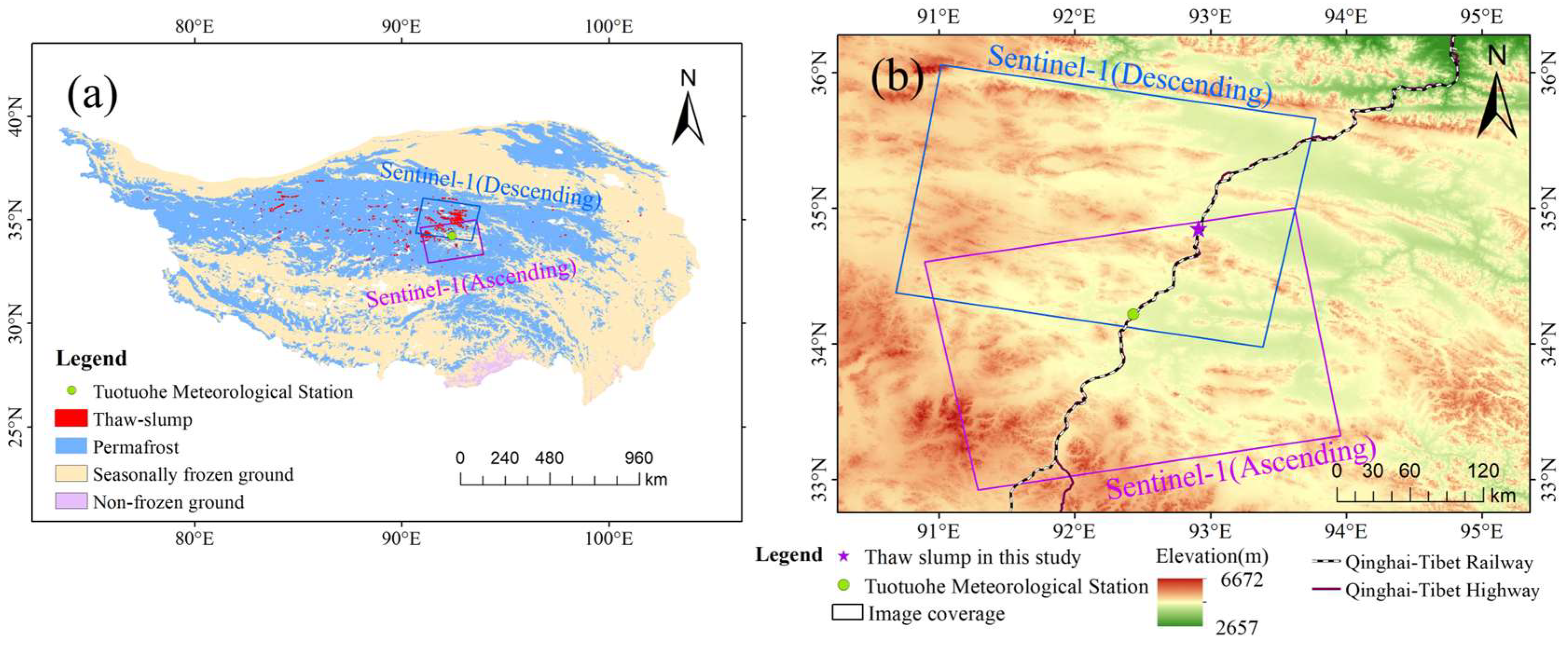
The study area is located in the central region of the QTP (Figure 1a), a region containing critical infrastructure such as the Qinghai-Tibet Highway and Railway (Figure 1b). The specific thaw slump investigated herein is situated near the border of Qinghai Province and the Tibet Autonomous Region. This high-altitude area is characterized by widespread, continuous permafrost and a typical tundra landscape. The regional climate features a mean annual air temperature of approximately −2 °C, with long, cold winters and short, cool summers [37]. The mean annual precipitation ranges from 300 to 400 mm, occurring predominantly during July and August [38]. The thickness of the permafrost layer varies considerably and is significantly influenced by factors such as the temperature and precipitation. The surface vegetation is dominated by alpine meadow, which has an estimated cover of 6–19%. The specific parameters of the thaw slump under investigation are as follows: an area of approximately 4.7 ha, a perimeter of 1.5 km, and an elevation range between 4626 m and 4713 m. The steepest slope of the thaw slump is located at an elevation of about 4713 m. According to Jiao et al. [39], the total disturbed area of this thaw slump is 46,821.3 m2, and the total volume of material displaced by the slide is 81,621 m3. Further investigations suggest that the initial sliding event of the thaw slump occurred around 2016. The thaw slump was selected for study as a typical thaw slump in the permafrost zone of the QTP because of its large scale and relatively recent development.
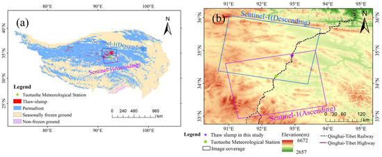
Figure 1.
(a) Location of the study area. Permafrost distribution data for the QTP are from [40], QTP permafrost thaw slump data are from [17]. (b) Elevation data of the study area and the location of the target thaw slump.
2.2. Datasets
2.2.1. Satellite SAR Data and Auxiliary Data
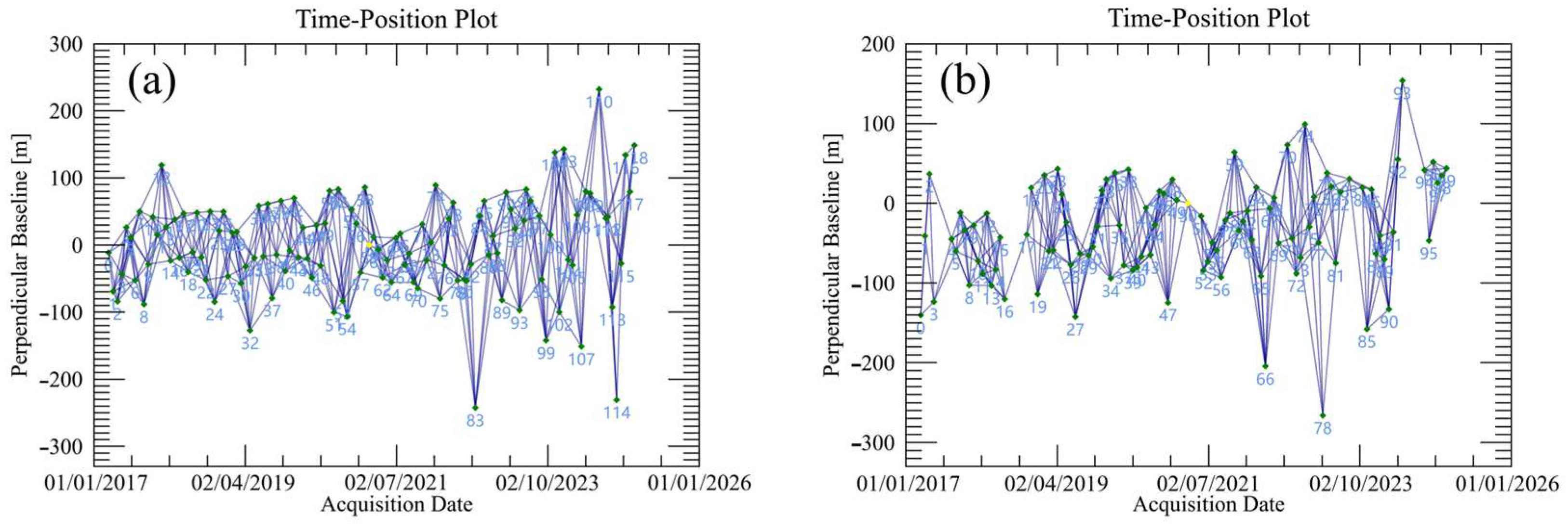
This study utilized C-band Sentinel-1A Single Look Complex (SLC) SAR imagery for deformation monitoring of the target thaw slump. The data were downloaded from the Alaska Satellite Facility (ASF) data portal. A total of 219 Sentinel-1A images were acquired, comprising 119 scenes from ascending orbit and 100 scenes from descending orbit, and spanning the period from 21 March 2017 to 14 January 2025. The spatial coverage of these acquisitions in relation to the study area is shown in Figure 1. Detailed parameters of the Sentinel-1A data used are provided in Table 1. To remove the topographic phase component from the interferograms, a 1 arc-second (approximately 30 m) resolution SRTM DEM was obtained from the United States Geological Survey EarthExplorer portal (https://earthexplorer.usgs.gov/), accessed on 23 September 2014. Precise Orbit Ephemerides data were sourced from the S1QC Hub (https://s1qc.asf.alaska.edu/aux_poeorb/), accessed on 21 March 2017 to 14 January 2025. Figure 2 illustrates the spatiotemporal baseline distribution of the interferometric pairs generated from the selected SAR images for both ascending and descending orbits. The numbers on the connecting lines in the image represent the interferogram numbers.

Table 1.
Parameters of the Sentinel-1A SAR datasets.
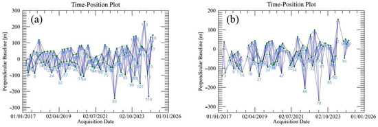
Figure 2.
Spatiotemporal baseline distribution of the selected interferometric pairs for (a) ascending orbit and (b) descending orbit.
2.2.2. Meteorological Data and Active Layer Thickness Data
Meteorological data were sourced from the Tuotuohe meteorological station (latitude: 34.2170°N; longitude: 92.4330°E; elevation 4535 m), which is located approximately 82 km from the study area. The station was selected for its relative proximity and the availability of a consistent long-term record. Daily records of air temperature and precipitation were obtained primarily from the National Cryosphere Desert Data Center (https://www.ncdc.ac.cn/portal/) and supplemented by data from the National Centers for Environmental Information (NCEI) (https://www.ncei.noaa.gov/), accessed on 21 March 2017 to 14 January 2025. Long-term climatic data from this station indicate that January is typically the coldest month, with a mean monthly air temperature of approximately −15 °C, while July is the warmest, with a mean monthly air temperature of around +10 °C. The mean annual precipitation in the region ranges from 300 to 400 mm, with precipitation predominantly occurring during July and August. For contextual information on the active layer thickness (ALT), a dataset was obtained from the National Cryosphere Desert Data Center (https://s.ncdc.ac.cn/portal/metadata/483c1a8f-b73c-41c7-9d9d-406b458f3d39), accessed on 2017 to 2025.
2.2.3. Target Thaw Slump
Field investigations conducted in August 2024 revealed that the thaw slump extends approximately 302–363 m from its headwall to the toe of the main slump body (excluding a secondary mudflow feature on its northwest side), with a maximum width of about 215 m. The headwall is a prominent feature, standing 7–9 m high, with exposures of massive ground ice that are approximately 4–6 m thick visible along its face. The thaw slump is oriented roughly south–north, with material movement predominantly northwards down an average slope of about 8° within the affected area. This slope angle is consistent with previous findings that thaw slumps in permafrost zones commonly occur on gentle slopes [18,41]. Borehole data from an investigation by Jiao et al. [39] in the immediate vicinity of the slump indicate an active layer thickness of approximately 2.5 m. The material near the permafrost table was reported to consist primarily of clay, silty clay, and dense granular material. Beneath the active layer, a thick, ice-rich zone extended from approximately 2.5 m to 6.8 m below the original ground surface; the volumetric ice contents of this zone are estimated at 62–86% [39]. The presence of such thick, ice-rich permafrost provides ideal conditions for thaw slump development. Indeed, field observations in August 2024 confirmed that the thaw slump remains an active feature, continuing to expand. An oblique aerial photograph of the thaw slump, acquired using a DJI Elf 4Pro RTK drone on 12 August 2024, is presented in Figure 3a to illustrate its current morphology and the boundaries used for analysis in this study.
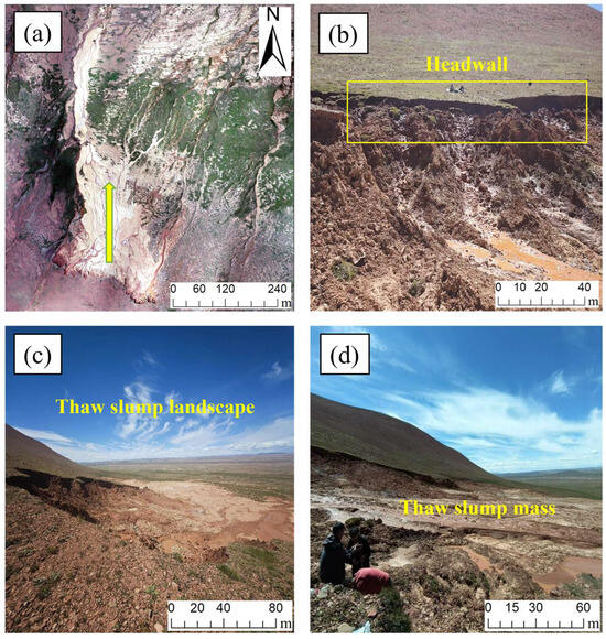
Figure 3.
Morphological characteristics of the thaw slump observed during field investigations in August 2024. (a) Drone aerial image showing the overall extent of the thaw slump; (b) close-up ground view of the active headwall; (c) panoramic ground-level view of the thaw slump; (d) thaw slump mass indicative of mass movement.
3. Methods
3.1. Time-Series InSAR Processing
In this study, the SBAS-InSAR technique, implemented using ENVI SARscape software (version 5.6.2), was employed to monitor surface deformation and analyze the kinematic patterns of the target thaw slump. This version of ENVI SARscape is capable of automatically selecting appropriate ground control points (GCPs) based on the characteristics of the study area. The SBAS-InSAR processing workflow comprised the following key steps for both the ascending and descending Sentinel-1A datasets: 1. Data preparation and co-registration: SLC images were co-registered to a single master scene selected to minimize temporal and perpendicular baseline dispersion for each orbital stack. Precise Orbit Ephemerides were used to refine geometric accuracy. 2. Interferogram generation: Differential interferograms were generated using 30 m resolution SRTM DEM data provided by USGS with phase correction of the terrain in each interferogram [42,43]. 3. Multi-looking and filtering: To reduce speckle noise and improve SNR, interferograms were multi-looked with factors of 1 (azimuth) × 4 (range) for ascending orbit data [44] and 1 (azimuth) × 3 (range) for descending orbit data. The pixel resolution for both the range and azimuth is consistent for both the ascending and descending datasets, with values of 5 m × 20 m for both. During the interferometric processing step, bilinear interpolation is applied to the raw data, resulting in a pixel spacing of 15 m × 15 m after interpolation. A maximum perpendicular (normal) baseline threshold of 5% of the critical baseline and a maximum temporal baseline of 120 days was set. The filtering method employed in this study was Goldstein; 4. Phase unwrapping: Coherence maps were generated for each interferogram. Phase unwrapping was then performed using the minimum cost flow (MCF) algorithm. Given the challenging surface conditions, pixels with coherence below 0.1 were masked out prior to unwrapping; 5. Results interpretation: The final geocoded deformation products covered the period from March 2017 to January 2025. Positive line-of-sight (LOS) deformation values indicate movement towards the satellite, while negative values indicate movement away from the satellite.
We tried the GACOS method to correct for tropospheric delays; however, the results were not satisfactory. We turned to ENVI SARscape’s built-in atmospheric phase screen, which utilizes the SRTM DEM to estimate stratification delays and is suitable for local-scale analyses. However, for future larger-scale studies, we will use GACOS to correct for tropospheric delay effects.
3.2. Three-Dimensional Visualization Solution of InSAR Results
InSAR only measures the surface displacement along the satellite’s line-of-sight (LOS), which is a one-dimensional projection of the true three-dimensional ground deformation vector. To resolve the actual 3D displacement components, typically east–west (E), north–south (N), and up–down (U), it is necessary to combine InSAR measurements acquired from multiple imaging geometries. Resolving the 3D deformation field provides a more comprehensive understanding of surface displacement, offering deeper insights into the kinematics, driving mechanisms, and true extent of geohazards such as landslides and subsidence. To investigate the material transport characteristics and overall kinematic behavior of the thaw slump, this study combines the LOS deformation measurements derived from both ascending and descending Sentinel-1A orbits to reconstruct its 3D displacement field. The methodology for this reconstruction is detailed below.
The LOS displacement measured by InSAR can be expressed as a projection of the 3D displacement vector components—vertical (positive upwards), north–south (positive northwards), and east–west (positive eastwards) (Figure 4)—using the following equations:
where is the radar incidence angle (angle between the LOS vector and the vertical at the target) and is the satellite heading angle (azimuth of the satellite flight path, measured clockwise from north).
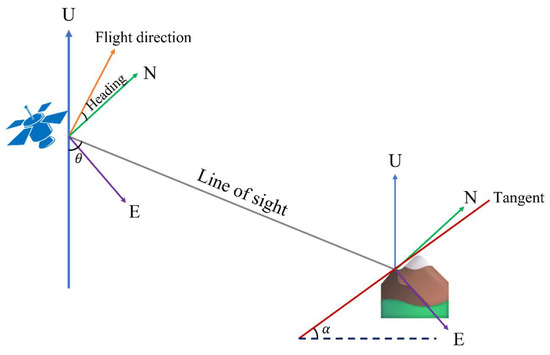
Figure 4.
Schematic illustration of the relationship between the radar LOS direction and the real three-dimensional deformation.
With LOS measurements from different viewing geometries over the same region, a system of equations can be set up to solve for the 3D displacement components:
While assuming negligible north–south displacement can simplify the problem, this component may be significant for features like thaw slumps whose movement direction is strongly controlled by local topography. However, uniquely resolving all three displacement components theoretically requires at least three independent InSAR LOS measurements from different viewing geometries. To address this with only two available LOS geometries (ascending and descending), this study implements a 3D deformation solution by incorporating a physical constraint based on the assumption of surface parallel flow (SPF) [45]. This approach assumes that the thaw slump material moves parallel to the local ground surface. This method leverages a priori information about the local slope gradient and aspect (derived from a DEM) and combines it with the two LOS deformation rate measurements (ascending and descending) to invert the 3D deformation rate components. This approach, suitable for gravity-driven processes like thaw slumps, assumes that the material moves parallel to the local ground surface [46]. The SPF constraint can be written as follows:
where denotes the topographic elevation, and and are the first-order partial derivatives of H with respect to x (easting) and y (northing), respectively. These terms represent the local slope gradients in the east–west and north–south directions and are calculated from the DEM.
By combining the two LOS observations equations and , derived from Equation (2) using Equation (3) and the rearranged SPF constraint (), the system to solve for the 3D deformation rate components can be written in matrix form:
where and are the mean LOS deformation rates from the SBAS analysis of the ascending and descending datasets, respectively.
Based on the above theory, the vertical , north–south , and east–west components of the mean deformation rate were solved. This computation was performed using custom scripts developed in Matlab software R2023a. The resulting 3D deformation rate components were then georeferenced and visualized as maps using ArcGIS 10.8.
3.3. Freeze-Thaw Direct Shear Test
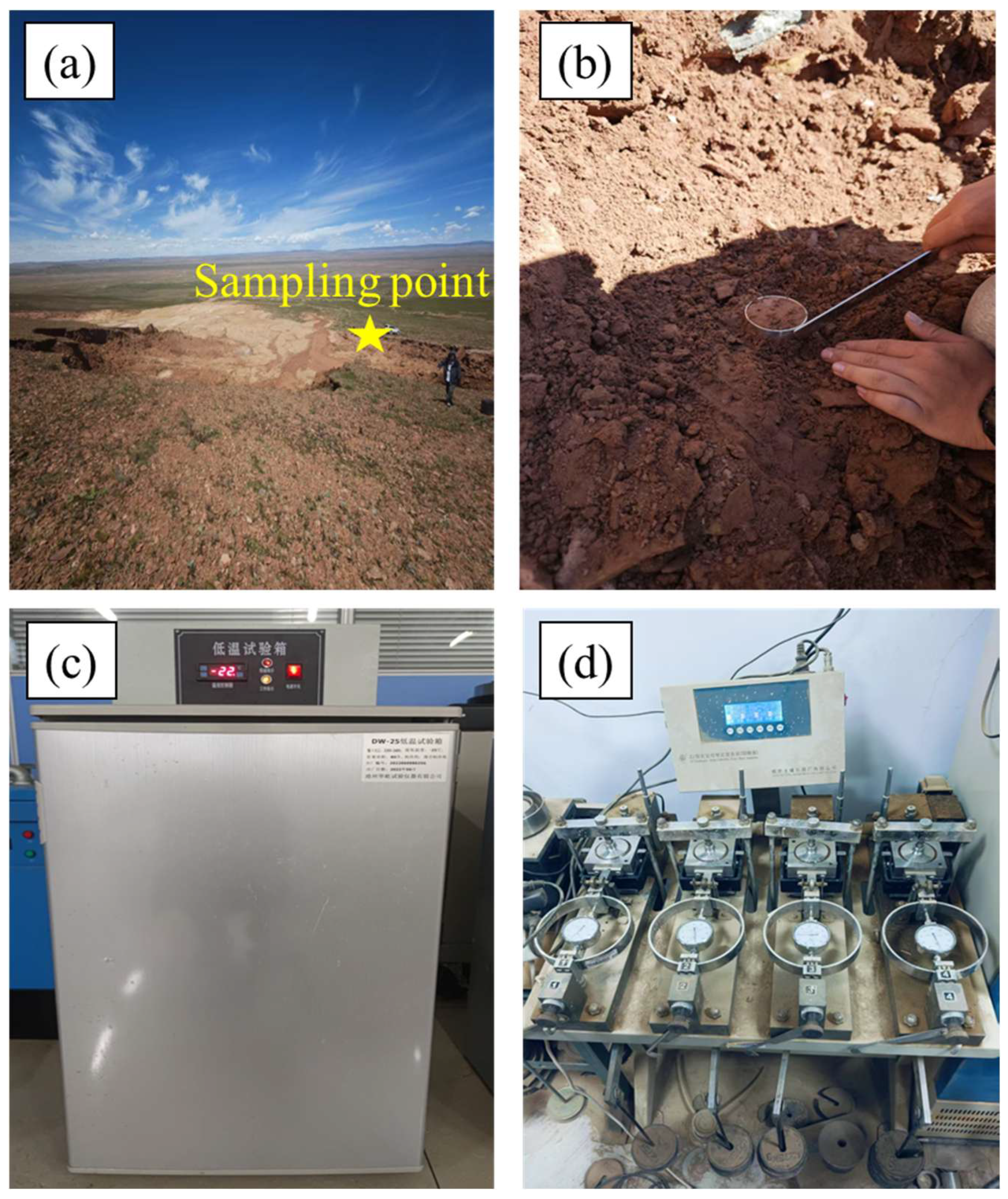
During a field investigation in August 2024, 12 undisturbed soil samples were collected using cutting rings from the relatively undisturbed upper flank of the thaw slump, at a depth of 1.5 m below the surface. Laboratory analysis of these samples yielded an average bulk density of 2.21 g/cm3, a dry density of 1.88 g/cm3, and a natural gravimetric water content of 17.49%. The soil was identified as silty clay. To investigate the impact of freeze–thaw cycles on the soil shear strength, a series of direct shear tests were performed. For this, soil samples were remolded to a gravimetric water content of 20% to ensure homogeneity and consistent initial conditions. For each of the six freeze–thaw cycle counts (0, 1, 3, 5, 10, and 15 cycles), direct shear tests were conducted under four distinct normal stresses, with triple samples being taken for each stress, totaling 72 samples for the cyclic freeze–thaw investigation. Each freeze–thaw cycle consisted of 12 h of freezing at temperatures from −25 °C to −20 °C followed by 12 h of thawing at 20 °C~25 °C. These temperature settings and durations were chosen based on regional temperature data and previous laboratory studies on permafrost soil mechanics [47,48]. The freeze–thaw tests were carried out in a low-temperature test chamber. Following each cycle count, samples were allowed to thaw completely at room temperature (15 °C) for 24 h before being subjected to direct shear testing. The direct shear instrument used was the “ZJ-type strain-controlled direct shear instrument (quadruple shear)” manufactured by Nanjing Soil Instrument Factory (Figure 5), with a constant shear rate of 1.2 mm/min.

Figure 5.
Soil sampling and laboratory equipment for freeze–thaw direct shear testing. (a) Location of the soil sampling point. (b) An undisturbed soil sample collected in a cutting ring. (c) Freeze–thaw test chamber. (d) The ZJ-type strain-controlled quadruple direct shear apparatus used for determining the shear strength parameters.
This section quantifies the effect of freeze–thaw cycling on the shear strength of permafrost soils through freeze–thaw direct shear tests, which provide a mechanistic explanation of thaw slump deformation mechanisms. The aim is to verify whether freeze–thaw cycling contributes to the occurrence and development of thaw slumps by decreasing soil stability through mechanisms such as breaking intergranular bonding and increasing the pore water pressure. InSAR data, such as line-of-sight (LOS) deformation rates and 3D displacement fields, reveal the phenomenon of surface deformation in thaw slumps, while freeze–thaw experiments explain the underlying mechanical causes of the deformation, which allows the establishment of complementary “phenomenon-mechanism” relationships.
4. Results
4.1. Thaw Slump Deformation Rate
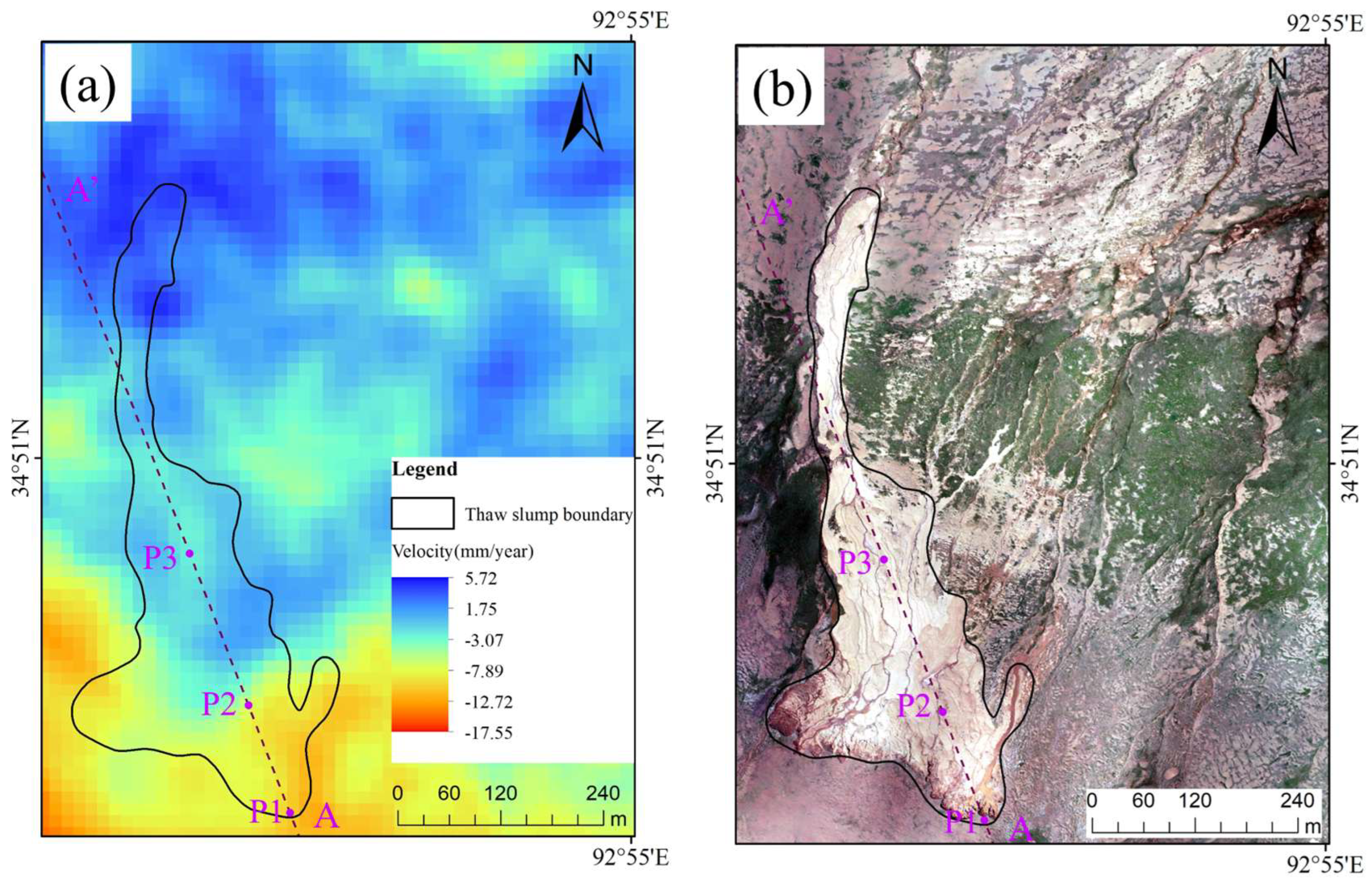
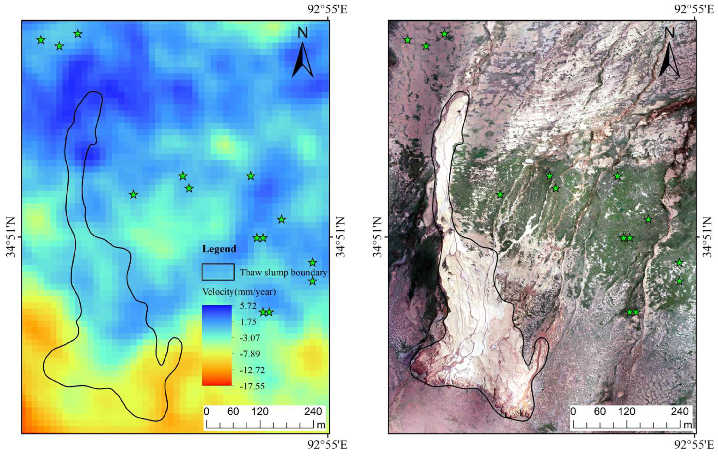
The SBAS-InSAR processing of Sentinel-1A data from March 2017 to January 2025 yielded time-series surface deformation results for the thaw slump and its immediate surroundings. A total of 5402 coherent measurement points were identified within the study area. Figure 6 presents a map of the mean LOS deformation rates for these points, geocoded to a pixel spacing of 15 m × 15 m. Negative deformation rates (colored red) indicate movement away from the satellite’s LOS, which is often associated with subsidence or material deflation within the thaw slump. Conversely, positive deformation rates (colored blue) indicate movement towards the satellite’s LOS. The magnitude of the deformation rate is represented by the intensity of the color, with larger absolute values indicating higher rates of surface movement. Regarding the reference (undeformed) points, we denote them using “asterisks” in Figure 7.

Figure 6.
LOS deformation rates and visual context for the thaw slump. (a) Mean annual LOS deformation rates (mm/year) of thaw slump. The locations of profile line AA′ (purple dashed line) and characteristic points P1, P2, and P3 (purple dots) are overlaid. (b) Oblique aerial photograph of the thaw slump acquired by drone in August 2024.

Figure 7.
Position of the reference (undeformed) points. “Asterisks” represent reference (undeformed) points.
To further analyze the spatiotemporal patterns of deformation, a profile line AA’ was drawn across the main axis of the thaw slump, and three characteristic points, P1, P2, and P3, along this profile were selected for detailed quantitative analysis (Figure 6). The mean LOS deformation rates observed within the thaw slump area range from approximately −17.55 mm/year to +5.72 mm/year, exhibiting significant spatial heterogeneity. Spatially, the highest rates of negative LOS deformation (movement away from the satellite) are concentrated in the southern/upper part of the thaw slump, which encompasses the headwall and main source area. Point P1, located in this zone, exhibits a mean LOS deformation rate of −17.55 mm/year, which is indicative of significant subsidence and material evacuation. Moving downslope along the profile, point P2 shows a rate of approximately −8.33 mm/year, and point P3 records a rate of approximately −2.27 mm/year. This gradient of LOS deformation rates reflects the spatial variability within the slump body, which is likely influenced by factors such as differential thaw, variations in ground ice content, and soil properties. Overall, the LOS deformation within the delineated thaw slump boundary is predominantly negative, which is consistent with the observed net subsidence and downslope material transport. However, the deformation of most areas outside the boundary is relatively small. The magnitude of these negative LOS deformation rates generally decreases from the primary source area (near P1) to the more distal parts of the slump (P2, P3).
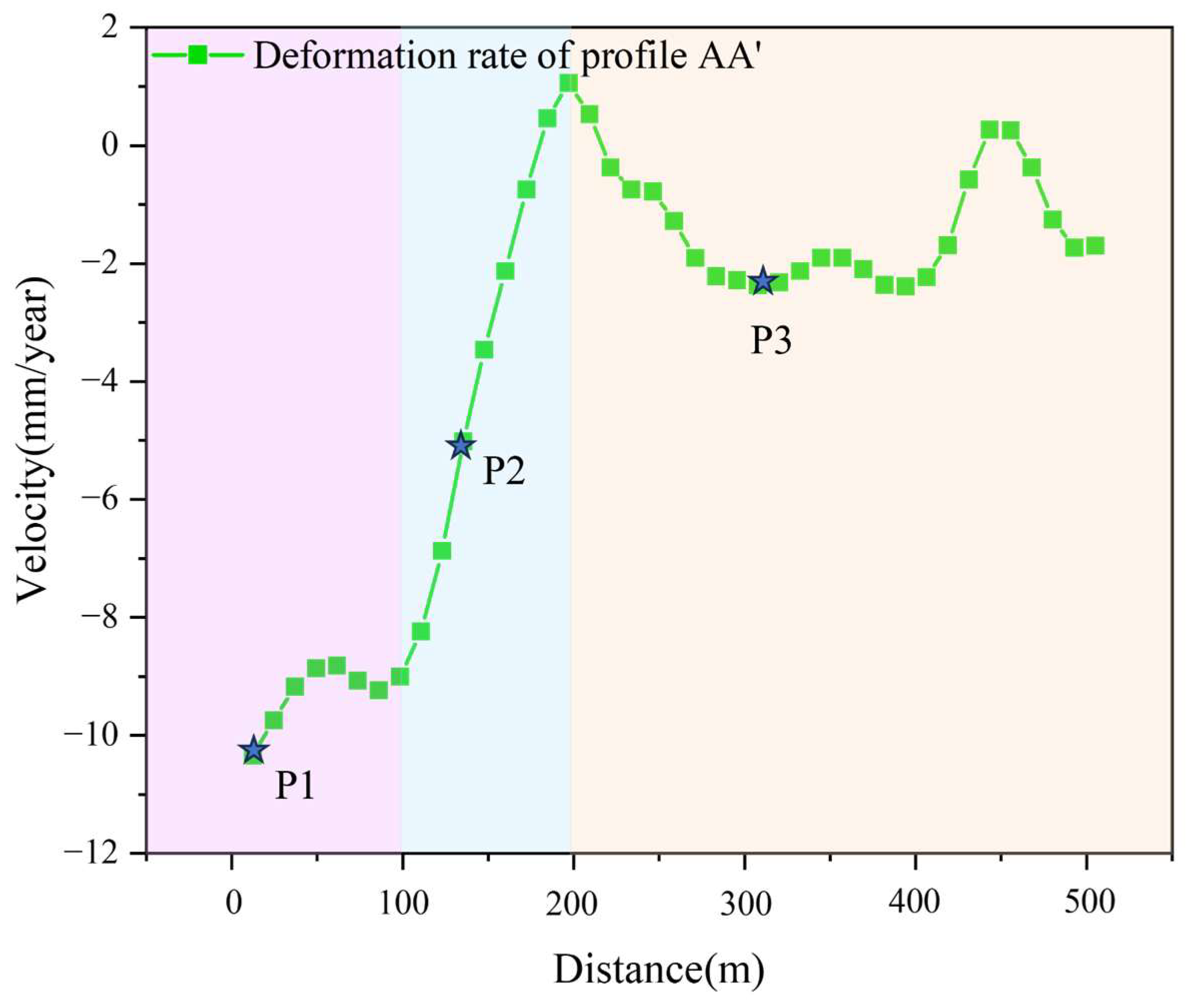
Quantitative analysis of the LOS deformation rates along profile line AA’ (Figure 8), which extends from the headwall (0 m) downslope through the main body of the thaw slump, reveals the spatial variation pattern of its movement. The deformation rate profile shows that the initial 0–100 m segment (corresponding to the primary source area) exhibits significant negative LOS deformation, with rates that average approximately −10 mm/year. Between 100 m and 200 m along the profile, the magnitude of the negative LOS deformation rate progressively decreases, indicating continued but less intense movement away from the satellite. Around the 200 m mark, the deformation rates approach 0 mm/year, suggesting a transition zone towards relative stability. Further along the profile, from 200 m to 490 m (approaching the slump toe), the LOS deformation rates fluctuate between −2 and 0 mm/year, indicating slight residual subsidence or downslope creep in this section. Overall, the LOS deformation rate profile demonstrates a general trend of maximum negative deformation (subsidence) in the upper source area, and gradually transitions to near-stable conditions or minor residual movement towards the distal part of the slump. Significant differences in the deformation rates along the profile highlight the spatial non-uniformity of the movement within the thaw slump.
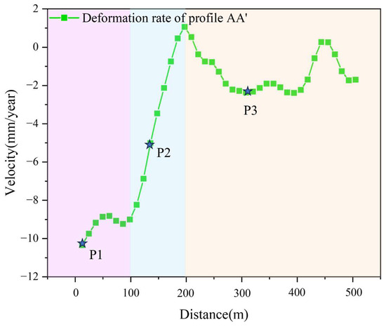
Figure 8.
Profile of mean annual LOS deformation rates (mm/year) along transect AA′ (location shown in Figure 6a).
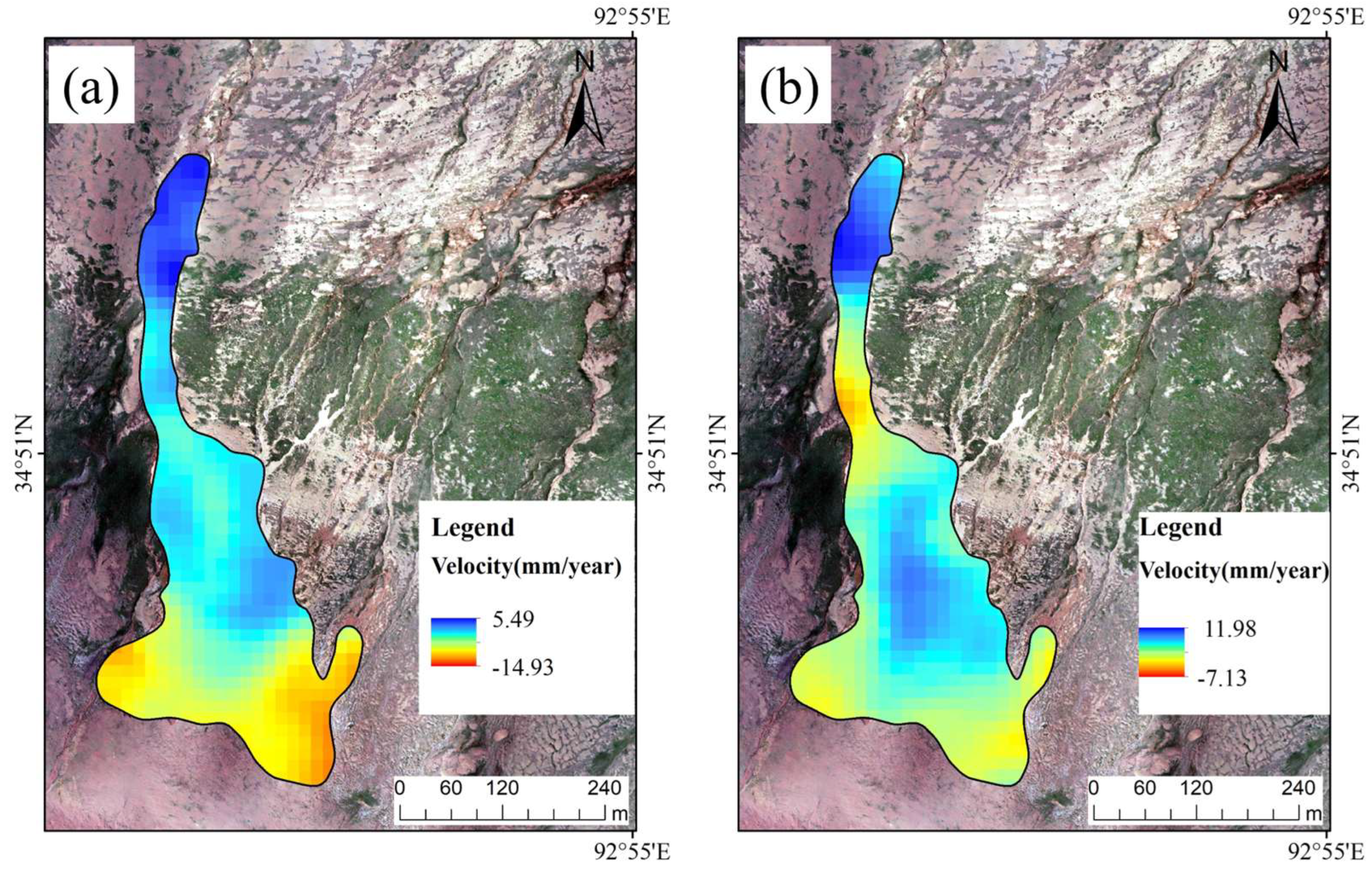
Ideally, ground GNSS receivers should be used to validate the results. However, as we know, deploying GNSS measurements in the remote and inaccessible permafrost regions of the QTP presents significant challenges. To address this, we employed multiple reliability checks: the ascending and descending data show relatively consistent deformation patterns in terms of a “south-to-north” sliding trend in the deformation rates and headwall subsidence and toe accumulation in the thaw slump (Figure 9); and the highest deformation rate (−17.55 mm/year) aligns with field observations, which is a known area of thaw slump damage. In addition, according to the TLS-UAV joint detection results of Jiao et al. (2023) [39], the first active layer detachment of the thaw slump occurred before 2016, accompanied by the rapid melting of thick underground ice (ice content of 62~86%) at the back wall, which formed a steep bank with a height of 5.2~7.5 m. The survey conducted by Luo et al. [15] of the river basin at the northern foot of the QTP revealed that the thaw slump in this area entered an active period due to exceptionally high temperatures during 2015–2016, and subsequently transitioned into a slow evolution stage dominated by creep. Since the SAR data of this study begin in March 2017, this study did not capture the severe deformation in 2016, but only recorded the creep deformation from 2017 to 2025. Nevertheless, the deformation field interpreted by InSAR is consistent with their field results: the deformation at the headwall of the thaw slump is the largest and subsiding, and the toe of the thaw slump exhibits accumulation; the deformation intensity of the thaw slump decreases from the headwall to the toe (e.g., the settlement rate from P1 to P3 decreases from −17.55 mm/year to −2.27 mm/year). This is consistent with the “exponential decay of thermal perturbation with distance” pattern obtained from the numerical simulation by Jiao et al. [39] and verifies the “source-sink” material transport mode of the thaw slump.
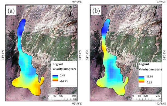
Figure 9.
Comparison of the mean annual deformation rate (mm/year) of LOS in ascending and descending orbits. (a) Ascending orbit LOS deformation rate; (b) descending orbit LOS deformation rate.
4.2. SBAS-InSAR Deformation Time-Series Analysis
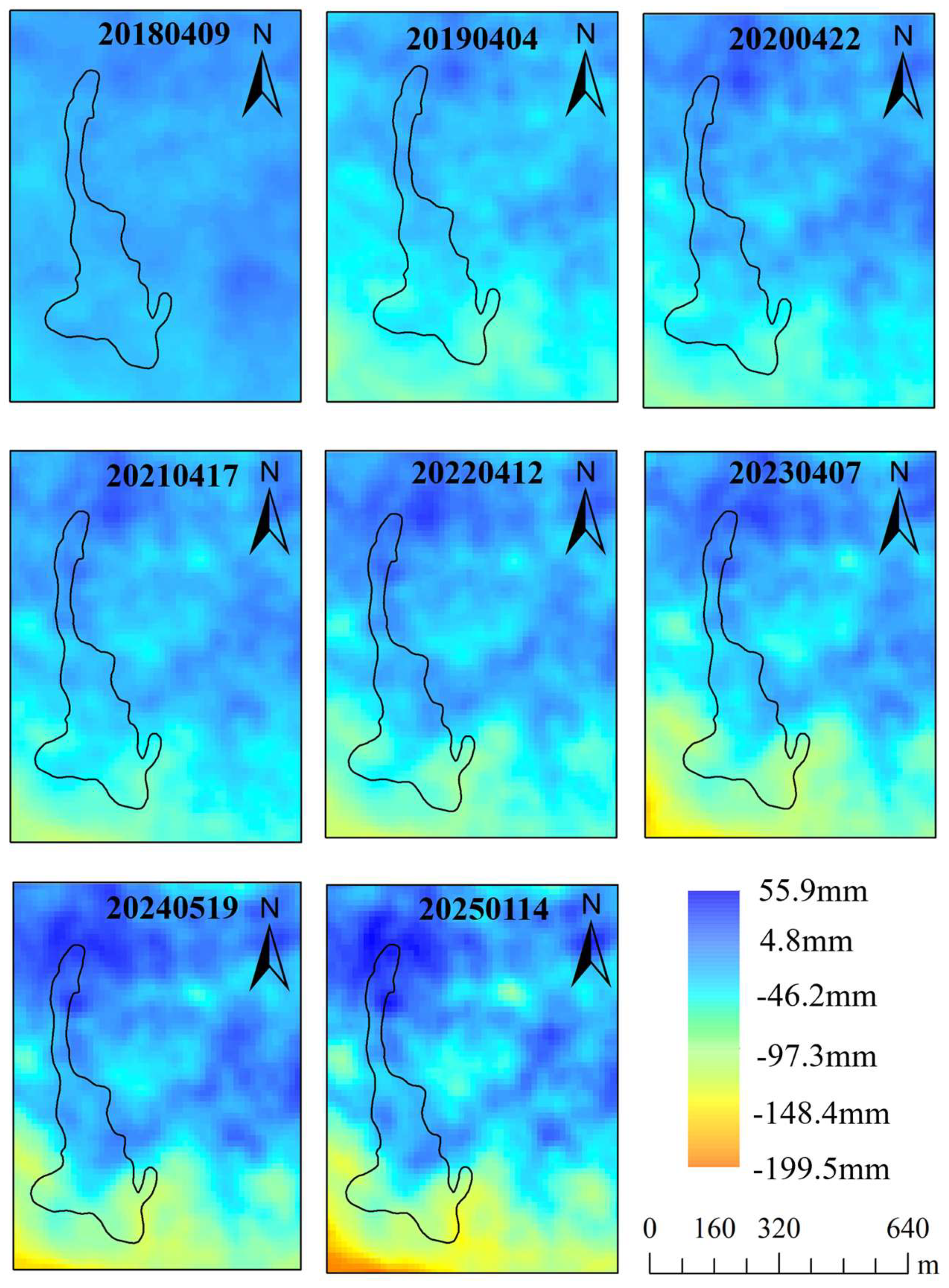
The SBAS-InSAR technique was used to derive cumulative LOS deformation time series for the target thaw slump from March 2017 to January 2025. Figure 10 presents these time series for the characteristic points P1, P2, and P3, previously identified in Figure 6a. The cumulative LOS displacements across the entire thaw slump during the observation period range from approximately −199.5 mm to +55.9 mm. Within the delineated thaw slump boundary, the deformation is predominantly negative, indicating that most of this area experienced net movement away from the satellite, which is consistent with subsidence and material deflation/evacuation. Analysis of the time-series plots reveals the temporal evolution of the deformation at these specific locations. The subsidence in the lower part of the region (south of the thaw slump) is the most significant. Overall, the SBAS-InSAR time series demonstrates persistent activity and complex spatiotemporal dynamics within the thaw slump throughout the observation period. This highlights the ongoing instability of this feature, which will be further analyzed in conjunction with meteorological data to understand its drivers and relationship with freeze–thaw cycles.
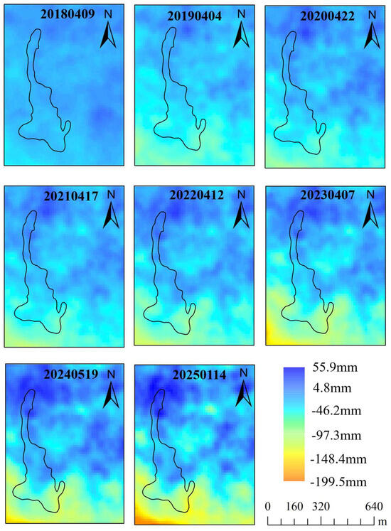
Figure 10.
Map of cumulative displacement (mm) of the target thaw slump from 9 April 2018 to 14 January 2025. The black line in the figure indicates the thaw slump boundary, delineated from UAV aerial imagery acquired in August 2024.
Figure 11 resents the time-series curves of the millimeter-scale deformation at the three characteristic points (P1, P2 and P3) within the thaw slump area. Point P1, located in the headwall/source area, exhibits a continuous negative trend, with its cumulative displacement reaching approximately −80 mm. This represents the largest and most consistent subsidence among the three points. This indicates that P1 is situated in an area that is significantly affected by thaw slump activity, where permafrost thaw likely leads to continuous soil instability and prominent cumulative subsidence. Point P2, located in the mid-slump area, shows an overall negative trend, with its cumulative displacement reaching approximately −60 mm. Point P3, situated in the lower/distal part of the slump, remained relatively stable around 0 mm of displacement, after which it exhibited minor negative displacement. This indicates that P3 was less affected by the thaw slump activity, potentially due to its location near the slump toe or underlying soil with lower ice content or more stable mechanical properties. In summary, the significant and persistent subsidence at P1 and P2 confirms their location within the active source and transport zones of the thaw slump, where the permafrost thaw-induced soil deformation is more intense. In contrast, P3 shows a more subdued and potentially lagging deformation response, which likely reflects differences in its location relative to the main slump activity or variations in local ground conditions.
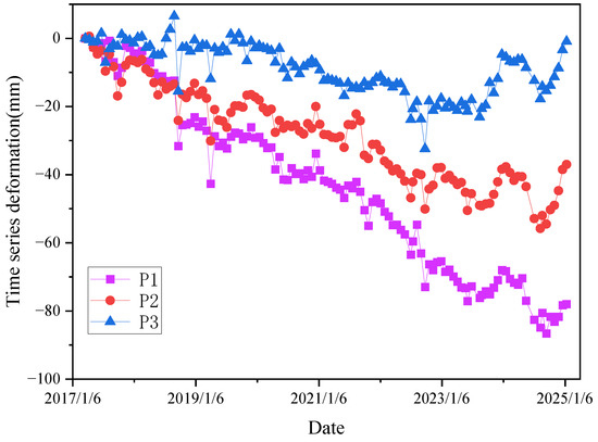
Figure 11.
Time series of cumulative displacement (mm) at characteristic points P1, P2, and P3.
4.3. Three-Dimensional Visualization of Thaw Slump Deformation Analysis
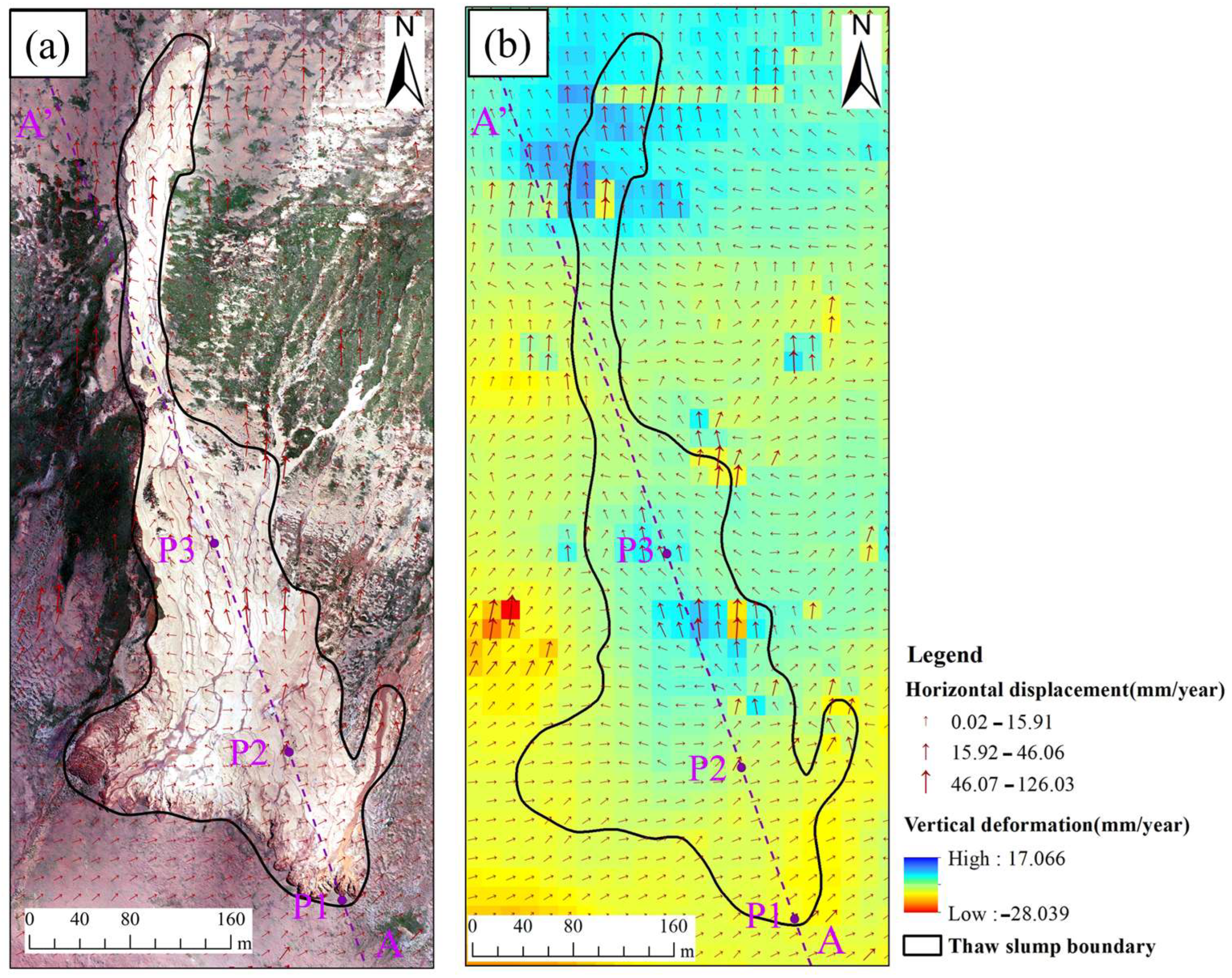
Figure 12 presents the 3D deformation field of the target thaw slump, which was derived by combining ascending and descending orbit InSAR data with the surface parallel flow constraint. The magnitude of the vertical displacement components is represented by the color scale. The magnitude of the total horizontal displacement is indicated by the length of the arrows, and the direction of horizontal movement is shown by the arrow orientation. Analysis of the 3D deformation field reveals the following key kinematic characteristics of the thaw slump.
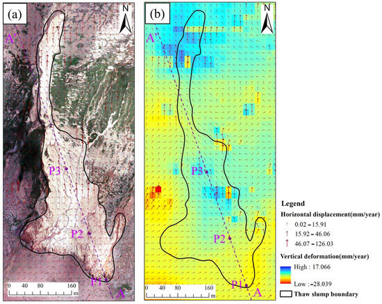
Figure 12.
Three-dimensional deformation field of the thaw slump. (a) Aerial image map of the field. (b) Map of the 3D deformation rates.
The thaw slump exhibits an elongated morphology with a heterogeneous distribution of 3D deformation rates within its boundaries. The northernmost part of the thaw slump (toe region, depicted in blue-green hues) exhibits the highest positive vertical deformation rates, reaching up to approximately +17.07 mm/year. This significant uplift is interpreted as material accumulation and stabilization at the slump toe. The areas depicted in yellow tones, primarily in transitional zones, show relatively small vertical deformation rates (close to 0 mm/year). In contrast, the regions that are colored red, concentrated in the upper/southern source area, experience significant subsidence, with vertical deformation rates reaching −28.04 mm/year. Overall, the vertical deformation field within the thaw slump is highly non-uniform, with patchy areas of both positive and negative vertical deformation being observed near the delineated slump boundaries, which suggests complex localized processes. The arrows indicating horizontal displacement are generally longer within the slump boundary compared to those within the surrounding stable terrain. Particularly, significant horizontal deformation rates are observed in the central transport zone of the slump, roughly between points P2 and P3. The direction of horizontal displacement is predominantly from south to north, aligning with the overall downslope orientation and movement direction of the thaw slump. The observed 3D deformation field, characterized by substantial subsidence in the source area, significant downslope horizontal transport, and accumulation at the toe, illustrates the typical mass wasting process of an active thaw slump. After permafrost thawing, the degree of consolidation of the soil decreases, which generates both vertical subsidence (or uplift) and drives horizontal sliding under the influence of gravity. The minimal 3D deformation observed in the terrain immediately outside the delineated slump boundary further underscores that the pronounced ground instability is primarily localized within the active thaw slump feature.
Furthermore, the 3D deformation field (Figure 12b) reveals a zone of significant horizontal deformation (indicated by relatively long arrows) located immediately west of the main thaw slump boundary, adjacent to the P2–P3 segment. This area, while outside the currently delineated primary slump, exhibits notable ongoing horizontal movement. This indicates substantial instability and a propensity for sliding in this adjacent zone. Corroborating these InSAR findings, optical imagery of this specific western zone (Figure 12a) reveals distinctive compressional features on the ground surface, such as soil folds or pressure ridges. These morphological features are consistent with the effects of sustained horizontal compressive stress, likely resulting from material movement and squeezing when space is restricted or inter-particle forces are unbalanced. The combination of the measured horizontal displacement and the observed compressional surface features strongly suggests that the ground in this adjacent area is destabilized. Based on these observations, we hypothesize that the thaw slump has the potential for future lateral expansion into this western adjacent zone.
4.4. Freeze-Thaw Shear Test
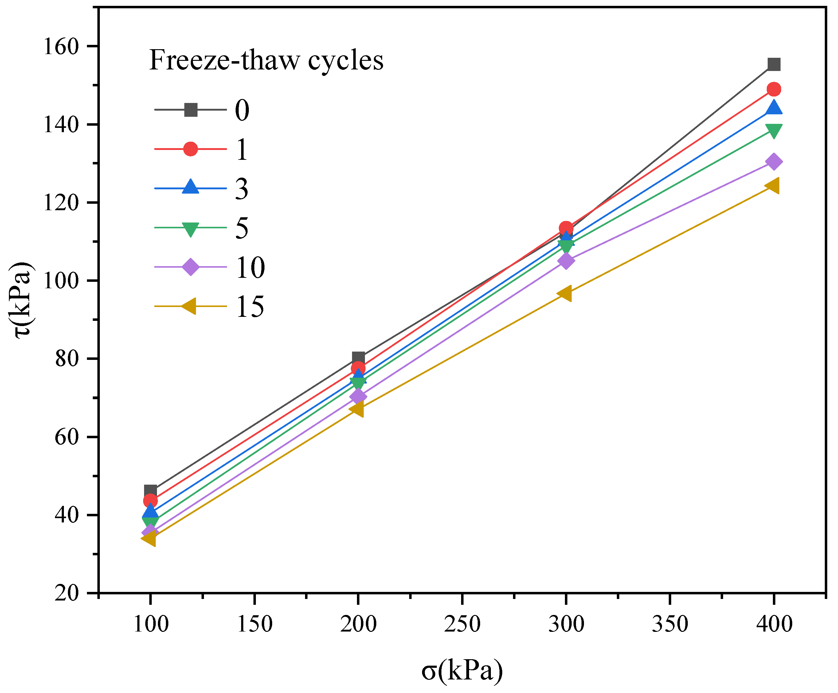
In Figure 13, the horizontal axis represents the vertical pressure σ(kPa), and the vertical axis represents the peak shear stress τ(kPa). The results of direct shear tests, conducted on remolded soil samples subjected to varying numbers of freeze–thaw cycles, clearly demonstrate that repeated freezing and thawing significantly degrades the soil shear strength (Figure 13). Specifically, for any given applied normal stress, the peak shear stress sustained by the soil samples at failure decreased as the number of freeze–thaw cycles increased. The failure envelope derived from the samples subjected to 15 freeze–thaw cycles was significantly lower than that for the uncycled (0 freeze–thaw cycles) samples across the entire range of tested normal stresses. This confirms that freeze–thaw cycling progressively damages the internal soil structure. As the number of freeze–thaw cycles increased, the cumulative damage to the soil fabric intensified, leading to a more pronounced deterioration of the shear strength. According to Table 2, it is evident that the effective cohesion of the soil samples shows a significant decrease with an increasing number of freeze–thaw cycles. Similarly, the effective internal friction angle also exhibited a decreasing trend with an increasing number of freeze–thaw cycles.
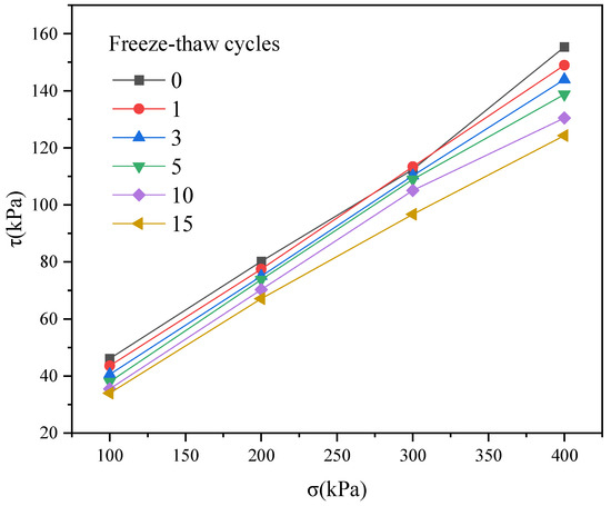
Figure 13.
Damage trajectory for the soil samples in σ − τ space.
Table 2.
Shear strength parameters of soil samples under different numbers of freeze–thaw cycles.
5. Discussion
While extreme precipitation events are often the primary trigger for landslides in many non-permafrost environments [49], the development and activity of thaw slumps in permafrost regions are governed by a more complex interplay of factors. In these cryotic environments, variables including rising air and ground temperatures, precipitation patterns (both rain and snow), the active layer thickness (ALT), the soil ice content, and the mechanical effects of freeze–thaw cycles all exert significant, often interacting, influences on thaw slump initiation and evolution.
5.1. Temperature
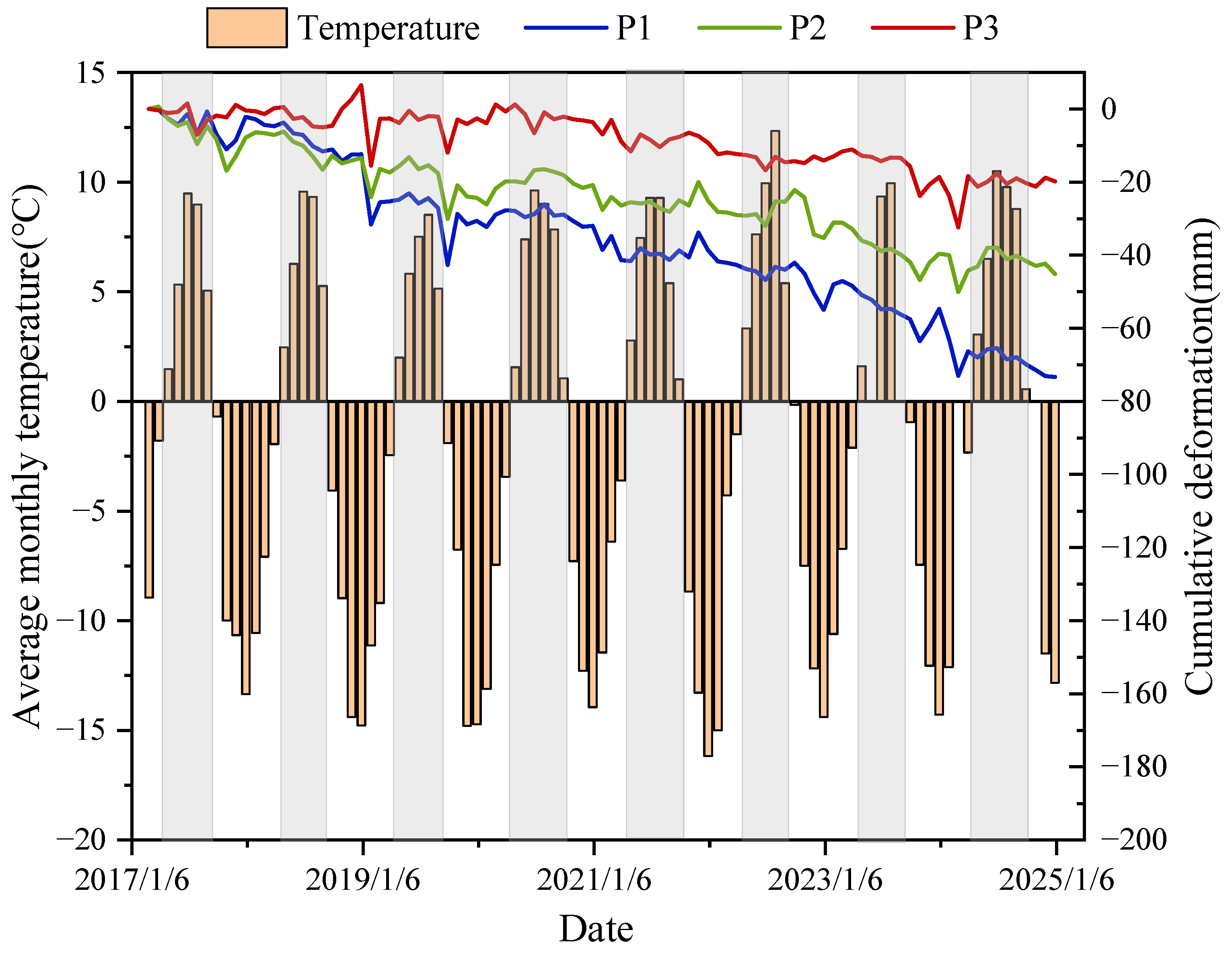
Increasing air and ground temperatures are widely recognized as crucial factors in both triggering and sustaining the activity of thaw slumps in permafrost regions [38]. Under warming climatic conditions, the thawing of ice-rich permafrost leads to a loss of soil shear strength, ground subsidence, and increased susceptibility to thaw slump development. A comparative analysis, illustrated in Figure 14 (which plots the monthly average air temperature alongside the cumulative displacement time series for P1, P2, and P3), reveals distinct spatial differences in the apparent correlation between the temperature and deformation. Point P1 (headwall/source area) exhibits the strongest apparent visual correlation with the temperature. The subsidence at P1 clearly accelerates during warm seasons, particularly when the monthly average air temperatures approach or exceed 0 °C. This strong coupling is attributed to P1’s location in the active headwall/source area, where rising temperatures directly drive the thawing of exposed ice-rich permafrost and subsequent soil instability, which illustrates a clear causal link: “rising temperature—permafrost melting—increased subsidence”. Point P2 (mid-slump) shows a moderate apparent correlation with the temperature. While the warm season temperature increases still generally coincide with periods of increased subsidence at P2, the magnitude of displacement is less than at P1, and the response appears more complex. This may reflect variations in the local ground conditions at P2, such as differences in soil composition, ice content, or drainage, leading to a more buffered or lagged response to temperature fluctuations. It underscores that deformation within the main body of the thaw slump is modulated by multiple interacting factors beyond just direct temperature forcing. Point P3 (lower/distal slump) exhibits the weakest apparent correlation with the temperature. Despite significant seasonal temperature fluctuations, the cumulative displacement at P3 remains relatively minor and shows little direct response to warm season peaks. This is consistent with P3’s location in or near the slump’s toe/accumulation zone, where the material may consist of previously thawed debris, or where the original ice-rich permafrost is now buried and less susceptible to direct atmospheric temperature influences. Consequently, temperature changes alone appear insufficient to drive significant new deformation in this more stabilized part of the feature.
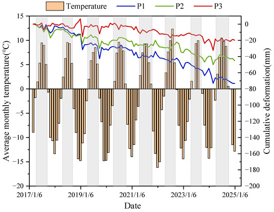
Figure 14.
Comparison of the monthly average air temperature with time series of cumulative displacement at characteristic points P1, P2, and P3.
In summary, while temperature is a core driver of thaw slump activity, its direct influence on the deformation varies significantly across different zones of the thaw slump. The deformation response to temperature fluctuations is most pronounced in the headwall/source area (represented by P1), less direct but still evident in the main transport zone (P2), and minimal in the toe/accumulation zone (P3). This spatial differentiation in temperature sensitivity reflects the varying dominant processes across the thaw slump. It underscores that assessing the influence of temperature on surface deformation requires careful consideration of the specific location within such landforms and the prevailing local ground conditions. These insights are crucial for improving the risk assessment of thaw-related geohazards in permafrost regions like the QTP.
5.2. Precipitation
Increased precipitation, particularly heavy rainfall events, can elevate soil moisture. In permafrost environments, this can accelerate the thaw of near-surface ground ice, deepen the active layer thickness, and lead to increased pore water pressures, thereby reducing the soil shear strength and contributing to thaw slump development. Figure 15, which plots precipitation alongside cumulative displacement time series for P1, P2, and P3, allows for an examination of this relationship. At point P1 (headwall/source area), a conditional correlation between the precipitation and deformation is observed. During certain periods, particularly in the warm season, episodes of significant precipitation appear to coincide with accelerated subsidence at P1. Infiltrating rainwater can accelerate ground ice thaw, increase the soil mass, and elevate the pore water pressure, and can thereby reduce the shear strength and contribute to thaw slump activity. Conversely, precipitation during cold periods (typically as snow) has a less direct or immediate impact on the deformation, though snowmelt in spring can contribute to saturated conditions. This demonstrates that the influence of precipitation on the thaw slump activity in permafrost zones is often synergistic with the temperature, with warm-season rainfall being the most effective. A weaker and less consistent correlation between the precipitation and deformation is observed at point P2 (mid-slump). Although some of the precipitation peaks correspond to increased subsidence, the overall response is smaller than that of P1, and the regularity is weaker. This attenuated response at P2 may be attributed to more complex local ground conditions, where factors such as variations in the soil texture, the ice content, and the presence of preferential drainage pathways might modulate the impact of precipitation on the ground ice thaw and soil stability. At point P3 (lower/distal slump), no significant correlation between precipitation events and the deformation is apparent. Whether the precipitation is high or low, the deformation of P3 always remains stable, and the subsidence amplitude is very small. This lack of response is consistent with P3’s location in or near the relatively stable toe/accumulation zone, where active thaw processes are less dominant and the soil structure may be less susceptible to destabilization by infiltrating precipitation.
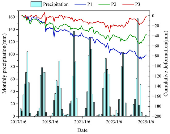
Figure 15.
Comparison of monthly total precipitation with time series of cumulative displacement (mm) at characteristic points P1, P2, and P3.
Overall, the influence of precipitation on thaw slump deformation is spatially differentiated. Precipitation appears to contribute to deformation most effectively in the headwall/source area (P1), particularly when acting synergistically with warm temperatures. Its influence is more attenuated and complex in the main transport zone (P2), and it shows little direct impact on the deformation in the toe/accumulation zone (P3). These findings highlight that precipitation often acts as a conditional cofactor in triggering thaw slump activity, with its efficacy being strongly dependent on factors such as the ambient temperature, the specific developmental stage and activity level of different zones within the slump, and the prevailing local ground conditions. This provides a key perspective for understanding the complex, multi-factorial nature of thaw-related geohazards in permafrost terrain.
5.3. Active Layer Thicknesses
The ALT refers to the depth of the ground layer that undergoes seasonal thaw in summer and refreezes in winter. Variations in the ALT directly influence the permafrost stability and the susceptibility of slopes to thaw slump development. An increase in the ALT signifies deeper seasonal thaw into the underlying permafrost, which can reduce the ground stability by warming and potentially thawing near-surface ice-rich material. Meltwater generated from this deeper thaw, if unable to drain efficiently, can accumulate at the base of the active layer (above the permafrost table). This saturation increases pore water pressures and reduces the shear strength of the soil, thereby increasing the likelihood of thaw slump initiation, particularly on slopes. Due to the scarcity of monthly ALT data, we utilized an existing annual kilometer-scale ALT dataset for overlay analysis.
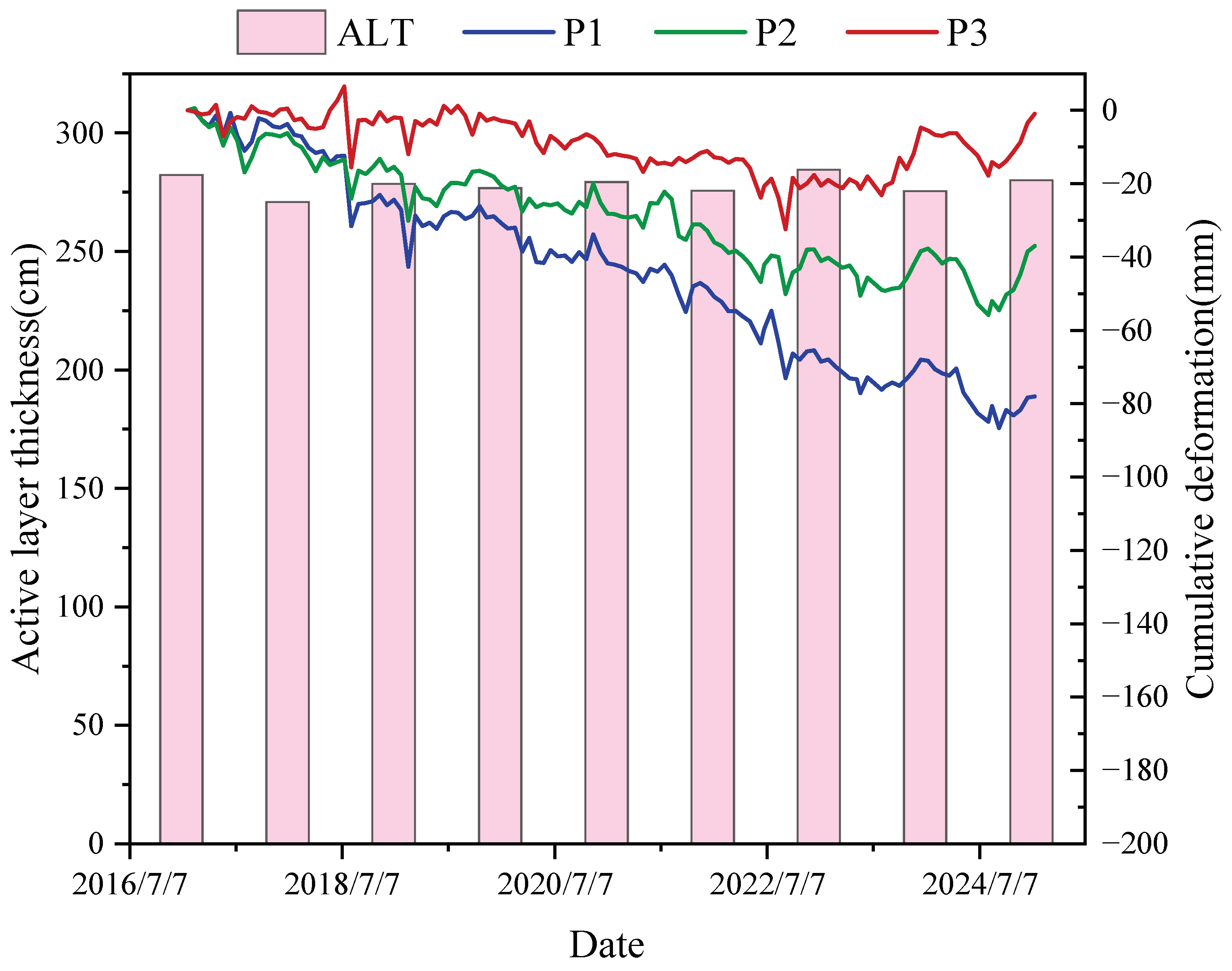
Figure 16 presents the overlay graph of the ALT with the P1, P2, and P3 time-series deformations. The ALT at the study site shows relative interannual stability, with relatively small annual fluctuations from 2017 to 2025 and without a significant deepening trend over this specific period. Despite this apparent stability in the maximum seasonal thaw depth, the cumulative displacement patterns at P1, P2, and P3 exhibit distinct behaviors. At point P1 (headwall/source area), the cumulative displacement shows a continuous and significant negative trend (subsidence). This persistent subsidence, even with a relatively stable ALT, suggests the ongoing thawing of exposed ground ice at the headwall or ice at the base of the active layer, coupled with the mechanical degradation of the soil structure due to repeated freeze–thaw cycles within the active layer. At point P2 (mid-slump), the cumulative displacement also shows an overall negative trend, though the magnitude is less than at P1, and the rate of subsidence appears to decrease in the later part of the observation period. This more moderate deformation, occurring under similar conditions of ALT stability, likely reflects differences in the local ground ice content, the soil properties, or the evolving morphology of the slump’s transport zone leading to a somewhat attenuated response to freeze–thaw processes compared to the highly active source area. At point P3 (lower/distal slump), the cumulative displacement exhibits more pronounced fluctuations without a consistent downward trend, and even shows periods of slight positive rebound in some years. This complex behavior suggests that the deformation at P3 is influenced by a combination of factors, including its location potentially within or near the depositional zone, local variations in the ground stability, the micro-topography, and, possibly, seasonal effects like frost heave or material redistribution. The differing deformation patterns observed at P1, P2, and P3, all occurring within an area characterized by a significant active layer, underscore the critical role of local heterogeneities. Factors such as the micro-topography, fine-scale variations in ground ice distribution, soil composition, and the drainage conditions likely modulate the ground’s response to seasonal thaw and freeze–thaw cycles. This leads to the observed diverse deformation characteristics across the slump feature, which emphasize that understanding thaw slump dynamics requires accounting for these site-specific variabilities in conjunction with broader environmental drivers.
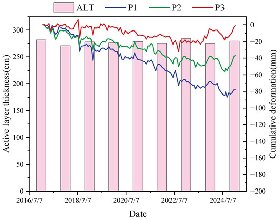
Figure 16.
Comparison of ALT with time series of cumulative displacement (mm) at characteristic points P1, P2, and P3.
5.4. Freeze-Thaw Cycle
Freeze–thaw cycles profoundly affect the shear strength of soils in permafrost zones through multiple pathways [50], and thereby influence the initiation and development of thaw slumps [51]. First, freeze–thaw processes induce significant changes in the soil structure [52]. During freezing, pore water transitions to ice, which leads to a volumetric expansion. In fine-grained soils, this process can also involve cryosuction and the formation of segregated ice lenses, which further disrupt the soil matrix. Upon thawing, this ice converts back to water, and the soil consolidates. Repeated freeze–thaw cycles can create or enlarge voids, fissures, and cracks within the soil, disrupting inter-particle bonding (cohesion) and reducing the overall integrity of the soil mass, which contributes to a reduction in the shear strength. Second, upon thawing, meltwater from ground ice (including segregated ice lenses) can lead to a significant increase in the soil moisture content and potentially supersaturated conditions if drainage is impeded. This can elevate pore water pressures, which reduces the effective inter-particle stress and consequently diminishes the frictional component of shear strength, making the soil more susceptible to shear failure. Furthermore, frozen soil typically exhibits high strength and rigidity due to the presence of ice acting as a cementing agent. Upon thawing, this ice bonding is lost, the soil structure can become loosened (especially if ice content is high), and the shear strength can decrease dramatically. This loss of strength upon thawing is a critical factor in triggering thaw slumps, particularly on slopes. As highlighted by [53], the repeated mechanical stresses during freeze–thaw cycles can also progressively degrade soil cohesion by weakening inter-particle bonds, further reducing the overall shear strength and creating conditions that are conducive to thaw slump development.
It can be observed from Figure 13 and Table 2 that the effective cohesion of soil samples shows a gradual decrease with the increase in the number of freeze–thaw cycles. This reduction in cohesion is attributed to several micro-structural changes: the volumetric expansion of water upon freezing and subsequent melting disrupts inter-particle bonds and any weak cementation. Repeated cycles alter the pore structure, which reduces the effectiveness of inter-particle contacts and the overall integrity of the soil matrix. Although the operation in this paper ensures a rigorous specification, it should be noted that the structural loss due to remodeling may deviate the absolute values of the strength parameters from those of the actual permafrost environment, which can be further verified in subsequent studies in conjunction with in situ testing or undisturbed soil sample testing.
5.5. Other Factors
The initiation and evolution of thaw slumps in the permafrost regions of the QTP result from the complex coupling of multiple environmental factors. Beyond the temperature, precipitation, ALT, and freeze–thaw effects that were discussed previously, other elements such as the vegetation cover and ground ice characteristics also play crucial roles. Vegetation cover exerts a significant influence, primarily by insulating the ground surface, which can moderate thaw depths, and by physically reinforcing the soil through root networks, which enhances its shear strength and stability. Consequently, areas with denser vegetation cover typically exhibit greater ground stability and lower susceptibility to thaw slump initiation. For instance, the depositional toe (accumulation area) of the thaw slump, where vegetation cover appears, shows less active deformation and a narrowing of the slump feature, suggesting some stabilization. Conversely, in bare or sparsely vegetated areas, such as the actively retreating headwall and the main transport zone of the thaw slump, the ground surface is more directly exposed to solar radiation and freeze–thaw processes. This lack of protection contributes to a deeper thaw, more significant soil degradation, and, consequently, more pronounced thaw slump activity and expansion. This presence of ground ice and its characteristics are fundamental preconditioning factors. Slopes underlain by ice-rich permafrost, particularly those containing massive ice bodies or high excess ice content, are inherently more susceptible. The thaw of this ground ice leads to a substantial loss of the soil shear strength, potential increases in the pore water pressure, and significant volumetric settlement (that consolidation), all of which promote gravitational failure. The local topography, particularly the slope angle and morphology, significantly influences thaw slump dynamics. The steeper slope angles observed in the headwall area (trailing edge) compared to the gentler slopes at the toe (leading edge) contribute to higher gravitational shear stresses at the headwall, promoting active retreat and failure. This local slope difference contributes to the observed pattern of rapid headwall retreat and more gradual movement and deposition in the gentler toe area, which result in spatially variable rates of activity across the slump. Loose or unconsolidated soils with an inherently low thawed shear strength, such as chalky soils or poorly graded gravels, are particularly susceptible. Similarly, bedrock with extensive fracturing can be prone to instability when subjected to freeze–thaw processes, though the analyzed site appears to be dominated by surficial deposits. In addition, compared with sunny slopes, shady slopes receive less direct solar radiation, which can lead to colder ground temperatures, potentially thicker and more persistent snow cover, reduced evapotranspiration, higher soil moisture content, and, consequently, more favorable conditions for the preservation and development of thick ground ice. These conditions can render shady slopes more susceptible to thaw slumps [32].
6. Conclusions
This study investigated the deformation characteristics, kinematic patterns, and driving mechanisms of the thaw slump on the Qinghai-Tibetan Plateau. We utilized Sentinel-1A SAR data from March 2017 to January 2025 with the Small Baseline Subset (SBAS) InSAR technique to derive the time-series deformation, and through the integration of ascending and descending orbit data with a surface-parallel flow constraint, its three-dimensional (3D) displacement field. The influence of climatic factors (temperature and precipitation) and the active layer thickness (ALT) on thaw slump activity was analyzed by correlating deformation patterns with meteorological records and contextual ALT data. In addition, laboratory direct shear tests were conducted on site-specific soil samples subjected to different numbers of freeze–thaw cycles to quantify changes in shear strength and understand the role of freeze–thaw-induced soil weakening in thaw slump development. The main conclusions drawn from this multi-faceted investigation are as follows:
- The mean annual deformation rates of the thaw slump ranged from −17.55 mm/year (subsidence) to +5.72 mm/year (uplift). The net settlement was primarily observed within the demarcated boundary of the melting and slump zone, while the deformation in most areas outside this boundary was relatively minor. The intensity of subsidence generally decreased from the headwall/source area (near P1) towards the more distal parts (P2, P3). The deformation rate profile revealed the characteristic of “subsidence at both ends and localized uplift in the middle”, and the deformation rate at different locations varied significantly, indicating that the internal deformation of the thaw slump has significant spatial non-uniformity;
- The total cumulative displacement from 2017 to 2025 ranged from −199.5 mm (subsidence) to +55.9 mm (uplift). Time-series analyses revealed inter-annual variations in the deformation intensity, with the most significant subsidence being concentrated in the upper/southern (headwall/source) part of the thaw slump. Overall, the thaw slump exhibited persistent activity and complex spatiotemporal dynamics throughout the observation period. Characteristic points P1 and P2 experienced substantial and continuous subsidence, while P3 showed a more subdued and lagged deformation response, reflecting its location and local ground conditions;
- The thaw slump exhibits an elongated morphology. The 3D deformation analysis revealed that the horizontal displacement rates/magnitudes are significantly higher within the delineated thaw slump boundary compared to the surrounding terrain. This horizontal movement predominantly occurs from south to north, which is consistent with field observations of the slump’s overall orientation and downslope progression. The minimal deformation observed outside the boundary highlights the localized nature of the significant ground instability associated with this active thaw slump feature;
- The initiation and ongoing development of the thaw slump result from the coupled influence of multiple factors. Temperature is a core driver, with its influence on the deformation varying significantly across different zones of the slump. Precipitation acts as a conditional cofactor, with its impact also being spatially dependent and often synergistic with warm temperatures. The presence of a significant active layer overlying highly ice-rich permafrost establishes the fundamental susceptibility of the site to thaw-induced instability. Finally, laboratory tests demonstrated that repeated freeze–thaw cycles progressively degrade soil shear strength (reducing both cohesion and friction angle), a mechanism that contributes to the weakening of active layer materials and facilitates the development and reactivation of thaw slumps.
Although the deformation characteristics of the studied thaw slump were revealed by the fusion of multi-source data in this study, there are still limitations to our method. Meteorological data were collected from the Tuotuohe station, which is about 82 km away from the study area, and the difference in the microclimate of the QTP may cause the temperature and humidity conditions to deviate from the actual situation. The boundaries of the thaw slump are based on UAV images taken in August 2024, and the static boundaries fail to reflect the dynamic evolution process of the thaw slump, which limits the accuracy of our deformation analysis. The three-dimensional deformation inversion relies on the SPF assumption and uses only the ascending and descending orbit dual line-of-sight data, which is not a strict three-dimensional solution. In the future, it is necessary to combine local meteorological, dynamic boundary, and multi-track data to realize the full three-dimensional solution of this method.
Author Contributions
Conceptualization, Z.Y. and W.N.; Data curation, Z.Y. and S.R.; Methodology, Z.Y. and S.R.; Project administration, W.N. and S.Z.; Supervision, W.N. and H.W.; Writing—original draft, Z.Y. and W.N.; Writing—review and editing, Z.Y. and P.A. All authors have read and agreed to the published version of the manuscript.
Funding
This research was supported by the Grants of National Natural Science Foundation of China (No. 42171125); the Second Tibetan Plateau Scientific Expedition and Research (STEP) program (Grant No. 2019QZKK0905); the Natural Science Foundation of Shaanxi Province (Grant no. 2024JC-YBMS-314).
Data Availability Statement
Data openly available in a public repository.
Conflicts of Interest
The authors declare no conflicts of interest.
References
- Cheng, G.; Zhao, L.; Li, R.; Wu, X.; Sheng, Y.; Hu, G.; Zou, D.; Jin, H.; Li, X.; Wu, Q. Characteristic, changes and impacts of permafrost on Qinghai-Tibet Plateau. Chin. Sci. Bull. 2019, 64, 2783–2795. [Google Scholar]
- Zou, D.; Zhao, L.; Sheng, Y.; Chen, J.; Hu, G.; Wu, T.; Wu, J.; Xie, C.; Wu, X.; Pang, Q.; et al. A new map of permafrost distribution on the Tibetan Plateau. Cryosphere 2017, 11, 2527–2542. [Google Scholar] [CrossRef]
- Yang, Z.; Ni, W.; Niu, F.; Li, L.; Ren, S. Spatiotemporal Distribution Characteristics and Influencing Factors of Freeze-Thaw Erosion in the Qinghai-Tibet Plateau. Remote Sens. 2024, 16, 1629. [Google Scholar] [CrossRef]
- Li, L.; Feng, H.; Chen, K. Causes analysis and countermeasures for engineering distress in embankment-bridge transition section of the Qinghai-Xizang Railway in permafrost regions. J. Glaciol. Geocryol. 2025, 47, 199–212. [Google Scholar]
- Niu, F.; Wang, W.; Lin, Z.; Luo, J. Study on Environmental and Hydrological Effects of Thermokarst Lakes in Permafrost Regions of the Qinghai-Tibet Plateau. Adv. Earth Sci. 2018, 33, 335–342. [Google Scholar]
- Peng, X.; Frauenfeld, O.W.; Cao, B.; Wang, K.; Wang, H.; Su, H.; Huang, Z.; Yue, D.; Zhang, T. Response of changes in seasonal soil freeze/thaw state to climate change from 1950 to 2010 across China. J. Geophys. Res. Earth Surf. 2016, 121, 1984–2000. [Google Scholar] [CrossRef]
- Wang, K.; Zhang, T.; Zhong, X. Changes in the timing and duration of the near-surface soil freeze/thaw status from 1956 to 2006 across China. Cryosphere 2015, 9, 1321–1331. [Google Scholar] [CrossRef]
- Guo, D.; Wang, H. CMIP5 permafrost degradation projection: A comparison among different regions. J. Geophys. Res. Atmos. 2016, 121, 4499–4517. [Google Scholar] [CrossRef]
- Guodong Cheng, L.Z.; Cheng, G.; Zhao, L. The problem of frozen soil in the development of the Qinghai Tibet Plateau. Quat. Sci. 2000, 20, 521–531. [Google Scholar] [CrossRef]
- Huscroft, C.A.; Lipovsky, P.; Bond, J.D. Permafrost and landslide activity: Case studies from southwestern Yukon Territory. In Yukon Exploration and Geology 2003; Emond, D.S., Lewis, L.L., Eds.; Yukon Geological Survey: Whitehorse, YT, Canada, 2003; pp. 107–119. [Google Scholar]
- Niu, F.Z.L.; Yu, Q.; Xie, Q. Study on Slope Types and Stability of Typical Slopes in Permafrost Regions of the Tibetan Plateau. J. Glaciol. Geocryol. 2002, 24, 608–613. [Google Scholar]
- Woods, G.C.; Simpson, M.J.; Pautler, B.G.; Lamoureux, S.F.; Lafreniere, M.J.; Simpson, A. Evidence for the enhanced lability of dissolved organic matter following permafrost slope disturbance in the Canadian High Arctic. Geochim. Cosmochim. Acta 2011, 75, 7226–7241. [Google Scholar] [CrossRef]
- Schuur, E.A.G.; McGuire, A.D.; Schaedel, C.; Grosse, G.; Harden, J.W.; Hayes, D.J.; Hugelius, G.; Koven, C.D.; Kuhry, P.; Lawrence, D.M.; et al. Climate change and the permafrost carbon feedback. Nature 2015, 520, 171–179. [Google Scholar] [CrossRef] [PubMed]
- Turetsky, M.R.; Abbott, B.W.; Jones, M.C.; Anthony, K.W.; Olefeldt, D.; Schuur, E.A.G.; Koven, C.; McGuire, A.D.; Grosse, G.; Kuhry, P.; et al. Permafrost collapse is accelerating carbon release. Nature 2019, 569, 32–34. [Google Scholar] [CrossRef] [PubMed]
- Luo, J.; Niu, F.; Lin, Z.; Liu, M.; Yin, G.; Gao, Z. The characteristics and patterns of retrogressive thaw slumps developed in permafrost region of the Qinghai-Tibet Plateau. J. Glaciol. Geocryol. 2022, 44, 96–105. [Google Scholar]
- French, H.M. The Periglacial Environment [M]; John Wiley & Sons: Hoboken, NJ, USA, 2017. [Google Scholar]
- Luo, J.; Niu, F.; Lin, Z.; Liu, M.; Yin, G.; Gao, Z. Inventory and Frequency of Retrogressive Thaw Slumps in Permafrost Region of the Qinghai-Tibet Plateau. Geophys. Res. Lett. 2022, 49, e2022GL099829. [Google Scholar] [CrossRef]
- Niu, F.; Luo, J.; Lin, Z.; Fang, J.; Liu, M. Thaw-induced slope failures and stability analyses in permafrost regions of the Qinghai-Tibet Plateau, China. Landslides 2016, 13, 55–65. [Google Scholar] [CrossRef]
- Jiang, G.; Gao, S.; Lewkowicz, A.G.; Zhao, H.; Pang, S.; Wu, Q. Development of a rapid active layer detachment slide in the Fenghuoshan Mountains, Qinghai-Tibet Plateau. Permafr. Periglac. Process. 2022, 33, 298–309. [Google Scholar] [CrossRef]
- Li, Y.; Liu, Y.; Chen, J.; Dang, H.; Zhang, S.; Mei, Q.; Zhao, J.; Wang, J.; Dong, T.; Zhao, Y. Advances in retrogressive thaw slump research in permafrost regions. Permafr. Periglac. Process. 2024, 35, 125–142. [Google Scholar] [CrossRef]
- Shao, T.; Zheng, Z.; He, Y.; Huang, W.; Xie, C. Monitoring Geological Hazards with InSAR. In Proceedings of the 2022 IEEE International Geoscience and Remote Sensing Symposium (IGARSS 2022), Kuala Lumpur, Malaysia, 17–22 July 2022; pp. 2558–2561. [Google Scholar]
- Lu, Z.; Yang, H.; Zeng, W.; Liu, P.; Wang, Y. Geological Hazard Identification and Susceptibility Assessment Based on MT-InSAR. Remote Sens. 2023, 15, 5316. [Google Scholar] [CrossRef]
- Zhong, J.; Li, Q.; Zhang, J.; Luo, P.; Zhu, W. Risk Assessment of Geological Landslide Hazards Using D-InSAR and Remote Sensing. Remote Sens. 2024, 16, 345. [Google Scholar] [CrossRef]
- Yue, J.; Yue, S.; Qiu, Z.; Wang, X.; Guo, L. Research on the method of extracting DEM based on GBInSAR. Laser Radar Technol. Appl. XXI 2016, 9832, 98320J. [Google Scholar]
- Hu, J. Research on Land Subsidence Monitoring in Beijing Based on Multiple InSAR Technologies. Master’s Thesis, Chang’an University, Xi’an, China, 2023. [Google Scholar]
- Hooper, A. A multi-temporal InSAR method incorporating both persistent scatterer and small baseline approaches. Geophys. Res. Lett. 2008, 35, L16302. [Google Scholar] [CrossRef]
- Iglesias, R.; Mallorqui, J.J.; Monells, D.; Lopez-Martinez, C.; Fabregas, X.; Aguasca, A.; Gili, J.A.; Corominas, J. PSI Deformation Map Retrieval by Means of Temporal Sublook Coherence on Reduced Sets of SAR Images. Remote Sens. 2015, 7, 530–563. [Google Scholar] [CrossRef]
- Chen, J.; Wu, T.; Zou, D.; Liu, L.; Wu, X.; Gong, W.; Zhu, X.; Li, R.; Hao, J.; Hu, G.; et al. Magnitudes and patterns of large-scale permafrost ground deformation revealed by Sentinel-1 InSAR on the central Qinghai-Tibet Plateau. Remote Sens. Environ. 2022, 268, 112778. [Google Scholar] [CrossRef]
- Si, J.; Zhang, S.; Niu, Y.; Zhang, Y.; Fan, Q.; Chen, Y. The surface deformation of permafrost and active layer thickness in the upper reaches of the Black River basin, revealed by InSAR observations and independent component analysis. Sci. Total Environ. 2024, 951, 175667. [Google Scholar] [CrossRef]
- Berardino, P.; Fornaro, G.; Lanari, R.; Sansosti, E. A new algorithm for surface deformation monitoring based on small baseline differential SAR interferograms. IEEE Trans. Geosci. Remote Sens. 2002, 40, 2375–2383. [Google Scholar] [CrossRef]
- Yang, S.; Li, D.; Liu, Y.; Xu, Z.; Sun, Y.; She, X. Landslide Identification in Human-Modified Alpine and Canyon Area of the Niulan River Basin Based on SBAS-InSAR and Optical Images. Remote Sens. 2023, 15, 1998. [Google Scholar] [CrossRef]
- Liu, Y.; Qiu, H.; Wang, J.; Wang, N.; Jiang, X.; Tang, B.; Yang, D.; Ye, B.; Kamp, U. Prominent creep characteristics of thermokarst landslides on central Tibetan Plateau under climate warming conditions. Catena 2024, 246, 108457. [Google Scholar] [CrossRef]
- Zhao, R.; Li, Z.-w.; Feng, G.-c.; Wang, Q.-j.; Hu, J. Monitoring surface deformation over permafrost with an improved SBAS-InSAR algorithm: With emphasis on climatic factors modeling. Remote Sens. Environ. 2016, 184, 276–287. [Google Scholar] [CrossRef]
- Jiao, Z.; Xu, Z.; Guo, R.; Zhou, Z.; Jiang, L. Potential of Multi-temporal InSAR for Detecting Retrogressive Thaw Slumps: A Case of the Beiluhe Region of the Tibetan Plateau. Int. J. Disaster Risk Sci. 2023, 14, 523–538. [Google Scholar] [CrossRef]
- Xue, Z.; Zhao, S.; Zhang, B. Study on Soil Freeze-Thaw and Surface Deformation Patterns in the Qilian Mountains Alpine Permafrost Region Using SBAS-InSAR Technique. Remote Sens. 2024, 16, 4595. [Google Scholar] [CrossRef]
- Deng, H.; Zhang, Z.; Wu, Y. Accelerated permafrost degradation in thermokarst landforms in Qilian Mountains from 2007 to 2020 observed by SBAS-InSAR. Ecol. Indic. 2024, 159, 111724. [Google Scholar] [CrossRef]
- Li, L. Study on the Evolution and Eco-Environmental Effects of Lakes in the Qinghai-Tibet Plateau. Ph.D. Thesis, Chang’an University, Xi’an, China, 2021. [Google Scholar]
- Wang, F.; Wen, Z.; Gao, Q.; Yu, Q.; Li, D.; Chen, L. Creep features and mechanism of active-layer detachment slide on the Qinghai-Tibet Plateau by InSAR. Catena 2024, 237, 107782. [Google Scholar] [CrossRef]
- Jiao, C. Quantitative Assessment of Retrogressive Thaw Slump Induced Soil Erosion in Permafrost Regions on the Qinghai-Tibet Plateau. Ph.D. Thesis, South China University of Technology, Guangzhou, China, 2023. [Google Scholar]
- Cao, Z.T.; Nan, Z.T.; Hu, J.N.; Chen, Y.H.; Zhang, Y.N. A new 2010 permafrost distribution map over the Qinghai-Tibet Plateau based on subregion survey maps: A benchmark for regional permafrost modeling. Earth Syst. Sci. Data 2023, 15, 3905–3930. [Google Scholar] [CrossRef]
- Luo, J.; Niu, F.; Lin, Z.; Liu, M.; Yin, G. Recent acceleration of thaw slumping in permafrost terrain of Qinghai-Tibet Plateau: An example from the Beiluhe Region. Geomorphology 2019, 341, 79–85. [Google Scholar] [CrossRef]
- Lu, P.; Han, J.; Yi, Y.; Hao, T.; Zhou, F.; Meng, X.; Zhang, Y.; Li, R. MT-InSAR Unveils Dynamic Permafrost Disturbances in Hoh Xil (Kekexili) on the Tibetan Plateau Hinterland. IEEE Trans. Geosci. Remote Sens. 2023, 61, 1–16. [Google Scholar] [CrossRef]
- Wei, Y.; Qiu, H.; Liu, Z.; Huangfu, W.; Zhu, Y.; Liu, Y.; Yang, D.; Kamp, U. Refined and dynamic susceptibility assessment of landslides using InSAR and machine learning models. Geosci. Front. 2024, 15, 101890. [Google Scholar] [CrossRef]
- Gong, W.; Darrow, M.M.; Meyer, F.J.; Daanen, R.P. Reconstructing movement history of frozen debris lobes in northern Alaska using satellite radar interferometry. Remote Sens. Environ. 2019, 221, 722–740. [Google Scholar] [CrossRef]
- Cai, J.; Wang, X.; Wu, T.; Wu, R.; Liu, G. Characterizing the kinematics of active rock glaciers in Daxue Shan, southeastern Tibetan plateau, using SAR interferometry and generalized boosted modeling. Remote Sens. Environ. 2024, 313, 114352. [Google Scholar] [CrossRef]
- Joughin, I.; Kwok, R.; Fahnestock, M. Estimation of ice-sheet motion using satellite radar interferometry: Method and error analysis with application to Humboldt Glacier, Greenland. J. Glaciol. 1996, 42, 564–575. [Google Scholar] [CrossRef]
- Shi, H. Freezing and Thawing on the Physical and Mechanical Properties of Loess and Engineering Applications. Master’s Thesis, Chang’an University, Xi’an, China, 2013. [Google Scholar]
- Xiao, D.; Feng, W.; Zhang, Z. The changing rule of loess’s porosity under freezing-thawing cycles. J. Glaciol. Geocryol. 2014, 36, 907–912. [Google Scholar]
- Hawke, R.; McConchie, J. In situ measurement of soil moisture and pore-water pressures in an ‘incipient’ landslide: Lake Tutira, New Zealand. J. Environ. Manag. 2011, 92, 266–274. [Google Scholar] [CrossRef] [PubMed]
- Wang, B.; Liu, J.; Wang, Q.; Ling, X.; Pan, J.; Fang, R.; Bai, Z. Influence of freeze-thaw cycles on the shear performance of silty clay-concrete interface. Cold Reg. Sci. Technol. 2024, 219, 104120. [Google Scholar] [CrossRef]
- Yu, Y.; Zhang, Z.; Dai, F.; Bai, S. A New Shear Strength Model with Structural Damage for Red Clay in the Qinghai-Tibetan Plateau. Appl. Sci. 2024, 14, 3169. [Google Scholar] [CrossRef]
- Kong, F. Study on the Evolution and Mechanism of Water Erosion Characteristics of Soda-Saline Soil Under Freeze-Thaw and Wet-Dry Cycles. Ph.D. Thesis, Jilin University, Changchun, China, 2024. [Google Scholar]
- Xie, S.; Qu, J.; Lai, Y.; Zhou, Z.; Xu, X. Effects of freeze-thaw cycles on soil mechanical and physical properties in the Qinghai-Tibet Plateau. J. Mt. Sci. 2015, 12, 999–1009. [Google Scholar] [CrossRef]


Disclaimer/Publisher’s Note: The statements, opinions and data contained in all publications are solely those of the individual author(s) and contributor(s) and not of MDPI and/or the editor(s). MDPI and/or the editor(s) disclaim responsibility for any injury to people or property resulting from any ideas, methods, instructions or products referred to in the content. |
© 2025 by the authors. Licensee MDPI, Basel, Switzerland. This article is an open access article distributed under the terms and conditions of the Creative Commons Attribution (CC BY) license (https://creativecommons.org/licenses/by/4.0/).