Article

Preliminary Study on Near-Surface Air Temperature Lapse Rate Estimation and Its Spatiotemporal Distribution Characteristics in Beijing–Tianjin–Hebei Mountainous Region

1
School of Remote Sensing and Geomatics Engineering, Nanjing University of Information Science & Technology, Nanjing 210044, China
2
School of Civil Engineering, Nanjing Forestry University, Nanjing 210037, China
3
School of Geographical Sciences, Nanjing University of Information Science & Technology, Nanjing 210044, China
4
Changwang School of Honors, Nanjing University of Information Science & Technology, Nanjing 210044, China
*
Author to whom correspondence should be addressed.
Remote Sens. 2025, 17(13), 2205; https://doi.org/10.3390/rs17132205
Submission received: 7 May 2025 / Revised: 10 June 2025 / Accepted: 25 June 2025 / Published: 26 June 2025

Abstract

The near-surface air temperature lapse rate (SATLR) is a crucial parameter in climate, hydrology, and ecology research conducted in mountainous regions. However, existing research has difficulty characterizing its dynamic changes on an hourly scale. Obtaining data with high spatiotemporal resolution in complex terrains using existing methods poses challenges. This study introduces a hierarchical method for estimating SATLR at high spatiotemporal resolutions based on Fengyun-4A (FY-4A) Advanced Geostationary Radiation Imager (AGRI) land surface temperature (LST) data and machine learning techniques. Based on reconstructed FY-4A AGRI LST data, this study downscales the 4 km resolution data to a 1 km resolution using machine learning. It then estimates the spatial distribution of near-surface air temperature (SAT) and normalized near-surface air temperature (nSAT) by integrating station observations. Subsequently, high spatiotemporal resolution SATLRs are estimated, and their spatial and temporal distribution characteristics in the Beijing–Tianjin–Hebei mountainous region are analyzed. The results indicate that the SATLR exhibits a predominant distribution of 2~6 °C/km annually across the study area. However, in specific regions such as Taihang Mountains in the southwest, Damajun Mountain in the northwest, and certain areas of central Beijing City, the SATLR exceeds 6 °C/km in depth. Conversely, in Chengde City in the northeast and Huapiling in Damajun Mountain in the northwest, the SATLR is shallower than 2 °C/km. Seasonally, the average SATLR displays significant variation, with 3~5 °C/km being prevalent in spring, summer, and autumn, and 2~4 °C/km in winter. Moreover, the diurnal SATLR patterns from the second to fifth altitude grades exhibit consistency throughout the year and across seasons, albeit with varying overall values at different altitudes. Notably, the SATLR of the first altitude grade demonstrates stability within a day at lower elevations.

1. Introduction

Temperature lapse rate (TLR) refers to the decrease in temperature with the increase in altitude, also known as vertical temperature gradient [1], which usually includes the land temperature lapse rate (LTLR), near-surface air temperature lapse rate (SATLR), free atmosphere temperature lapse rate (FATLR), and others [2]. In meteorology, the SATLR is particularly important for complex mountainous areas with insufficient temperature observation data, and is widely used in the research fields of temperature spatial distribution interpolation, modeling forecast temperature correction, temperature downscaling and so on. The SATLR is one of the important input parameters for hydrological, glaciological and ecological models. It is used to simulate hydrological models in mountain areas, melt glaciers and permafrost, and study climate warming rates related to altitude. Therefore, obtaining the spatiotemporal distribution of SATLR with high accuracy holds significant importance for scientific research and regional sustainable development [1,3].
On a worldwide scale, the temperature is generally observed to decrease by 6.5 °C for each kilometer increase in elevation. Nevertheless, the SATLR varies significantly over time and space in certain regions due to factors such as seasonality, terrain characteristics, surface composition, humidity levels, weather patterns, solar radiation, wind velocity and other microclimatic variables.
Currently, researchers worldwide have conducted SATLR studies in mountainous regions primarily utilizing data from meteorological stations. Kirchner et al. examined the SATLR in the Alps Valley by analyzing long-term data from the Garmisch-Partenkirchen Valley and Zugfeng meteorological stations in Germany spanning from 1936 to 2008 [4]. Their analysis highlighted the significant impact of season and weather patterns on the SATLR. They observed that the rapid warming of the valley bottom in recent decades has resulted in a steep SATLR, averaging −6.2 °C/km annually. Li Xiuping et al. investigated the SATLR in the Daxing’anling Prefecture using temperature data from 553 meteorological stations nationwide [5]. They identified a notably higher SATLR in this region compared to the national average, ranging from 7 °C/km to 9 °C /km. They noted that the spatial variation is most pronounced in winter and exhibits a significant positive correlation with temperature, while showing a negative correlation with humidity. Shen et al. conducted a comparative analysis of SATLR changes on the north and south slopes of the Tianshan Mountains and within the inner Tianshan Mountains [6]. Their analysis was based on temperature observations from meteorological stations on both slopes and the Kaidu River Basin in the Tianshan Mountains. Córdova et al. conducted a novel study to assess the rate of temperature decrease near the surface in the southern Ecuadorian Andes. Over an 18-month period, they collected data from nine stations spanning an elevation range of 2600–4200 m. Their analysis revealed annual mean temperature values (Tmean: 6.88 °C/km) in line with conventional norms, while Tmax (8.80 °C/km) and Tmin (5.48 °C/km) showed significant deviations from the MTCLIM model’s default values (6 °C/km and 3 °C/km). The study demonstrated that accurate calculation of the lapse rate can be achieved with only 2–3 stations, highlighting the influential role of high-altitude cloud cover and humidity in reducing the diurnal temperature range [7].
However, the rugged terrain and limited transportation infrastructure in mountainous regions result in sparse distribution of meteorological stations, leading to insufficient acquisition of meteorological data [3]. This makes it challenging to obtain SATLR with continuous spatiotemporal distributions. Thermal infrared satellite imagery offers an effective solution by enabling rapid and synchronous acquisition of large-scale, continuous two-dimensional spatial distribution data for land surface temperature (LST) [8,9,10,11,12]. These datasets can be utilized to estimate LTLR or calculate SATLR through temperature estimation models, thereby providing novel approaches for studying SATLR spatiotemporal patterns [13]. For instance, Wang Yanxia et al. integrated MODIS-derived LST products with 30-year meteorological station data and a digital elevation model (DEM) to analyze SATLR in Yunnan’s mountainous regions. Their study revealed that after accounting for micro-terrain effects, the average lapse rate across the region is 5.3 °C/km, which differs from traditional observations. Specifically, the SATLR is shallowest in the high mountain areas of northwest Yunnan and steepest in the low mountain regions of southern Yunnan [14]. Moreover, the SATLR shows a gradual increase from sunny slopes to shady slopes, underscoring the notable impact of micro-terrain on the air temperature distribution. Romshoo et al. conducted a study in the Kashmir Himalayas to model the LTLR by analyzing the relationship between MODIS LST and GTOPO30 DEM [15]. Their findings revealed spatiotemporal variations in LTLR ranging from 3 °C to 12 °C per kilometer. Firozjaei et al. proposed an enhanced approach for modeling LTLR by standardizing normalized LST (NLST) and DEM data to create a feature space using remote sensing data from Landsat, MODIS and ASTER DEM, in conjunction with ground-based air temperature measurements from meteorological stations. The study demonstrated that the NLST-DEM, as compared to the conventional LST-DEM, yielded an increase in R2 ranging from 0.30 to 0.42 and a decrease in root mean square error (RMSE) by 8.1 °C to 9.4 °C per kilometer across three study areas [3]. These results validate the efficacy of normalization techniques in improving the accuracy of SATLR modeling in complex terrain environments.
Considerable progress has been achieved in the comprehensive analysis of mountain SATLR estimation and temporal and spatial distribution both domestically and internationally. However, certain deficiencies persist, including the limited number and geographical coverage of meteorological observation stations, as well as the inadequate representativeness of various topographic factors. Consequently, the data from these stations fail to accurately capture the spatial variability of the SATLR in small, synchronous and continuous mountainous terrains. Remote sensing retrieval of LST (or air temperature) offers a continuous estimation of SATLR spatial distribution. This method enables the comparative analysis of SATLRs across diverse geographical locations. Due to the specific orbit of satellites and the impact of weather conditions during imaging, remote sensing methods can only capture LSTs under clear skies during satellite passes. Consequently, only a limited number of remote sensing-derived surface or air temperatures are available for calculating and analyzing SATLR. This limitation precludes obtaining high temporal resolution SATLR continuously. Existing studies primarily examine variations in mean, shallowest, and deepest SATLR on monthly, seasonal, annual and multi-year time scales. The characteristics of SATLR at different geographical locations and hourly resolutions remain unclear, posing significant challenges for various applications requiring high-temporal-resolution temperature data over complex terrains.
This study utilizes high-temporal-resolution data provided by the Advanced Geostationary Radiation Imager (AGRI) aboard the Fengyun-4A satellite (FY-4A). Based on LST reconstruction, machine learning methods are employed to reduce the spatial resolution of LST data from 4 km to 1 km. By integrating station observation temperature data, the spatial distribution of near-surface air temperature (SAT) is estimated, enabling the calculation of high-resolution SATLRs. The investigation specifically delves into the spatiotemporal characteristics of SATLRs in the mountainous region of Beijing–Tianjin–Hebei (BTH). The primary objective is to develop a method for accurately determining SATLRs at high spatiotemporal resolutions. The findings aim to offer insights into the spatiotemporal patterns of SATLR in the BTH area, thereby facilitating the assessment and characterization of SATLRs in geographically intricate terrains.

2. Materials and Methods

2.1. Study Area

This study focuses on the BTH region, as shown in Figure 1, spanning approximately 216,000 square kilometers between 36°03′ to 42°40′N and 113°27′ to 119°50′E. The area encompasses diverse geomorphological features such as mountains, plateaus, and valleys, resulting in significant surface heterogeneity. The altitude gradient in the region ranges from −5 m in Bohai Bay to 2882 m in Xiaowutai Mountain. The interaction between monsoon circulation and topographic elevation leads to a pronounced vertical climate variation. This is evident in the southeastern areas where warm and moist air currents generate a precipitation front (annual precipitation > 700 mm) at the eastern base of Taihang Mountain. Conversely, locations like Chengde, situated at the northern foothills of Yanshan Mountain, experience the impact of winter monsoon subsidence, resulting in over 40 days of inversion per year. The area exhibits high levels of human activity, ranking among the most intense globally. The urban heat island effect within the Beijing–Tianjin–Baoding metropolitan area contributes to a more rapid warming trend at lower elevations (0.35 °C/10a) compared to mountainous regions (0.18 °C/10a). Consequently, a combination of “natural gradient” and “anthropogenic disturbance” influences the SATLR in this region. Elevations range from −5 m in Bohai Bay to 2882 m at Xiaowutai Mountain, the primary peak of the Taihang mountain range. The region exhibits an average elevation of 412 m and a surface slope of 9.7°, with the core of the Yanshan Mountains area having an average slope of 21.3° and the Bashang Plateau averaging 7.5°, indicative of stepped terrain characteristics. The prevailing climate is warm temperate semi-humid, with mean annual air temperatures and precipitation levels of 10.8 °C and 526 mm, respectively. However, due to vertical variations in terrain, annual precipitation ranges from 720 mm in the southern Yanshan Mountains foothills to 380 mm in the Sanggan River valley. The primary underlying surface in the study area is the Yanshan–Taihang Mountains ecological barrier zone, comprising mountain forest belts (warm temperate deciduous broadleaved forest, coniferous broadleaved mixed forest, subalpine meadow), valley shrub belts, and pastoral transition zones. Vegetation coverage demonstrates distinct vertical stratification, increasing from 0.32 in valley areas to 0.78 in mountain ecological zones.

2.2. Data

2.2.1. FY-4A AGRI L2 LST

This study employs the Level-2 LST product from the Advanced Geostationary Radiation Imager (AGRI) onboard the Fengyun-4A (FY-4A) satellite, derived through the split-window algorithm using thermal infrared bands 12 (10.3–11.3 μm) and 13 (11.5–12.5 μm). The FY-4A AGRI performs full-disk scans every 15 min, delivering continuous temperature observations at hourly temporal resolution and 4 km spatial resolution. Data are stored in NetCDF files under a nominal projection coordinate system.
All data from the year 2020 were selected as the study periods. Hourly AGRI LST datasets were obtained from the Fengyun Satellite Remote Sensing Data Service (https://satellite.nsmc.org.cn/, accessed on 10 April 2023)). Each data file includes a quality control (QC) marker layer, employing a five-level classification system: Grade 1 signifies an inversion error of less than 2 K, Grade 2 ranges from 2 to 3 K, and Grades 3 and higher represent invalid data. Only high-quality data with QC scores ≤ 1 were included in the analysis. The nominal projection of the FY4A LST data underwent conversion to the WGS 1984 coordinate system utilizing positioning data.

2.2.2. NASA DEM Data

The study utilizes the NASA digital elevation model (DEM) with 30 m resolution, publicly released by the National Aeronautics and Space Administration (NASA). This DEM dataset covers global land surfaces between 60°N and 56°S latitudes, accessible through the EarthData portal (https://search.earthdata.nasa.gov, accessed on 15 April 2025). Generated through enhanced algorithms incorporating Shuttle Radar Topography Mission (SRTM) raw radar signals with multi-source data fusion (including ASTER GDEM and ICESat GLAS satellite observations), the dataset achieves improved vertical accuracy and effective void filling. Slope gradients were calculated from the DEM, with both elevation and slope serving as terrain explanatory variables within the LST downscaling framework, SAT estimation model, and SATLR calculation procedures.

2.2.3. ERA5-Land Reanalysis Data

The ERA5-Land surface reanalysis dataset, developed by the European Centre for Medium-Range Weather Forecasts (ECMWF), enhances land surface process characterization through integration of ERA5 atmospheric forcing variables and simulation with the upgraded Hydrology Tiled ECMWF Scheme for Surface Exchanges over Land (HTESSEL) model (version CY45R1). Demonstrating superior spatiotemporal resolution (0.1°) and accuracy compared to previous versions, this dataset provides global hourly land surface parameters from 1950 onward via the Copernicus Climate Data Store (https://cds.climate.copernicus.eu/, accessed on 10 April 2023). For this study, ERA5-Land data products encompassing cumulative net shortwave radiation (SNSR), cumulative net terrestrial radiation (SNTR), and cumulative downward shortwave radiation (SSR) were acquired. The net radiation flux (SNR), derived from the summation of SNSR and SNTR, serves as the radiative forcing component for LST modeling. SSR is used for the downscaling of the LST, the estimation of SAT, and the estimation of the SATLR.

2.2.4. MODIS Products

Three MODIS data products were utilized in this study: MCD43A3, providing 16-day synthetic surface albedo data at a 500 m spatial resolution; MOD13 A2, offering 16-day synthetic surface albedo data at a 1 km spatial resolution; and MOD09A1, presenting 8-day synthetic surface albedo data at a 500 m spatial resolution. These datasets were incorporated into the model as factors for LST reconstruction, LST downscaling, and normalized near-surface air temperature (nSAT). The data were accessed through NASA’s LAADS DAAC data distribution platform at https://ladsweb.modaps.eosdis.nasa.gov/, accessed on 10 April 2023.

2.2.5. Meteorological Station Measurements

Hourly air temperature data at a 2 m altitude from 3608 meteorological stations within the study area in 2020 underwent rigorous quality control measures. These data were utilized for remote sensing to estimate SAT and to assess the accuracy of SATLR.

2.3. Research Methods

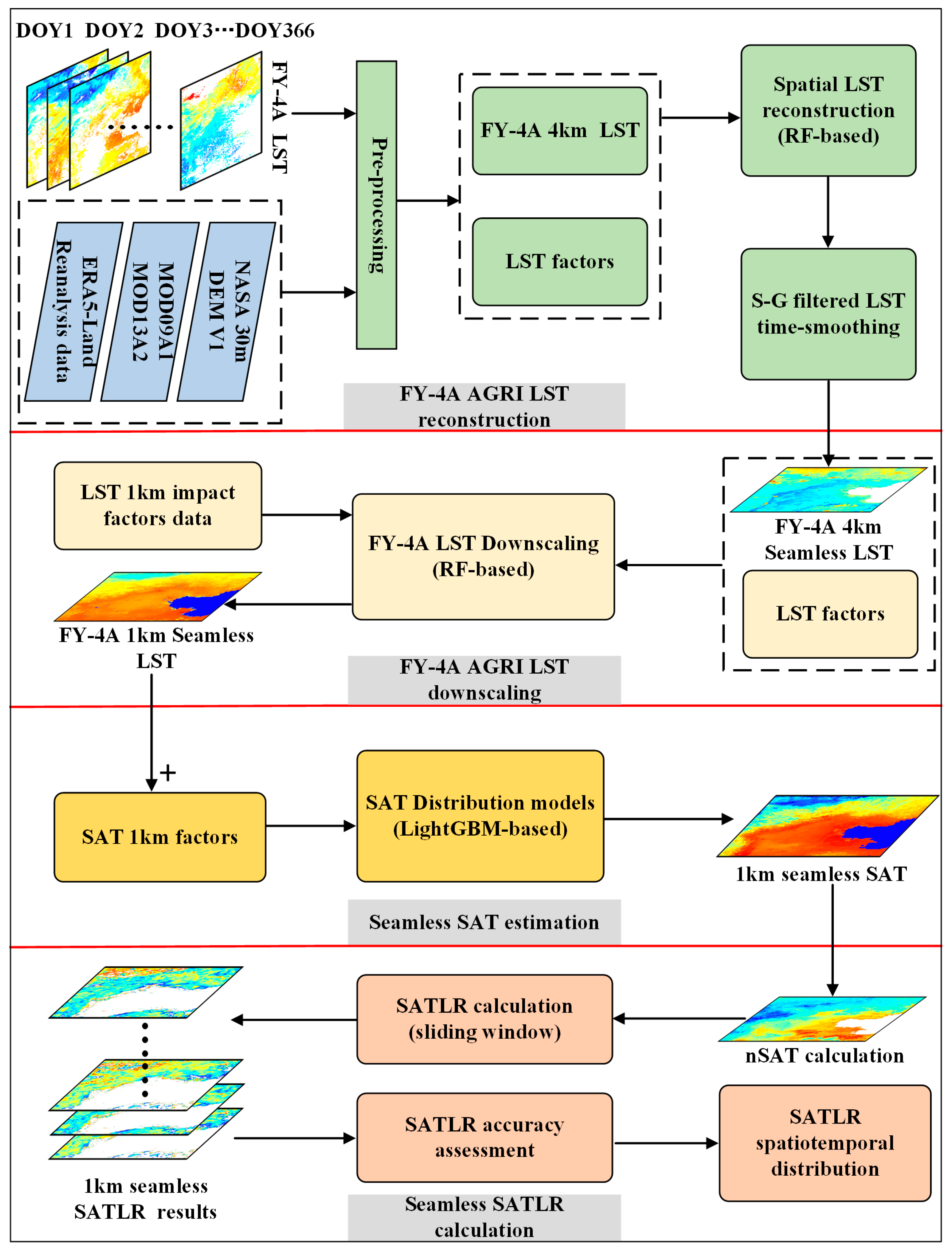
The flowchart of this study is shown in Figure 2.

2.3.1. AGRI LST Reconstruction

The AGRI LST image requires reconstruction due to weather-related missing pixels. This study employs a random forest regression model to characterize the nonlinear correlation between LST and various influencing factors, thereby establishing a spatial dimension reconstruction model for LST.
The random forest downscaling method is rooted in Breiman’s ensemble learning framework [16], which enables hierarchical modeling of spatial data through the creation of multiple classification and regression decision trees known as CART. CART operates by initially extracting several training subsets from the original low-resolution data using bootstrap resampling. Each subset then independently generates a CART decision tree, and the resulting prediction outputs from all decision trees are aggregated as high-resolution target values through weighted averaging. Within the construction of a single decision tree, random forest introduces dual sources of randomness: firstly, a set of m variables is randomly chosen from the original features as candidates for node splitting (typically with m ≈ M, where M represents the total number of features); secondly, the optimal split point is determined by minimizing the mean square error (MSE). This approach effectively enhances the model’s generalization capability. The out-of-bag data (OOB) serves as a natural validation set, with its error (EOOB) computed to assess real-time model performance. Key parameters encompass the quantity of decision trees (typically set at 500–1000) and the number of preselected variables for nodes, which are globally optimized through a random search algorithm [17]. In the specific study, the key parameters are jointly optimized by grid search and cross-validation: the number of decision trees (ntree) is determined based on the OOB error convergence, and the OOB error tends to be stable when the ntree is increased to 500, so it is set as the default value; the feature subset size (mtry) is selected by traversing the interval of [1, M] in order to minimize the RMSE of validation set, and m t r y = M is finally selected; the OOB error threshold is set to 0.5 °C, and the training is terminated early if the OOB error fluctuation of 10 consecutive iterations is less than the threshold. The ultimate model accomplishes LST reconstruction by integrating nonlinear relationships among multi-scale geographic features (e.g., elevation, vegetation index, surface reflectivity) and low-resolution temperature data.
The LST of a clear sky pixel from the FY-4A satellite is considered the dependent variable under a spatial resolution of 4 km. The independent variables include surface cumulative net radiation flux, digital elevation model (DEM), slope, normalized difference vegetation index (NDVI) and normalized difference water index (NDWI) at the pixel’s location [18]. A reconstruction model is developed using the random forest regression algorithm to establish a nonlinear regression relationship between the LST and the aforementioned independent variables [19]:
L S T = f ( S N R , N D V I , N D W I , D E M , S l o p e )
where LST stands for land surface temperature, SNR stands for surface cumulative net radiative flux, NDVI stands for normalized difference vegetation index, NDWI stands for normalized difference water body index, DEM stands for surface elevation, Slope stands for surface slope, and f stands for random forest regression model.
Following the training of the LST spatial dimension reconstruction model, the model incorporates accumulated net radiation flux, altitude, slope, NDVI, and NDWI values corresponding to the obscured pixels of LST due to cloud cover as independent variables. Subsequently, it calculates the LST beneath the clouds to fill in the missing values. SNR comprises two components, namely, SNTR and SSR, directly indicating real-time variations in the surface energy budget. Cloud cover leads to a reduction in incident SNSR due to partial blockage by clouds and an increase in downward long-wave radiation, influencing SNTR. Hence, SNR offers a comprehensive representation of the actual adjustment of cloud radiation balance. Despite the random forest model being trained on LST and SNR values from clear sky pixels, it establishes a physical relationship between clear sky conditions and LST under cloud cover by considering the impact of cloud radiation as reflected in SNR, which inherently encapsulates the dynamic cloud energy effects. By inputting the SNR of cloud-covered pixels, the model captures the specific influence of clouds on surface energy, enabling accurate prediction of the true LST beneath the clouds [20].
The LST reconstruction using the random forest algorithm is a method that operates in space dimensions. While this technique can fill in missing values, it focuses solely on the spatial distribution characteristics of LST, neglecting its temporal variations. Consequently, ensuring the temporal continuity and variability of the reconstructed LST proves challenging. To accurately represent LST under cloudy conditions, the initial LST reconstruction results must undergo temporal smoothing to address spatial reconstruction outliers. The Savitzky–Golay (S-G) filter, a method based on local polynomial least squares fitting in the time domain [21], is employed for this purpose. Statistical analysis of the reconstructed LST in the time domain followed by S-G filtering helps maintain the original shape of the LST time series while eliminating noise [20]. The S-G filtering process is mathematically described by Equation (2):
L S T j * = i = m m   C i L S T i + j N
where L S T j * is the smoothed LST reconstructed dataset, L S T i + j is the reconstructed LST data, C i is the filter coefficient, N is the number of data in the sliding window (2 m + 1) and m is the window width.

2.3.2. LST Downscaling

The reconstructed FY-4A LST has insufficient spatial resolution to fulfill the high spatiotemporal resolution demands of SATLR estimation. Therefore, downscaling the reconstructed LST is essential. Statistical downscaling methods operate under the assumption that the relationship between LST and explanatory variables remains consistent across various spatial scales at different resolutions [22].
The spatial distribution of LST in complex terrain areas is influenced by multiple factors categorized into three levels. The first level comprises large-scale geographical elements, such as altitude gradient, geographical coordinates, climate patterns, and mountainous features. The second level includes topographic micro-environment elements like surface slope, aspect, and terrain shading. The third level involves surface cover elements, such as soil properties and vegetation coverage. Given the significant topographic variability in the study area, variations in solar short-wave radiation and surface long-wave radiation exhibit notable differences [23]. Consequently, the random forest downscaling model developed in this study incorporates various factors, including LST, solar radiation, surface albedo, slope, aspect, topographic position index (TPI), NDVI, DEM and the collective impact of elevation parameters on LST. The model is trained using a low-resolution (4 km) surface parameter dataset and corresponding AGRI LST data. Subsequently, the model is applied to 1 km resolution surface parameters to generate 1 km resolution LST data through a “constant scale relationship” principle.
The main driving factors affecting the spatial distribution of LST in complex terrain regions can be divided into three levels: the first level is large-scale geographic factors, covering regional control factors such as elevation gradient, geographic coordinates, climatic background field and macro-trend of mountain ranges; the second level is the topographic micro-environmental factors, including geomorphological parameters such as surface gradient, slope direction, and terrain shading; and the third level involves the surface cover factors, such as soil properties, vegetation cover and other subsurface features, properties, vegetation cover and other subsurface characteristics. In this study area, there are significant differences in the spatiotemporal distributions of solar shortwave radiation and surface longwave radiation due to the significant topographic relief [23]; therefore, in constructing the downscaling model of random forests, this study considered the combined effects of LST and solar radiation (SR), Albedo, Slope, Aspect, TPI, NDVI and DEM, as well as the effects of elevation parameters on the LST. In the specific implementation process, the low-resolution (4 km) surface parameter dataset and the corresponding AGRI LST are firstly used to train the random forest algorithm, then the 1 km resolution surface parameters are inputted into the constructed model, and the 1 km resolution LST data are generated according to the principle of “scale relationship invariance”.

2.3.3. Remote Sensing Estimation of Spatial Distribution of Air Temperature

The spatial distribution of air temperature data is the basis for estimating the spatial distribution of SATLR. In this study, the LightGBM algorithm is used to train the air temperature spatial distribution estimation model. The LightGBM algorithm is based on the gradient boosting framework proposed by Ke et al. [24], which realizes the parallel learning of spatial features by constructing multiple decision trees based on histograms. The principle is to use the gradient one-sided sampling technique (GOSS) to screen the high error samples, and at the same time combine with the mutually exclusive feature bundle (EFB) to optimize the feature space, and each iteration round generates a new decision tree, and finally outputs the spatial air temperature distribution from the prediction results of all the trees by weighted superposition. During the construction of a single decision tree, LightGBM adopts a depth-constrained leaf-wise growth strategy; on the one hand, it avoids overfitting through the deepest constraint, and on the other hand, it selects the optimal splitting point by minimizing the weighted variance gain, which significantly improves the computational efficiency. For small sample modeling, the algorithm has built-in automatic coding of category features and missing value processing module, and dynamically monitors the mean square error (MSE) of the validation set to optimize the number of iterations through early stopping. In the spatialization of geothermal temperatures, in order to solve the challenge of high feature dimensions and sparse samples, the algorithm adopts a stratified sampling strategy to expand the training data, and sets the minimum data partitioning amount (min_data_in_leaf) greater than 20 to ensure statistical significance. The key parameters include learning rate, leaf_num and tree depth (max_depth), and hyperparameter tuning is performed by Bayesian optimization algorithm [25]. Key parameters were empirically determined for the model training process in this study. The learning rate was set at 0.05 to strike a balance between convergence speed and accuracy. The number of leaves was established at 31 to regulate model complexity. The tree depth was optimized using the Leaf-wise strategy by default. The model was trained with 100 estimators (n_estimators = 100) and a specific random seed (random_state = 42) to guarantee the reproducibility of results. A Bayesian optimization framework is utilized for hyperparameter optimization by establishing a mapping between the parameter space and validation loss using a Gaussian process surrogate model. The acquisition function, Expected Improvement, is adaptively tuned over 50 iterations to effectively trade off exploration and exploitation. This approach enhances efficiency by over 5 times compared to grid search.
The study utilized various influencing factors including station air temperature, LST, NDVI, NDWI, Albedo, SR, DEM, Slope, Aspect and TPI as training datasets. A LightGBM model was employed to establish the relationship model between 2 m SAT and influencing factors. Subsequently, the trained model was utilized to predict the air temperature for each pixel, resulting in a seamless spatial distribution of air temperature at a resolution of 1 km.

2.3.4. Estimation of the Spatial Distribution of SATLRs

1.
Calculation of nSAT using machine learning to separate the effects of elevation on air temperature
Previous research [25,26] has indicated that surface biophysical characteristics such as SSR, DEM, Slope, topographic position index (TPI), and vegetation indices like normalized difference vegetation index (NDVI), Albedo, and normalized difference water index (NDWI) influence SAT. Therefore, this study employed the LightGBM algorithm to standardize SAT, mitigating the influence of factors beyond altitude on SAT [27]. Initially, a random forest model is developed to explore the relationship between SAT and various influencing factors:
S A T = g ( D E M , N D V I , N D W I , A l b e d o , S S R , S l o p e , A s p e c t , T P I )
where SAT is the near-surface 2 m air temperature distribution obtained in Section 2.3.3 and g is the nonlinear connectivity modeled using the LightGBM algorithm (mentioned in Section 2.3.3).
Separating the influence of influence parameters other than DEM on SAT to obtain nSAT:
S A T m = h ( N D V I , N D W I , A l b e d o , S S R , S l o p e , A s p e c t , T P I )
n S A T = S A T S A T m
In Equations (4) and (5), SATm is SAT model based on influencing factors other than DEM surface features, nSAT is normalized SAT, and h is nonlinear relationship model.
2.
Estimation of SATLR on the basis of nSAT using the sliding window method
In view of the reliability characteristics of TLR at local scales, most of the existing studies adopt the gridded method for spatial analysis, in which some scholars realize the TLR calculation by extracting the local sample data within the grid cells [5,15]. In this study, the sliding window method is adopted by fitting a linear regression equation between nSAT and elevation data in the window coverage area, and defining the coefficient a of the regression equation as the SATLR, for the image element at the center of this window:
n S A T = a × D E M + b
where nSAT is the normalized near-surface air temperature of each pixel within the sliding window, DEM is the altitude of the corresponding pixel and a and b are regression coefficients.
To enhance the precision of SATLR data computation, specific criteria are applied to identify pixels suitable for the linear regression model. The linear regression calculation within the sliding window is executed only when the elevation span of nSAT pixels in the window (defined as the difference between the highest and lowest altitudes) exceeds 10 m [2,27,28]. If the altitude differential falls below this threshold, the TLR value of the central grid is designated as null. Additionally, any computed values outside the range of −10 ≤ SATLR < 15 °C/km are deemed unreliable, leading to the exclusion of the corresponding pixel [2]. The size of the sliding window incrementally expands from 5 × 5 until the model satisfies the significance test at a 95% confidence level.

2.3.5. SATLR Estimation Accuracy Assessment

Due to the limited station density, it is unfeasible to compute the SATLR using the sliding window technique and subsequently assess the spatial distribution of the SATLR as estimated by this method. In this investigation, two station pairs situated 5–10 km apart with an altitude variance exceeding 400 m were chosen [1,2], and the ratio of air temperature discrepancy to altitude variance was regarded as the observed metric. The coefficient of determination (R2), mean absolute error (MAE) and RMSE served as metrics for accuracy assessment in appraising the precision of the air temperature difference to altitude difference ratio estimated by the two station pairs.

3. Result

3.1. Feasibility Analysis of SATLR Spatial Distribution Calculation Based on Air Temperature Estimation from Remote Sensing

The ratio of the 2 m air temperature difference to the elevation difference observed at the two eligible stations was used as the observed value to assess the accuracy of the nSAT difference to elevation difference ratio estimated at the two station locations, and the results are shown in Table 1, featuring columns for time, R2, RMSE, MAE and N (representing the sample size for site pairs). The error metrics, RMSE and MAE, are denoted in degrees Celsius, whereas R2 and N are dimensionless parameters.
These site pairs encompass diverse terrains and land use types, with elevations ranging from 0.5 m to 2422 m, slopes ranging from 0° to 38.83° and slope directions spanning from 0° to 358.72°. The land use types comprise cropland, grassland, impervious, forest, shrub and water, effectively capturing the fundamental surface characteristics of the region. Due to the exhaustive utilization of all eligible station pairs, abundant sampling data, and high spatial representativeness, the verification outcomes exhibit a high level of reliability.
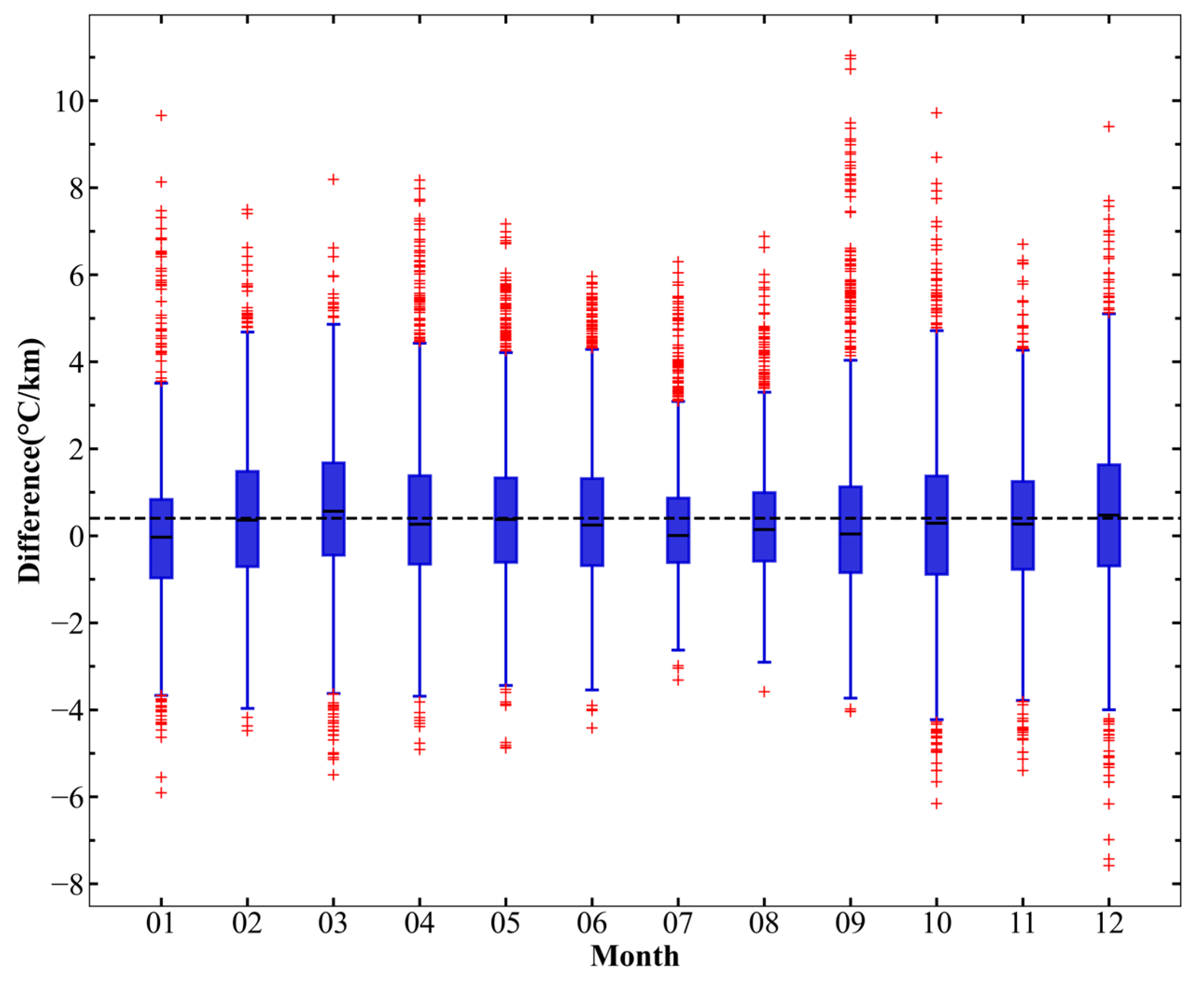
Further, in this study, the degree of deviation between the observed and estimated values of SATLR was quantified by constructing difference box-and-line plots (as shown in Figure 3). In Figure 3, the box is represented by a blue rectangle, with its upper and lower edges corresponding to the 25% and 75% quartiles, the ends of the upper and lower whisker lines extending from the box correspond to the 2.5% and 97.5% quartiles and the outliers are marked with red plus signs on the outside of the whisker lines. In this case, the box region between the upper and lower edges (i.e., the first quartile Q1 and the third quartile Q3) represents the distribution of the middle 50% of the data; the end of the upper and lower whisker lines (i.e., the 2.5% and 97.5% quartiles) defines the total range that contains the 95% of the data, which means that the vast majority of the data points fall within this interval; and the red plus sign on the outer whisker line represents the 95% of values that fall outside of this 95% range of extreme values, i.e., outliers. According to Figure 3, 95% of the meteorological stations have a SATLR of no more than ±4 °C/km, with half of the stations controlled within ±1 °C/km. Considering the significant spatial variability of the SATLR itself, the above deviation is at a relatively low level, which fully proves that the air temperature spatial distribution model constructed in this paper has good generalization ability and regional adaptability.
Based on the comprehensive analysis of the above Table 1 and Figure 3, it can be seen that the SATLR estimated by using the method of air temperature difference and elevation difference between station pairs is more accurate, and it also indirectly shows that the sliding window method can reliably estimate the spatial distribution of the SATLR with a high degree of accuracy.

3.2. Characterization of the Spatiotemporal Distribution of the Annual Average SATLR

This study adheres to the standard practice in atmospheric science, where positive values denote a decrease in air temperature with altitude, while negative values signify an increase in air temperature with altitude [6]. Additionally, positive SATLR values are referred to as steep, whereas negative values are characterized as shallow.
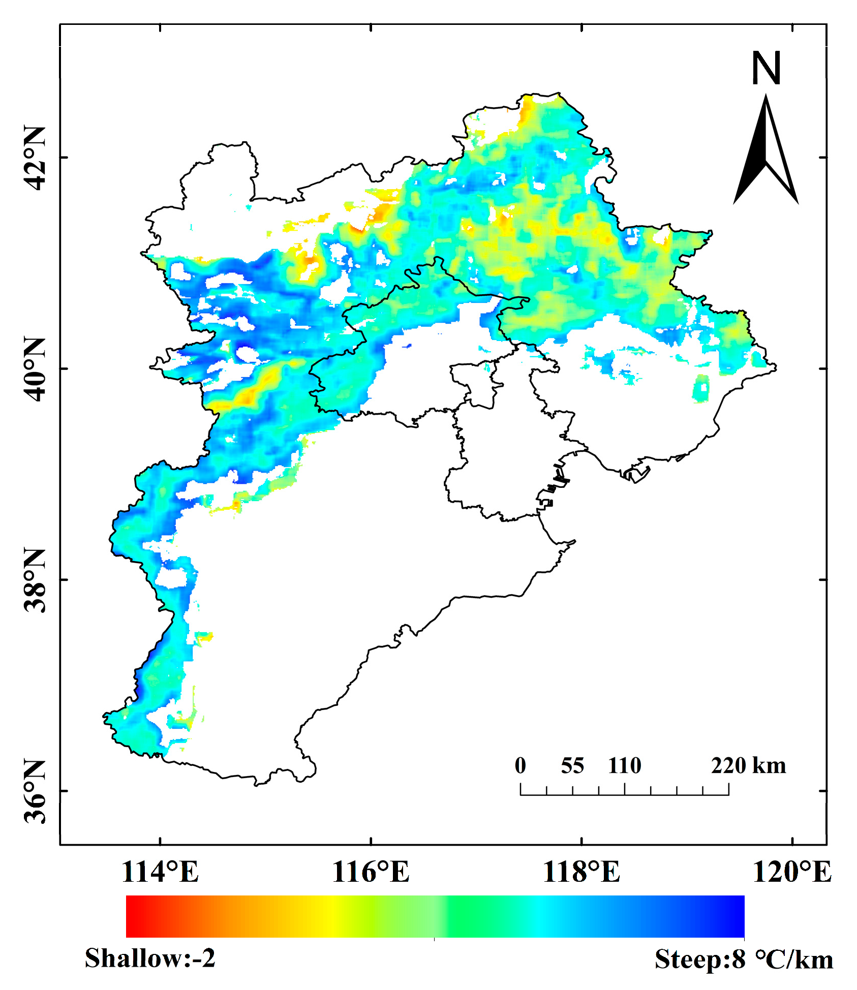
The spatial distribution of annual SATLR in the study area is illustrated in Figure 4, indicating that the annual average SATLR predominantly ranges between 2~6 °C/km. Deeper SATLR values (>6 °C/km) are primarily concentrated in the Taihang Mountains area in the southwest, the Huapiling area of Damaquan Mountain in the northwest, and certain regions of Beijing City in the central area. This may be due to the western foothills of the Taihang Mountains being located on the leeward slope of the southeast monsoon, where significant downward airflow warming (the burning wind effect) results in high valley bottom temperatures, increasing the temperature difference with high-altitude areas. Dama Qunshan lies in the main channel of winter winds, where cold air sinking down the slope exacerbates cooling in low-altitude areas, while solar radiation heating is more pronounced at high altitudes, expanding the vertical temperature difference [29]. Moreover, SATLR exceeding 7 °C/km is observed in specific areas in the southwest of Zhangjiakou City and at the southern foothills of Yanshan Mountains. Conversely, areas exhibiting shallow SATLR values (<2 °C/km) are predominantly situated in Chengde City in the northeast, as well as on the northern and southern flanks of Huapiling Mountain in Damaqun Mountains to the northwest. Additionally, SATLR values shallower than 0 °C/km are evident in select areas northeast of Zhangjiakou City. This may be because Chengde is situated within the hinterland of the Yanshan Mountains, where the uplift of southeastern monsoon winds on windward slopes induces rainfall. Increased cloudiness weakens solar radiation, reducing the temperature difference between high and low altitudes. Additionally, cold air accumulates at the northern foot of the Yanshan Mountains during winter, forming a stable inversion layer that inhibits the decrease in temperature with altitude.
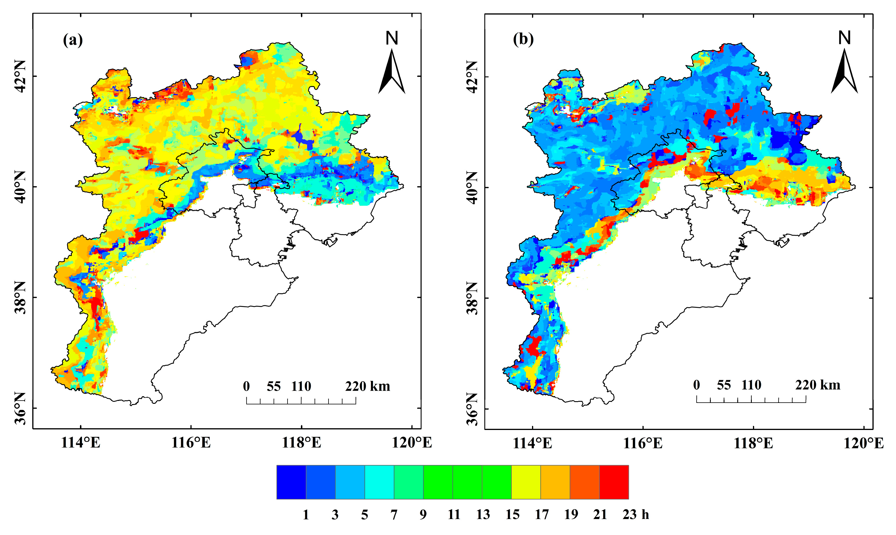
The moments when the annual mean SATLR reaches its steepest value (a) and shallowest value (b) are shown in Figure 5. According to Figure 5, the annual mean SATLR in the study area generally reaches its shallowest value from 5:00 to 9:00 p.m. and its steepest value from 12:00 to 15:00 p.m.
Figure 6 illustrates the annual variation in SATLR, defined as the disparity between the highest and lowest monthly average SATLR within a year. The data reveals that in the BTH mountainous region, most areas exhibit an annual SATLR range of 3~5 °C/km. Regions with a larger annual range (>5 °C/km) are predominantly found in the northern Yanshan Mountains, Damaqun Mountains, foothills of Taihang Mountains, Tangshan City and Qinhuangdao City, consistent with Qin’s findings. Conversely, areas with a smaller annual range (<3 °C/km) are primarily located in the Taihang Mountains ridge, southern Chengde City, western Beijing City and southern Yanshan Mountains.
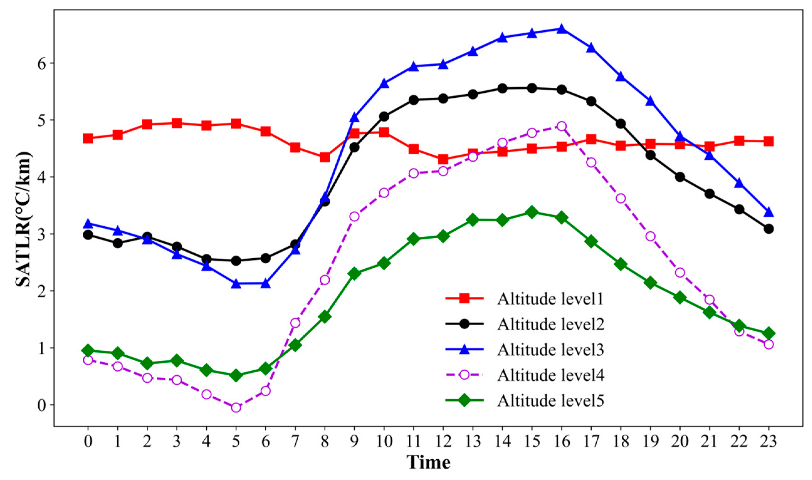
The substantial variability in SATLR across different altitudes underscores the importance of examining its spatiotemporal fluctuations to elucidate vertical climate gradients. Such analysis not only enhances the precision of regional climate models, but also provides crucial data for ecological conservation, agricultural planning and hydrological resource management in mountainous regions. In this investigation, the study area’s altitude was categorized into five tiers: below 500 m, 500–1000 m, 1000–1500 m, 1500–2000 m and above 2000 m. SATLR values for all valid pixels within each tier were averaged to represent the SATLR at each time point. Subsequently, annual SATLR variations were computed for each tier, as depicted in Figure 7.
Figure 7 illustrates significant temporal variations in the SATLR at different altitudes within the study area. Throughout the day, SATLR trends in the second to fifth altitude grades exhibit similarity, albeit with varying overall values. The SATLR typically reaches its deepest between 14:00 and 16:00, its shallowest between 5:00 and 6:00, and experiences a notable increase between 6:00 and 9:00. Specifically, the third altitude level demonstrates the deepest overall SATLR values, ranging from 2 °C/km to 7 °C/km. In contrast, the fifth altitude level exhibits the shallowest SATLR values, ranging from 0 °C/km to 3 °C/km. The second and fourth altitude levels display intermediate SATLR values, ranging from 2 °C/km to 6 °C/km and from −1 °C/km to 5 °C/km, respectively. At the lowest first altitude level, the SATLR values remain relatively stable throughout the day, maintaining a range of 4 °C/km to 5 °C/km.
Figure 7 illustrates that the SATLR typically reaches its deepest during the midday to afternoon period and its shallowest around dawn, sunrise, or in the morning under local inversion conditions (e.g., at the fourth altitude). As air temperatures decrease at night, the air’s moisture content rises, leading to the condensation of water vapor in the atmosphere into minute droplets. This increased humidity results in a more stable thermodynamic structure of the atmosphere, characterized by a reduction in the air temperature gradient per unit height. The distinct thermodynamic processes between daytime and nighttime contribute to the shallower SATLR during nighttime compared to daytime [2], particularly reaching its shallowest point from early morning to predawn, and temperature inversions potentially occurring.
Temperature inversions are common meteorological occurrences in mountainous regions [30], primarily driven by surface radiation cooling during cloudless nights. As the surface cools, the adjacent air also cools, causing cold air at higher altitudes to descend along the slopes, forming a cold pool due to the terrain configuration. Research by Clements et al. demonstrated that valley wind circulation initiates downslope density flow, transporting cold air and leading to warm air subsidence to maintain stable stratification. This process results in increasing temperatures with height, ultimately forming a radiation inversion [31], aligning with the observations in the current study.

3.3. Characterization of the Spatio-Temporal Distribution of SATLR Across Seasons

Figure 8 demonstrates the seasonal average SATLR. The data depicted in Figure 8 indicates that SATLR values during spring, summer and autumn predominantly range between 3 and 5 °C/km, whereas in winter, SATLR values are comparatively shallower, with a broader distribution between 2 and 4 °C/km. The spatial distribution of SATLR across different seasons mirrors that of the annual SATLR. In the northern region of the study area, notable temperature inversions are evident during winter in various areas of the Damaqun Mountains and sporadically in the Taihang Mountains. Additionally, temperature inversions occur in select areas of the Damaqun Mountains and Taihang Mountains during other seasons.
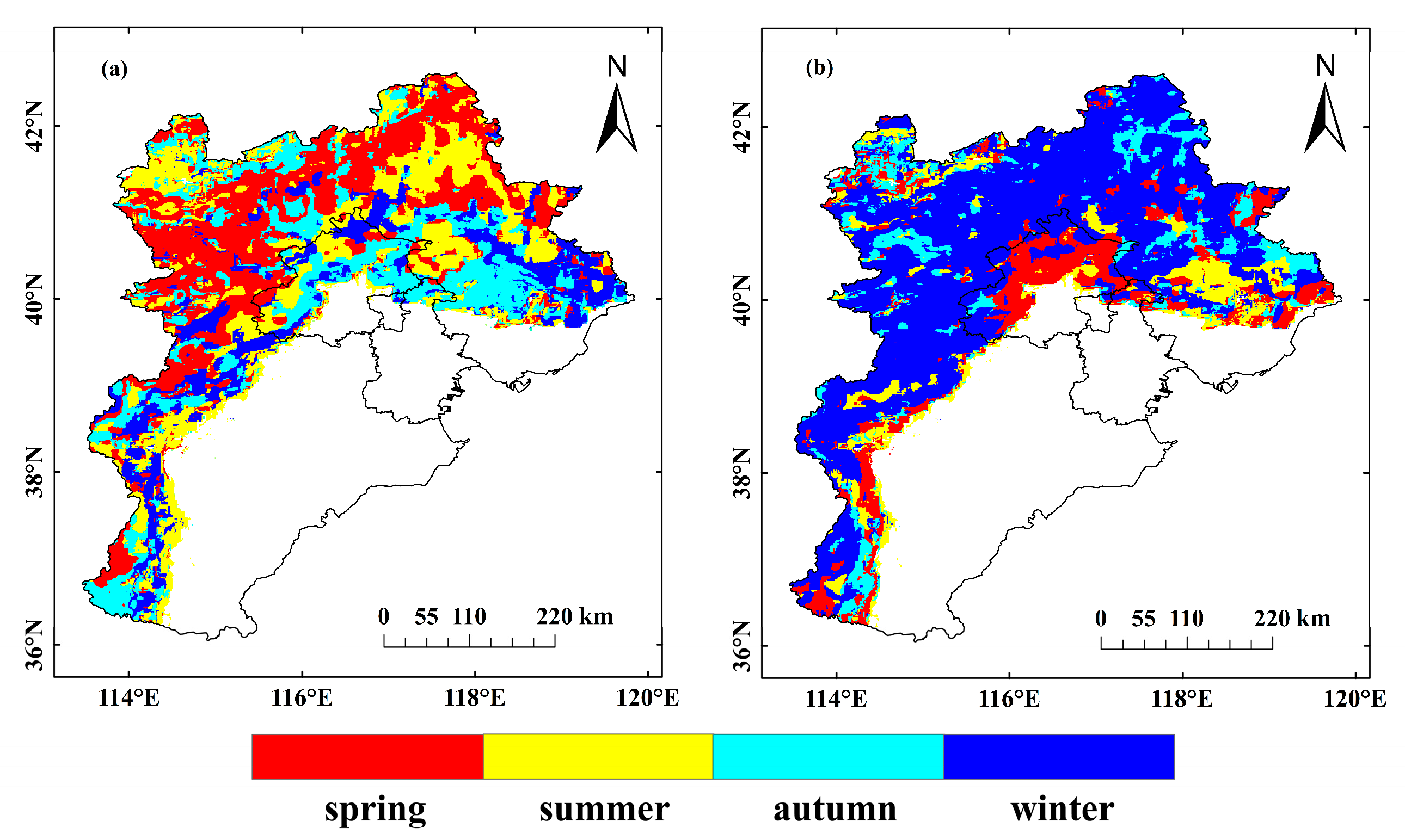
Figure 9 presents the seasonal variations in the monthly mean SATLR, depicting its steepest (a) and shallowest (b) values. The data reveals that, generally, the SATLR is most pronounced in spring, followed by summer and autumn, with the shallowest values observed during winter. Specifically, the deepest monthly SATLR occurs in summer in certain regions of Chengde City in the northeast and the north of Damaquan Mountains in the northwest of the study area. In contrast, the deepest SATLR is observed in autumn in the northern Yanshan Mountains area and some parts of the Taihang Mountains, while winter marks the period with the deepest overall SATLR. The shallowest monthly SATLR predominantly manifests in winter, except for the southern Yanshan Mountains and the Taihang Mountains foothills where it occurs in summer. Additionally, in some areas such as the southern Yanshan Mountains and eastern Taihang Mountains, the shallowest SATLR is observed in spring, while autumn records the shallowest values in the northern and southern slopes of Damaqun Mountains and parts of the northern Yanshan Mountains within Chengde City.
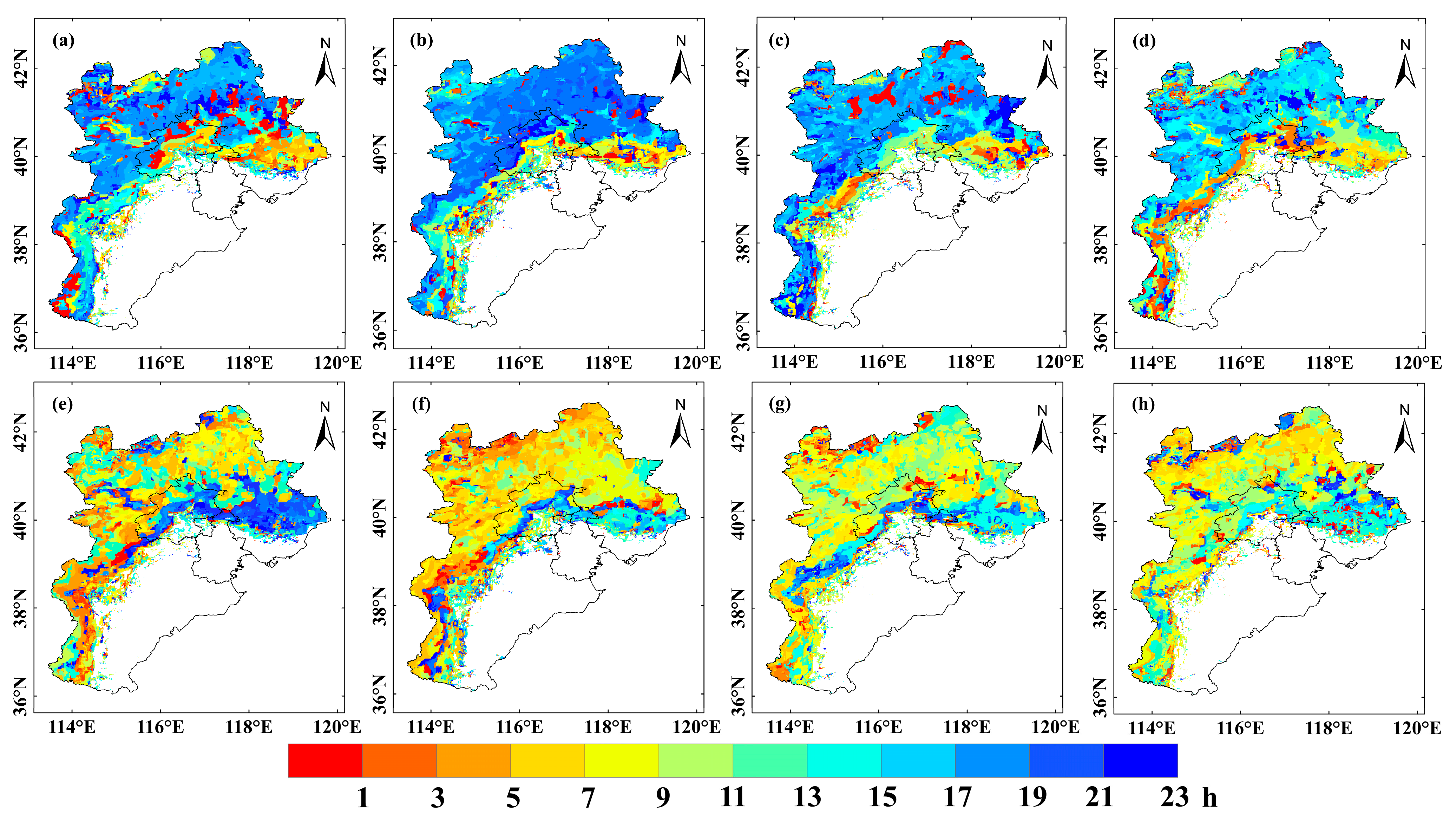
Figure 10 shows the timing of the seasonal deepest and shallowest values of the average SATLR. The data indicates that, in comparison to the yearly average SATLR, the shallowest values typically occur between 5:00 and 9:00. Specifically, during summer in many regions of the study area, this shallowest time shifts earlier to 4:00 to 6:00, while in spring, areas such as Tianshan Mountain and neighboring regions in northwest China experience a delay to 7:00 to 10:00. This temporal shift, characterized by both advancement and delay, appears to be influenced by variations in sunrise times. In summer, with the direct sunlight on the northern hemisphere leading to earlier sunrises, the timing of the shallowest SATLR values advances. Conversely, in winter, the later sunrise times result in a delayed occurrence of the shallowest SATLR values.
In contrast to the seasonal fluctuation pattern of the SATLR, the pattern of the deepest SATLR in the research area indicated an earlier onset in spring compared to the annual average, a lag in autumn and values close to the annual average in summer and winter. This phenomenon can be attributed to several factors. During spring, the gradual increase in solar radiation leads to rapid surface heating, which accelerates the dissipation of the near-surface inversion layer and weakens the mountain terrain’s cold air blocking effect, thereby advancing the peak of vertical atmospheric instability. In summer, the peak solar radiation intensity and reduced day–night temperature difference hinder the persistence of the inversion layer. In winter, the combination of minimal solar radiation and the accumulation of cold air due to topography maintains a stable temperature vertical gradient, resulting in an average SATLR. Thus, the spatiotemporal variability of SATLR primarily arises from the seasonal changes in solar radiation and the interaction between topography and the atmosphere.
In addition, this study plots seasonal mean hourly SATLR curves, as shown in Figure 11.
Figure 11 illustrates notable temporal variability of SATLR across varying altitudes and seasons in the research area. Consistent with the annual patterns of SATLR across altitudes, the trends in SATLR for grades two through five exhibited similarity across seasons. However, the overall levels of SATLR varied across altitudes in different seasons, with distinct patterns observed for the first grade of SATLR in each season.
In contrast to the temporal variability of SATLR across the year, the deepest SATLR values across all altitude levels generally occur between 17:00 and 19:00 in spring, with a peak observed from 9:00 to 10:00. Conversely, the shallowest average SATLR values in spring typically occur from 5:00 to 6:00, accompanied by a pronounced increase in slope between 5:00 and 9:00. Notably, the diurnal pattern of SATLR in the first altitude level exhibits an opposite trend compared to other levels, with deeper values at night and shallower values during the day, lacking distinct peak and valley values and displaying a noticeable decrease in slope from 5:00 to 8:00. Consistent with the annual trends observed for SATLR across different altitudes, the deepest overall SATLR occurs at the third altitude level, while the shallowest is recorded at the fifth altitude level. However, unlike the annual SATLR patterns across altitude levels, the second and fourth altitude levels exhibit comparable intermediate SATLR values, with overlapping curves between 7:00 and 19:00. Nevertheless, the SATLR values at the second level are notably higher than those at the fourth level during other time periods.
In summer, the SATLR typically reaches its deepest between 16:00 and 18:00 and its shallowest between 4:00 and 5:00 across all altitudes. Unlike other seasons, in summer, the SATLR exhibits a gradual increase rather than a sharp incline around sunrise. The overall magnitude of SATLR across varying altitudes remains relatively stable compared to the annual average level.
During autumn, the SATLR exhibits its deepest between 14:00 and 16:00, reaching its shallowest around 6:00, and displaying a sharp increase between 6:00 and 9:00. The vertical distribution of SATLR across different altitude levels generally aligns with the annual average pattern. Notably, akin to the spring season, minor peaks are observed between 9:00 and 10:00 at the fourth and fifth altitude levels, with temperature inversions occurring at the fourth level between 4:00 and 6:00 before sunrise. Furthermore, in the lowest altitude region, there is a slightly amplified fluctuation in SATLR compared to the annual average curve, peaking at 9:00 and reaching its shallowest point at 13:00. Despite this variation, SATLR remains relatively stable in comparison to higher altitude regions.
In winter, the diurnal variation in the SATLR exhibited a distinct pattern compared to autumn. Specifically, the peak SATLR values across all altitudes coincided with those observed in autumn, but the overall increase in SATLR exhibited a delayed “steep slope” between 7:00 and 10:00. Between 11:00 and 16:00, SATLR curves converged across altitudes without significant variation, while in other time intervals, a trend emerged where higher altitudes corresponded to shallower SATLRs, except for the fourth and fifth altitude grades, which displayed an opposite trend. Notably, the SATLR curve at the lowest altitude level closely resembled the annual average, displaying minimal overall variability. The inversion phenomenon was more pronounced in winter than in autumn, particularly evident in the fourth and fifth altitude grades from early morning until sunrise, with the fourth grade exhibiting a shallower SATLR by approximately 1 °C/km compared to the fifth grade during this period.

4. Discussion

4.1. Advantages

To address the challenge that satellite remote sensors cannot acquire SATLRs with high spatiotemporal resolution, and considering the unclear various characteristics of hourly SATLR across different geographical positions, this paper proposes an effective spatiotemporal resolution method for estimating SATLR. This method utilizes FY-4A AGRI LST data with high temporal resolution. Based on reconstructed FY-4A AGRI LST data, this study downscales the 4 km resolution data to 1 km resolution using machine learning. It then estimates the spatial distribution of SAT and nSAT by integrating station observations. Subsequently, hourly SATLR distribution at the resolution of 1 km are estimated. The method proposed maximizes the benefits of integrating remote sensing imagery with station observation data to accurately estimate the SATLR at a high spatiotemporal resolution.
Simultaneously, the method proposed in this study is applicable to regions with surface temperature and station-measured air temperature data. It can be used to spatially estimate SATLR distribution in other mountainous systems around the world by combining land surface temperature, terrain parameters, and station observation air temperature data using the sliding window method.

4.2. Disadvantages

Although the proposed method estimates SATLR with high spatial and temporal resolution, it still has some limitations. First, errors introduced during SATLR estimation propagate through multiple stages. In the LST reconstruction phase, the nonlinear relationship model built using clear-sky pixels inherently contains errors. While the model incorporates net radiation flux parameters to account for cloud-cover differences when applied to cloudy pixels, applying a model established under clear-sky conditions to cloud-covered areas inevitably introduces additional errors of approximately 1–2 K. During the downscaling phase, the machine learning model fails to fully capture the complex relationship between LST and its influencing factors. Furthermore, the simplification process, which assumes invariance across scales, introduces additional errors of about 1.5 K. SAT estimation error, primarily stemming from the machine learning model’s inherent uncertainty, is around 1 K. When calculating SATLR within a sliding window, the estimation accuracy is influenced by both the window size and the regional elevation difference. Due to the lack of true SATLR reference data, the calculated value of SATLR cannot be compared with the reference value, so the ratio of 2 m temperature difference and altitude difference observed at two stations meeting the conditions is taken as the observed value to evaluate the accuracy of the estimated value of nSAT difference and altitude difference ratio of two stations. Notably, the aforementioned errors exhibit nonlinear relationships, the total error is not a simple linear accumulation of the errors from each individual step.
In reconstructing LST, a random forest model is employed to fill gaps caused by cloud cover. However, during prolonged rainy periods that extensively and continuously cover the entire study area, the lack of clear-sky pixels prevents effective spatial reconstruction of missing LST data due to insufficient training data for the model.
This study analyzed the spatiotemporal patterns of SATLRs using only the 2020 monthly time-series data for the study area, focusing on monthly and seasonal variations. It did not investigate the multi-year trends or the spatiotemporal characteristics of SATLR under extreme climate conditions. Consequently, further research is necessary to understand the interannual variability of SATLR and its spatial and temporal distribution patterns during extreme climatic events.

5. Conclusions

SATLR plays a crucial role in assessing atmospheric stability, validating climate models, and supporting hydroecological research. However, obtaining high-resolution SATLR data in complex terrain regions is challenging due to various limitations. To address this issue, this study introduces a novel approach for estimating SATLRs at high spatiotemporal resolution. This method involves downscaling FY-4A AGRI LST data, which offers high temporal resolution, to a 1 km scale using reconstructed LST data. Subsequently, SATs are estimated through LightGBM, enabling the calculation of high-resolution SATLR.
Utilizing the aforementioned methodologies, the 2020 hourly AGRI LST data was employed to assess the temporal and spatial variation characteristics of SATLR in the mountainous region of BTH. The key findings are as follows: firstly, the average annual SATLR ranges predominantly between 2 and 6 °C/km across the BTH mountainous area, with instances of SATLR exceeding 6 °C/km observed in the Taihang Mountains region to the southwest, the Huapiling area of Damaquan Mountain to the northwest, and certain parts of Beijing, while reaching 7~13 °C/km in select areas southwest of Zhangjiakou City. Conversely, SATLR below 2 °C/km was noted in Chengde City to the northeast and in the northern and southern regions of Huapiling in Damaquan Mountain to the northwest, with SATLR below 0 °C/km recorded in specific areas northeast of Zhangjiakou City. Moreover, the seasonal spatial distribution of SATLR in the BTH mountainous area exhibited similarities to the annual averages. Notably, during winter, pronounced inversion phenomena were evident in numerous areas of Damaqun Mountains and some regions of Taihang Mountains to the north, with isolated occurrences of temperature inversions in both Damaqun Mountains and Taihang Mountains during other seasons. In addition, the diurnal variation in SATLR in various altitude zones within the BTH mountainous region indicates that SATLR typically reaches its deepest from midday to afternoon and becomes shallowest with localized temperature inversions from early morning until around sunrise or morning. Specifically, the SATLR curve at lower altitudes remains relatively stable, while the trend in other altitude zones is comparable. Furthermore, SATLR exhibits distinct patterns across different altitude zones during various seasons, notably demonstrating a consistent and pronounced temperature inversions from early morning to sunrise during winter.
This study employs a machine learning algorithm to predict high spatiotemporal resolution SATLR using high-frequency LST data. This involves reconstructing LST, downscaling LST, reconstructing SAT, and calculating nSAT. By utilizing the sliding window technique, precise SATLR parameters can be obtained for applications in hydrological, glacial and ecological modeling; regional downscaling; and the acquisition of high-resolution temperature datasets.

Author Contributions

Conceptualization, Q.L., S.Z. and G.Z.; methodology, Q.L., S.Z. and G.Z.; software, Q.L.; validation, Q.L. and Y.L.; formal analysis, Q.L.; investigation, Q.L. and Y.L.; resources, S.Z. and G.Z.; data curation, Q.L.; writing—original draft preparation, Q.L.; writing—review and editing, M.S., S.Z., and G.Z.; visualization, Q.L.; supervision, M.S., S.Z. and G.Z.; project administration, M.S., S.Z. and G.Z. All authors have read and agreed to the published version of the manuscript.

Funding

This study was funded by Fengyun Application Pioneering Project (No. FY-APP-2022.0204) and the Natural Science Foundation of China (Nos. 42171101, 42271351).

Data Availability Statement

FY-4A AGRI LST products presented in this study are openly available at https://satellite.nsmc.org.cn/portalsite/Data/Satellite.aspx, ERA5-Land reanalysis data are openly available at https://cds.climate.copernicus.eu/cdsapp#!/dataset/reanalysis-era5-land-monthly-means?tab=form (accessed on 10 April 2023), MODIS reflectance and vegetation index products are openly available at https://ladsweb.modaps.eosdis.nasa.gov/ (accessed on 10 April 2023), NASA DEM data are openly available at https://search.earthdata.nasa.gov/ (accessed on 15 April 2025), land cover data presented in this study are openly available at http://www.ncdc.ac.cn/portal/metadata/9de270f3-b5ad-4e19-afc0-2531f3977f2f (accessed on 10 April 2023).

Acknowledgments

The authors would like to thank the Feng Yun Satellite Remote Sensing Data Network, the European Center for Medium-Range Weather Forecasts and the China National Cryosphere Desert Data Center for providing data to improve this paper. The authors would also like to thank anonymous reviewers and the Editor for their valuable suggestions, which helped us to significantly improve the quality of the manuscript.

Conflicts of Interest

The authors declare no conflicts of interest; no human or animal subjects were involved in this study.

References

  1. Zhang, G.; Zhang, G.; Zhu, S.; Zhang, N.; Xu, Y. Estimation on the Hourly Distribution of Near-Surface Temperature Lapse Rate Under Winter Clear-Sky Conditions. IEEE Trans. Geosci. Remote Sens. 2023, 61, 4107013. [Google Scholar] [CrossRef]
  2. Qin, Y. The Spatiotemporal Characteristics of Temperature Lapse Rate in China. Ph.D. Thesis, China University of Geosciences, Wuhan, China, 2022. [Google Scholar]
  3. Firozjaei, M.K.; Fathololoumi, S.; Alavipanah, S.K.; Kiavarz, M.; Vaezi, A.R.; Biswas, A. A New Approach for Modeling near Surface Temperature Lapse Rate Based on Normalized Land Surface Temperature Data. Remote Sens. Environ. 2020, 242, 111746. [Google Scholar] [CrossRef]
  4. Kirchner, M.; Faus-Kessler, T.; Jakobi, G.; Leuchner, M.; Ries, L.; Scheel, H.; Suppan, P. Altitudinal Temperature Lapse Rates in an Alpine Valley: Trends and the Influence of Season and Weather Patterns. Int. J. Climatol. 2013, 33, 539–555. [Google Scholar] [CrossRef]
  5. Li, X.; Wang, L.; Chen, D.; Yang, K.; Xue, B.; Sun, L. Near-surface Air Temperature Lapse Rates in the Mainland China during 1962–2011. J. Geophys. Res. Atmos. 2013, 118, 7505–7515. [Google Scholar] [CrossRef]
  6. Shen, Y.; Shen, Y.; Goetz, J.; Brenning, A. Spatial-temporal Variation of Near-surface Temperature Lapse Rates over the Tianshan Mountains, Central Asia. J. Geophys. Res. Atmos. 2016, 121, 14-006. [Google Scholar] [CrossRef]
  7. Córdova, M.; Célleri, R.; Shellito, C.J.; Orellana-Alvear, J.; Abril, A.; Carrillo-Rojas, G. Near-Surface Air Temperature Lapse Rate Over Complex Terrain in the Southern Ecuadorian Andes: Implications for Temperature Mapping. Arct. Antarct. Alp. Res. 2016, 48, 673–684. [Google Scholar] [CrossRef]
  8. Yao, Y.; Xu, M.; Zhang, B. The Implication of Mass Elevation Effect of the Tibetan Plateau for Altitudinal Belts. J. Geogr. Sci. 2015, 25, 1411–1422. [Google Scholar] [CrossRef]
  9. Peng, S.; Piao, S.; Ciais, P.; Myneni, R.B.; Chen, A.; Chevallier, F.; Dolman, A.J.; Janssens, I.A.; Peñuelas, J.; Zhang, G.; et al. Asymmetric Effects of Daytime and Night-Time Warming on Northern Hemisphere Vegetation. Nature 2013, 501, 88–92. [Google Scholar] [CrossRef]
  10. Seguin, B. Use of Surface Temperature in Agrometeorology. In Applications of Remote Sensing to Agrometeorology; Toselli, F., Ed.; Ispra Courses; Springer Netherlands: Dordrecht, The Netherlands, 1989; pp. 221–240. ISBN 978-94-010-7501-5. [Google Scholar]
  11. Yao, Y.; Zhang, B.; Zhao, C. Geographical distribution of cripple tree forest and its importance for forest line in China. Prog. Geogr. 2017, 36, 491–499. [Google Scholar] [CrossRef]
  12. Goetz, S.J.; Prince, S.D.; Small, J. Advances in Satellite Remote Sensing of Environmental Variables for Epidemiological Applications. In Remote Sensing and Geographical Information Systems in Epidemiology; Advances in Parasitology; Academic Press: Cambridge, MA, USA, 2000; Volume 47, pp. 289–307. [Google Scholar]
  13. Vogt, J.V.; Viau, A.A.; Paquet, F. Mapping Regional Air Temperature Fields Using Satellite-Derived Surface Skin Temperatures. Int. J. Climatol. 1997, 17, 1559–1579. [Google Scholar] [CrossRef]
  14. Wang, Y.X.; Ding, K.; Huang, X.Y.; Long, X.M.; Zhou, R.L. Temperature lapse rates in the mountain regions of Yunnan Province based on remotely sensed instantaneous land surface temperature. J. Remote Sens. 2014, 18, 912–922. [Google Scholar] [CrossRef]
  15. Romshoo, S.A.; Rafiq, M.; Rashid, I. Spatio-Temporal Variation of Land Surface Temperature and Temperature Lapse Rate over Mountainous Kashmir Himalaya. J. Mt. Sci. 2018, 15, 563–576. [Google Scholar] [CrossRef]
  16. Breiman, L. Random Search. Mach. Learn. 2001, 45, 5–32. [Google Scholar] [CrossRef]
  17. Bergstra, J.; Bengio, Y. Random Search for Hyper-Parameter Optimization. J. Mach. Learn. Res. 2012, 13, 281–305. [Google Scholar]
  18. Jin, M.; Dickinson, R.E. Land Surface Skin Temperature Climatology: Benefitting from the Strengths of Satellite Observations. Environ. Res. Lett. 2010, 5, 044004. [Google Scholar] [CrossRef]
  19. Zhao, W.; Duan, S.-B. Reconstruction of Daytime Land Surface Temperatures under Cloud-Covered Conditions Using Integrated MODIS/Terra Land Products and MSG Geostationary Satellite Data. Remote Sens. Environ. 2020, 247, 111931. [Google Scholar] [CrossRef]
  20. Savitzky, A.; Golay, M.J.E. Smoothing and Differentiation of Data by Simplified Least Squares Procedures. Anal. Chem. 1964, 36, 1627–1639. [Google Scholar] [CrossRef]
  21. Li, Y.; Zhu, S.; Zhang, G.; Xu, W.; Jiang, W.; Xu, Y. Reconstruction of Hourly FY-4A AGRI Land Surface Temperature under Cloud-Covered Conditions Using a Hybrid Method Combining Spatial and Temporal Information. Remote Sens. 2024, 16, 1777. [Google Scholar] [CrossRef]
  22. Zhu, J.; Zhu, S.; Yu, F.; Zhang, G.; Xu, Y. A downscaling method for ERA5 reanalysis land surface temperature over urban and mountain areas. Natl. Remote Sens. Bull. 2021, 25, 1778–1791. [Google Scholar] [CrossRef]
  23. Hais, M.; Kučera, T. The Influence of Topography on the Forest Surface Temperature Retrieved from Landsat TM, ETM + and ASTER Thermal Channels. ISPRS J. Photogramm. Remote Sens. 2009, 64, 585–591. [Google Scholar] [CrossRef]
  24. Ke, G.; Meng, Q.; Finley, T.; Wang, T.; Chen, W.; Ma, W.; Ye, Q.; Liu, T.-Y. LightGBM: A Highly Efficient Gradient Boosting Decision Tree. In Proceedings of the 31st International Conference on Neural Information Processing Systems, Long Beach, CA, USA, 4–9 December 2017; Curran Associates Inc.: Red Hook, NY, USA, 2017; pp. 3149–3157. [Google Scholar]
  25. Snoek, J.; Larochelle, H.; Adams, R.P. Practical Bayesian Optimization of Machine Learning Algorithms. In Proceedings of the 26th International Conference on Neural Information Processing Systems—Volume 2, Lake Tahoe, NV, USA, 3–6 December 2012; Curran Associates Inc.: Red Hook, NY, USA, 2012; pp. 2951–2959. [Google Scholar]
  26. Hutengs, C.; Vohland, M. Downscaling Land Surface Temperatures at Regional Scales with Random Forest Regression. Remote Sens. Environ. 2016, 178, 127–141. [Google Scholar] [CrossRef]
  27. Zhao, W.; Duan, S.-B.; Li, A.; Yin, G. A Practical Method for Reducing Terrain Effect on Land Surface Temperature Using Random Forest Regression. Remote Sens. Environ. 2019, 221, 635–649. [Google Scholar] [CrossRef]
  28. Zhong, H.; Zhou, J.; Tang, W.; Zhou, G.; Wang, Z.; Wang, W.; Meng, Y.; Ma, J. Estimation of Near-Surface Air Temperature Lapse Rate Based on MODIS Data Over the Tibetan Plateau. IEEE J. Sel. Top. Appl. Earth Obs. Remote Sens. 2023, 16, 4767–4777. [Google Scholar] [CrossRef]
  29. Damiens, F.; Lott, F.; Millet, C.; Plougonven, R. An Adiabatic Foehn Mechanism. Q. J. R. Meteorol. Soc. 2018, 144, 1369–1381. [Google Scholar] [CrossRef]
  30. Rendón, A.M.; Salazar, J.F.; Palacio, C.A.; Wirth, V.; Brötz, B. Effects of Urbanization on the Temperature Inversion Breakup in a Mountain Valley with Implications for Air Quality. J. Appl. Meteorol. Climatol. 2014, 53, 840–858. [Google Scholar] [CrossRef]
  31. Clements, C.B.; Whiteman, C.D.; Horel, J.D. Cold-Air-Pool Structure and Evolution in a Mountain Basin: Peter Sinks, Utah. J. Appl. Meteorol. 2003, 42, 752–768. [Google Scholar] [CrossRef]
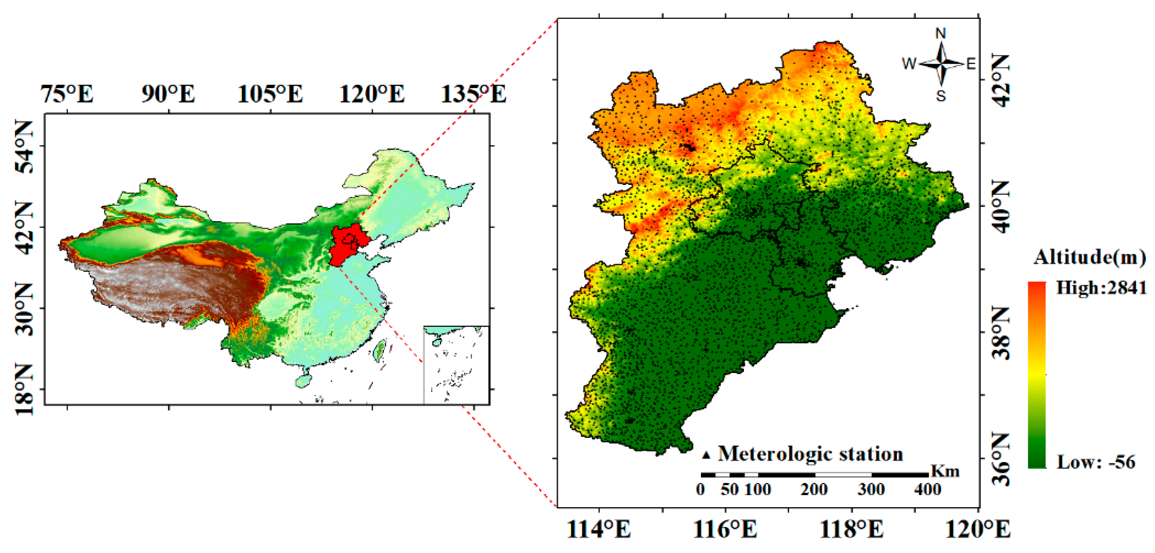
Figure 1. Geographical location and elevation distribution of the study area.
Remotesensing 17 02205 g001
Figure 2. Flowchart of this study.
Remotesensing 17 02205 g002
Figure 3. Boxplot of the difference between observed and estimated SATLR values.
Remotesensing 17 02205 g003
Figure 4. Spatial distribution of mean SATLR for the year.
Remotesensing 17 02205 g004
Figure 5. Moments when the annual mean SATLR reaches its steepest value (a) and shallowest value (b).
Remotesensing 17 02205 g005
Figure 6. Spatial distribution of annual difference in SATLR.
Remotesensing 17 02205 g006
Figure 7. Annual average hourly SATLR time variation curve at different altitude levels.
Remotesensing 17 02205 g007
Figure 8. Seasonal mean SATLR distribution (ad) represent spring–winter, respectively).
Remotesensing 17 02205 g008
Figure 9. Seasons in which monthly mean SATLR reached steepest (a) and shallowest (b).
Remotesensing 17 02205 g009
Figure 10. Moments when the average SATLR reached steepest (ad) and shallowest (eh) values in each season.
Remotesensing 17 02205 g010
Figure 11. Seasonal mean hourly SATLR curve at different altitudes (ad) represent spring–winter, respectively).
Remotesensing 17 02205 g011
Table 1. Accuracy statistics of remote sensing estimates of SATLR for different months.
TimingR2RMSE (°C)MAE (°C)N
January0.8241.71.31188
February0.7941.81.41272
March0.8191.81.41272
April0.8261.91.41271
May0.8291.81.31271
June0.8351.71.31272
July0.8361.41.11318
August0.8341.41.01328
September0.7552.11.51340
October0.822.01.51341
November0.8021.71.31332
December0.8231.91.51333
Full year0.821.81.315,538
Disclaimer/Publisher’s Note: The statements, opinions and data contained in all publications are solely those of the individual author(s) and contributor(s) and not of MDPI and/or the editor(s). MDPI and/or the editor(s) disclaim responsibility for any injury to people or property resulting from any ideas, methods, instructions or products referred to in the content.