MSDCA: A Multi-Scale Dual-Branch Network with Enhanced Cross-Attention for Hyperspectral Image Classification

Abstract

The high dimensionality of hyperspectral data, coupled with limited labeled samples and complex scene structures, makes spatial–spectral feature learning particularly challenging. To address these limitations, we propose a dual-branch deep learning framework named MSDCA, which performs spatial–spectral joint modeling under limited supervision. First, a multiscale 3D spatial–spectral feature extraction module (3D-SSF) employs parallel 3D convolutional branches with diverse kernel sizes and dilation rates, enabling hierarchical modeling of spatial–spectral representations from large-scale patches and effectively capturing both fine-grained textures and global context. Second, a multi-branch directional feature module (MBDFM) enhances the network’s sensitivity to directional patterns and long-range spatial relationships. It achieves this by applying axis-aware depthwise separable convolutions along both horizontal and vertical axes, thereby significantly improving the representation of spatial features. Finally, the enhanced cross-attention Transformer encoder (ECATE) integrates a dual-branch fusion strategy, where a cross-attention stream learns semantic dependencies across multi-scale tokens, and a residual path ensures the preservation of structural integrity. The fused features are further refined through lightweight channel and spatial attention modules. This adaptive alignment process enhances the discriminative power of heterogeneous spatial–spectral features. The experimental results on three widely used benchmark datasets demonstrate that the proposed method consistently outperforms state-of-the-art approaches in terms of classification accuracy and robustness. Notably, the framework is particularly effective for small-sample classes and complex boundary regions, while maintaining high computational efficiency.

1. Introduction

Hyperspectral images classification remains a key research area within the broader field of hyperspectral data analysis, consistently attracting considerable attention from scholars and researchers [1]. This domain focuses on the systematic extraction and interpretation of the rich spectral information embedded in hyperspectral images. By leveraging the distinct spectral signatures of various objects across numerous spectral bands, it facilitates highly accurate pixel-wise classifications [2]. The precision achieved in hyperspectral classification plays a crucial role, not only in advancing the capabilities of hyperspectral remote sensing but also in providing valuable contributions to numerous application areas, including precision agriculture [3], medical imaging [4], mineral exploration [5], food safety monitoring [6], and military surveillance [7]. As highlighted in [8], artificial intelligence-based methods for remote sensing data analysis still face considerable obstacles, including inconsistent sample distributions, high inter-class similarity, and complex contextual dependencies. However, the high dimensionality of HSI data, coupled with limited labeled samples and complex scene structures, poses significant challenges to accurate classification. These factors often hinder the performance of conventional methods, especially in scenarios with spatial heterogeneity or label scarcity.

Early hyperspectral image classification methods predominantly relied on spectral similarity measures, such as the Bhattacharyya distance [9], spectral angle matching (SAM) [10], and the k-Nearest neighbor algorithm (k-NN) [11]. Although these approaches are conceptually simple and easy to interpret, they often suffer from classification errors due to issues like “homoscedasticity” and “heteroscedasticity”. The adoption of machine learning techniques presents a significant step forward in improving classification performance. For instance, techniques for reducing data dimensionality, such as principal component analysis (PCA) [12] and linear discriminant analysis (LDA) [13], have shown higly effective in simplifying the high-dimensional nature of hyperspectral imagery. Currently, classification algorithms such as support vector machines (SVM) [14] and random forests (RF) [15] have been widely adopted to improve the stability and reliability of classification results. While dimensionality reduction and SVM-based techniques have been widely used, their limited ability to model high-order structural information restricts performance. In this regard, nonlocal low-rank tensor modeling has emerged as a promising direction [16], providing enhanced representation power through structured feature decomposition and nonlocal context encoding. These insights underscore the need for models that not only leverage spatial–spectral fusion, but also integrate multi-scale abstraction and inter-feature relational modeling.

To better capture the spatial and spectral information in hyperspectral images, recent research has increasingly adopted deep learning approaches for classification tasks. Although neural networks have existed since the mid-20th century, the surge in computational capabilities and data availability in the early 2000s significantly propelled the progress of deep models. The emergence of deep belief networks (DBNs) [17] in 2006 addressed training difficulties in deep structures, and the success of AlexNet in the 2012 ImageNet challenge marked a turning point for deep learning in visual recognition. In the context of hyperspectral image analysis, deep models have gained prominence for their ability to autonomously and hierarchically extract representative features. For example, Yang et al. introduced a semi-supervised adversarial autoencoder, which leveraged stacked autoencoders [18] to learn more abstract spectral representations, thus enhancing classification accuracy. Building on the proven effectiveness of convolutional neural networks (CNNs) in visual data processing, Hu et al. developed a one-dimensional CNN (1D-CNN) [19] specifically designed for hyperspectral image analysis. This model captures spectral characteristics by passing the input data through a sequence of layers, including convolution, pooling, dense connections, and final classification layers. This development had a profound influence on subsequent CNN-based classification techniques. Zhao et al. later presented a two-dimensional CNN (2D-CNN) [20], which extracted spatial features by reducing the spectral dimensions. However, both of these methods focused primarily on extracting features in a single dimension. Recognizing the inherently three-dimensional structure of hyperspectral imagery, scholars such as Chen [21] and Li [22] pioneered network architectures based on 3D convolutional neural networks (3D-CNNs), allowing the simultaneous and effective extraction of spatial and spectral information. To further improve the classification accuracy, Zhang et al. proposed a hybrid approach that combined 1D-CNN to extract spectral information with 2D-CNN to capture spatial–spectral features. The outputs of these two streams were fused using various strategies, including direct addition, feature concatenation, and their weighted counterparts [23]. Roy et al. subsequently improved this framework by merging the strengths of 2D-CNN and 3D-CNN into a hierarchical architecture [24], which reduced computational complexity while simultaneously increasing classification accuracy by enabling more comprehensive spatial–spectral feature extraction.

In addition to exploring diverse CNN-based architectures for hyperspectral image classification, recent studies have increasingly introduced integrated methods that combine convolutional networks with traditional machine learning techniques and advanced computational strategies. For example, Cao et al. enhanced classification accuracy by combining CNN with Markov random fields for spatial smoothing [25]. Liang et al. extracted compact subspace features from CNN high-level outputs using sparse representation methods to improve spatial–spectral characterization [26]. Zhong et al. proposed the spatial–spectral residual network [27], which employed residual modules in both spectral and spatial branches to enhance feature extraction. This architecture improved the network’s ability to capture complex patterns, leading to more reliable classification outcomes. Attention mechanisms also emerged as a key component in CNN-based hyperspectral models, helping to address the unique spatial–spectral structure of hyperspectral data. He et al. noted that, unlike RGB images, hyperspectral imagery contained a distinct structure combining 2D spatial and spectral dimensions. To address this, they proposed the M3D-CNN [28], a multi-scale 3D convolutional model that jointly learned spatial and spectral features. Building on this direction, Hang et al. proposed a dual-branch attention-integrated CNN [29], which separated spectral and spatial processing to enhance the feature distinctiveness. Wang et al. introduced Cubic-CNN [30], an end-to-end model that incorporated dimensionality reduction while preserving both global and local characteristics. To avoid the limitations of sequential processing, Hang et al. further developed a multi-attention dual-branch architecture [31], enabling efficient parallel learning of spectral and spatial information. Ben Hamida et al. expanded this paradigm by proposing the 3D-DLA [32], which used 3D convolutions for simultaneous spatial–spectral modeling. Beyond CNN-based models, recent research also explored novel architectures such as generative adversarial networks (GANs) [33], capsule networks [34], and graph convolutional networks (GCNs) [35], aiming to overcome the limitations of traditional approaches. These models provided promising alternatives for enhancing classification performance in complex hyperspectral scenes.

While convolutional neural networks (CNNs) had traditionally served as a foundational tool for hyperspectral image analysis, the emergence of transformer-based models [36] introduced novel perspectives and opportunities for advancement in this domain. Originally proposed by Vaswani et al., the transformer architecture was subsequently adapted for a range of computer vision applications. With developments such as the vision transformer (ViT) [37], transformers gained substantial traction in tasks including image classification, object recognition, and semantic understanding. Unlike CNNs, which were constrained by fixed receptive fields, transformer models used self-attention to capture relationships between globally distributed features across an image. This advantage positioned transformers as a powerful alternative to traditional CNN-based approaches, offering improved classification accuracy in hyperspectral imagery.

Even though modeling joint spatial–spectral dependencies in hyperspectral images remains a persistent challenge, recent advances in Transformer-based architectures have introduced promising solutions. He et al. [38] proposed the spatial–spectral transformer, which incorporated dense connectivity to enhance inter-band correlations and improve classification accuracies. Qing et al. [39] developed a transformer-based network using continuous spectral attention for fine-grained spectral dependency learning. Hong et al. [40] introduced SpectralFormer, which employed grouped spectral embedding (GSE) for localized spectral feature extraction and cross-layer adaptive fusion (CAF) for dynamic inter-layer information exchange. To improve semantic representation, Sun et al. [41] proposed SSFTT, which transformed low-level features into semantic tokens and integrated CNNs with transformers for improved spatial–spectral representation. Further innovations included SPRLT-Net by Xue et al. [42], which used recursive local attention to capture fine-grained spatial relationships, and GPE by Mei et al. [43], which directed attention to localized spatial–spectral regions. Fang et al. [44] presented MAR-LT, a lightweight attention-enhanced convolutional framework, while Roy et al. [45] introduced MorphFormer, which combined morphological operations with attention modules to improve geometric feature extraction. These developments collectively highlighted the increasing potential of transformer-based models to advance hyperspectral image classification.

Current HSI classification methods have demonstrated promising performance in capturing spatial and spectral features. However, most rely on fixed-size sampling patches, which limits their ability to model multi-scale contextual information, particularly in complex or heterogeneous scenes. Additionally, generating high-quality pixel-level annotations is labor-intensive and costly, resulting in limited labeled data. This scarcity of supervision, coupled with rigid sampling strategies, constrains model adaptability and classification accuracy. To address these issues, we propose a dual-branch deep learning framework for low-supervision hyperspectral classification. The model integrates multi-scale 3D spatial–spectral convolutions and directional 2D feature encoding to capture both global context and fine-grained spatial structures. A cross-attention transformer module is further introduced to enable semantic alignment and adaptive fusion across heterogeneous branches. This design improves feature discrimination, particularly for small-sample categories and boundary-region pixels, while maintaining high classification accuracy under limited supervision. Extensive experiments on benchmark HSI datasets demonstrate the effectiveness and robustness of the proposed method.

The design of the multi-scale dual-branch network with enhanced cross-attention (MSDCA) incorporates the following three major contributions:

• The multi-scale 3d spatial–spectral feature extraction module (3D-SSF) is designed to learn hierarchical spatial–spectral representations under complex scene conditions using three parallel 3D convolutional branches with varying kernel sizes and dilation rates. It enables the extraction of both fine-grained local features and broad contextual information, supporting effective multi-scale abstraction in heterogeneous land-cover areas.
• The multi-branch directional feature module (MBDFM) is developed to capture axis-specific spatial patterns by applying depthwise separable convolutions along multiple orientations. Through parallel branches with horizontal, vertical, and square-shaped kernels, this module enhances directional sensitivity and long-range spatial structure modeling. As a lightweight 2D complement to the 3D branch, MBDFM improves spatial feature precision without increasing computational complexity.
• An enhanced cross-attention transformer encoder (ECATE) is proposed to perform semantic alignment and adaptive fusion across multi-scale features. It employs a dual-path fusion strategy involving cross-attention between branch-specific tokens and residual-based structural preservation. The fused features are further refined by efficient channel attention and spatial attention, enabling more discriminative representation under complex or weakly supervised scenarios.

2. Materials and Methods

In this section, we elaborate on the proposed MSDCA framework, which is composed of a multi-scale dual-branch architecture, directional feature modeling, and transformer-based semantic fusion. Figure 1 presents the architecture of the proposed MSDCA network.

The overall information flow in MSDCA proceeds as follows: First, the input hyperspectral data undergo PCA-based dimensionality reduction and patch extraction at two different spatial scales. These patches are then fed into a dual-branch feature extraction structure, where the larger-patch branch applies the multi-scale 3D spatial–spectral feature module (3D-SSF), and the smaller-patch branch uses a lightweight convolution to preserve fine-grained spatial details. Both outputs are subsequently passed through the multi-branch directional feature module (MBDFM) to capture directional spatial patterns. The resulting features from each branch are then tokenized and input into the enhanced cross-attention transformer encoder (ECATE), where cross-attention is applied to enable deep semantic interaction between the two streams. Finally, the fused tokens are passed through channel and spatial attention modules and projected into classification scores via a fully connected head.

2.1. HSI Data Preprocessing

Hyperspectral images (HSIs) capture rich spectral information across a large number of bands. However, the resulting high-dimensional data present significant processing challenges. To address this, data preprocessing becomes crucial, as it helps extract meaningful features while reducing computational complexity. Among various preprocessing methods, principal component analysis (PCA) is a commonly used and effective technique to reduce the dimensionality of HSIs data. Consider the original hyperspectral images $\mathit{I}\in {\mathbb{R}}^{M\times N\times L}$, where M and N represent the spatial dimensions (height and width), and L is the number of spectral bands. PCA is then applied along the spectral dimension to reduce the number of bands from L to l, resulting in a transformed image ${\mathit{I}}_{\mathrm{PCA}}\in {\mathbb{R}}^{M\times N\times l}$. This dimensionality reduction technique effectively removes redundant spectral information while maintaining full spatial resolution, ensuring that the essential spatial structure of the images remains intact.

In hyperspectral classification, the sample size is often limited. To make the most of the available training data and enhance the model’s generalization capability, patches of varying sizes are used for feature extraction. To acquire information across multiple scales, the model is designed to extract two patches of different dimensions, $L_1^p\in {\mathbb{R}}^{s_1\times s_1\times l}$ and $L_2^p\in {\mathbb{R}}^{s_2\times s_2\times l}$, where $s_1\times s_1$ and $s_2\times s_2$ denote the respective window sizes. The label assigned to each patch corresponds to the label of its central pixel. During patch extraction, a padding operation is applied to the image boundaries to ensure that edge pixels are adequately handled. Once all 3D patches are generated, those with label values of 0 are discarded. The two extracted variables are then combined to construct a dataset, which serves as input to the network. The generated data samples corresponding to each pixel are stored in set A. Following a given sampling rate, the dataset is randomly divided into training and testing subsets. Both sets contain the corresponding ground truth labels. These labels are represented as $Y\in {\mathbb{R}}^{M\times N}$, where Y is the ground truth labels.

2.2. Double-Branch Multi-Level Spatial–Spectral Feature Extraction Module

As illustrated in Figure 1, the model adopts a dual-branch architecture, where each branch is dedicated to extracting features from image patches of different sizes. The branch processing larger patches, represented as $L_1^p$, is designed to capture global features, while the branch handling smaller patches, denoted as $L_2^p$, emphasizes the modeling of local features. This structure allows the network to effectively learn both global context and fine-grained spatial details by leveraging multi-scale input cubes.

In the first branch, corresponding to the larger patch size $s_1\times s_1$, a multi-scale 3D spectral–spatial joint feature extraction module (3D-SSF) is constructed to extract features using convolutional kernels with varying dilation rates. Once the input feature cube is processed through the 3D-SSF module, three parallel convolutional paths are applied. The first path utilizes eight convolution kernels of size $3\times 3\times 3$ with a dilation rate of 2 to capture features within a medium receptive field. The second path employs eight kernels of size $5\times 5\times 5$, also with a dilation rate of 2, to extract information from a broader spatial context. To obtain global receptive field features, the third path applies eight convolution kernels of size $7\times 7\times 7$. The outputs from these three paths are then fused with their corresponding inputs through element-wise addition, resulting in the final multi-scale 3D feature representation denoted as $L_1^{3\mathrm{D}}$. DConv indicates the use of dilated convolution.

$$\begin{array}{c}\hfill {\mathit{L}}_1^{3\mathrm{D}}=\mathrm{Dilated}{\mathrm{Conv}3\mathrm{D}}_{(3\times 3\times 3)}\left(L_1^p\right)\oplus \mathrm{Dilated}{\mathrm{Conv}3\mathrm{D}}_{(5\times 5\times 5)}\left(L_1^p\right)\\ \hfill \oplus {3\mathrm{DConv}}_{(7\times 7\times 7)}\left(L_1^p\right)\oplus L_1^{3D}\end{array}$$

(1)

In the second branch, which corresponds to the smaller patch size $s_2\times s_2$, a 3D convolutional kernel of size $1\times 3\times 3$ is employed. In this configuration, the kernel maintains a fixed size of 1 along the spectral axis, while a size of 3 is used in the spatial dimensions. This design allows the receptive field to expand solely in the spatial domain, preserving the spectral dimension without alteration. As a result, local spectral features are maintained while spatial context is effectively captured.

$$\begin{array}{c}\hfill {\mathit{L}}_2^{3\mathrm{D}}={3\mathrm{DConv}}_{(1\times 3\times 3)}\left(L_2^p\right)\end{array}$$

(2)

After completing 3D feature extraction, a multi-branch directional feature module (MBDFM) is introduced to further enhance spatial feature representation, capture spatial dependencies across multiple scales, and reduce computational cost. This module adopts a multi-branch parallel structure and leverages depthwise separable convolutions (DWConv) to extract spatial features at different scales. Residual connections are also incorporated to improve the expressiveness of the features and maintain the stability of the gradient flow. The MBDFM module consists of three parallel branches, each tailored to capture features at a specific scale. The first branch applies a $3\times 3$ DWConv to extract local textures and short-range spatial dependencies. The second branch uses a $1\times 11$ DWConv to model long-range dependencies along the horizontal direction. Moreover, the third branch utilizes a $11\times 1$ DWConv to capture long-range dependencies along the vertical direction. The outputs from the three branches are concatenated to form a unified multi-scale joint feature representation. To further improve feature representation, residual connections are applied to the fused features, leading to the final output representation:

$$\begin{array}{cc}\hfill {\mathit{F}}_1=& \mathrm{Concat}\left({\mathrm{DWConv}}_{(3\times 3)}\left(L_1^{3D}\right),{\mathrm{DWConv}}_{(1\times 11)}\left(L_1^{3D}\right),{\mathrm{DWConv}}_{(11\times 1)}\left(L_1^{3D}\right)\right)\oplus L_1^{3D}\hfill \end{array}$$

(3)

$$\begin{array}{cc}\hfill {\mathit{F}}_2=& \mathrm{Concat}\left({\mathrm{DWConv}}_{(3\times 3)}\left(L_2^{3D}\right),{\mathrm{DWConv}}_{(1\times 11)}\left(L_2^{3D}\right),{\mathrm{DWConv}}_{(11\times 1)}\left(L_2^{3D}\right)\right)\oplus L_2^{3D}\hfill \end{array}$$

(4)

2.3. Enhanced Cross-Multi-Attention Transformer Encoder Module

Once the multi-scale 2D feature information is extracted from the dual-branch multi-level spatial–spectral feature extraction module, a tokenization step is performed to improve compatibility with the transformer framework. The extracted features $F_1$ and $F_2$ are first flattened into sequences. These flattened features are then projected through linear transformations to obtain token representations. Subsequently, token representations are derived via linear transformations, followed by feature weighting using the softmax function.

Then, the learnable classification token $T_{\mathrm{cls}}$ is added as an additional feature, followed by the positional encoding $P{E}_{pos}$, resulting in the final token sequences:

$$\begin{array}{c}\hfill {\mathit{T}}_1=[T_f^1;T_{\mathrm{cls}}]\oplus P{E}_{pos}{\mathit{T}}_2=[T_f^2;T_{\mathrm{cls}}]\oplus P{E}_{pos}\end{array}$$

(5)

However, these tokens still represent localized features derived from different layers and branches of the network. To enhance interdependence and interaction among these tokens, an enhanced cross-multi-attention feature fusion module is introduced, as illustrated in Figure 2.

Following the notation introduced in the previous module, the extracted tokens $T_1$ and $T_2$ are processed through convolutional layers with different kernel sizes to generate their corresponding attention tensors. For $T_1$, a $3\times 3$ 2D convolution with padding set to 1 is first applied to obtain $Q_{T_1}$. Then, a $5\times 5$ dilated convolution with a padding of 2 is used to produce $K_{T_1}$. Finally, a $3\times 3$ dilated convolution with a dilation rate of 2 is used to obtain $V_{T_1}$. In this case, the convolution kernel is a $3\times 3$ matrix, but the dilation rate of 2 means that the kernel elements are spaced apart by one pixel between them. This increases the receptive field of the convolution operation, allowing the model to capture a wider context in the input without increasing the number of parameters. Similarly, $T_2$ is initially passed through a $3\times 3$ convolution with padding of 1 to generate $Q_{T_2}$. This is followed by a $3\times 3$ convolution with a dilation factor of 2 is applied to obtain $K_{T_2}$. Lastly, a $5\times 5$ convolution is performed to obtain $V_{T_2}$. Through this process, $T_1$ is enriched by integrating information from $V_{T_2}$, and $T_2$ is refined using $V_{T_1}$, thereby enabling complementary fusion of global semantic information.

Subsequently, deep interactions between the two branches are facilitated using the cross-attention mechanism, resulting in the generation of cross-features $A_{T_1}$ and $A_{T_2}$.

$$\begin{array}{c}\hfill {\mathit{A}}_{T_1}=\mathrm{Softmax}\left({\displaystyle \frac{Q_{T_1}{K}_{T_1}^{\top }}{\sqrt{d_k}}}\right)V_{T_2}\end{array}$$

(6)

$$\begin{array}{c}\hfill {\mathit{A}}_{T_2}=\mathrm{Softmax}\left({\displaystyle \frac{Q_{T_2}{K}_{T_2}^{\top }}{\sqrt{d_k}}}\right)V_{T_1}\end{array}$$

(7)

To enable effective interaction between ${\mathit{A}}_{T_1}$ and ${\mathit{A}}_{T_2}$, we concatenate and normalize them before feeding into an MLP to derive ${\mathit{A}}_{\mathrm{cross}}$.

$$\begin{array}{c}\hfill {\mathit{A}}_{\mathrm{cross}}=MLP\left(LN(A_{T_1}\oplus A_{T_2})\right)\end{array}$$

(8)

To capture local interactions between $T_1$ and $T_2$, we employ a 2D convolution on their concatenated representation, resulting in the fused output ${\mathit{A}}_{\mathrm{fused}}$.

$$\begin{array}{c}\hfill {\mathit{A}}_{\mathrm{fused}}=2DConv(T_1\oplus T_2)\end{array}$$

(9)

During the fusion stage, we apply a grouped $1\times 1$ convolution to both ${\mathit{A}}_{\mathrm{cross}}$ and ${\mathit{A}}_{\mathrm{fused}}$, followed by BatchNorm and ReLU, to perform a lightweight channel-wise transformation. This operation reduces computational complexity while maintaining inter-channel dependencies. To further enhance the quality of the fused features, the module integrates both the efficient channel attention (ECA) and spatial attention (SA) mechanisms, as depicted in Figure 3. Specifically, ECA computes channel-wise weights by applying adaptive average pooling followed by a one-dimensional convolution, enabling dynamic reweighting of channel responses. In parallel, SA emphasizes spatially informative regions to complement the channel-wise enhancement. The final fused feature, denoted as $\widehat{T}$, is subsequently used as the input to the classifier. The complete process can be formulated as

$$\begin{array}{c}\hfill {\mathit{A}}_{\mathrm{ECA}}=\left(\sigma \left(2Dconv(2DGroupConv\left(A_{cross}\right)\oplus 2DGroupConv\left(A_{fused}\right))\right)\right)\otimes A_{fused}\oplus A_{fused}\end{array}$$

(10)

$$\begin{array}{c}\hfill \widehat{\mathit{T}}=\mathrm{SA}\left(\mathrm{ECA}\left({\mathit{A}}_{\mathrm{ECA}}\right)\right)\end{array}$$

(11)

where $\sigma$ is the sigmoid activation function and $2DGroupConv(·)$ is a 2D grouped convolution that processes grouped channels separately to improve efficiency.

The complete procedure of the proposed MSDCA is outlined in Algorithm 1.

Algorithm 1 MSDCA Model.

Input: The input HSI data $I\in {\mathbb{R}}^{M\times N\times L}$, with truth labels $Y\in {\mathbb{R}}^{a\times b}$. PCA parameter $l=30$. Extract two sets of feature cubes: $L_1^p\in {\mathbb{R}}^{s_1\times s_1\times l}$ and $L_2^p\in {\mathbb{R}}^{s_2\times s_2\times l}$, where $s_1>s_2$. The training dataset is divided in a ratio of 1:99. Output: Predicted labels for the test dataset.  1: The batch size is 64, and learning rate is $5\times {10}^{-4}$. The training epochs, $\epsilon =500$.  2: The dataset after PCA dimensionality reduction is represented as $I_{\mathrm{PCA}}\in {\mathbb{R}}^{M\times N\times l}$.  3: Extract the data $L_1^p$ and $L_2^p$, and place them into a set A. Then, divide the set A into training and test subsets using a sampling ratio of 1:99.  4: for $i=1$ to $ϵ$ do  5:     The data $L_1^p$ and $L_2^p$ are processed by a dual-branch multi-level spatial spectrum feature extraction module to generate features $F_1$ and $F_2$.  6:     The features $F_1$ and $F_2$ are used to obtain the labeled sequences $T_1$ and $T_2$ through Equation (5).  7:     The tokens $T_1$ and $T_2$ are passed through the ECATE, resulting in the fused spectral–spatial enhanced feature $\widehat{T}$ through Equation (11).  8:     The learnable classification token is passed through a linear layer, and the classification probabilities are computed using the Softmax function.  9: end for   10: The trained model is applied to the test dataset to generate predicted labels.

2.4. Classifier Head

For the HSI classification task, the fully connected classifier head (FCCH) is employed to produce the final classification output. Specifically, a learnable classification token (CLS Token) is extracted from the enhanced cross-multi-attention transformer encoder module, which encapsulates a global representation of the entire input. This token is then passed through the multilayer perceptron (MLP) classification head to generate the final prediction. The MLP head consists of several fully connected (FC) layers. Each of these layers is followed by layer normalization (LN), thus generating a prediction vector $I\in {\mathbb{R}}^{1\times C}$, where C denotes the total number of categories. To interpret these outputs probabilistically, a Softmax function is applied across the vector elements, converting the raw logits into a categorical probability distribution that satisfies the normalization condition ${\sum }_{i=1}^C{p}_i=1$. The class label assigned to each input sample is then determined by identifying the index corresponding to the highest probability in this distribution.

The entire classification process can be formulated as follows:

$$\begin{array}{c}\hfill I=\mathrm{Softmax}\left(\mathrm{FC}\left(\mathrm{LN}\left({\widehat{T}}_{\mathrm{cls}}\right)\right)\right)\end{array}$$

(12)

3. Results

In this section, we evaluate the effectiveness of the proposed methods through extensive experiments conducted on three publicly available datasets. First, we provide an overview of the three datasets used in the study. Then, the experimental setup is detailed, followed by a parametric analysis. Next, we present the classification results along with an evaluation of our method and comparative approaches. Finally, ablation experiments are systematically conducted to examine how each module influences the model’s performance, allowing for a clearer understanding of their individual contributions.

Table 1. Training and testing split for all three datasets.

No.	Houston2013 Dataset			Trento Dataset			Pavia University Dataset
	Class	Training	Testing	Class	Training	Testing	Class	Training	Testing
#1	Healthy Grass	13	1238	Apple Trees	40	3994	Asphalt	66	6565
#2	Stressed Grass	13	1241	Buildings	29	2874	Meadows	186	18,463
#3	Synthetic Grass	7	690	Ground	5	474	Gravel	21	2078
#4	Tree	12	1232	Woods	91	9032	Trees	31	3033
#5	Soil	12	1230	Vineyard	105	10,396	Metal Sheets	13	1332
#6	Water	3	322	Roads	31	3143	Bare soil	50	4979
#7	Residential	13	1255				Bitumen	13	1317
#8	Commercial	12	1232				Bricks	37	3645
#9	Road	13	1239				Shadows	9	938
#10	Highway	12	1215
#11	Railway	12	1223
#12	Parking Lot 1	12	1221
#13	Parking Lot 2	5	464
#14	Tennis Court	4	424
#15	Running Track	7	653
	Total	150	14,879	Total	301	29,913	Total	426	42,350

presents the sample distribution for the training and test sets, detailing the specific data for each category division.

3.1. Data Description

Our proposed model is validated on three publicly available datasets, which are described in the following.

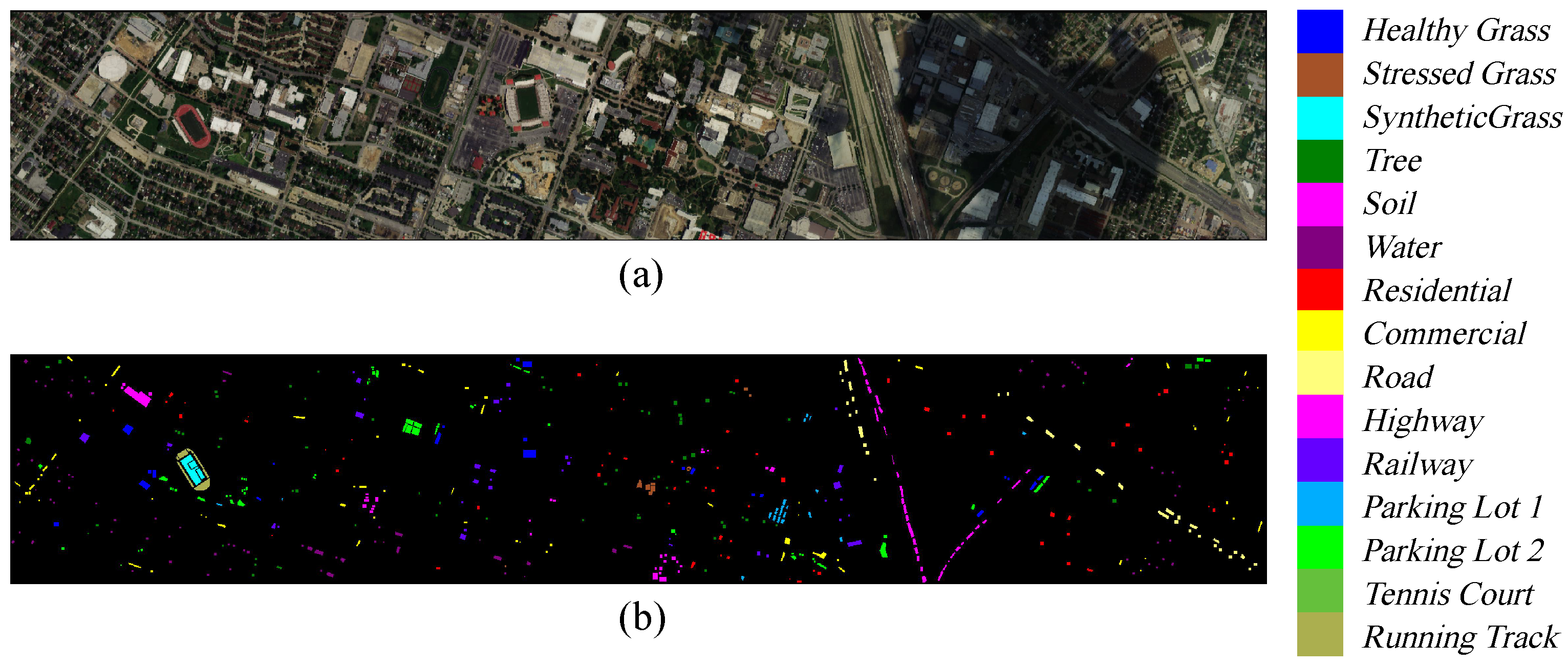
(1) Houston2013 dataset: The Houston 2013 dataset is collaboratively provided by the University of Houston research group and the U.S. National Mapping Center. It comprises 15 land cover classes and includes 144 spectral bands spanning a wavelength range of 0.38∼1.05 μm. The dataset consists of $349\times 1905$ pixels with a spatial resolution of 2.5 m/pixel. Pseudo-color images and ground-truth classification maps are illustrated in Figure 4a,b.

(2) Pavia University: The Pavia University dataset was acquired in 2001 over the University of Pavia in northern Italy using the Reflectance Optical System Imaging Spectrometer (ROSIS) sensor. The original dataset contains 115 spectral bands covering a wavelength range from 0.43 to 0.86 micrometers. The image has spatial dimensions of $610\times 340$ pixels and a spatial resolution of 1.3 m/pixel, and it includes nine land cover categories. To reduce the impact of noise, 12 noisy bands were removed during the experimental process. Pseudo-color images and the corresponding ground truth classification maps are shown in Figure 5a,b.

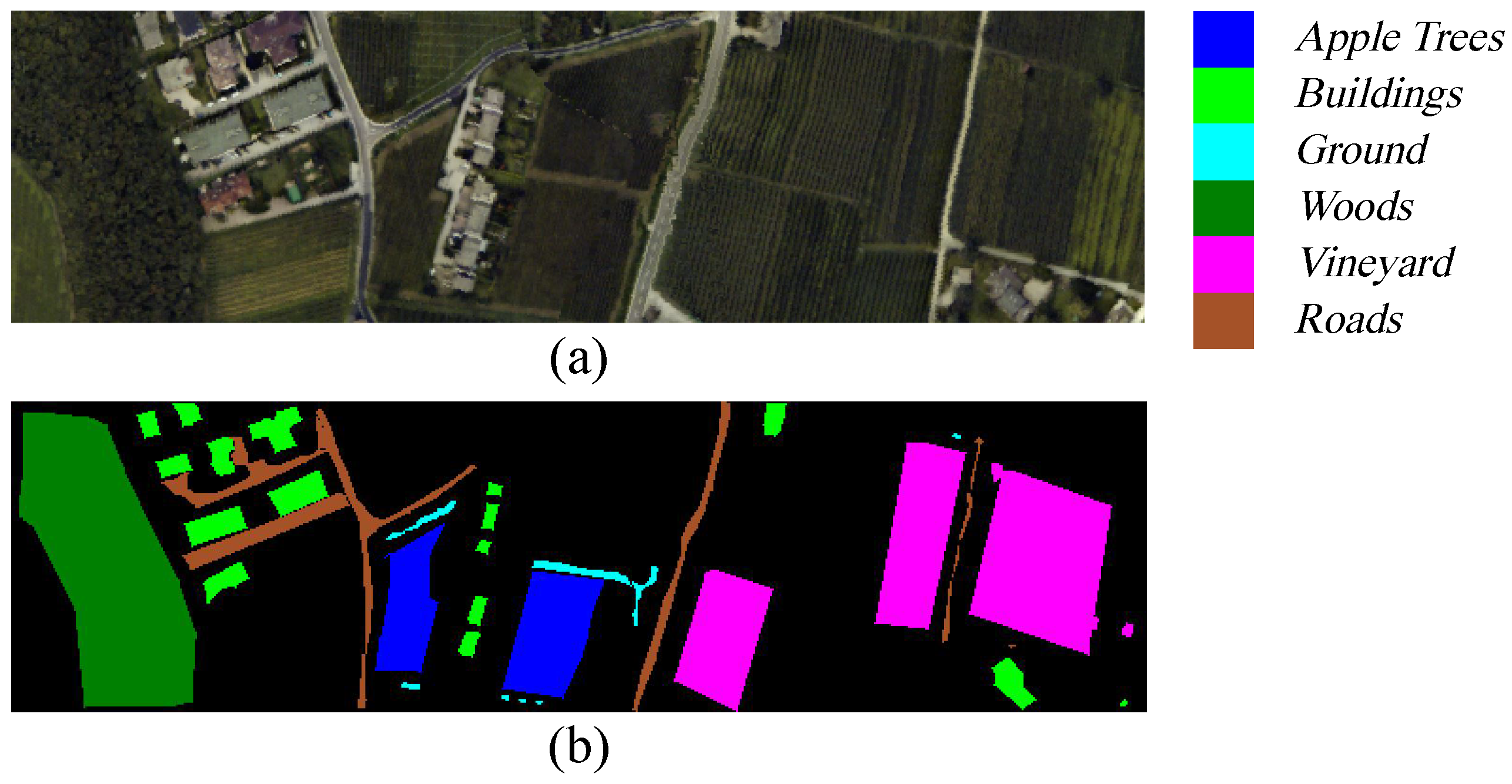
(3) Trento dataset: The Trento dataset was acquired using the AISA Eagle hyperspectral imaging sensor over a rural area located south of Trento, Italy. It consists of 63 spectral bands covering a wavelength range from 0.42∼0.99 μm, with an image size of $600\times 166$ pixels used for classification. The spatial resolution is 1 m/pixel, and the dataset includes six land cover categories. Figure 6a,b display the pseudo-color composite of the hyperspectral data and the corresponding ground truth classification map, respectively.

3.2. Parameter Analysis

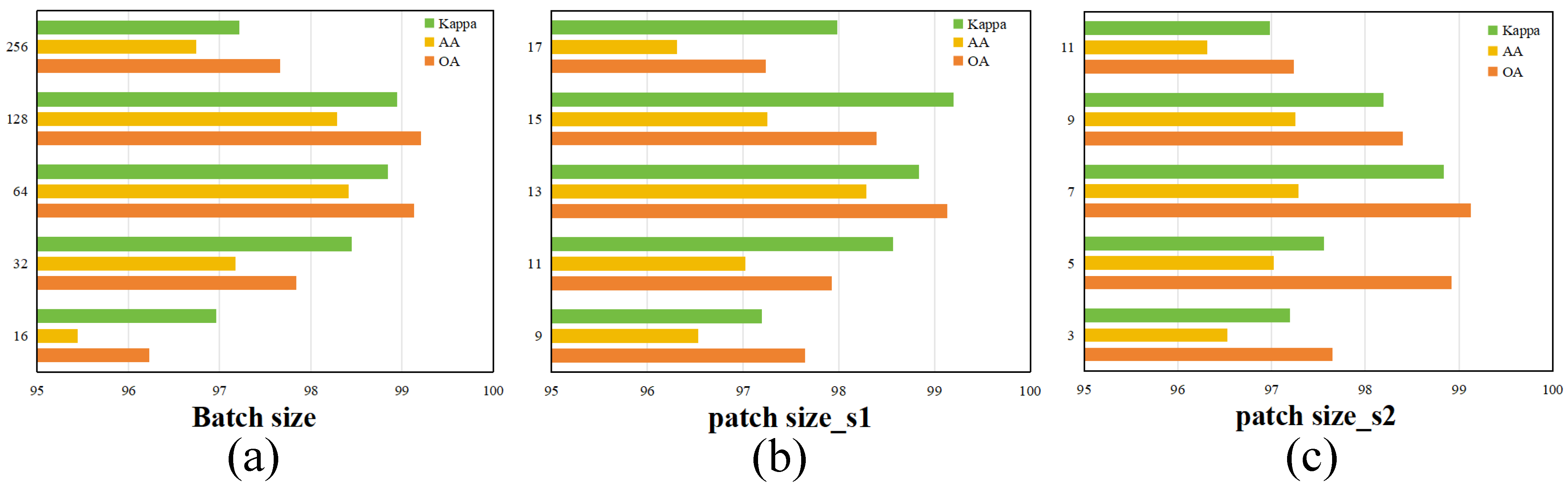
Key hyperparameters of the proposed model, namely, the batch size and the sizes of the first and second cubic patches, were systematically analyzed through experimental evaluation. The results, shown in Figure 7, Figure 8 and Figure 9, offer insight into their optimal configurations.

(1) Batch Size: Batch size plays a vital role in shaping the behavior and performance of deep learning models. It affects not only how efficiently the network is trained and how much memory is utilized but also influences the model’s predictive accuracy and ability to generalize to unknown data. Employing a larger batch size typically speeds up convergence due to more stable gradient estimates but comes at the cost of increased memory usage. Conversely, smaller batch sizes, while less demanding computationally, can introduce higher variance in gradient updates, potentially leading to overfitting or unstable training dynamics. Given these trade-offs, determining the most suitable batch size requires balancing hardware limitations with the needs of the specific learning task. To explore this balance, we conducted a series of experiments using batch sizes selected from the set $16,32,64,128,256$, ensuring that all other hyperparameters remained fixed. The experimental findings revealed that a batch size of 64 yielded the most favorable classification results in the evaluation metrics, indicating its effectiveness under the given model and dataset conditions.

(2) Patch Size: In hyperspectral image (HSI) classification, the size of the input patch plays a critical role in determining the model performance. Larger patches tend to capture more extensive spatial contexts, which can enrich feature representation and support more informed predictions. However, this advantage comes at the cost of increased memory usage and computational complexity. In contrast, smaller patches highlight fine-grained local structures but may fail to preserve essential spatial dependencies among neighboring pixels. To balance these factors, the proposed model adopts a dual-branch architecture that leverages feature representations at multiple spatial scales. Specifically, one branch processes a relatively larger patch to gather broader contextual cues, while the other focuses on a smaller patch to retain local detail. This multiscale strategy makes patch size a key variable that influences classification accuracy.

To identify the most effective patch configurations, we conducted controlled experiments by independently adjusting the patch size for each branch while keeping all other hyperparameters constant. For the first branch, patch sizes were selected from the set $9,11,13,15,17$, and for the second branch, from $3,5,7,9,11$. The evaluation results indicate that the highest classification accuracy is achieved when the first branch uses a patch size of 13 and the second branch operates on a patch size of 7.

3.3. Classification Results and Analysis

To validate the effectiveness of our proposed model, we conduct a series of comparative experiments against several widely baseline methods, including SVM [14], 1D-CNN [19], 3D-CNN [21], M3D-CNN [28], 3D-DLA [32], SSFTT [41], MorphFormer [45], and TNAAC [46]. For each baseline, we adhere to the original implementations by preserving their network configurations and training protocols as documented in their respective publications. 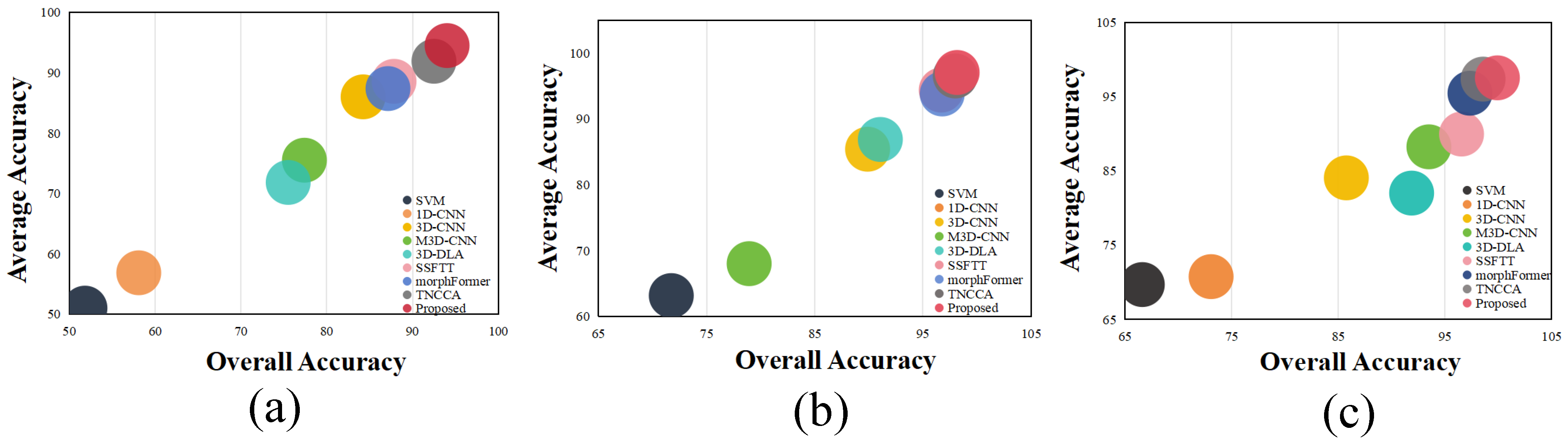Moreover, to ensure a fair comparison, all models are trained and evaluated using the same number of samples, which are randomly selected according to the ratios listed in Table 1. A visual summary of the classification results across multiple datasets is provided in Figure 10, allowing for an intuitive performance comparison. The experimental findings clearly indicate that our MSDCA model achieves superior classification accuracy across the board, outperforming all other approaches in a consistent manner.

(1) Quantitative Results and Analysis: The results of the experiments are presented in

Table 2. Classification performance of various methods on the Houston2013 dataset.

No.	SVM [14]	1D-CNN [19]	3D-CNN [21]	M3D-CNN [28]	3D-DLA [32]	SSFTT [41]	morphFormer [45]	TNCCA [46]	MSDCA
$HealthyGrass$	73.04 ± 10.54	81.42 ± 6.17	91 ± 0.91	91.65 ± 2.17	87.95 ± 5.5	85.79 ± 1.77	96.55 ± 1.79	95.02 ± 2.03	94.04 ± 0.04
$StressedGrass$	43.76 ± 32.43	88.56 ± 2.91	96.28 ± 0.46	88.48 ± 6.02	91.56 ± 3.46	89.86 ± 6.54	96.30 ± 2.01	96.13 ± 1.56	98.47 ± 0.11
$SyntheticGrass$	38.9 ± 46.88	100 ± 0.00	99.74 ± 0.24	98.17 ± 1.56	95.28 ± 1.51	91.36 ± 9.89	98.21 ± 0.72	94.62 ± 1.32	99.86 ± 0.00
$Tree$	13.13 ± 13.09	73.99 ± 18.32	94.71 ± 0.16	84.92 ± 5.59	88.86 ± 2.44	91.01 ± 3.56	93.15 ± 1.63	91.56 ± 2.34	91.79 ± 0.07
$Soil$	78.72 ± 20.41	96.23 ± 3.77	99.98 ± 0.04	97.67 ± 1.56	95.25 ± 3.73	99.75 ± 0.21	91.36 ± 5.63	100 ± 0.00	99.92 ± 0.00
$Water$	22.05 ± 33.46	54.47 ± 16.57	94.7 ± 1.59	52.17 ± 23.97	65.34 ± 16.07	83.23 ± 1.45	79.60 ± 4.32	91.85 ± 3.45	97.35 ± 0.14
$Residential$	11.03 ± 12.42	45.2 ± 17.79	68.49 ± 2.6	57.07 ± 9.75	64.03 ± 4.48	74.32 ± 3.69	77.71 ± 4.59	89.57 ± 3.84	98.25 ± 0.06
$Commercial$	25.1 ± 12.15	23.59 ± 7.01	67.82 ± 3.25	68.62 ± 7.38	57.18 ± 2.97	69.45 ± 2.36	65.26 ± 1.98	82.44 ± 3.53	81.53 ± 0.23
$Road$	7.38 ± 5.72	75.09 ± 11.58	69.73 ± 1.89	50.73 ± 4.13	70.54 ± 5.29	89.21 ± 3.59	88.69 ± 3.99	88.57 ± 3.09	92.78 ± 0.07
$Highway$	11.79 ± 13.79	21.32 ± 19.99	87.28 ± 3.19	85.27 ± 5.52	69.51 ± 5.77	95.02 ± 1.51	89.64 ± 9.25	92.02 ± 2.60	94.45 ± 0.11
$Railway$	10.55 ± 13.45	24.74 ± 9.79	75.47 ± 2.4	75.06 ± 7.53	68.29 ± 7.34	92.46 ± 5.31	88.31 ± 1.03	81.97 ± 5.79	89.76 ± 0.23
$ParkingLot1$	4.67 ± 4.34	35.45 ± 20.73	68.73 ± 2.75	76.77 ± 12.63	80.92 ± 4.18	82.49 ± 4.36	74.56 ± 3.32	89.46 ± 2.31	94.23 ± 0.11
$ParkingLot2$	3.45 ± 3.34	4.96 ± 2.97	71.55 ± 6.4	16.85 ± 6.23	11.38 ± 4.51	84.69 ± 5.40	85.01 ± 3.30	90.89 ± 3.58	89.74 ± 0.45
$TennisCourt$	67.45 ± 2.85	28.63 ± 19.9	99.58 ± 0.48	89.06 ± 12.8	36.6 ± 5.14	99.86 ± 0.14	90.63 ± 4.12	100 ± 0.00	100 ± 0.00
$RunningTrack$	99.17 ± 0.55	99.26 ± 0.27	99.85 ± 0.00	99.97 ± 0.07	94.64 ± 3.53	100 ± 0.00	97.66 ± 0.87	100 ± 0.00	100 ± 0.00
OA (%)	31.82 ± 7.02	58.09 ± 2.59	84.24 ± 0.61	77.4 ± 1.59	75.51 ± 1.07	87.85 ± 1.21	87.14 ± 0.90	92.50 ± 0.80	94.03 ± 0.04
AA (%)	34.01 ± 7.11	56.86 ± 3.35	85.99 ± 0.39	75.5 ± 2.66	71.82 ± 0.72	88.56 ± 0.91	87.36 ± 0.86	91.88 ± 0.75	94.48 ± 0.05
κ × 100	26.75 ± 7.46	54.71 ± 2.76	82.96 ± 0.66	75.52 ± 1.73	73.45 ± 1.16	86.87 ± 1.29	86.45 ± 0.91	90.97 ± 0.58	93.54 ± 0.05

Note: Italic values denote the names of land-covers. Bold values indicate the optimal results.

,

Table 3. Classification results of various methods on the Pavia University dataset.

No.	SVM [14]	1D-CNN [19]	3D-CNN [21]	M3D-CNN [28]	3D-DLA [32]	SSFTT [41]	morphFormer [45]	TNCCA [46]	MSDCA
$Asphalt$	94.1 ± 0.1	93.05 ± 0.59	93.08 ± 1.06	85.75 ± 7.33	93.59 ± 0.99	97.31 ± 0.52	96.51 ± 0.48	97.74 ± 1.31	97.98 ± 0.42
$Meadows$	93.36 ± 0.48	96.78 ± 0.39	96.86 ± 0.81	92.9 ± 2.87	97.64 ± 0.53	98.46 ± 0.21	99.64 ± 0.10	99.98 ± 0.01	99.95 ± 0.03
$Gravel$	0 ± 0	0 ± 0	54.58 ± 3.66	41.45 ± 7.27	75.25 ± 2.95	82.55 ± 2.10	83.21 ± 1.45	86.37 ± 5.12	88.36 ± 0.51
$Trees$	33.39 ± 1.7	23.86 ± 7.02	94.45 ± 0.65	79.82 ± 10.63	83.9 ± 3.45	94.97 ± 1.89	96.09 ± 2.11	97.46 ± 0.39	97.32 ± 1.41
$MetalSheets$	33.39 ± 1.7	23.86 ± 7.02	94.45 ± 0.65	79.82 ± 10.63	83.9 ± 3.45	94.97 ± 1.89	96.09 ± 2.11	97.46 ± 0.39	97.32 ± 1.41
$Baresoil$	17.94 ± 1.9	7.51 ± 1	76.75 ± 3.01	53.87 ± 10.34	80.11 ± 2.16	99.45 ± 0.32	99.46 ± 0.18	99.69 ± 0.11	98.72 ± 1.91
$Bitumen$	0 ± 0	0 ± 0	70.07 ± 4.42	48.65 ± 16.72	79.26 ± 3.27	99.46 ± 0.28	80.01 ± 5.29	99.02 ± 0.80	97.42 ± 1.38
$Bricks$	89.48 ± 0.66	90.86 ± 1.36	84.43 ± 2.41	63.05 ± 20.39	85.33 ± 1.01	95.71 ± 1.68	94.86 ± 1.18	95.21 ± 1.20	94.1 ± 4.31
$Shadows$	50.98 ± 9.84	63.82 ± 10.74	99.59 ± 0.42	52.93 ± 25.23	88.06 ± 5.61	82.47 ± 6.54	93.41 ± 1.60	98.11 ± 0.04	99.81 ± 0.1
OA (%)	71.73 ± 0.27	69.74 ± 0.75	89.88 ± 0.1	78.93 ± 5.94	91.06 ± 0.65	96.69 ± 0.25	96.78 ± 0.47	97.99 ± 0.13	98.16 ± 0.72
AA (%)	53.15 ± 1.3	46.34 ± 1.83	85.38 ± 0.71	68 ± 9.11	86.86 ± 0.81	94.36 ± 0.49	93.77 ± 0.92	96.50 ± 0.80	97.03 ± 1.17
$\kappa$ × 100	60.54 ± 0.48	56.94 ± 1.17	86.49 ± 0.13	71.47 ± 8.14	88.04 ± 0.88	95.88 ± 0.60	96.23 ± 0.41	98.10 ± 0.45	97.64 ± 1.04

Note: Italic values denote the names of land-covers. Bold values indicate the optimal results.

and

Table 4. Classification results of different methods on the Trento dataset.

No.	SVM [14]	1D-CNN [19]	3D-CNN [21]	M3D-CNN [28]	3D-DLA [32]	SSFTT [41]	morphFormer [45]	TNCCA [46]	MSDCA
$AppleTrees$	17.89 ± 4.33	21.95 ± 5.05	97.97 ± 1.09	95.46 ± 1.20	86.32 ± 0.57	99.45 ± 0.17	99.42 ± 0.41	99.60 ± 0.31	99.76 ± 0.08
$Buildings$	46.05 ± 13.28	73.78 ± 11.42	58.02 ± 2.22	78.49 ± 2.46	81.16 ± 0.59	97.21 ± 0.52	92.77 ± 1.30	98.11 ± 0.41	97.24 ± 1.48
$Ground$	51.09 ± 15.33	85.88 ± 5.69	91.98 ± 1.73	68.49 ± 15.04	70.74 ± 1.21	54.26 ± 1.97	91.37 ± 4.17	97.26 ± 1.09	96.25 ± 2.18
$Woods$	70.08 ± 3.74	55.29 ± 7.46	99.95 ± 0.07	97.84 ± 0.23	96.96 ± 1.24	100 ± 0.00	99.95 ± 0.02	100 ± 0.00	100 ± 0.00
$Vineyard$	75.81 ± 7.13	36.32 ± 3.99	78.44 ± 3.89	97.82 ± 0.45	99.40 ± 0.49	99.92 ± 0.08	99.85 ± 0.11	100 ± 0.00	100 ± 0.00
$Roads$	64.21 ± 21.32	69.33 ± 12.08	77.96 ± 4.58	85.04 ± 0.55	80.25 ± 0.42	89.46 ± 2.70	92.44 ± 1.05	93.21 ± 1.63	94.96 ± 0.32
OA (%)	66.62 ± 2.36	73.07 ± 1.56	85.75 ± 1.09	93.49 ± 0.60	91.87 ± 0.88	97.55 ± 0.31	98.34 ± 0.04	98.57 ± 0.24	98.91 ± 0.2
AA (%)	49.69 ± 4.29	56.76 ± 1.05	84.06 ± 0.74	88.24 ± 3.64	82.01 ± 0.40	89.96 ± 0.57	95.46 ± 0.85	97.36 ± 0.55	97.53 ± 0.64
$\kappa$ × 100	56.59 ± 3.32	59.5 ± 1.7	81.28 ± 1.35	92.91 ± 0.55	90.65 ± 0.63	97.24 ± 0.21	97.84 ± 0.21	98.14 ± 0.20	98.54 ± 0.27

Note: Italic values denote the names of land-covers. Bold values indicate the optimal results.

, where the best-performing scores are distinctly marked for clarity. These evaluations were conducted on three widely used hyperspectral image datasets: Houston2013, Pavia University, and Trento. Performance was assessed using several standard classification indicators, including overall accuracy (OA), average accuracy (AA), the Kappa coefficient, and classification accuracy for each individual category. Taking the Houston2013 dataset as a representative example, MSDCA achieves the highest accuracy in categories such as “StressedGrass”, “Water”, “Residential”, “Road”, “ParkingLot1”, “TennisCourt”, and “RunningTrack”. Even in classes such as “HealthyGrass”, “SyntheticGrass”, and “Soil”, where MSDCA does not produce the highest accuracy, it still achieves highly competitive results. In contrast, traditional approaches such as SVM and 1D-CNN demonstrate inferior performance in specific categories. This clearly highlights that, especially in limited-sample scenarios, MSDCA effectively captures multiscale features and fully leverages the spatial–spectral characteristics of HSI data, thus significantly boosting classification performance. Moreover, our method achieves superior results in the Houston2013 dataset, mainly due to the discrete and localized distribution of sample points within this dataset. In contrast, the other two datasets typically contain broader regions of homogeneous classes. Consequently, our model exhibits a semantic modeling advantage in the Houston2013 dataset, thus providing improved classification accuracy.

Our method achieves the best precision in classifying categories including “Asphalt”, “Tree”, “MetalSheets”, and “Shadows” in the Pavia University dataset, as well as “AppleTrees”, “Woods”, “Vineyard”, and “Roads” in the Trento dataset. Conversely, categories such as “Meadows”, “Bitumen”, and “Bricks” in the Pavia University dataset, and “Building” and “Ground” in the Trento dataset, demonstrate moderate classification performance. As indicated in Table 3, the TNCCA model achieves similar or slightly superior accuracy compared to MSDCA for certain individual classes. This is largely attributed to the relatively limited number of samples within these specific categories. Moreover, due to the percentage-based random sampling approach employed, these categories inherently possess fewer training instances, resulting in notable class imbalance.

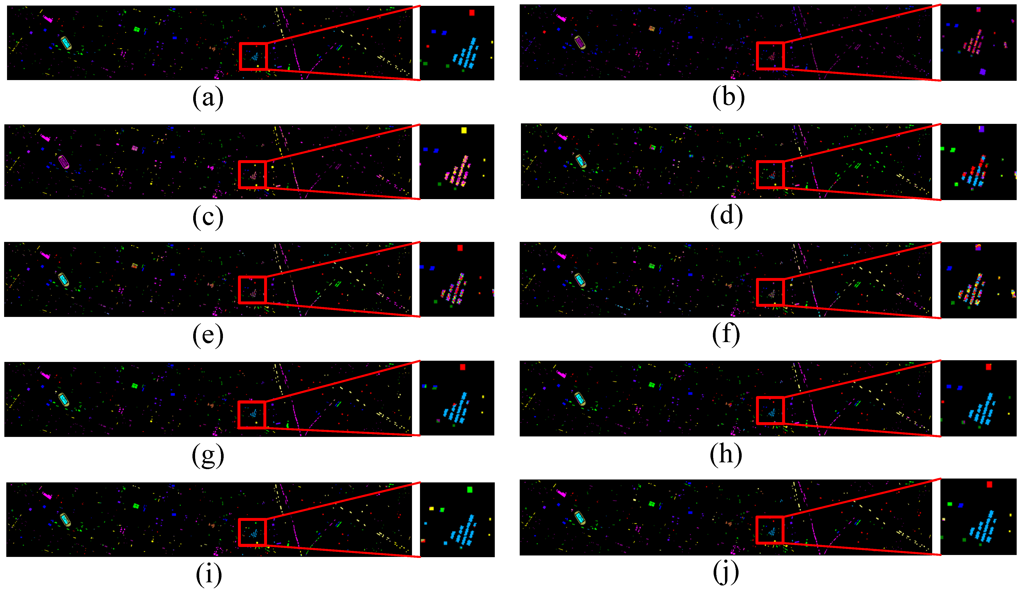
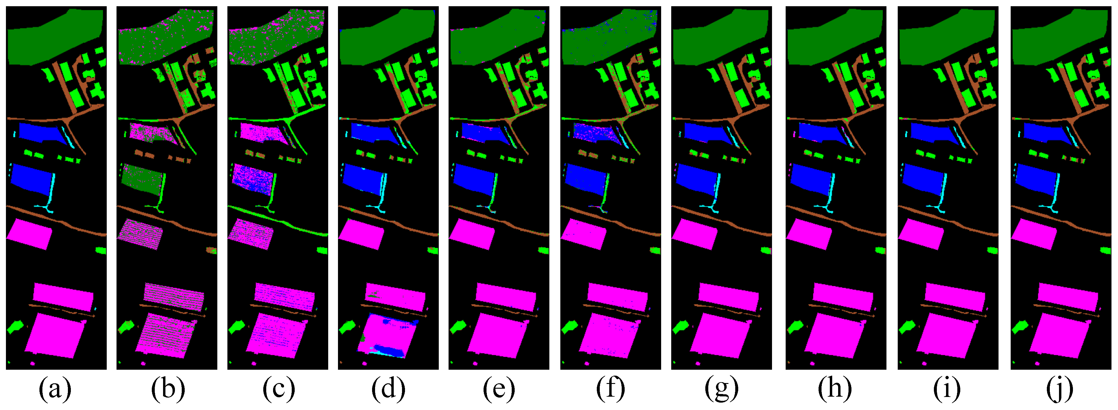
(2) Visual Evaluation and Analysis: Figure 11, Figure 12 and Figure 13 provide visual representations of the classification results through corresponding classification maps. These visualizations, when compared with the spatial distribution of noise observed in the original hyperspectral images, offer intuitive insight into the performance differences among competing methods. From these comparisons, it becomes evident that our proposed approach yields more precise and coherent classification outcomes, effectively reducing misclassification in complex or noisy regions, and consistently surpassing the performance of other evaluated models.

Visually, the classification maps generated by the MSDCA model display clear spatial delineation and minimal background interference. In contrast, the outputs produced by alternative methods generally suffer from less distinct boundaries and a higher presence of classification noise. Taking the Houston2013 dataset as a representative case, the map predicted by our model exhibits strong visual agreement with the ground truth annotations. However, baseline models such as SVM, 1D-CNN, 3D-CNN, M3D-CNN, and 3D-DLA tend to generate more frequent misclassifications and noise-induced artifacts, particularly in complex regions. A closer examination of the zoomed-in sections reveals that MSDCA achieves superior performance in accurately identifying specific land cover types, such as “ParkingLot1”, “StressedGrass”, and “Road”. These improvements are evident in the clarity and consistency of the classified regions. The improved performance of MSDCA on the Houston2013 dataset stems from both the structural complexity of the data and the architectural design of our model. The presence of spectrally similar yet spatially fragmented classes, such as “ParkingLot1” and “StressedGrass”, challenges traditional models. MSDCA addresses this through its dual-branch structure, which combines local spatial–spectral detail extraction with global contextual modeling. Furthermore, directional encoding via MBDFM and semantic fusion through ECATE enhance the model’s ability to handle intricate spatial layouts, resulting in clearer boundaries and reduced misclassification, as illustrated in Figure 12 and Table 2. Likewise, in the Pavia University dataset, the model demonstrates its ability to distinguish the “Bare Soil” category with high precision. While competing approaches often misclassify this region, which introduces erroneous green patches, our method substantially reduces both classification errors and visual noise. These observations underscore the enhanced robustness and spatial awareness of the MSDCA framework across diverse scenarios.

Ultimately, the experimental results confirm that our model consistently outperforms alternative techniques, showcasing its robustness and efficiency in feature representation, even in scenarios with limited samples.

3.4. Analysis of Inference Speed

To assess the inference performance of the MSDCA framework, we recorded both training and evaluation durations across benchmark datasets. The results indicate that the proposed model exhibits notable computational efficiency, managing to complete 500 training epochs within a compact overall runtime. It is worth noting that model evaluation was conducted following each training epoch to ensure consistent performance evaluation. This design resulted in a cumulative testing time that exceeded the total training time. To further accelerate model convergence, a dynamic learning rate adjustment strategy was implemented throughout the training process. Among the datasets, Pavia University, distinguished by its high spatial and spectral resolution, required the longest total training time of approximately 1.364 min. Nevertheless, the per-epoch training duration remained low, averaging around 0.163 s. The training precesses for the remaining datasets were even more time-efficient. As reflected in

Table 5. Inference speed of the MSDCA model across different datasets (epoch = 500).

Dataset	Houston2013		Pavia University		Trento
	Train	Test	Train	Test	Train	Test
Time (min)	0.552	14.673	1.36	33.115	0.982	26.354

, these findings confirm that MSDCA not only delivers top-tier classification accuracy but also achieves fast convergence and strong runtime performance, validating its practicality for real-world classification tasks.

3.5. Ablation Analysis

To better understand the individual impact of core components within our architecture, we performed an ablation analysis on the Houston2013 dataset. This investigation targeted four primary modules: the 3D spatial–spectral feature extraction module (3D-SSF), the multi-branch directional feature module (MBDFM), the cross-attention mechanism (CA), and the enhanced cross-attention transformer encoder (ECATE). We systematically tested five different architectural variants, each comprising different combinations of the above modules. Their performances were assessed using three standard metrics: overall accuracy (OA), average accuracy (AA), and the Kappa coefficient ($\kappa$). A comprehensive summary of these experimental results can be found in

Table 6. Ablation study on different modules conducted using the Houston2013 dataset.

Cases	Components				Indicators
	3D-SSF	MBDFM	Cross Attention	ECAFE	OA (%)	AA (%)	$\mathit{\kappa }$ × 100
1	3D-Conv	2D-Conv	×	×	87.85	88.56	86.87
2	3D-Conv	2D-Conv	√	×	90.59	91.36	89.83
3	3D-Conv	√	√	×	91.89	92.50	91.23
4	3D-Conv	√	√	√	93.10	93.08	92.54
5	√	√	√	√	93.94	94.40	93.45

, offering clear insights into the contribution of each module to overall classification effectiveness.

To evaluate the effectiveness of each component in our model, we conducted ablation studies by selectively disabling modules or replacing them with simpler alternatives. Case 1 is a baseline model using standard 3D and 2D convolutions without any cross-attention or directional encoding modules. Under this configuration, the model achieved an OA of 87.85%, an AA of 88.56%, and a $\kappa$ coefficient of 86.87%. Case 2 incorporates the cross-attention (CA) mechanism to replace the vanilla transformer encoder, enabling semantic interactions between dual-branch features. The experimental findings reveal that this substitution increased OA to 90.59%, AA to 91.36%, and $\kappa$ to 89.83%, highlighting the role of CA in strengthening feature interactions. Case 3 adds the multi-branch directional feature module (MBDFM) in place of conventional 2D convolutions to enhance spatial pattern modeling. This led to an increase in OA to 91.89%, AA to 92.50%, and $\kappa$ to 91.23%. These results validate the effectiveness of MBDFM in improving classification performance. Case 4 introduces the enhanced cross-attention transformer encoder (ECATE) to better align multi-scale tokens and capture inter-branch dependencies. This enhancement further increased OA, AA, and $\kappa$ to 93.10%, 93.08%, and 92.54%, respectively, reinforcing the significance of ECATE in feature fusion. Case 5 represents the full MSDCA architecture, which integrates 3D-SSF, MBDFM, CA, and ECATE. It achieved the highest classification performance, with an OA of 93.94%, an AA of 94.40%, and a $\kappa$ coefficient of 93.45%. These results highlighted the synergistic effect of different modules, significantly enhancing feature extraction and classification performance. In conclusion, this study demonstrates the positive contributions of 3D-SSF, MBDFM, and ECATE in improving classification accuracy within the network.

4. Discussion

This study proposed a novel multi-scale dual-branch cross-attention (MSDCA) framework for hyperspectral image classification, aiming to enhance both spatial–spectral feature representation and inter-channel dependency modeling. Unlike conventional CNN-based architectures that rely solely on fixed receptive fields or stacked convolutions, the MSDCA introduces a collaborative mechanism that adaptively integrates hierarchical feature maps through multi-scale fusion and selectively emphasizes informative features via cross-attention guidance. This design enables the model to better extract discriminative patterns in complex hyperspectral data.

From the classification results across the Houston2013, Trento, and Pavia University datasets, MSDCA consistently achieved superior performance compared to state-of-the-art methods, with notable improvements in Overall Accuracy (OA), Average Accuracy (AA), and Kappa coefficient. Particularly in challenging categories such as “Stressed Grass”, “Residential”, and “Parking Lot 2”, which are often prone to misclassification due to intra-class variability or sample imbalance, MSDCA demonstrated remarkable robustness and sensitivity. These results validate the hypothesis that combining multi-scale spatial–spectral features with a dynamic dual-branch attention structure contributes to stronger class discrimination and higher model reliability.

It is worth noting that MSDCA not only excels in major classes with ample training samples but also maintains stable accuracy in minor categories. This suggests that the architecture effectively mitigates the influence of sample imbalance, likely due to the improved context aggregation and channel-wise attention interaction. Furthermore, the model achieves high performance with relatively modest architectural complexity, benefiting from the use of grouped convolutions and a lightweight attention module, which preserves computational efficiency.

In addition, the ablation study illustrates the indispensable role of each key component within the MSDCA framework. The removal of the 3D Spatial–Spectral Feature extraction (3D-SSF) module led to significant degradation in performance across all datasets, confirming its effectiveness in capturing joint spatial and spectral representations. The Multi-Branch Dilated Fusion Module (MBDFM) was also proven critical, as it enables multi-scale context aggregation, allowing the model to better handle heterogeneous land cover distributions. Furthermore, the Efficient Channel and Temporal Enhancement (ECATE) mechanism substantially contributes to the discriminability of deep features by adaptively emphasizing informative channels and capturing temporal dependencies. These findings indicate that the modules are not functionally redundant but rather complementary, and that their integration collectively strengthens both the representational power and generalization ability of the proposed architecture.

Nonetheless, the proposed MSDCA framework also has its limitations. First, although the dual-branch structure enhances feature interactions, the attention mechanism is inherently data-driven and lacks interpretability, making it difficult to trace specific feature contributions. Second, the model’s performance still relies on sufficient annotated data; in scenarios with extremely limited labels, its advantage may be diminished. Future work could explore integrating self-supervised learning strategies or knowledge distillation techniques to further reduce data dependency. Moreover, introducing explainable attention visualization tools or uncertainty quantification mechanisms may enhance model transparency and promote its practical deployment in remote sensing tasks.

5. Conclusions

In this paper, we propose an efficient dual-branch deep learning framework for HSI classification under limited supervision. By integrating multi-scale 3D spatial–spectral feature extraction and directional 2D spatial encoding, the network effectively captures both global and local structures. Furthermore, the enhanced cross-attention transformer module (ECATE) enables deep semantic alignment and adaptive feature fusion across heterogeneous branches. On the benchmark datasets, including Houston2013, Pavia University, and Trento, our method consistently demonstrates superior performance in overall accuracy, class-level robustness, and computational efficiency. The model is particularly effective in classifying small-sample categories and boundary-region pixels. In future work, we aim to extend this framework by incorporating uncertainty-guided pseudo-labeling and region-level consistency constraints, further reducing the reliance on labeled data in extreme low-supervision settings.

Despite its strong performance, the current model still relies on fixed patch sizes and pre-defined receptive field settings, which may limit adaptability to varying spatial distributions. In future work, we also plan to investigate dynamic patch sampling and adaptive receptive field strategies to improve structural flexibility.