

Chlorophyll-a in the Chesapeake Bay Estimated by Extra-Trees Machine Learning Modeling


Abstract
1. Introduction
2. Materials and Methods
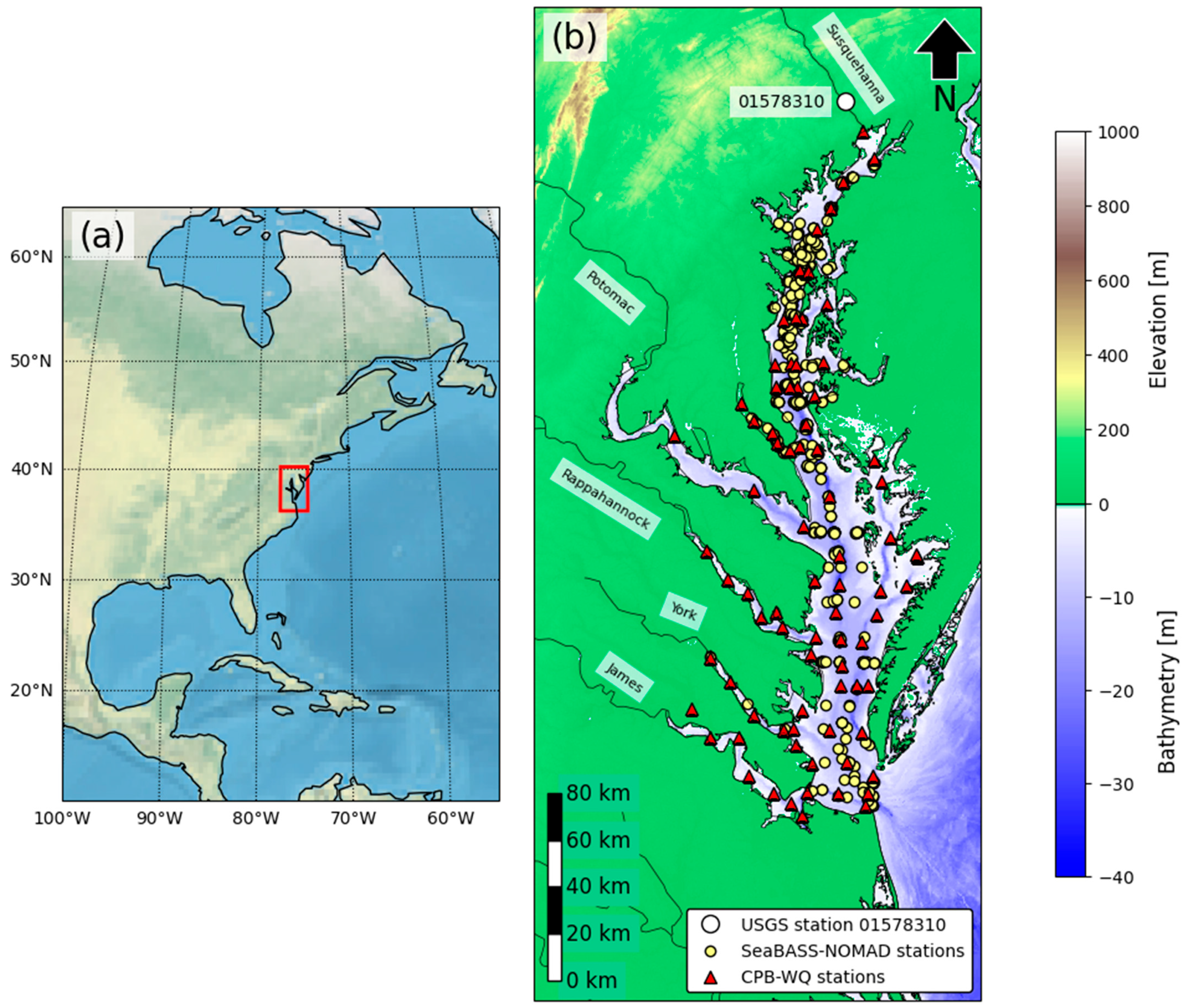
2.1. Study Area: Chesapeake Bay
2.2. Field Data
2.3. Satellite Data
2.4. Extra-Trees Machine Learning
2.5. Accuracy Metrics and Statistical Methods of Data Analysis
3. Results
3.1. Accuracy of Extra-Trees Machine Learning Models Predicting Chl-a in the Chesapeake Bay
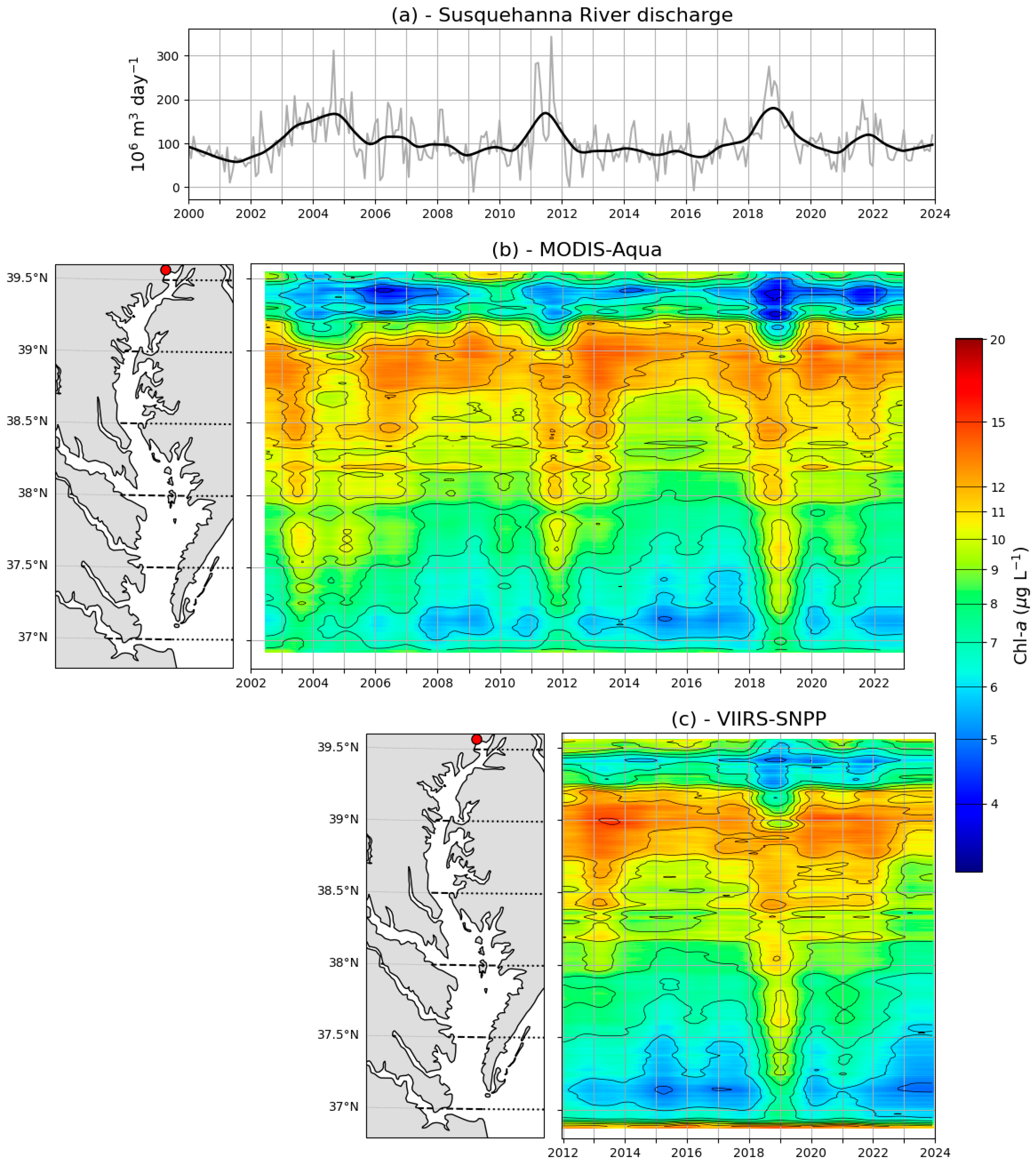
3.2. Spatiotemporal Variations of Chl-a Predicted from Satellite Imagery
4. Discussion
4.1. Model Performance
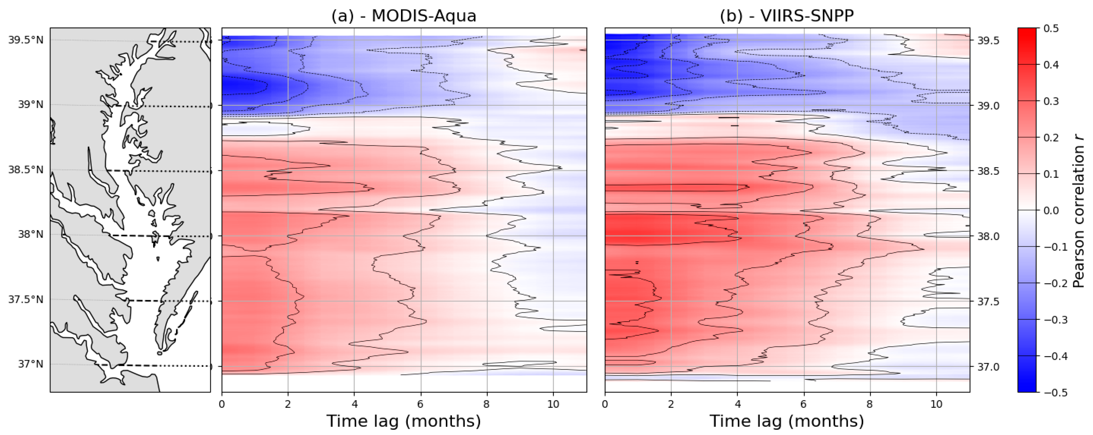
4.2. Spatiotemporal Variations of Satellite-Derived Chl-a in the Chesapeake Bay
5. Conclusions
Supplementary Materials
Author Contributions
Funding
Data Availability Statement
Acknowledgments
Conflicts of Interest
References
- IOCCG. Why Ocean Colour? The Societal Benefits of Ocean-Colour Technology; International Ocean-Colour Coordinating Group (IOCCG): Dartmouth, NS, Canada, 2008; p. 141. [Google Scholar]
- Carlson, R.E. A trophic state index for lakes. Limnol. Oceanogr. 1977, 22, 361–369. [Google Scholar] [CrossRef]
- Muller-Karger, F.E.; Kavanaugh, M.T.; Montes, E.; Balch, W.M.; Breitbart, M.; Chavez, F.P.; Doney, S.C.; Johns, E.M.; Letelier, R.M.; Lomas, M.W.; et al. A Framework for a Marine Biodiversity Observing Network Within Changing Continental Shelf Seascapes. Oceanography 2014, 27, 18–23. [Google Scholar] [CrossRef]
- Behrenfeld, M.J.; O’Malley, R.T.; Siegel, D.A.; McClain, C.R.; Sarmiento, J.L.; Feldman, G.C.; Milligan, A.J.; Falkowski, P.G.; Letelier, R.M.; Boss, E.S. Climate-driven trends in contemporary ocean productivity. Nature 2006, 444, 752–755. [Google Scholar] [CrossRef]
- Chavez, F.P.; Messié, M.; Pennington, J.T. Marine Primary Production in Relation to Climate Variability and Change. Annu. Rev. Mar. Sci. 2011, 3, 227–260. [Google Scholar] [CrossRef]
- Wang, H.; Convertino, M. Algal bloom ties: Systemic biogeochemical stress and Chlorophyll-a shift forecasting. Ecol. Indic. 2023, 154, 110760. [Google Scholar] [CrossRef]
- Bojinski, S.; Verstraete, M.; Peterson, T.C.; Richter, C.; Simmons, A.; Zemp, M. The Concept of Essential Climate Variables in Support of Climate Research, Applications, and Policy. Bull. Am. Meteorol. Soc. 2014, 95, 1431–1443. [Google Scholar] [CrossRef]
- GCOS. Systematic Observation Requirements for Satellite-Based Products for Climate. 2011 Update; Global Climate Observing System, World Meteorological Organization: Geneva, Switzerland, 2011; p. 138. [Google Scholar]
- Gordon, H.R.; Morel, A.Y. Remote Assessment of Ocean Color for Interpretation of Satellite Visible Imagery: A Review; Springer: Berlin/Heidelberg, Germany, 1983; p. 114. [Google Scholar] [CrossRef]
- Morel, A. Optical modeling of the upper ocean in relation to its biogenous matter content (case I waters). J. Geophys. Res. Oceans 1988, 93, 10749–10768. [Google Scholar] [CrossRef]
- Morel, A.; Prieur, L. Analysis of variations in ocean color. Limnol. Oceanogr. 1977, 22, 709–722. [Google Scholar] [CrossRef]
- Werdell, P.J.; Bailey, S.W.; Franz, B.A.; Harding, L.W.; Feldman, G.C.; McClain, C.R. Regional and seasonal variability of chlorophyll-a in Chesapeake Bay as observed by SeaWiFS and MODIS-Aqua. Remote Sens. Environ. 2009, 113, 1319–1330. [Google Scholar] [CrossRef]
- Gordon, H.R.; Wang, M. Retrieval of water-leaving radiance and aerosol optical thickness over the oceans with SeaWiFS: A preliminary algorithm. Appl. Opt. 1994, 33, 443–452. [Google Scholar] [CrossRef]
- Gordon, H.R. Atmospheric correction of ocean color imagery in the Earth Observing System era. J. Geophys. Res. Atmos. 1997, 102, 17081–17106. [Google Scholar] [CrossRef]
- Son, S.; Wang, M. Water properties in Chesapeake Bay from MODIS-Aqua measurements. Remote Sens. Environ. 2012, 123, 163–174. [Google Scholar] [CrossRef]
- Gitelson, A.A.; Schalles, J.F.; Hladik, C.M. Remote chlorophyll-a retrieval in turbid, productive estuaries: Chesapeake Bay case study. Remote Sens. Environ. 2007, 109, 464–472. [Google Scholar] [CrossRef]
- Magnuson, A.; Harding, L.W.; Mallonee, M.E.; Adolf, J.E. Bio-optical model for Chesapeake Bay and the Middle Atlantic Bight. Estuar. Coast. Shelf Sci. 2004, 61, 403–424. [Google Scholar] [CrossRef]
- Tzortziou, M.; Subramaniam, A.; Herman, J.R.; Gallegos, C.L.; Neale, P.J.; Harding, L.W. Remote sensing reflectance and inherent optical properties in the mid Chesapeake Bay. Estuar. Coast. Shelf Sci. 2007, 72, 16–32. [Google Scholar] [CrossRef]
- Le, C.; Hu, C.; Cannizzaro, J.; English, D.; Muller-Karger, F.; Lee, Z. Evaluation of chlorophyll-a remote sensing algorithms for an optically complex estuary. Remote Sens. Environ. 2013, 129, 75–89. [Google Scholar] [CrossRef]
- Ondrusek, M.; Stengel, E.; Kinkade, C.S.; Vogel, R.L.; Keegstra, P.; Hunter, C.; Kim, C. The development of a new optical total suspended matter algorithm for the Chesapeake Bay. Remote Sens. Environ. 2012, 119, 243–254. [Google Scholar] [CrossRef]
- Abbas, M.M.; Melesse, A.M.; Scinto, L.J.; Rehage, J.S. Satellite Estimation of Chlorophyll-a Using Moderate Resolution Imaging Spectroradiometer (MODIS) Sensor in Shallow Coastal Water Bodies: Validation and Improvement. Water 2019, 11, 1621. [Google Scholar] [CrossRef]
- Gilerson, A.A.; Gitelson, A.A.; Zhou, J.; Gurlin, D.; Moses, W.; Ioannou, I.; Ahmed, S.A. Algorithms for remote estimation of chlorophyll-a in coastal and inland waters using red and near infrared bands. Opt. Express 2010, 18, 24109–24125. [Google Scholar] [CrossRef]
- Mishra, S.; Mishra, D.R. Normalized difference chlorophyll index: A novel model for remote estimation of chlorophyll-a concentration in turbid productive waters. Remote Sens. Environ. 2012, 117, 394–406. [Google Scholar] [CrossRef]
- Harding, L.W.; Magnuson, A.; Mallonee, M.E. SeaWiFS retrievals of chlorophyll in Chesapeake Bay and the mid-Atlantic bight. Estuar. Coast. Shelf Sci. 2005, 62, 75–94. [Google Scholar] [CrossRef]
- Dall’Olmo, G.; Gitelson, A.A.; Rundquist, D.C. Towards a unified approach for remote estimation of chlorophyll-a in both terrestrial vegetation and turbid productive waters. Geophys. Res. Lett. 2003, 30, 18. [Google Scholar] [CrossRef]
- Gilerson, A.; Malinowski, M.; Agagliate, J.; Herrera-Estrella, E.; Tzortziou, M.; Tomlinson, M.C.; Meredith, A.; Stumpf, R.P.; Ondrusek, M.; Jiang, L.; et al. Development of VIIRS-OLCI chlorophyll-a product for the coastal estuaries. Front. Mar. Sci. 2024, 11, 1476425. [Google Scholar] [CrossRef]
- Hieronymi, M.; Müller, D.; Doerffer, R. The OLCI Neural Network Swarm (ONNS): A Bio-Geo-Optical Algorithm for Open Ocean and Coastal Waters. Front. Mar. Sci. 2017, 4, 140. [Google Scholar] [CrossRef]
- Pahlevan, N.; Smith, B.; Schalles, J.; Binding, C.; Cao, Z.; Ma, R.; Alikas, K.; Kangro, K.; Gurlin, D.; Hà, N.; et al. Seamless retrievals of chlorophyll-a from Sentinel-2 (MSI) and Sentinel-3 (OLCI) in inland and coastal waters: A machine-learning approach. Remote Sens. Environ. 2020, 240, 111604. [Google Scholar] [CrossRef]
- Cao, Z.; Wang, M.; Ma, R.; Zhang, Y.; Duan, H.; Jiang, L.; Xue, K.; Xiong, J.; Hu, M. A decade-long chlorophyll-a data record in lakes across China from VIIRS observations. Remote Sens. Environ. 2024, 301, 113953. [Google Scholar] [CrossRef]
- Salah, M.; Salem, S.I.; Utsumi, N.; Higa, H.; Ishizaka, J.; Oki, K. 3LATNet: Attention based deep learning model for global Chlorophyll-a retrieval from GCOM-C satellite. ISPRS J. Photogramm. Remote Sens. 2025, 220, 490–508. [Google Scholar] [CrossRef]
- Salah, M.; Higa, H.; Ishizaka, J.; Salem, S.I. 1D Convolutional Neural Network-based Chlorophyll-a Retrieval Algorithm for Sentinel-2 MultiSpectral Instrument in Various Trophic States. Sens. Mater. 2023, 35, 3743–3761. [Google Scholar] [CrossRef]
- Chen, S.; Hu, C.; Barnes, B.B.; Wanninkhof, R.; Cai, W.-J.; Barbero, L.; Pierrot, D. A machine learning approach to estimate surface ocean pCO2 from satellite measurements. Remote Sens. Environ. 2019, 228, 203–226. [Google Scholar] [CrossRef]
- El-Habashi, A.; Ahmed, S.; Ondrusek, M.; Lovko, V. Analyses of satellite ocean color retrievals show advantage of neural network approaches and algorithms that avoid deep blue bands. J. Appl. Remote Sens. 2019, 13, 024509. [Google Scholar] [CrossRef]
- Ahmad, M.W.; Mourshed, M.; Rezgui, Y. Trees vs Neurons: Comparison between random forest and ANN for high-resolution prediction of building energy consumption. Energy Build. 2017, 147, 77–89. [Google Scholar] [CrossRef]
- Nawar, S.; Mouazen, A.M. Comparison between Random Forests, Artificial Neural Networks and Gradient Boosted Machines Methods of On-Line Vis-NIR Spectroscopy Measurements of Soil Total Nitrogen and Total Carbon. Sensors 2017, 17, 2428. [Google Scholar] [CrossRef] [PubMed]
- Breiman, L. Random forests. Mach. Learn. 2001, 45, 5–32. [Google Scholar] [CrossRef]
- Banerjee, M.; Ding, Y.; Noone, A.M. Identifying representative trees from ensembles. Stat. Med. 2012, 31, 1601–1616. [Google Scholar] [CrossRef]
- Geurts, P.; Ernst, D.; Wehenkel, L. Extremely randomized trees. Mach. Learn. 2006, 63, 3–42. [Google Scholar] [CrossRef]
- Salomonson, V.V.; Barnes, W.L.; Maymon, P.W.; Montgomery, H.E.; Ostrow, H. MODIS: Advanced facility instrument for studies of the Earth as a system. IEEE Trans. Geosci. Remote Sens. 1989, 27, 145–153. [Google Scholar] [CrossRef]
- Goldberg, M.D.; Kilcoyne, H.; Cikanek, H.; Mehta, A. Joint Polar Satellite System: The United States next generation civilian polar-orbiting environmental satellite system. J. Geophys. Res. Atmos. 2013, 118, 13463–13475. [Google Scholar] [CrossRef]
- Cerco, C.F.; Cole, T. Three-Dimensional Eutrophication Model of Chesapeake Bay. J. Environ. Eng. 1993, 119, 1006–1025. [Google Scholar] [CrossRef]
- Du, J.; Shen, J. Water residence time in Chesapeake Bay for 1980–2012. J. Mar. Syst. 2016, 164, 101–111. [Google Scholar] [CrossRef]
- Zhong, L.; Li, M. Tidal energy fluxes and dissipation in the Chesapeake Bay. Cont. Shelf Res. 2006, 26, 752–770. [Google Scholar] [CrossRef]
- Zhong, L.; Li, M.; Foreman, M.G.G. Resonance and sea level variability in Chesapeake Bay. Cont. Shelf Res. 2008, 28, 2565–2573. [Google Scholar] [CrossRef]
- Shi, W.; Wang, M.; Jiang, L. Tidal effects on ecosystem variability in the Chesapeake Bay from MODIS-Aqua. Remote Sens. Environ. 2013, 138, 65–76. [Google Scholar] [CrossRef]
- Boesch, D.F.; Brinsfield, R.B.; Magnien, R.E. Chesapeake Bay eutrophication: Scientific understanding, ecosystem restoration, and challenges for agriculture. J. Environ. Qual. 2001, 30, 303–320. [Google Scholar] [CrossRef]
- Harding, L.W.; Mallonee, M.E.; Perry, E.S.; Miller, W.D.; Adolf, J.E.; Gallegos, C.L.; Paerl, H.W. Long-term trends, current status, and transitions of water quality in Chesapeake Bay. Sci. Rep. 2019, 9, 6709. [Google Scholar] [CrossRef]
- Harding, L.W.; Perry, E.S. Long-term increase of phytoplankton biomass in Chesapeake Bay, 1950–1994. Mar. Ecol. Prog. Ser. 1997, 157, 39–52. [Google Scholar] [CrossRef]
- Kemp, W.M.; Boynton, W.; Adolf, J.; Boesch, D.; Boicourt, W.; Brush, G.; Cornwell, J.; Fisher, T.; Glibert, P.; Hagy Iii, J.; et al. Eutrophication of Chesapeake Bay: Historical Trends and Ecological Interactions. Mar. Ecol. Prog. Ser. 2005, 303, 1–29. [Google Scholar] [CrossRef]
- Murphy, R.R.; Kemp, W.M.; Ball, W.P. Long-Term Trends in Chesapeake Bay Seasonal Hypoxia, Stratification, and Nutrient Loading. Estuaries Coasts 2011, 34, 1293–1309. [Google Scholar] [CrossRef]
- Borum, J. Shallow Waters and Land/Sea Boundaries. In Eutrophication in Coastal Marine Ecosystems; American Geophysical Union: Washington, DC, USA, 1996; pp. 179–203. [Google Scholar]
- Nixon, S.W.; Ammerman, J.W.; Atkinson, L.P.; Berounsky, V.M.; Billen, G.; Boicourt, W.C.; Boynton, W.R.; Church, T.M.; Ditoro, D.M.; Elmgren, R.; et al. The fate of nitrogen and phosphorus at the land-sea margin of the North Atlantic Ocean. Biogeochemistry 1996, 35, 141–180. [Google Scholar] [CrossRef]
- Kemp, W.M.; Smith, E.M.; Marvin-DiPasquale, M.; Boynton, W.R. Organic carbon balance and net ecosystem metabolism in Chesapeake Bay. Mar. Ecol. Prog. Ser. 1997, 150, 229–248. [Google Scholar] [CrossRef]
- Schubel, J.R.; Pritchard, D.W. Responses of upper Chesapeake Bay to variations in discharge of the Susquehanna River. Estuaries 1986, 9, 236–249. [Google Scholar] [CrossRef]
- Gallegos, C.L.; Werdell, P.J.; McClain, C.R. Long-term changes in light scattering in Chesapeake Bay inferred from Secchi depth, light attenuation, and remote sensing measurements. J. Geophys. Res. Oceans 2011, 116, C7. [Google Scholar] [CrossRef]
- Werdell, P.J.; Bailey, S.W. An improved in-situ bio-optical data set for ocean color algorithm development and satellite data product validation. Remote Sens. Environ. 2005, 98, 122–140. [Google Scholar] [CrossRef]
- Mueller, J.; Fargion, G.; McClain, C.; Pegau, W.; Zanefeld, J.; Mitchell, B.; Kahru, M.; Wieland, J.; Stramska, M. Ocean Optics Protocols for Satellite Ocean Color Sensor Validation, Rev. 4, Vol. IV: Inherent Optical Properties: Instruments, Characterisations, Field Measurements and Data Analysis Protocols; Goddard Space Flight Space Center: Greenbelt, MD, USA, 2003. [Google Scholar]
- Hu, C.; Feng, L.; Lee, Z.; Franz, B.A.; Bailey, S.W.; Werdell, P.J.; Proctor, C.W. Improving Satellite Global Chlorophyll a Data Products Through Algorithm Refinement and Data Recovery. J. Geophys. Res. Oceans 2019, 124, 1524–1543. [Google Scholar] [CrossRef]
- O’Reilly, J.E.; Maritorena, S.; Mitchell, B.G.; Siegel, D.A.; Carder, K.L.; Garver, S.A.; Kahru, M.; McClain, C. Ocean color chlorophyll algorithms for SeaWiFS. J. Geophys. Res. Oceans 1998, 103, 24937–24953. [Google Scholar] [CrossRef]
- Olson, M. Guide to Using Chesapeake Bay Program Water Quality Monitoring Data (EPA 903-R-12-001); Chesapeake Bay Program: Annapolis, MD, USA, 2012; pp. 1–155. [Google Scholar]
- D3731-20; Standard Practices for Measurement of Chlorophyll Content of Algae in Surface Waters. ASTM: West Conshohocken, PA, USA, 2020.
- Campbell, J.W. The lognormal distribution as a model for bio-optical variability in the sea. J. Geophys. Res. Oceans 1995, 100, 13237–13254. [Google Scholar] [CrossRef]
- US Geological Survey. National Water Information System Data Available on the World Wide Web (USGS Water Data for the Nation); US Geological Survey: Reston, VA, USA, 2016. [Google Scholar] [CrossRef]
- Bailey, S.W.; Werdell, P.J. A multi-sensor approach for the on-orbit validation of ocean color satellite data products. Remote Sens. Environ. 2006, 102, 12–23. [Google Scholar] [CrossRef]
- Geurts, P.; Louppe, G. Learning to rank with extremely randomized trees. PMLR 2011, 14, 49–61. [Google Scholar]
- Camana Acosta, M.R.; Ahmed, S.; Garcia, C.E.; Koo, I. Extremely Randomized Trees-Based Scheme for Stealthy Cyber-Attack Detection in Smart Grid Networks. IEEE Access 2020, 8, 19921–19933. [Google Scholar] [CrossRef]
- Smith, D.; Yenduri, S.; Iqbal, S.; Krishna, P.V. An efficient distributed protein disorder prediction with pasted samples. Comput. Electr. Eng. 2018, 65, 342–356. [Google Scholar] [CrossRef]
- Adams, S.; Choudhary, C.; De Cock, M.; Dowsley, R.; Melanson, D.; Nascimento, A.C.A.; Railsback, D.; Shen, J. Privacy-preserving training of tree ensembles over continuous data. Proc. Priv. Enhancing Technol. 2021, 2022, 205–226. [Google Scholar] [CrossRef]
- Ghazwani, M.; Begum, M.Y. Computational intelligence modeling of hyoscine drug solubility and solvent density in supercritical processing: Gradient boosting, extra trees, and random forest models. Sci. Rep. 2023, 13, 10046. [Google Scholar] [CrossRef] [PubMed]
- Götz, M.; Weber, C.; Blöcher, J.; Stieltjes, B.; Meinzer, H.-P.; Maier-Hein, K. Extremely randomized trees based brain tumor segmentation. In Proceedings of the MICCAI Workshop: Brain Tumor Segmentation (BraTS) 2014, Boston, MA, USA, 14 September 2014. [Google Scholar]
- Lawson, E.; Smith, D.; Sofge, D.; Elmore, P.; Petry, F. Decision forests for machine learning classification of large, noisy seafloor feature sets. Comput. Geosci. 2017, 99, 116–124. [Google Scholar] [CrossRef]
- Pedregosa, F.; Varoquaux, G.; Gramfort, A.; Michel, V.; Thirion, B.; Grisel, O.; Blondel, M.; Prettenhofer, P.; Weiss, R.; Dubourg, V. Scikit-learn: Machine learning in Python. J. Mach. Learn. Res. 2011, 12, 2825–2830. [Google Scholar]
- Seegers, B.N.; Stumpf, R.P.; Schaeffer, B.A.; Loftin, K.A.; Werdell, P.J. Performance metrics for the assessment of satellite data products: An ocean color case study. Opt. Express 2018, 26, 7404–7422. [Google Scholar] [CrossRef]
- Wynne, T.T.; Mishra, S.; Meredith, A.; Litaker, R.W.; Stumpf, R.P. Intercalibration of MERIS, MODIS, and OLCI Satellite Imagers for Construction of Past, Present, and Future Cyanobacterial Biomass Time Series. Remote Sens. 2021, 13, 2305. [Google Scholar] [CrossRef]
- Wynne, T.T.; Tomlinson, M.C.; Briggs, T.O.; Mishra, S.; Meredith, A.; Vogel, R.L.; Stumpf, R.P. Evaluating the Efficacy of Five Chlorophyll-a Algorithms in Chesapeake Bay (USA) for Operational Monitoring and Assessment. J. Mar. Sci. Eng. 2022, 10, 1104. [Google Scholar] [CrossRef]
- Glover, D.M.; Jenkins, W.J.; Doney, S.C. Modeling Methods for Marine Science; Cambridge University Press: Cambridge, UK, 2011. [Google Scholar]
- Sokal, R.; Rohlf, F. Biometry: The Principles and Practice of Statistics in Biological Research, 2nd ed.; W.H. Freeman and Company: New York, NY, USA, 2012; Volume 133. [Google Scholar]
- Brewin, R.J.W.; Sathyendranath, S.; Müller, D.; Brockmann, C.; Deschamps, P.-Y.; Devred, E.; Doerffer, R.; Fomferra, N.; Franz, B.; Grant, M.; et al. The Ocean Colour Climate Change Initiative: III. A round-robin comparison on in-water bio-optical algorithms. Remote Sens. Environ. 2015, 162, 271–294. [Google Scholar] [CrossRef]
- Wang, M.; Son, S.; Shi, W. Evaluation of MODIS SWIR and NIR-SWIR atmospheric correction algorithms using SeaBASS data. Remote Sens. Environ. 2009, 113, 635–644. [Google Scholar] [CrossRef]
- Azcarate, A.; Barth, A.; Sirjacobs, D.; Lenartz, F.; Beckers, J.-M. Data Interpolating Empirical Orthogonal Functions (DINEOF): A tool for geophysical data analyses. Mediter. Mar. Sci. 2011, 12, 5–11. [Google Scholar] [CrossRef]
- Beckers, J.M.; Rixen, M. EOF Calculations and Data Filling from Incomplete Oceanographic Datasets. J. Atmos. Ocean. Technol. 2003, 20, 1839–1856. [Google Scholar] [CrossRef]
- Liu, X.; Wang, M. Global daily gap-free ocean color products from multi-satellite measurements. Int. J. Appl. Earth Obs. Geoinf. 2022, 108, 102714. [Google Scholar] [CrossRef]
- Cleveland, R.B.; Cleveland, W.S.; McRae, J.E.; Terpenning, I. STL: A seasonal-trend decomposition procedure based on loess. J. Off. Stat. 1990, 6, 3–73. [Google Scholar]
- Vantrepotte, V.; Mélin, F. Temporal variability of 10-year global SeaWiFS time-series of phytoplankton chlorophyll a concentration. ICES J. Mar. Sci. 2009, 66, 1547–1556. [Google Scholar] [CrossRef]
- Cleveland, W.S. Robust Locally Weighted Regression and Smoothing Scatterplots. J. Am. Stat. Assoc. 1979, 74, 829–836. [Google Scholar] [CrossRef]
- Stock, A. Spatiotemporal distribution of labeled data can bias the validation and selection of supervised learning algorithms: A marine remote sensing example. ISPRS J. Photogramm. Remote Sens. 2022, 187, 46–60. [Google Scholar] [CrossRef]
- Wang, D.; Tang, B.-H.; Li, Z.-L. Evaluation of five atmospheric correction algorithms for multispectral remote sensing data over plateau lake. Ecol. Inform. 2024, 82, 102666. [Google Scholar] [CrossRef]
- Feng, L.; Hu, C. Land adjacency effects on MODIS Aqua top-of-atmosphere radiance in the shortwave infrared: Statistical assessment and correction. J. Geophys. Res. Oceans 2017, 122, 4802–4818. [Google Scholar] [CrossRef]
- Pahlevan, N.; Mangin, A.; Balasubramanian, S.V.; Smith, B.; Alikas, K.; Arai, K.; Barbosa, C.; Bélanger, S.; Binding, C.; Bresciani, M.; et al. ACIX-Aqua: A global assessment of atmospheric correction methods for Landsat-8 and Sentinel-2 over lakes, rivers, and coastal waters. Remote Sens. Environ. 2021, 258, 112366. [Google Scholar] [CrossRef]
- Harding, L.W.; Mallonee, M.E.; Perry, E.S.; David Miller, W.; Adolf, J.E.; Gallegos, C.L.; Paerl, H.W. Seasonal to Inter-Annual Variability of Primary Production in Chesapeake Bay: Prospects to Reverse Eutrophication and Change Trophic Classification. Sci. Rep. 2020, 10, 2019. [Google Scholar] [CrossRef]
- Miller, W.D.; Harding, J.; Lawrence, W. Climate forcing of the spring bloom in Chesapeake Bay. Mar. Ecol. Prog. Ser. 2007, 331, 11–22. [Google Scholar] [CrossRef]
- Nezlin, N.P.; Testa, J.M.; Zheng, G.; DiGiacomo, P.M. Satellite observations estimating the effects of river discharge and wind-driven upwelling on phytoplankton dynamics in the Chesapeake Bay. Integr. Environ. Assess. Manag. 2022, 18, 921–938. [Google Scholar] [CrossRef] [PubMed]
- Lohrenz, S.E.; Weidemann, A.D.; Tuel, M. Phytoplankton spectral absorption as influenced by community size structure and pigment composition. J. Plankton Res. 2003, 25, 35–61. [Google Scholar] [CrossRef]
- Ciotti, Á.M.; Lewis, M.R.; Cullen, J.J. Assessment of the relationships between dominant cell size in natural phytoplankton communities and the spectral shape of the absorption coefficient. Limnol. Oceanogr. 2002, 47, 404–417. [Google Scholar] [CrossRef]
- Bricaud, A.; Claustre, H.; Ras, J.; Oubelkheir, K. Natural variability of phytoplanktonic absorption in oceanic waters: Influence of the size structure of algal populations. J. Geophys. Res. Oceans 2004, 109, C11. [Google Scholar] [CrossRef]
- Feng, L.; Hu, C.; Chen, X.; Tian, L.; Chen, L. Human induced turbidity changes in Poyang Lake between 2000 and 2010: Observations from MODIS. J. Geophys. Res. Oceans 2012, 117, C7. [Google Scholar] [CrossRef]
- Shen, M.; Luo, J.; Cao, Z.; Xue, K.; Qi, T.; Ma, J.; Liu, D.; Song, K.; Feng, L.; Duan, H. Random forest: An optimal chlorophyll-a algorithm for optically complex inland water suffering atmospheric correction uncertainties. J. Hydrol. 2022, 615, 128685. [Google Scholar] [CrossRef]
- Saeed, U.; Jan, S.U.; Lee, Y.-D.; Koo, I. Fault diagnosis based on extremely randomized trees in wireless sensor networks. Reliab. Eng. Syst. Saf. 2021, 205, 107284. [Google Scholar] [CrossRef]
- Im, G.; Lee, D.; Lee, S.; Lee, J.; Lee, S.; Park, J.; Heo, T.-Y. Estimating Chlorophyll-a Concentration from Hyperspectral Data Using Various Machine Learning Techniques: A Case Study at Paldang Dam, South Korea. Water 2022, 14, 4080. [Google Scholar] [CrossRef]
- Vanhellemont, Q.; Ruddick, K. Atmospheric correction of metre-scale optical satellite data for inland and coastal water applications. Remote Sens. Environ. 2018, 216, 586–597. [Google Scholar] [CrossRef]
- Zhao, D.; Feng, L.; Sun, K. Development of a Practical Atmospheric Correction Algorithm for Inland and Nearshore Coastal Waters. IEEE Trans. Geosci. Remote Sens. 2022, 60, 5402515. [Google Scholar] [CrossRef]
- Malone, T.C.; Kemp, W.M.; Ducklow, H.W.; Boynton, W.R.; Tuttle, J.H.; Jonas, R.B. Lateral variation in the production and fate of phytoplankton in a partially stratified estuary. Mar. Ecol. Prog. Ser. 1986, 32, 149–160. [Google Scholar] [CrossRef]
- Zheng, G.; DiGiacomo, P.M. Detecting phytoplankton diatom fraction based on the spectral shape of satellite-derived algal light absorption coefficient. Limnol. Oceanogr. 2018, 63, S85–S98. [Google Scholar] [CrossRef]
- Le, C.; Hu, C.; Cannizzaro, J.; Duan, H. Long-term distribution patterns of remotely sensed water quality parameters in Chesapeake Bay. Estuar. Coast. Shelf Sci. 2013, 128, 93–103. [Google Scholar] [CrossRef]
- Malone, T.C.; Crocker, L.H.; Pike, S.E.; Wendler, B.W. Influences of river flow on the dynamics of phytoplankton production in a partially stratified estuary. Mar. Ecol. Prog. Ser. 1988, 48, 235–249. [Google Scholar] [CrossRef]
- Acker, J.G.; Harding, L.W.; Leptoukh, G.; Zhu, T.; Shen, S. Remotely-sensed chl a at the Chesapeake Bay mouth is correlated with annual freshwater flow to Chesapeake Bay. Geophys. Res. Lett. 2005, 32, 5. [Google Scholar] [CrossRef]
- Miller, W.D.; Kimmel, D.G.; Harding, L.W., Jr. Predicting spring discharge of the Susquehanna River from a winter synoptic climatology for the eastern United States. Water Resour. Res. 2006, 42, 5. [Google Scholar] [CrossRef]
- Hagy, J.D.; Boynton, W.R.; Keefe, C.W.; Wood, K.V. Hypoxia in Chesapeake Bay, 1950–2001: Long-term change in relation to nutrient loading and river flow. Estuaries 2004, 27, 634–658. [Google Scholar] [CrossRef]
- Qin, Q.; Shen, J. Typical relationships between phytoplankton biomass and transport time in river-dominated coastal aquatic systems. Limnol. Oceanogr. 2021, 66, 3209–3220. [Google Scholar] [CrossRef]
- Lucas, L.V.; Deleersnijder, E. Timescale Methods for Simplifying, Understanding and Modeling Biophysical and Water Quality Processes in Coastal Aquatic Ecosystems: A Review. Water 2020, 12, 2717. [Google Scholar] [CrossRef]
- Scavia, D.; Field, J.C.; Boesch, D.F.; Buddemeier, R.W.; Burkett, V.; Cayan, D.R.; Fogarty, M.; Harwell, M.A.; Howarth, R.W.; Mason, C.; et al. Climate change impacts on U.S. Coastal and Marine Ecosystems. Estuaries 2002, 25, 149–164. [Google Scholar] [CrossRef]
- Fisher, T.R.; Peele, E.R.; Ammerman, J.W.; Harding, L.W., Jr. Nutrient limitation of phytoplankton in Chesapeake Bay. Mar. Ecol. Prog. Ser. 1992, 82, 51–63. [Google Scholar] [CrossRef]
- Fisher, T.R.; Gustafson, A.B.; Sellner, K.; Lacouture, R.; Haas, L.W.; Wetzel, R.L.; Magnien, R.; Everitt, D.; Michaels, B.; Karrh, R. Spatial and temporal variation of resource limitation in Chesapeake Bay. Mar. Biol. 1999, 133, 763–778. [Google Scholar] [CrossRef]
- Zhang, Q.; Fisher, T.R.; Trentacoste, E.M.; Buchanan, C.; Gustafson, A.B.; Karrh, R.; Murphy, R.R.; Keisman, J.; Wu, C.; Tian, R.; et al. Nutrient limitation of phytoplankton in Chesapeake Bay: Development of an empirical approach for water-quality management. Water Res. 2021, 188, 116407. [Google Scholar] [CrossRef]
- Jiang, L.; Xia, M. Wind effects on the spring phytoplankton dynamics in the middle reach of the Chesapeake Bay. Ecol. Model. 2017, 363, 68–80. [Google Scholar] [CrossRef]
- Schubel, J.R. Turbidity Maximum of the Northern Chesapeake Bay. Science 1968, 161, 1013–1015. [Google Scholar] [CrossRef]
- Zheng, G.; DiGiacomo, P.M.; Kaushal, S.S.; Yuen-Murphy, M.A.; Duan, S. Evolution of Sediment Plumes in the Chesapeake Bay and Implications of Climate Variability. Environ. Sci. Technol. 2015, 49, 6494–6503. [Google Scholar] [CrossRef]
- Harding, L. Long-term trends in the distribution of phytoplankton in Chesapeake Bay: Roles of light, nutrients and streamflow. Mar. Ecol. Prog. Ser. 1994, 104, 267–291. [Google Scholar] [CrossRef]
- Liu, X.; Wang, M. River runoff effect on the suspended sediment property in the upper Chesapeake Bay using MODIS observations and ROMS simulations. J. Geophys. Res. Oceans 2014, 119, 8646–8661. [Google Scholar] [CrossRef]
- Chen, B.; Cai, W.-J.; Brodeur, J.R.; Hussain, N.; Testa, J.M.; Ni, W.; Li, Q. Seasonal and spatial variability in surface CO and air–water CO flux in the Chesapeake Bay. Limnol. Oceanogr. 2020, 65, 3046–3065. [Google Scholar] [CrossRef]
- Jiang, L.; Xia, M. Dynamics of the Chesapeake Bay outflow plume: Realistic plume simulation and its seasonal and interannual variability. J. Geophys. Res. Oceans 2016, 121, 1424–1445. [Google Scholar] [CrossRef]
- Harding, L.W.; Gallegos, C.L.; Perry, E.S.; Miller, W.D.; Adolf, J.E.; Mallonee, M.E.; Paerl, H.W. Long-Term Trends of Nutrients and Phytoplankton in Chesapeake Bay. Estuaries Coasts 2016, 39, 664–681. [Google Scholar] [CrossRef]
- Turner, J.S.; Friedrichs, C.T.; Friedrichs, M.A.M. Long-Term Trends in Chesapeake Bay Remote Sensing Reflectance: Implications for Water Clarity. J. Geophys. Res. Oceans 2021, 126, e2021JC017959. [Google Scholar] [CrossRef]


| Data Source of Rrs | Chl-a Algorithm | ET Model Features | N 1 | R2 2 | MSE 3 | MAE 4 | MMB 5 | Slope 6 |
|---|---|---|---|---|---|---|---|---|
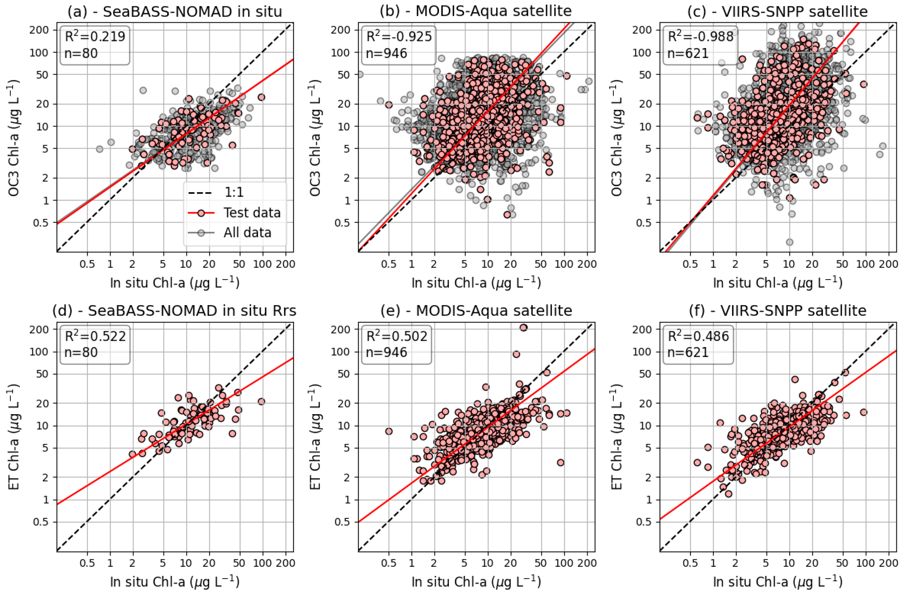
| In situ—test subset | ET | Rrs | 80 | 0.522 | 0.047 | 1.481 | 1.113 | 0.639 |
| In situ—test subset | ET | Rrs, Lat 7, DoY 8, Depth 9, Doff 10 | 80 | 0.475 | 0.069 | 1.554 | 1.031 | 0.720 |
| In situ—test subset | OC3 | 80 | 0.219 | 0.077 | 1.644 | 0.830 | 0.719 | |
| In situ—all data | OC3 | 399 | 0.100 | 0.096 | 1.765 | 0.763 | 0.711 | |
| MYD 11—test subset | ET | Rrs | 946 | 0.502 | 0.044 | 1.395 | 0.994 | 0.756 |
| MYD—test subset | ET | Rrs, Lat, DoY, Depth, Doff | 946 | 0.581 | 0.036 | 1.362 | 0.990 | 0.698 |
| MYD—test subset | OC3 | 946 | −0.925 | 0.169 | 2.087 | 1.562 | 1.115 | |
| MYD—all data | OC3 | 4729 | −0.903 | 0.165 | 2.066 | 1.556 | 1.057 | |
| VII 12—test subset | ET | Rrs | 621 | 0.486 | 0.044 | 1.409 | 0.995 | 0.735 |
| VII—test subset | ET | Rrs, Lat, DoY, Depth, Doff | 621 | 0.557 | 0.037 | 1.371 | 1.004 | 0.722 |
| VII—test subset | OC3 | 621 | −0.988 | 0.171 | 2.060 | 1.717 | 1.220 | |
| VII—all data | OC3 | 3104 | −1.251 | 0.190 | 2.159 | 1.741 | 1.237 |
| Data Source of Rrs | Standard OC3 Algorithms | Extra-Trees Machine Learning Models | ||||||
|---|---|---|---|---|---|---|---|---|
| Mean | St. Dev. | Median | IQR 1 | Mean | St. Dev. | Median | IQR 1 | |
| In situ | 0.941 | 0.314 | 0.885 | 0.338 | 1.056 | 0.286 | 1.002 | 0.245 |
| MODIS-Aqua | 1.375 | 1.443 | 1.202 | 0.499 | 1.107 | 1.195 | 1.000 | 0.217 |
| VIIRS-SNPP | 1.364 | 1.301 | 1.241 | 0.574 | 1.059 | 0.780 | 1.000 | 0.241 |
Disclaimer/Publisher’s Note: The statements, opinions and data contained in all publications are solely those of the individual author(s) and contributor(s) and not of MDPI and/or the editor(s). MDPI and/or the editor(s) disclaim responsibility for any injury to people or property resulting from any ideas, methods, instructions or products referred to in the content. |
© 2025 by the authors. Licensee MDPI, Basel, Switzerland. This article is an open access article distributed under the terms and conditions of the Creative Commons Attribution (CC BY) license (https://creativecommons.org/licenses/by/4.0/).
Share and Cite
Nezlin, N.P.; Son, S.; Salem, S.I.; Ondrusek, M.E. Chlorophyll-a in the Chesapeake Bay Estimated by Extra-Trees Machine Learning Modeling. Remote Sens. 2025, 17, 2151. https://doi.org/10.3390/rs17132151
Nezlin NP, Son S, Salem SI, Ondrusek ME. Chlorophyll-a in the Chesapeake Bay Estimated by Extra-Trees Machine Learning Modeling. Remote Sensing. 2025; 17(13):2151. https://doi.org/10.3390/rs17132151
Chicago/Turabian StyleNezlin, Nikolay P., SeungHyun Son, Salem I. Salem, and Michael E. Ondrusek. 2025. "Chlorophyll-a in the Chesapeake Bay Estimated by Extra-Trees Machine Learning Modeling" Remote Sensing 17, no. 13: 2151. https://doi.org/10.3390/rs17132151
APA StyleNezlin, N. P., Son, S., Salem, S. I., & Ondrusek, M. E. (2025). Chlorophyll-a in the Chesapeake Bay Estimated by Extra-Trees Machine Learning Modeling. Remote Sensing, 17(13), 2151. https://doi.org/10.3390/rs17132151