Range and Wave Height Corrections to Account for Ocean Wave Effects in SAR Altimeter Measurements Using Neural Network

Abstract

Compared to conventional pulse-limited altimeters (i.e., low-resolution mode, LRM), the synthetic aperture radar (SAR, i.e., high-resolution mode, HRM) altimeter offers superior precision and along-track resolution abilities. However, because the SAR altimeter relies on Doppler shifts caused by the relative movement between radar scattering points and the altimeter antenna, the geophysical parameters obtained by the SAR altimeter are sensitive to the direction of ocean wave movements driven by the wind and waves. Both practice and theory have shown that the wind and wave effects have a greater impact on HRM data than LRM. LRM values of range and significant wave height (SWH) from modern retracking are the best representations there are of these quantities, and this study aims to bring HRM data into line with them. In this study, wind and wave effects in SAR altimeter measurements were analyzed and corrected. The radar altimeter onboard the Sentinel-6 satellite is the first SAR altimeter to operate in an interleaved open burst mode. It has the capability of simultaneous generation of both LRM and HRM data. This study utilizes Sentinel-6 altimetry data and ERA5 re-analysis data to identify the influence of ocean waves. The analysis is based on the altimeter range and SWH differences between the HRM and LRM measurements with respect to different geophysical parameters derived from model data. Results show that both HRM range and SWH measurements are impacted by SWH and wind speed, and the HRM SWH measurements are also significantly impacted by vertical velocity. An upwave/downwave bias between HRM and LRM range is observed. To reduce wave impact on the SAR altimeter measurements, a back-propagation neural network (BPNN) method is proposed to correct the HRM range and SWH measurements. Based on Sentinel-6 measurements and ERA5 re-analysis data, our corrections significantly reduce biases between LRM and HRM range and SWH values. Finally, the accuracies of the sea surface height (SSH) and SWH measurements after correction are assessed using crossover analysis and compared against NDBC buoy data. The standard deviation (STD) of the HRM SSH differences at crossovers has no significant changes before (3.97 cm) and after (3.94 cm) correction. In comparison to the NDBC data, the root mean square error (RMSE) of the corrected HRM SWH data is 0.187 m, which is significantly better than that with no correction (0.265 m).

1. Introduction

The radar altimeter, operating as an active microwave remote sensor, is capable of continuously monitoring the oceans on a global scale. It measures key factors like sea surface height (SSH), significant wave height (SWH), and backscattering coefficient by retracking the altimeter waveforms. More than 20 radar altimetry satellites have been launched over the past few decades. Radar altimetry data have been widely used in research pertaining to ocean circulation [1,2], mesoscale eddies [3,4], global and regional sea level changes [5,6], ocean short-wave gravity field [7,8,9], seafloor topography [10,11], ocean tides [12,13], ice sheet elevation [14,15], sea-ice thickness [16,17,18], and inland water levels [19,20].

The conventional pulse-limited radar altimeter estimates the minimum radar range by employing echo delays from the pulse-limited footprint [21,22]. Its footprint is a circular area with a diameter of several kilometers, which increases as SWH grows. In the first few decades of altimetry, the conventional pulse-limited radar altimeters have demonstrated their significance in monitoring ocean parameters, including wind speed, SSH, and SWH, from satellites including ERS-1, ERS-2, Envisat, Topex/Poseidon, Jason-1/2/3 [23], SARAL/Altika and HY-2A/B/C/D [24,25]. As a result, they have become an essential tool for predicting oceans, analyzing climate and monitoring sea levels.

Due to the pulse-limited operating mechanism, the precision of conventional radar altimeters has been difficult to improve significantly after decades of development [26]. The restricted spatial resolution of conventional radar altimeters restricts their applicability in areas such as sea ice, inland and coastal regions. The SAR altimeters improve the azimuthal resolution to about 300 m [27] by Doppler sharpening and the resolution does not change with the change in SWH [28]. They improve the precision by delay compensation and multi-looking processing. Currently, the main altimetry satellites carrying SAR altimeters are Cryosat-2 [29], Sentinel-3A/B and Jason-CS/Sentinel-6 [30], and SAR altimetry data have been extensively utilized in ocean [31], sea ice [32], coastal [33,34] and inland [35] studies.

Questions about the observability of small-scale ocean phenomena arise as along-track resolution improves and noise of measurements is reduced. The SAR altimeter utilizes Doppler shifts resulting from the relative motion of the altimeter antenna and the radar scattering spots [30]. Therefore, the geophysical parameters retrieved from the SAR altimeter are influenced by the orientation of sea surface movements induced by winds and waves. Radar scatterers at all angles within the circular measuring zone are given equal weight by the conventional radar altimeter. In addition, wind vectors and sea state can have an impact on the radar cross-sections [36], which also indicates that sea surface motion affects SAR measurements. While SAR altimetry has been shown to provide more precise geophysical parameters compared to LRM altimetry, both retrieval methods can exhibit varying levels of accuracy and bias [32]. To ensure consistent continuity between SAR and conventional radar altimeter measurements, reducing the impact of ocean waves on SAR altimeter data is important.

The influence of waves on the Doppler signal has been a subject of discussion for a considerable period of time, with the effect arising from a variety of factors. In 2015, Aouf and Phalippou [37] demonstrated that the propagation direction of waves relative to the satellite orbit, as well as the period of waves, have a strong influence on the Doppler signal. Later, the impact of long waves was further investigated by Rieu et al. [38], Reale et al. [39], Moreau et al. [30] and Abdalla et al. [40]. In 2016, Boisot et al. [41] demonstrated that orbital velocities induced by the sea state (winds and swells), irrespective of their direction, have an effect on the Doppler signal. Further theoretical studies by Egido et al. [42], Amarouche et al. [43], Tran et al. [44] and Buchhaupt et al. [45] showed that the sea state can bias the estimation of the SWH, which in turn induces a bias in the sea surface height through sea state bias correction. In 2020, Tran et al. [44] used Sentinel-3 data to reconfirm the impact of wave period and wave direction on SAR altimeters and modeled the effect of wave direction. Quartly et al. [46] showed the clear difference between SAR (HRM) and PLRM estimates of wave height varied almost linearly with SWH. Amarouche et al. [47] investigated the impact of wind speed and vertical wave speed standard deviation on range and SWH using the Sentinel-6 altimetry data.

The radar altimeter aboard Sentinel-6 is the first SAR altimeter operating in an inter-leaved open burst mode. It can generate both LRM and HRM data concurrently, thus facilitating a comprehensive and direct examination of discrepancies between the two retrieval categories. To mitigate the discrepancies in parameters estimated from LRM and HRM data, Egido et al. [48] proposed a look-up table methodology for correcting HRM SWH data based on SWH and mean wave period. The application of this correction has been demonstrated to significantly reduce the bias between HRM and LRM SWH measurements, thereby reducing the SWH spectrum. Buchhaupt et al. [32] introduced a new SAR stack retracker, which provides estimates of SSH and SWH with excellent agreement when compared to LRM results. In order to achieve this objective, they additionally estimated the STD of the vertical wave particle velocity ${\sigma }_v$ and introduced a new metric $u_x$ associated with the residual Doppler in the echo, which correlates with the wind direction and wind speed.

In this study, we focus on analyzing the impact of ocean waves on the SAR altimeter measurements and reducing the inconsistencies between the HRM and LRM range and SWH measurements. The Sentinel-6 altimetry data and ERA5 re-analysis data are used to characterize the effect of ocean wave motion on SAR altimeter measurements. The analysis examines the altimeter range and SWH differences between the HRM and LRM measurements with respect to different geophysical parameters derived from model data. To reduce the inconsistencies between the HRM and LRM range and SWH measurements, we propose a BP neural network method to correct the HRM range and SWH measurements. The neural network is trained using ERA5 wave parameters (e.g., SWH, wave period, and wind speed) as input features and the bias between LRM and HRM range and SWH measurements as the target values. By learning the relationship between ocean wave conditions (characterized by ERA5 data) and the observed discrepancies (derived from LRM-HRM biases), the model predicts corrections for HRM range and SWH values, thereby effectively reducing biases between the two measurement modes. Finally, we assess the accuracies of the SSH and SWH measurements after correction by using crossover analysis and comparing them against the National Data Buoy Center (NDBC) buoy data, respectively.

2. Datasets

2.1. Sentinel-6 Altimetry Data

The Sentinel-6 satellite is equipped with the advanced Poseidon-4 radar altimeter for global and regional monitoring of variations in sea levels and the rate of rise. The Poseidon-4 radar altimeter is a dual-frequency device functioning at 5.4 GHz and 13.58 GHz. This altimeter is produced by THALES Alenia Space [49]. It is optimized on the basis of the Jason series, CryoSat-2, and Copernicus Sentinel-3 satellites [50], and combines dual-frequency (Ku-band and C-band) radar altimeter technology developed by ESA, which not only improves the accuracy and stability of the Jason series of radar altimeters but also inherits the high-resolution mode from CryoSat-2 and Sentinel-3. Poseidon-4 uses an interleaved open burst. More independent looks are obtained compared to the Sentinel-3A/B SAR altimeter and it can reduce the altimeter’s instrument noise. Poseidon-4’s design allows for the simultaneous acquisition of data in both HRM and LRM.

In this study, the range and SWH measurements from Sentinel-6 are derived from the operational Level-2 (L2) altimeter products. Poseidon-4 L2 products are categorized into three distinct types: near real-time (NRT), short time critical (STC), and non-time critical (NTC). We use products developed with the maximum latency (60 days, NTC) to obtain the most precise estimation of the orbit and geophysical corrections. In this experiment we used Ku-band radar altimeter data for a total of one year (February 2023–February 2024). We calculated the bias (i.e., HRM-LRM) from the Sentinel-6 L2 files produced by the F08 processing baseline.

Figure 1 shows histograms of the data distributions of range bias (i.e., HRM-LRM) and SWH bias, as well as the means and standard deviations, that we obtained using one year of Sentinel-6 data. This is the distribution of the dependent variable for the subsequent experiments we conducted.

2.2. ERA5 Re-Analysis Data

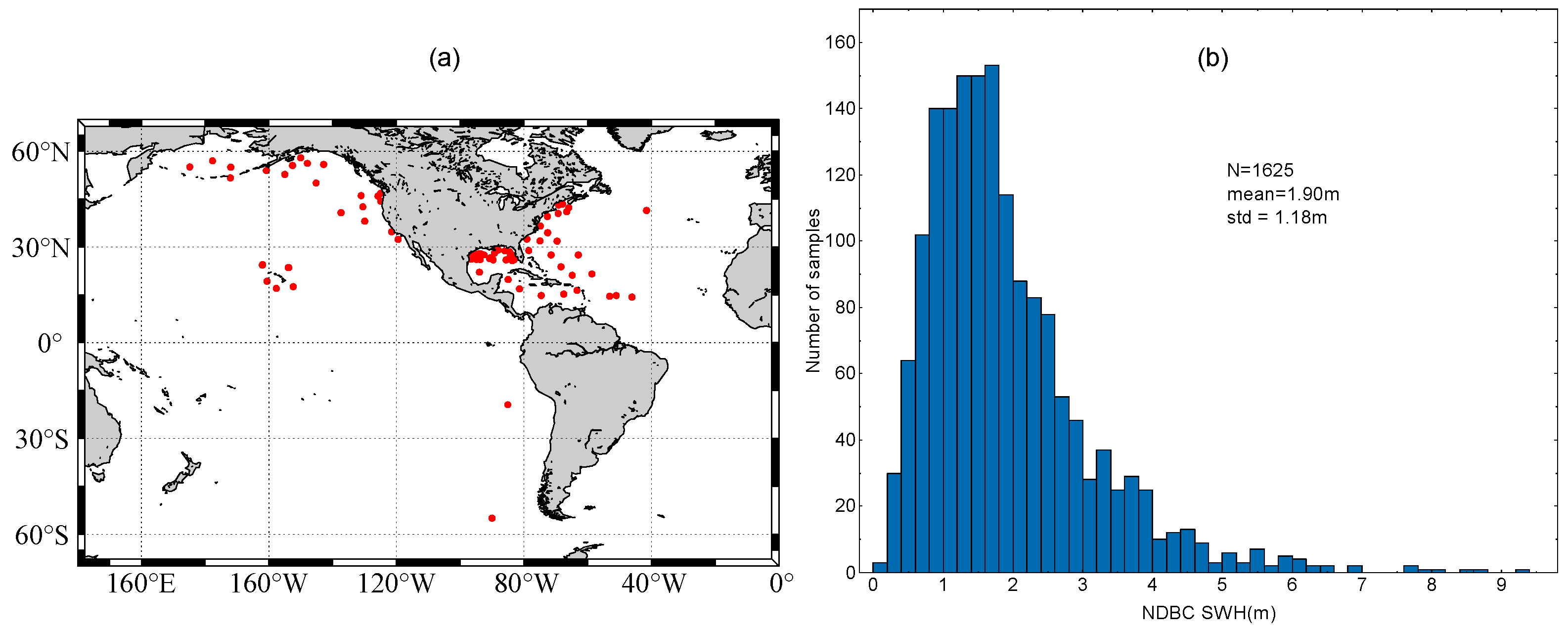
ERA5 is the fifth generation of European Centre for Medium-Range Weather Forecasts (ECMWF) re-analysis of worldwide climate and meteorological data spanning the last 80 years. Data are available from 1940 onwards. ERA5 is the successor to the ERA-Interim reanalysis. ERA-Interim’s spatial resolution is 0.75° and its temporal resolution is 6 h, whereas ERA5 has significantly enhanced spatial and temporal resolutions of 0.25° and 1 h, respectively.

We aim to examine the impact of ocean wave motion on range and SWH obtained from Sentinel-6 altimetry measurements. We use the following ocean wave parameters from the ERA5 dataset [51]: wind speed u/v component (u: −16–20 m/s, v: −18–17 m/s), mean wave period (MWP, 2–16 s), mean period of wind waves (MPWW, 1.45–12 s), mean period of total swell (MPTS, 2.5–15.5 s), wind direction, mean wave direction (MWD, 0–360°), mean direction of wind waves (MDWW, 0–360°), mean direction of total swell (MDTS, 0–360°) and significant height of combined wind waves and swell (SWH, 0–12 m). Figure 2 shows histograms of the data distributions of these parameters, as well as the means and standard deviations, where the wind speed and direction are calculated from the wind speed u/v component of ERA5, see Equations (1) and (3), and then subtracting 360° from the value of wind direction greater than 180° to make the range (−180°, 180°).

The ocean/sea surface wave field consists of a combination of waves with different heights, lengths and directions (known as the two-dimensional wave spectrum). The wave spectrum can be decomposed into wind-sea waves, which are directly affected by local winds, and swell, the waves that were generated by the wind at a different location and time.

Mean wave period (MWP) is the average time it takes for two consecutive wave crests, on the surface of the ocean/sea, to pass through a fixed point. It is the mean over all frequencies and directions of the two-dimensional wave spectrum. Mean period of wind waves (MPWW) is the average time it takes for two consecutive wave crests, on the surface of the ocean/sea generated by local winds, to pass through a fixed point. It is the mean over all frequencies and directions of the total wind-sea spectrum. Mean period of total swell (MPTS) is the average time it takes for two consecutive wave crests, on the surface of the ocean/sea associated with swell, to pass through a fixed point. It is the mean over all frequencies and directions of the total swell spectrum. Mean wave direction (MWD) is the mean direction of ocean/sea surface waves. It is the mean over all frequencies and directions of the two-dimensional wave spectrum. Mean direction of wind waves (MDWW) is the mean direction of waves generated by local winds. It is the mean over all frequencies and directions of the total wind–sea wave spectrum. Mean direction of total swell (MDTS) is the mean direction of waves associated with swell. It is the mean over all frequencies and directions of the total swell spectrum. The significant height of combined wind waves and swell (SWH) represents the average height of the highest third of surface ocean/sea waves generated by wind and swell. It represents the vertical distance between the wave crest and the wave trough. This parameter is four times the square root of the integral over all directions and all frequencies of the two-dimensional wave spectrum.

2.3. NDBC SWH Data

The hourly NDBC buoy data are used to assess the corrected Sentinel-6 HRM SWH measurements. To mitigate the impact of land influences, the analysis was conducted exclusively on buoys situated more than 50 km from the shoreline. The locations of the 78 buoys used in this study are illustrated in Figure 3.

3. Analysis of the Impact of Ocean Waves on the SAR Altimeter Measurements

According to previous studies, the technique of SAR altimetry employs the Doppler shifts that are generated by the relative movement between the altimeter antenna and the radar scattering spots on the ocean, potentially rendering SAR sensitive to wave motion. Conversely, LRM assigns uniform weight to radar scatterers situated at all angles inside a circular measuring zone. Therefore, LRM should be less affected by waves compared to HRM [32,44]. Results in Moreau et al. [30], and Jiang et al. [52] also show that the LRM data are less sensitive to wave direction, period, and vertical velocity than the SAR mode data. Therefore, we use the LRM measurements as a reference to analyze the effect of ocean waves on SAR altimeter measurements. Based on this, we use the HRM-LRM data, i.e., the deviation, as the object of study for the impact analysis in the subsequent experiments.

We employ Sentinel-6 altimetry data and external factors from wave models (ERA5) to analyze the behavior of range and significant wave height (SWH) estimates. The analysis is based on altimeter range and SWH, HRM and LRM differences concerning different geophysical parameters derived from model data.

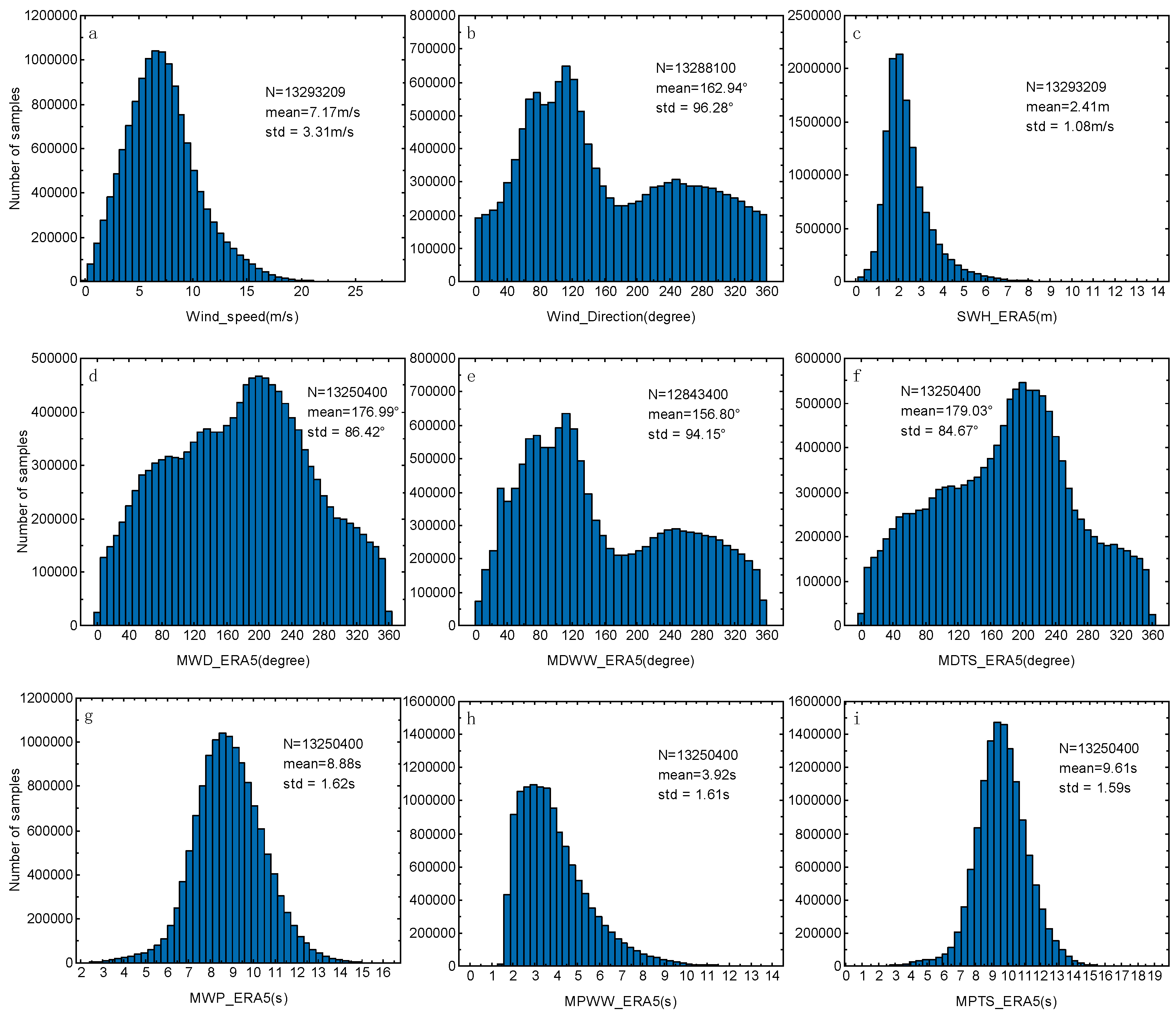
3.1. Computation of New Parameters from ERA5 Wave Model Parameters

In this study, the wave parameters derived from ERA5 we used are: relative wind direction (angle of wind direction relative to flight direction), wind speed projection, relative wave direction (angle of wave propagation direction relative to flight direction), relative mean wave direction, relative mean direction of wind waves, relative direction of total swell, and standard deviation of vertical velocity.

We know that the footprint of the SAR altimeter is strips along the satellite track direction, and in cross-track direction, it is the same as conventional radar altimeters. That means it is also insensitive to ocean fluctuations in the cross-track direction. Therefore, in this paper, we only study the parameters along the track direction which is the previously mentioned relative direction.

The relative wind direction here refers to the angle between the wind direction and the flight direction, which is calculated as follows (The direction of the north wind is defined as 0°, i.e., blowing from north to south and β as the angle between the satellite flight direction and due south):

$${\varphi }_{wind}=\mathrm{mod}(270-{\displaystyle \frac{180}{\pi }}\cdot \arctan 2(v,u),360)$$

(1)

$${\varphi }_{wind\_rel}=\mathrm{mod}({\varphi }_{wind}-\beta ,360)$$

(2)

where $v$ and $u$ are v-component and u-component of 10 m wind, respectively. ${\varphi }_{wind}$ and ${\varphi }_{wind\_rel}$ are the absolute direction of wind and relative wind direction, respectively.

The relative MWD, MDWW and MDTS are calculated in the same way as the relative wind direction.

The wind speed projection $V_{wind\_proj}$ (WSP) is the projected value of the wind speed $V_{wind}$ (WS) in the direction of the satellite’s flight, and the calculation is as follows:

$$V_{wind}=\sqrt{u^2+v^2}$$

(3)

$$V_{wind\_proj}=V_{wind}\cdot \mathit{cos}({\varphi }_{wind\_rel})$$

(4)

The STD of the vertical velocity of ocean waves is the degree of dispersion of the change in the velocity of the up and down motion of waves at the ocean surface over a given period. It reflects the strength and instability of the movement of waves in the vertical direction. The larger the standard deviation is, the more significant the change in the vertical speed of the wave, and the stronger the volatility; the smaller the standard deviation is, the smoother the wave movement is. Vertical velocity standard deviation is an important parameter describing the vertical movement of waves, which is related to the significant wave height $H_s$, wave period $T_{02}$, wave steepness ${\mu }_m$ and other parameters of the wave, so it can be calculated from the wave steepness as follows [48]:

$${\mu }_m={\displaystyle \frac{1}{\sqrt{2}\pi \left(1+{\upsilon }^2\right)g}}\cdot {\displaystyle \frac{{\sigma }_v^2}{\frac{H_s}{4}}}={\displaystyle \frac{2\pi H_s}{g{T}_{02}^2}}$$

(5)

This, in turn, gives the vertical velocity standard deviation ${\sigma }_v$ as:

$${\sigma }_v={\displaystyle \frac{\sqrt{1+{\upsilon }^2}}{2^{\frac{1}{4}}}}\cdot {\displaystyle \frac{\pi H_s}{T_{02}}}$$

(6)

where $\upsilon$ is a constant parameter in the spectral model, and $\upsilon =0.39$ for the JONSWAP spectrum and $\upsilon =0.425$ for the Pierson-Moskowitz spectrum.

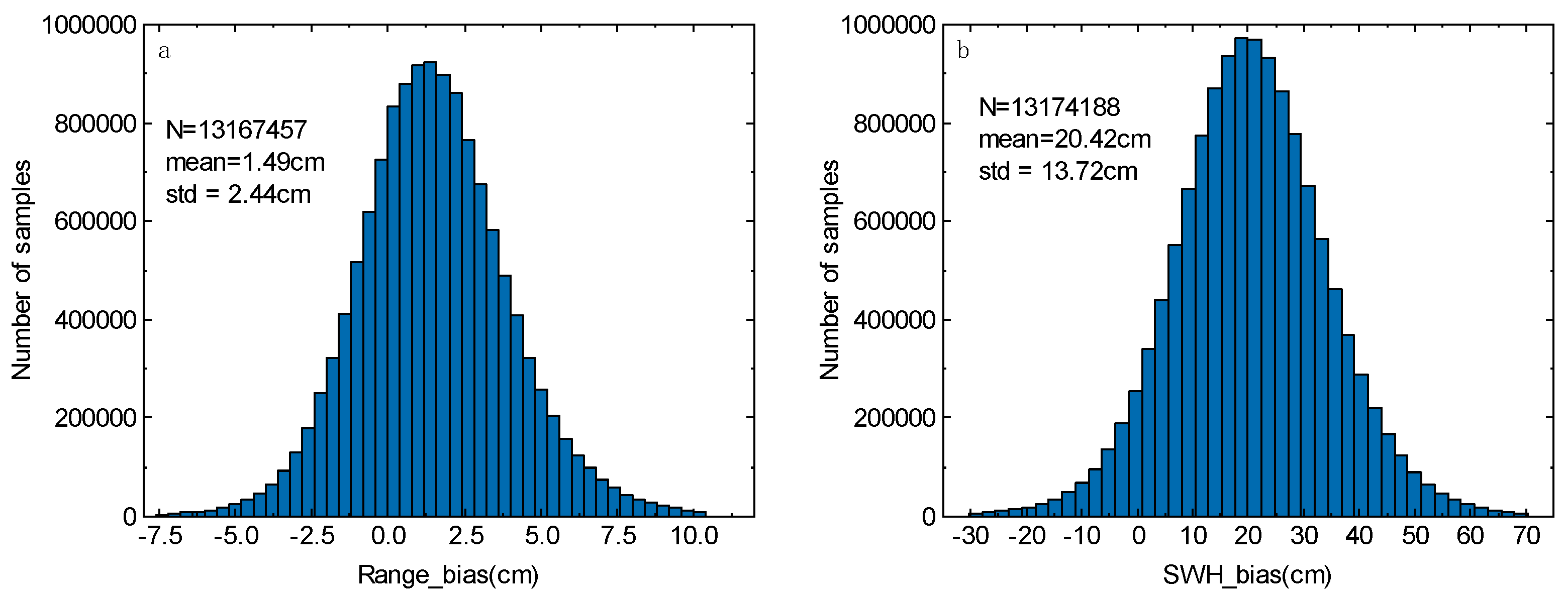
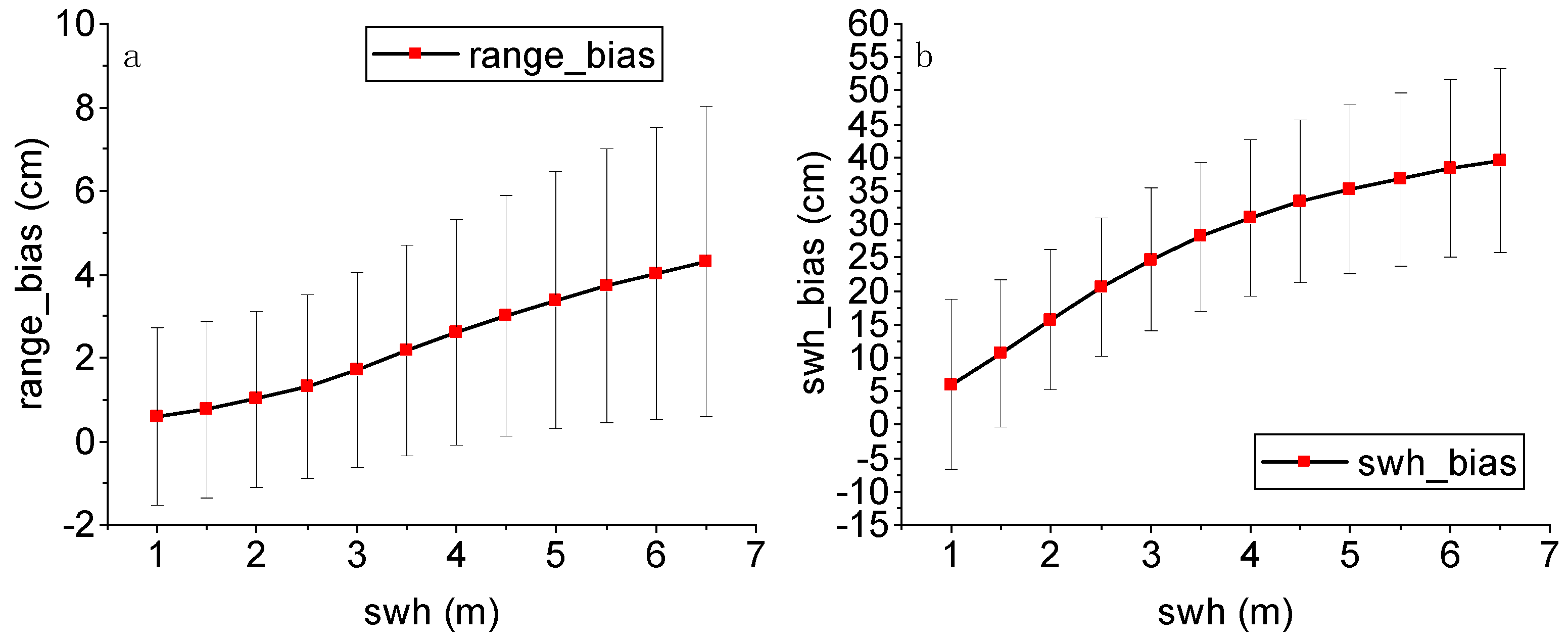
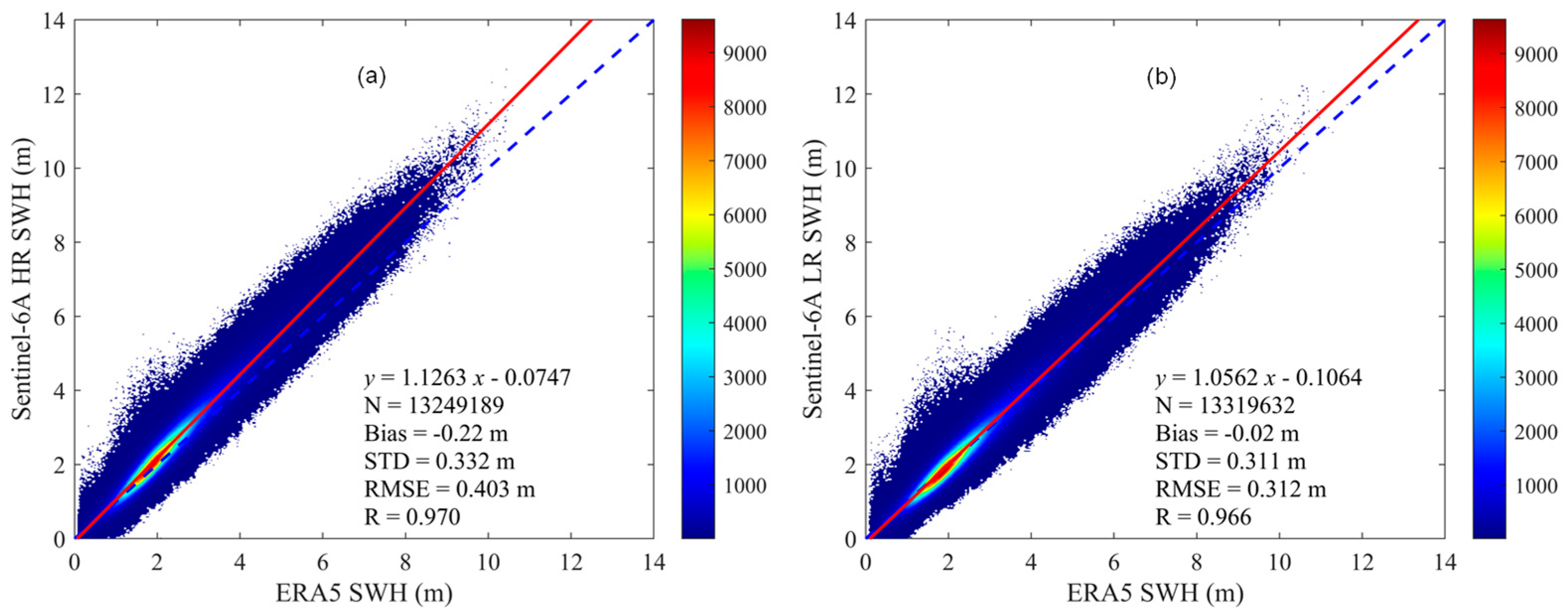
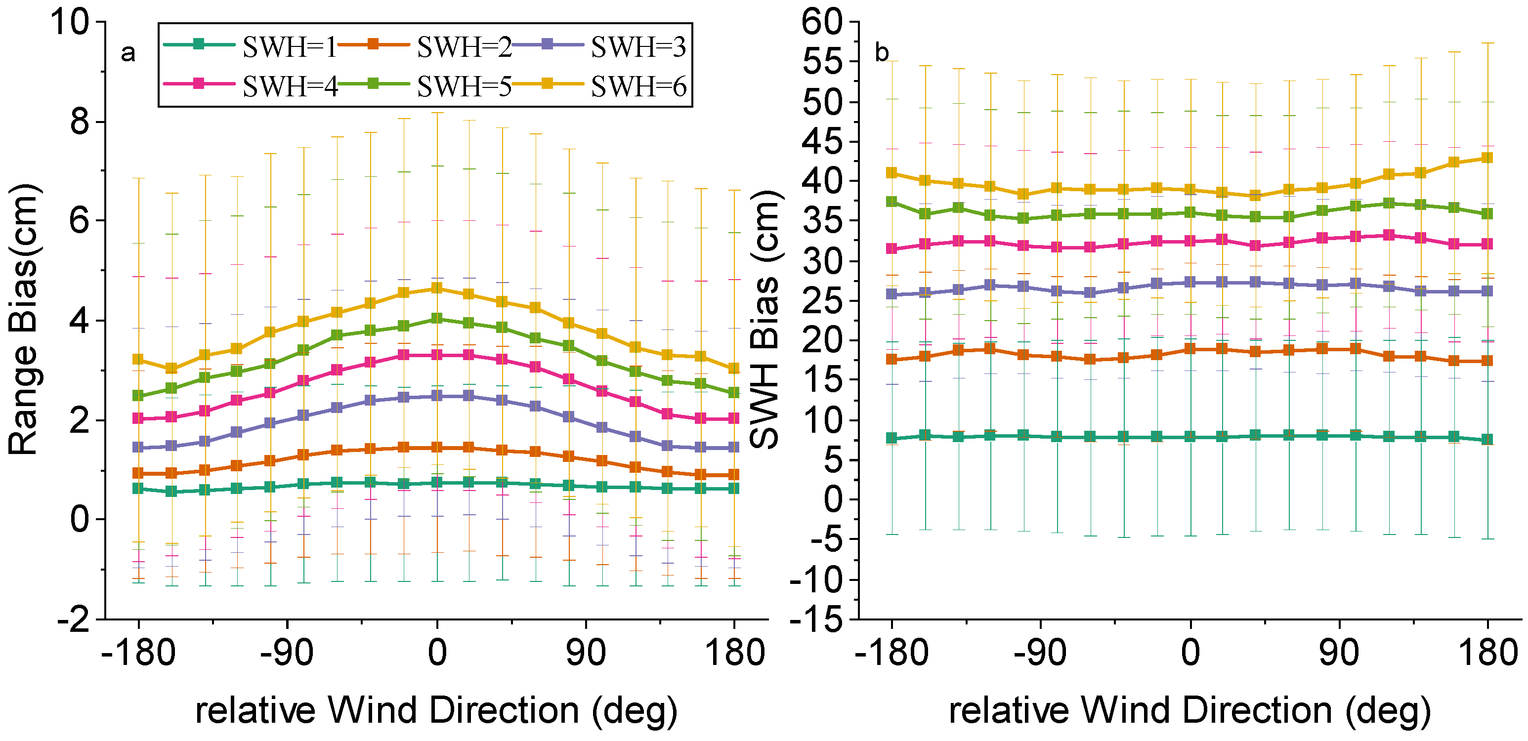
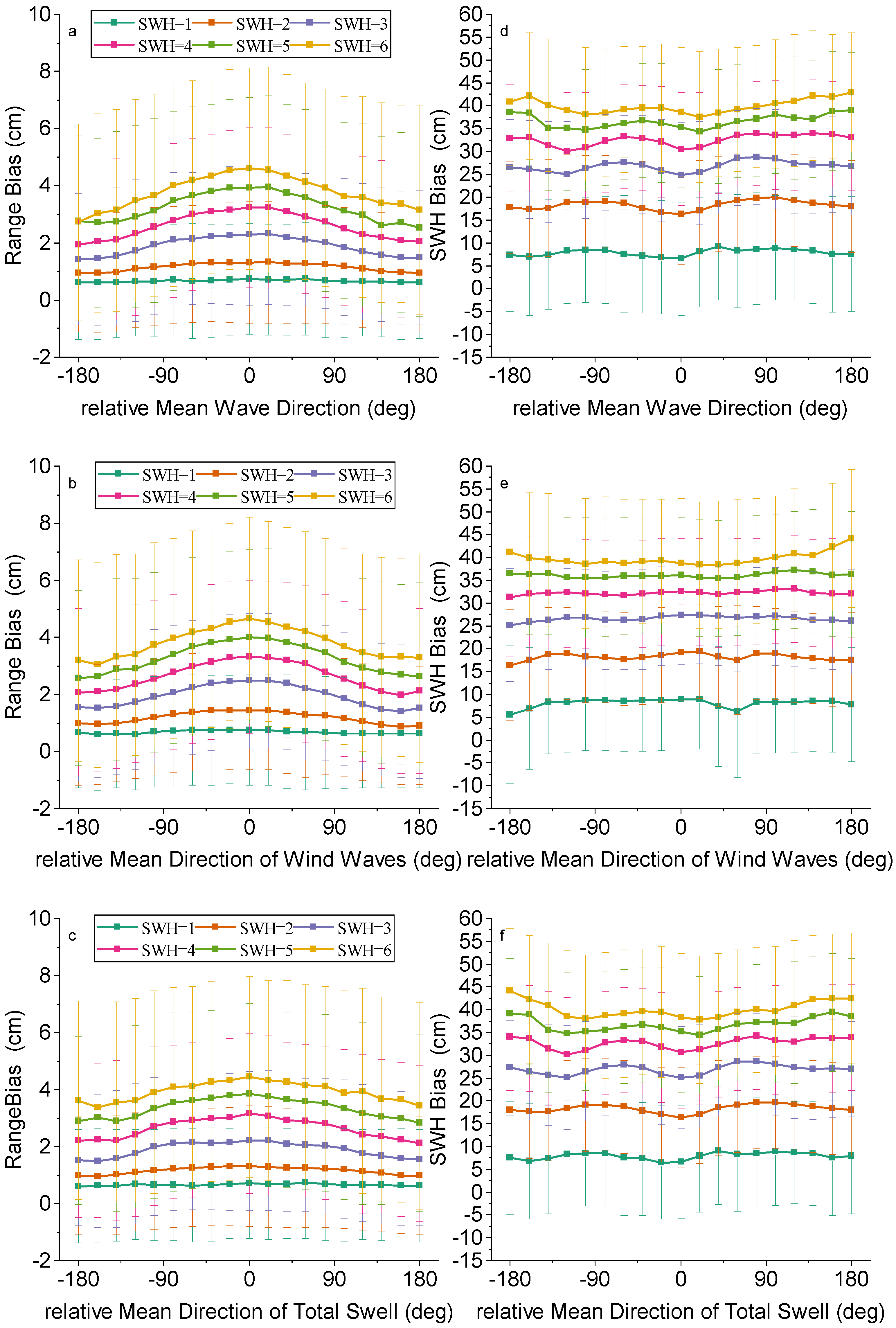
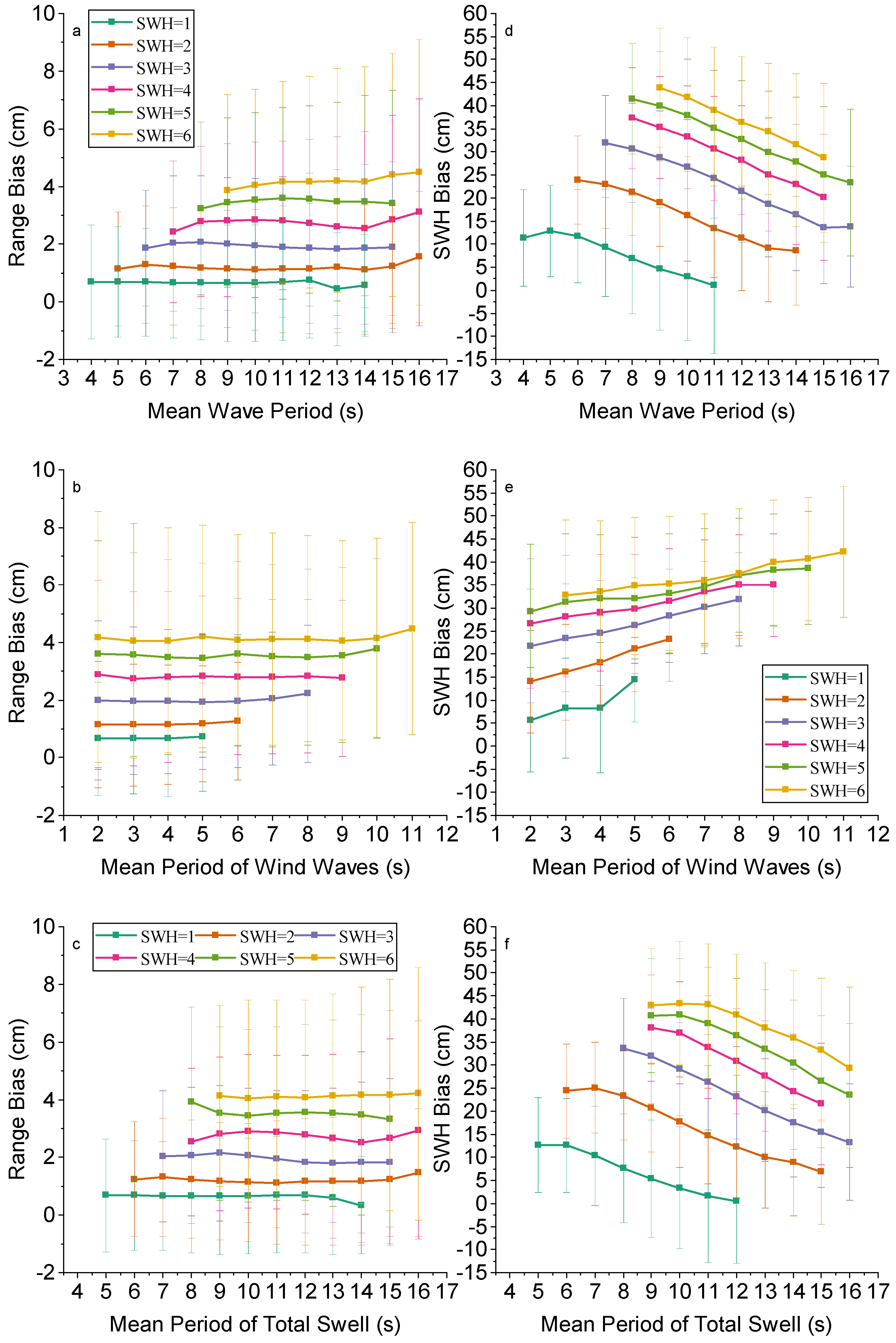
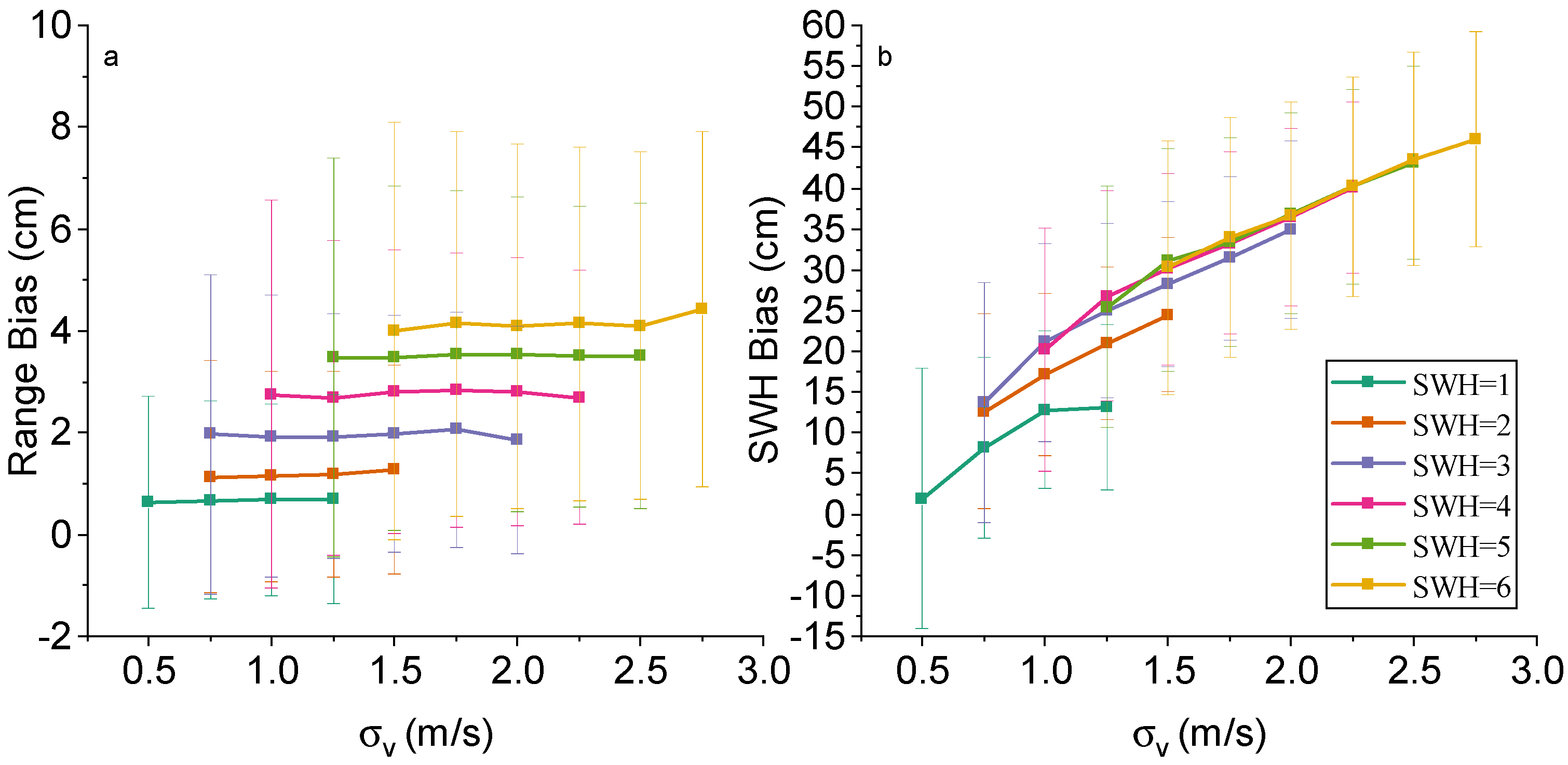
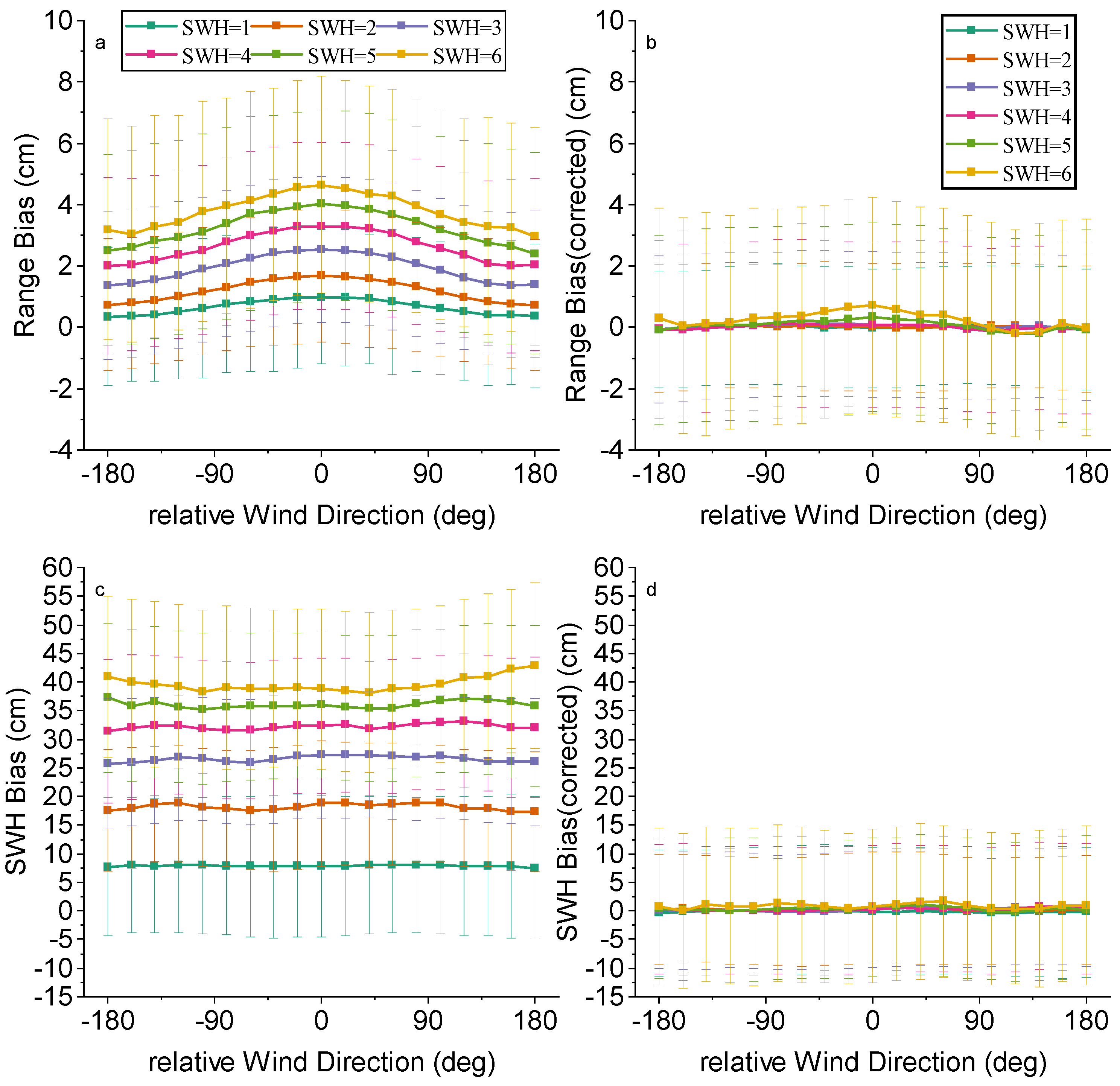
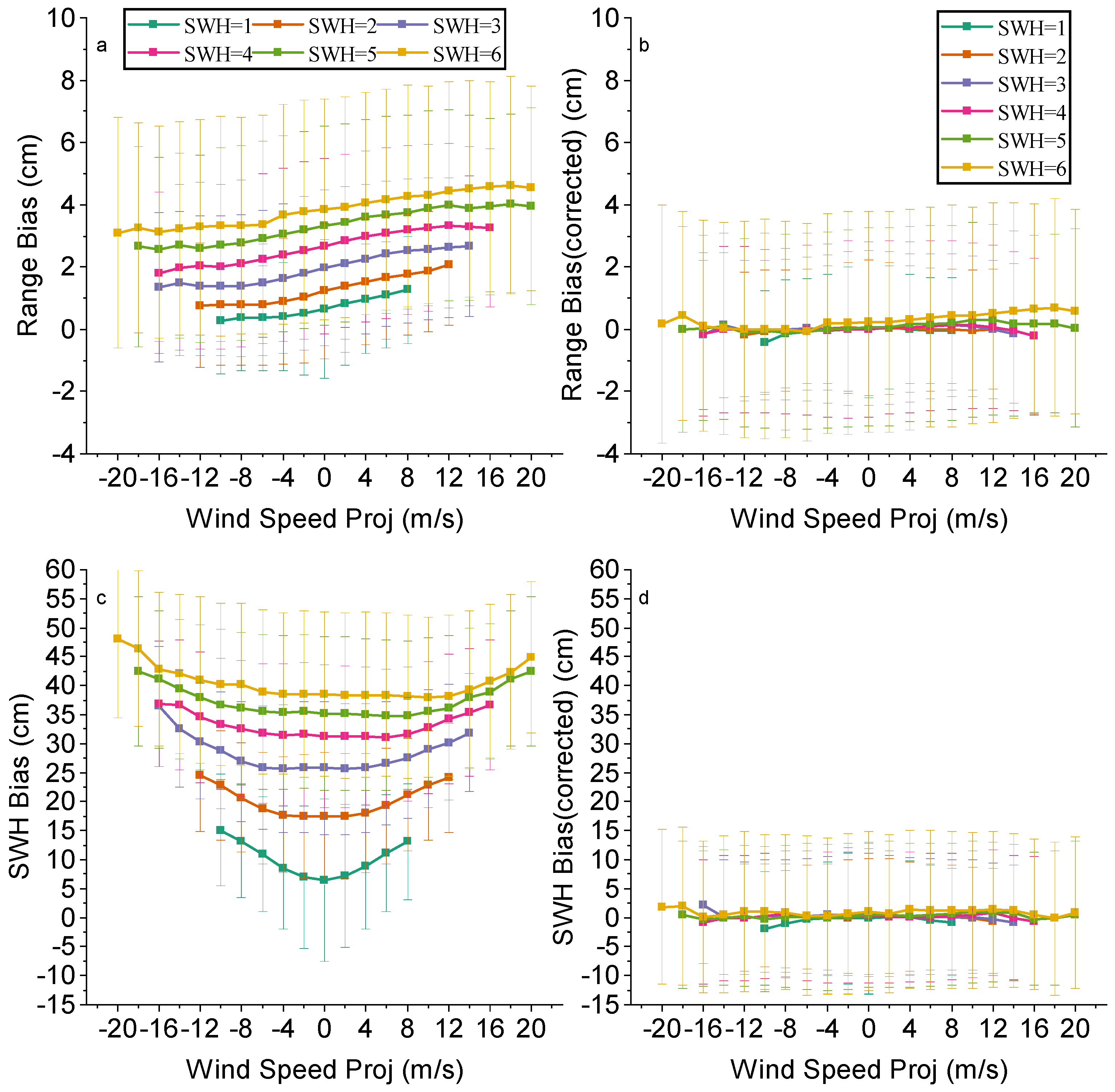
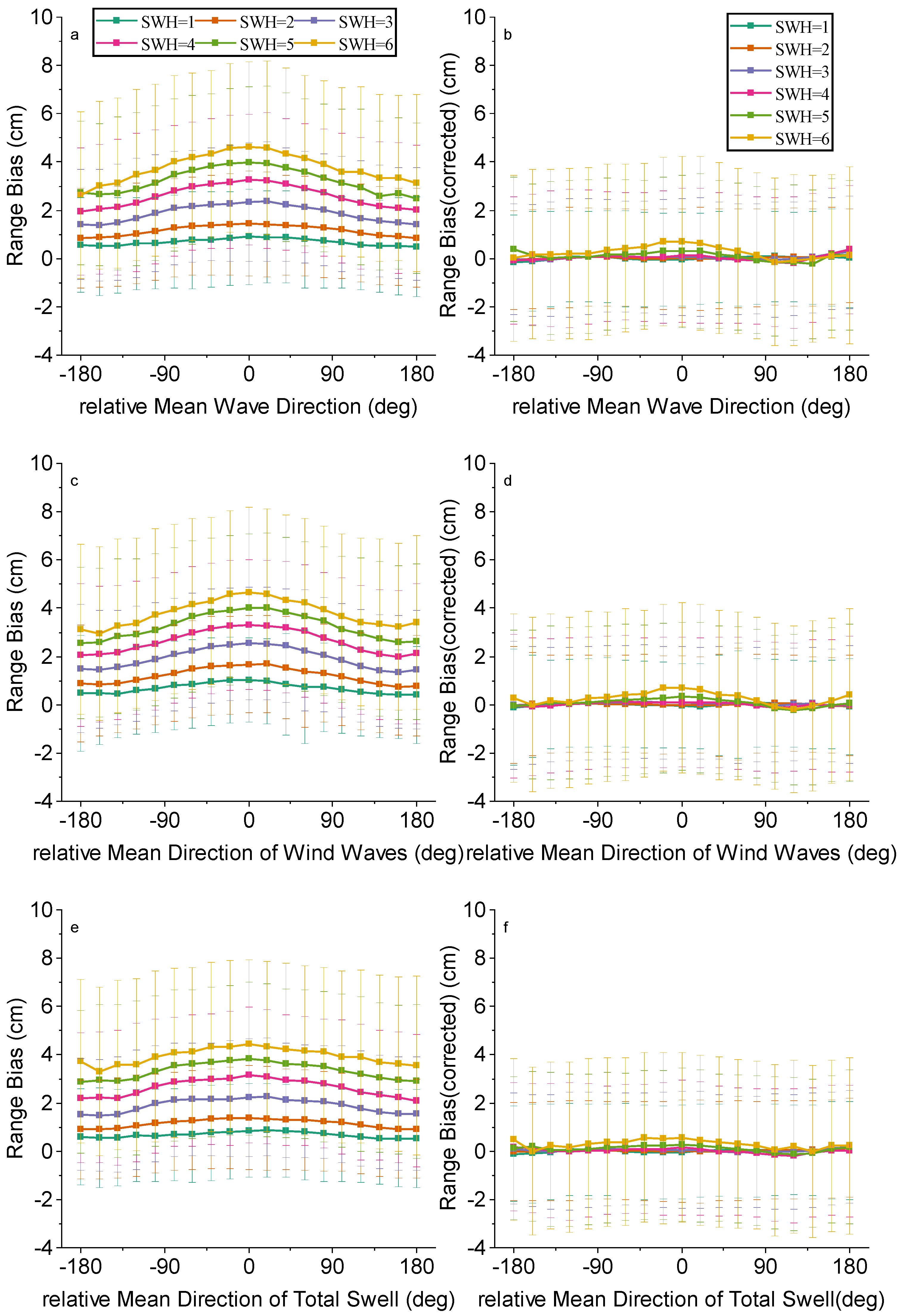
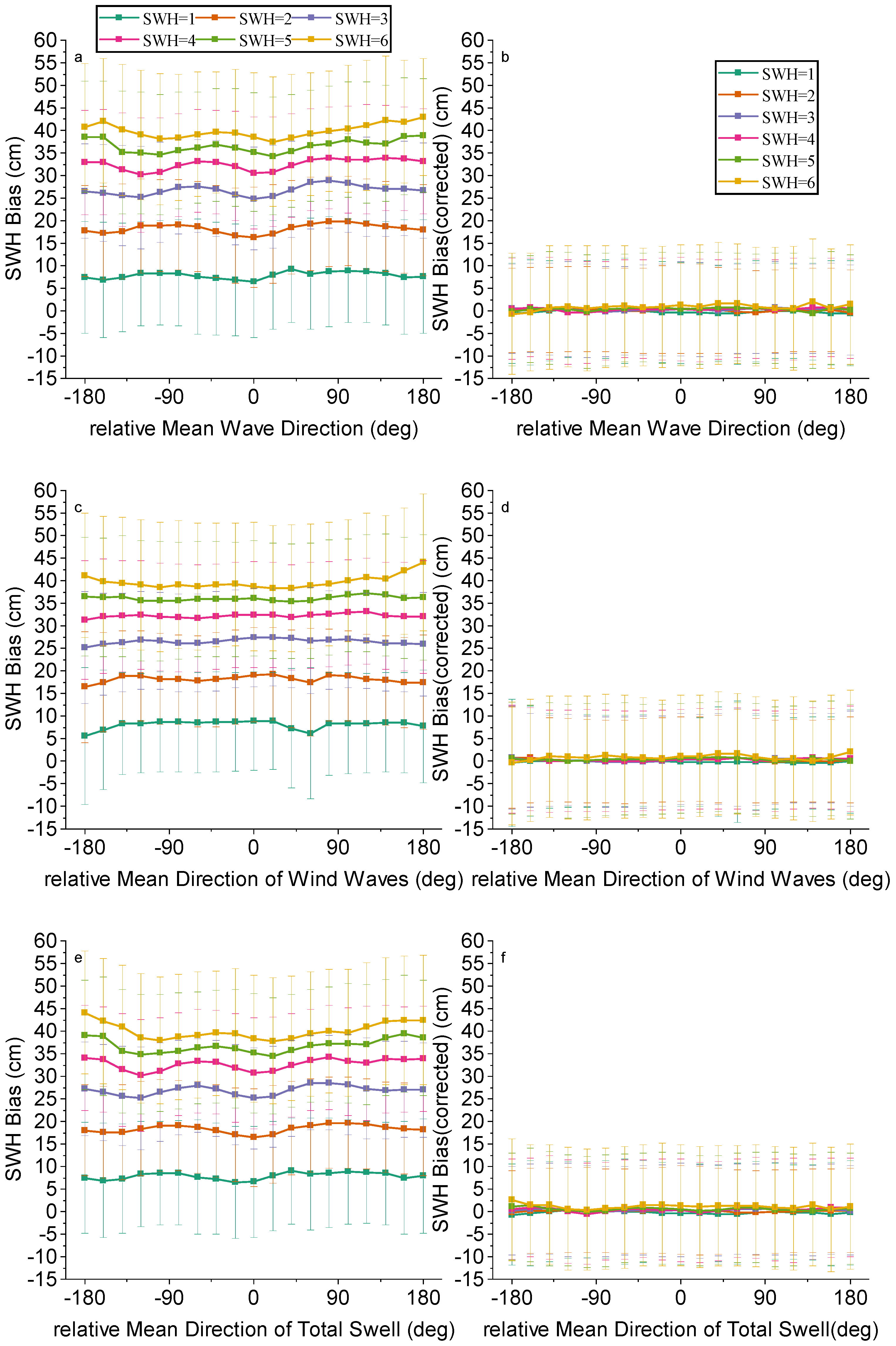
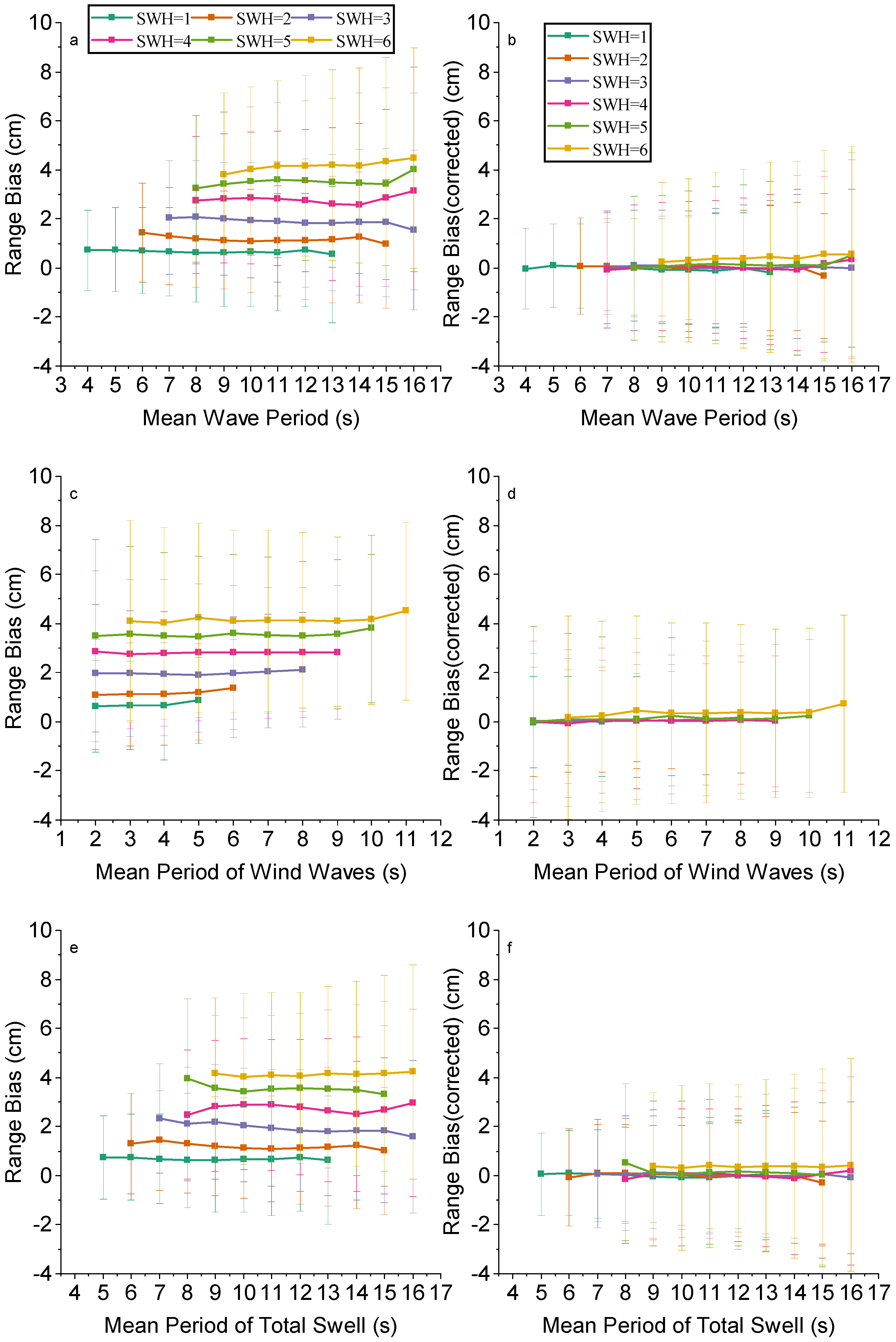
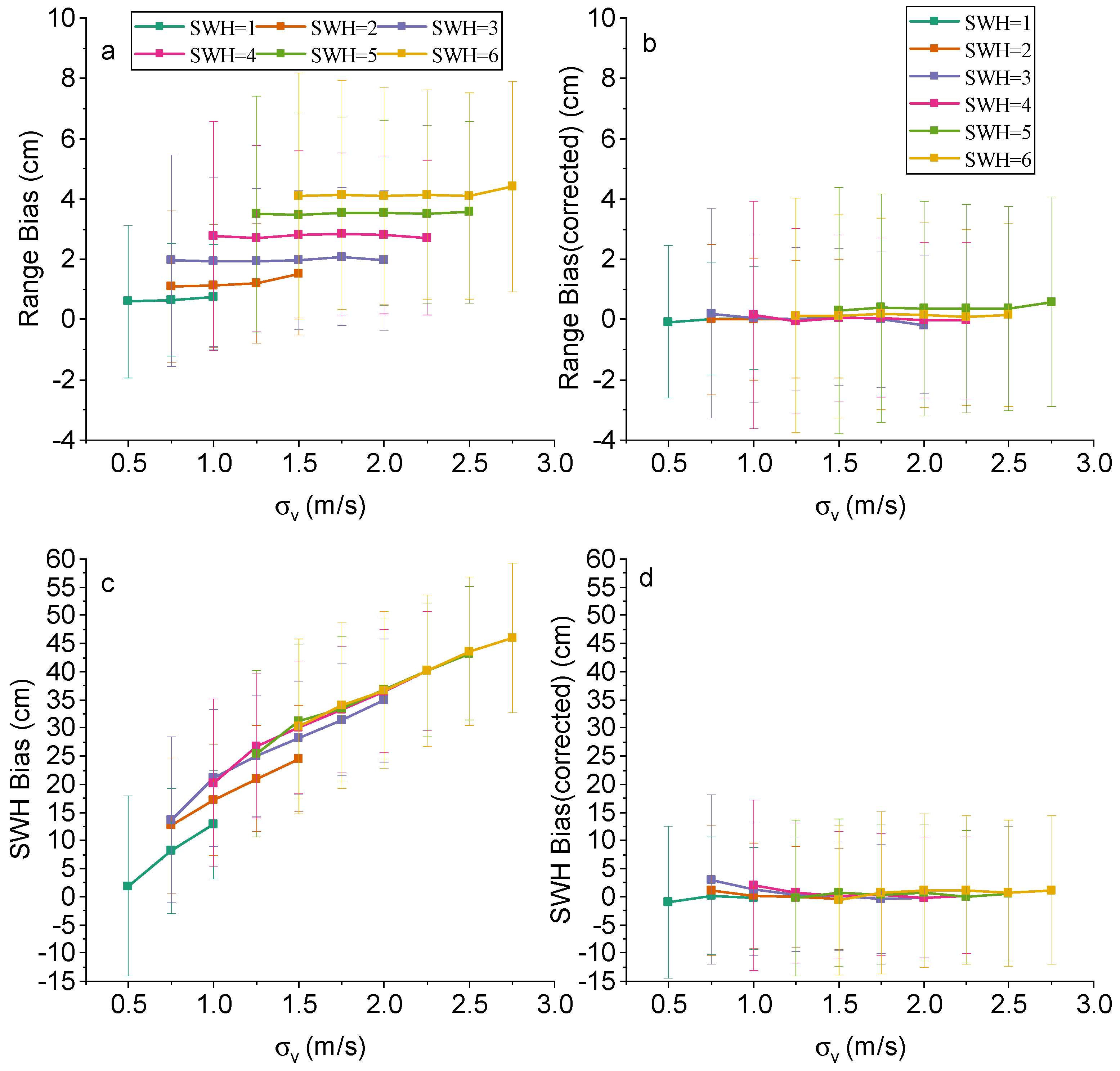
3.2. Impact of Ocean Waves on Range and SWH Biases Between HRM and LRM

Both practice and theory have shown that the wind and wave effects have a greater impact on HRM data than LRM. LRM values of range and SWH from modern retracking are the best representations there are of these quantities, and we are going to attempt to bring HRM data in line with them. This study analyzes the impact of ocean waves on SAR altimeter measurements through the analysis of real data from Sentinel-6. One year (from February 2023 to February 2024) of the Sentinel-6 LRM and HRM altimetry data are used. Biases of range and SWH between HRM and LRM are characterized concerning wave parameters extracted from ERA5 files.

Figure 4 shows the trend plot of range and SWH (obtained from Sentinel-6) bias as a function of SWH (obtained from ERA5), and it can be seen that the larger the SWH, the larger its bias. Figure 5 shows the SWH of LRM and HRM compared with the ERA5 model.

Figure 6 shows the Sentinel-6 range and SWH biases between HRM and LRM for different SWH values and relative wind directions. Figure 6a shows that the range bias increases with increasing SWH values, and the range bias with respect to the relative wind direction tends to be symmetric about 0°. As the value of SWH rises, the trend of range bias is similar across various relative wind directions; however, it generally increases. At SWH = 1 m, the range bias remains roughly in the range of 0.5 cm to 0.8 cm, whereas this range increases to 3 cm to 4.3 cm at SWH = 6 m. This indicates that the range bias increases accordingly with the rise in SWH. At different SWH levels, the maximum value of the range bias occurs at a relative wind direction of 0°. The range bias decreases as the absolute value of the relative wind direction increases, so the minimum value is at 180°. The relative wind direction affects the sea surface roughness and the strength of the radar echo signal. When the angle between the wind direction and the flight direction is small, the wind and waves scatter the radar signals more strongly, resulting in enhanced echo signals; thus affecting the range accuracy. When the wind direction is the same as the flight direction (i.e., the relative wind direction is 0°), the wind causes the amplitude of the waves (i.e., the sea surface undulation increases) to be the strongest, and this change manifests itself in the SAR echo signals as stronger fluctuations and greater sea surface undulation.

As shown in Figure 6b, the SWH bias is much higher compared to the ranging bias and has a flatter trend with relative wind direction. The SWH bias is almost a straight line at lower SWH values. At higher SWH values, there is a slight increase in SWH bias with increasing absolute values of relative wind direction. This indicates that the SWH bias is much less affected by the relative wind direction. SWH represents the significant wave heights across the wave field and is a statistical average that is influenced by a combination of factors. Relative wind direction may affect localized wave heights and patterns, but does not significantly change the statistical properties of the overall waves. Therefore, the sensitivity of SWH to changes in wind direction is relatively low.

Combining the results of the analyses in Figure 6, we can conclude that the relative wind direction has an influence on both range bias and SWH bias, but the degree of influence and the trend are different.

Figure 7 shows the impact of wind speed projection on range bias and SWH bias. It can be observed that the range bias and SWH bias vary significantly with the wind speed projection. This is related to the degree to which the relative wind direction’s influence on the range bias and SWH bias is significant. According to the formula of wind speed projection (Equation (4)), it can be analyzed that the effect of wind speed projection on the range bias is affected by both the relative wind direction and the magnitude of wind speed. However, for the SWH bias, the wind speed projection is mainly determined by the wind speed magnitude, and the relative wind direction has less influence, so it will show an approximate curve symmetric of about 0 m/s.

In addition, the range bias and SWH bias are in the range of 0.5–0.7 cm and 5–15 cm for SWH value of 1 m, but at SWH = 6 m, they are in the range of 3–4 cm and 39–47 cm. From SWH = 1 m to SWH = 6 m, the range bias increased by about 2.5 cm and the SWH bias increased by about 33 cm, which shows that as the SWH value increases, the range bias and SWH bias also increase.

As shown in Figure 7a, the range bias increases as the wind speed increases. They increase at approximately the same rate for SWH = 2 m to SWH = 6 m values. Wind speed projection directly affects sea surface roughness. Higher wind speeds increase the density of capillary and short gravity waves at the sea surface, leading to enhanced radar backscatter. Since SAR range measurements are based on the time of arrival of the radar pulse at the sea surface, anisotropy of the sea surface slope (especially along the direction of flight) can significantly change the rise time of the leading edge of the echo, thus affecting the range measurements.

Figure 7b demonstrates the trend of SWH bias with wind speed projection. It can be seen that the SWH bias increases as the wind speed magnitude increases. WSP indirectly affects wave energy and height by influencing wind wave generation and development. Higher wind speeds usually enhance the energy of wind waves, which in turn has some effect on SWH.

Figure 8 shows the impact of relative MWD, relative MDWW, and relative MDTS on range bias and SWH bias. The relative MWD, MDWW, and MDTS are obtained by the same calculation method as the relative wind direction. Also, the effects of these relative directions on the range bias and SWH bias follow the same trend as that of the relative wind direction on them. As shown in Figure 8a–c, the range bias is symmetric about 0° and the wave peaks at 0°, with a decreasing trend to both sides. As shown in Figure 8d–f, the effects of relative wave direction and relative swell direction on SWH bias show opposite trends, but both are symmetric about 0°, with a less pronounced and flatter trend to either side.

In addition, for range bias, the range of range bias affected by wind waves is roughly 3–4.3 cm, while the range affected by swell is only 3.8–4.2 cm at SWH = 6 m. For SWH bias, with the changes in these relative directions, the changes in all three biases are relatively similar, but it can also be seen that the amplitude of fluctuations under the influence of swell is much larger than that of wind waves. In summary, the range bias is primarily dominated by wind waves, while the SWH bias is mainly dominated by swells.

Relative wind wave direction and relative swell direction have a similar effect on range and SWH as relative wind direction, also by affecting echo strength. Higher effects of relative wind wave direction, especially when the wave propagation direction is close to the flight, result in increased range bias. The effect of swell is more specific and usually has less effect on range measurements due to its long period and smaller wave amplitude, but can still cause a bias. When the wave propagation direction coincides with the flight direction, the wave may appear higher, resulting in a large SWH. Conversely, when the surge propagation direction coincides with the measurement direction, the SWH may be underestimated because of the smaller amplitude of the surge wave.

Figure 9 shows the impact of MWP, MPWW, and MPTS on range bias and SWH bias. As shown in Figure 9a–c, for the range bias, the trend of the bias change is not obvious with the increase in the three wave periods. Especially for wind waves, it is almost a straight line. From Figure 9d–f they show that the trend of SWH bias is significantly more drastic than that of range bias. With the increase in the MWP and MPTS, the SWH bias shows a significant decreasing trend, and the range reaches 15 cm. Whereas with the increase in the MPWW, the SWH bias shows an increasing trend than that on range and increases from 32 cm to 42 cm at SWH = 6 m.

The wind wave period and swell wave period reflect the cyclic nature of ocean waves. Longer wave periods usually imply greater wave energy and more regular wave structure, which affect the reflection and scattering characteristics of radar signals. Wave periods have a more significant effect on SWH because they directly determine the height and energy of the waves, which directly affects SWH measurements. As the wind wave period increases, SWH typically increases because the wind wave energy is concentrated over a shorter range of wavelengths and wave heights are higher. Whereas, as the swell wave period increases, SWH typically decreases because the swell energy is dispersed over a longer range of wavelengths and wave heights are lower.

Range measurements are mainly dependent on the propagation time and reflection characteristics of the radar signal, and are less related to energy, so the wave period has almost no effect on range bias.

In summary, the impact of wave period on SWH bias is much larger than its effect on range bias, and their effects are the same for different SWH values.

Figure 10a illustrates the trend of range bias with the standard deviation of vertical velocity ${\sigma }_v$. With the increase in ${\sigma }_v$, the trend of range bias is the same for different SWH conditions with almost no fluctuation. The range bias increases only with the increase in SWH.

Figure 10b illustrates the trend of SWH bias with ${\sigma }_v$. As with the range bias, the SWH bias increases as the SWH value increases. However, unlike the range bias, the SWH bias varies more significantly with ${\sigma }_v$. It increases with the increase in ${\sigma }_v$, and the increase reaches about 20 cm at SWH = 6 m.

Since the vertical velocity standard deviation reflects the inhomogeneity of the vertical motion of the sea surface, it leads to the broadening of the radar echo waveform in the time domain. The larger the ${\sigma }_v$ is, the more significant the waveform broadening is (the standard deviation of the waveform increases). The SAR algorithm for retrieval directly estimates the SWH by measuring the slope of the waveform, so the ${\sigma }_v$ has a large effect on the SWH bias. And as mentioned before, range measurement is related to radar scattering and less related to sea surface undulation, so ${\sigma }_v$ has almost no effect on range bias.

Combining the analysis results in Figure 10, we can conclude that the vertical velocity standard deviation of the ocean wave has a significant effect on the SWH bias and almost no effect on the range bias.

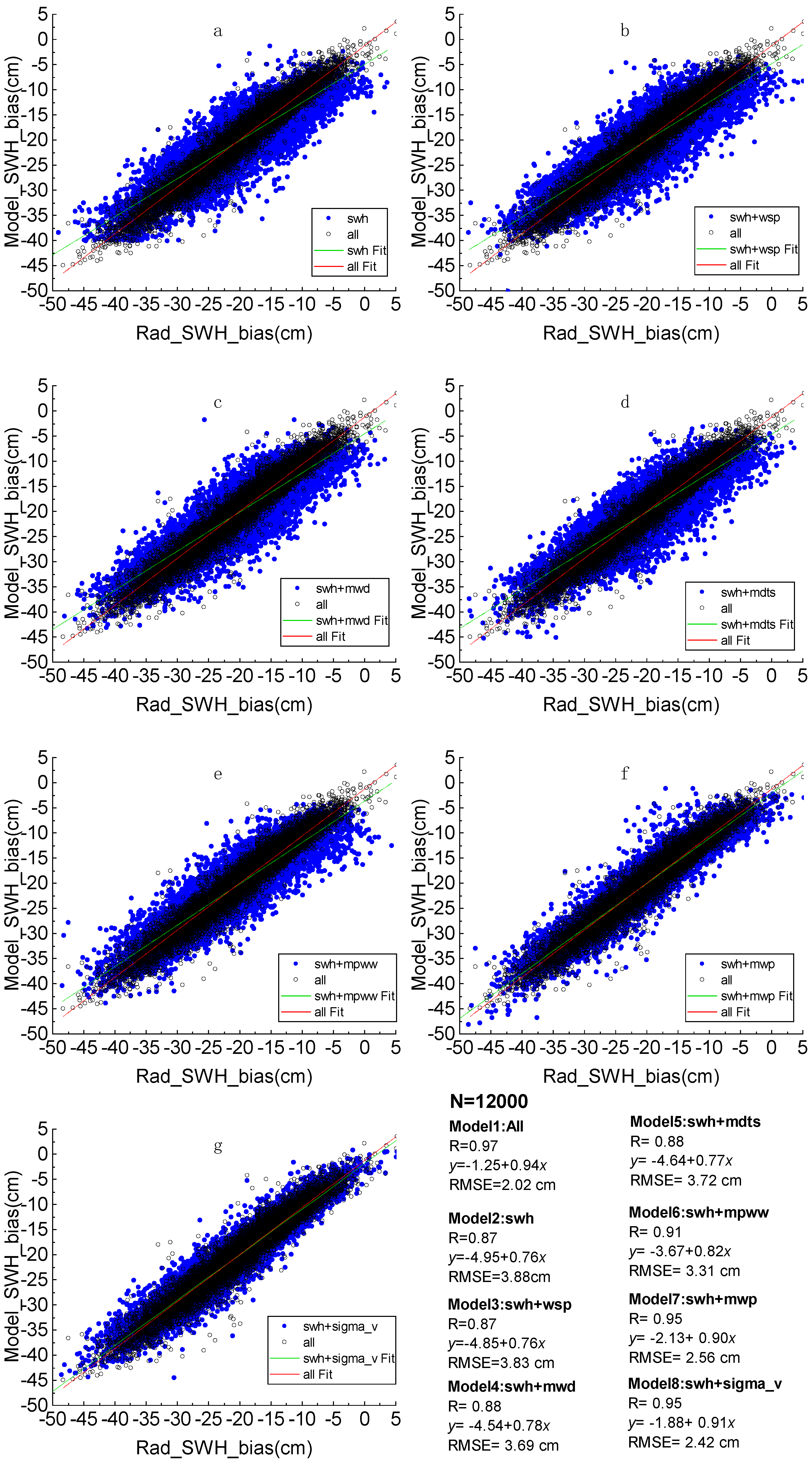
4. Range and SWH Corrections for the SAR Altimeters Using Neural Network

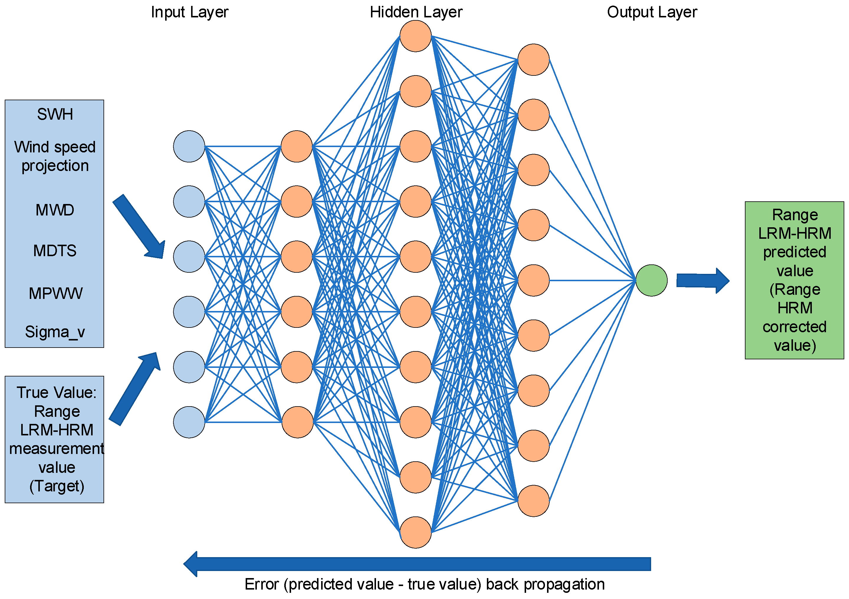
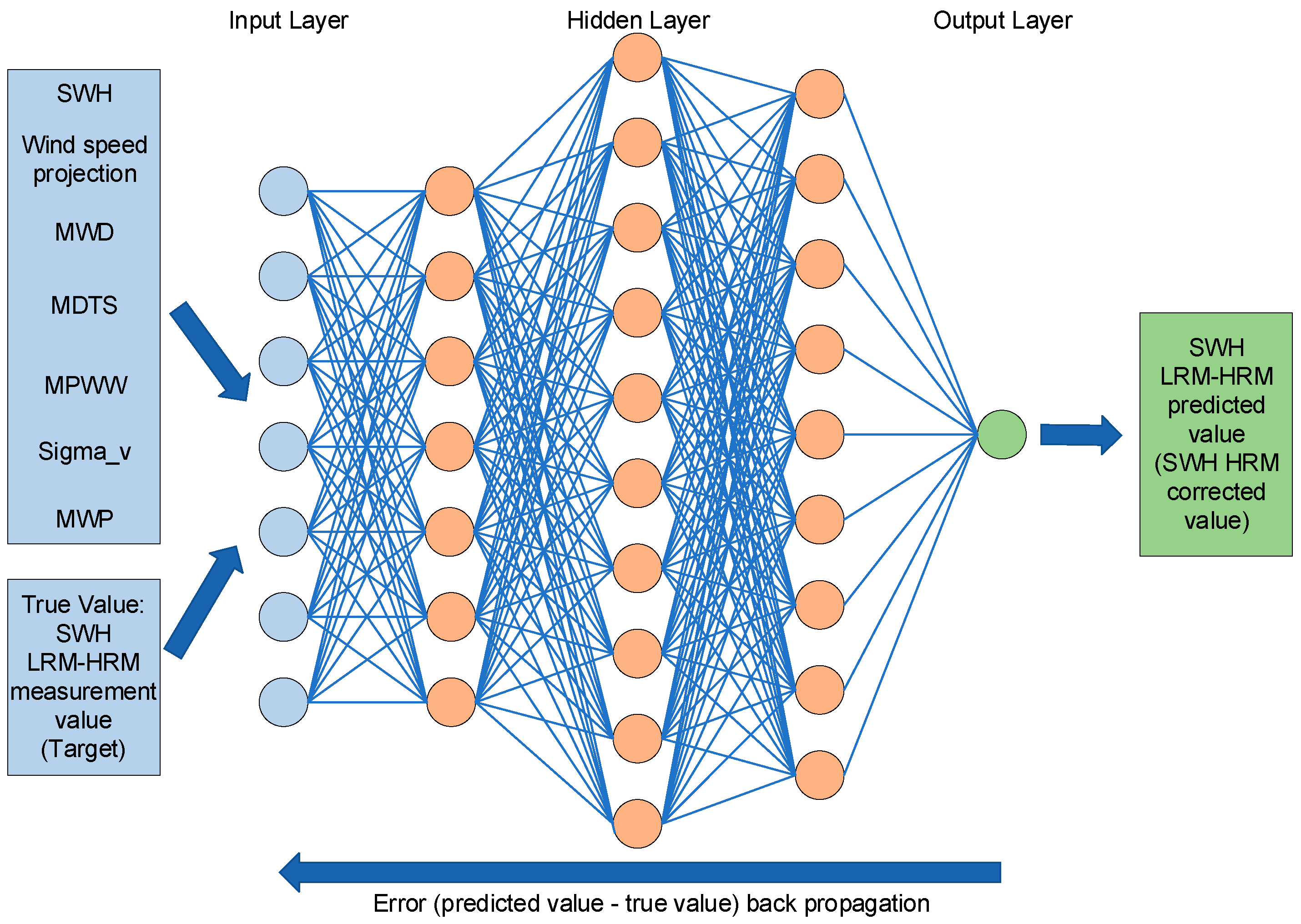
4.1. BP Neural Network Based Correction Method

This study constructs a BPNN (Back Propagation Neural Network) model to estimate the HRM range and SWH corrections for ocean wave impacts in SAR altimeter observations. The problem of obtaining corrected values for range bias and SWH bias through neural networks is essentially a regression problem; given feature values and target values, predictions are made utilizing regression fitting to find the relationship between the feature values and the target values to predict the output values for the new, unknown data points. For this problem, predictions are made by inputting the ocean wave parameter as the feature values, and the bias of the measured value, i.e., LRM minus HRM as the target value, finding the relationship, and outputting to obtain the correction value needed to reduce the impact of ocean wave movement on the HRM.

A BP neural network fundamentally establishes a mapping function from input to output, and mathematical theory indicates that a three-layer neural network may approximate any nonlinear function with arbitrary precision [53]. This renders it especially appropriate for addressing issues with intricate internal mechanisms; specifically, BP neural networks provide robust nonlinear mapping abilities. Furthermore, the BP neural network may autonomously derive the “reasonable rules” (the “reasonable rules” refer to the patterns and relationships that the BP neural network autonomously learns during training) between the inputs and outputs during training, while adaptively retaining the learned information within the network’s weights. The BP neural network possesses a significant capacity for self-learning and self-adaptation. The BP neural network has resilience, as localized or partial neuron damage does not significantly affect the overall training outcomes; thus, the system can continue to function correctly despite such impairments. For our current problem, i.e., bias correction of range and SWH measurements, using BP network training can obtain a better mapping, and at the same time, it is more fault-tolerant, and the network can also achieve better correction results by using other data later.

In response to the impact results analyzed previously, we use the neural network method to reduce the impact on the HRM, that is, to correct the HRM data. By inputting the influential wave parameters, we selected as feature values and LRM-HRM measurements as target values, and training the neural network, we obtain a network which can be applicable to universal data. At this point, the prediction data obtained from the output of the network is also the correction value of HRM, which is needed in the subsequent process. In other words, for the subsequent correction process, the correction value can be obtained by simply inputting the wave parameters into the trained network, and the correction value plus the HRM measurement is the corrected HRM data.

Figure 11 illustrates the network diagram for the range training model, whereas Figure 12 depicts the network diagram for the SWH training model. Based on the results of the above impact analysis, wind speed projection contains information about the relative wind direction, so we can select the wind speed projection as input for neural network. Furthermore, we find that the trends are approximately consistent in their relative direction, so here we can select relative MWD, and relative MDTS as a representation. Again, in the period section, it is enough to select only one parameter as a representative for the trend similarities, so we select MPWW as an input. At the same time, we can find that the impact of MPWW on SWH bias compared to range has a different trend from that of MWP and MPTS, so in the SWH model, we add MWP as an input again. And according to the previous analysis, ${\sigma }_v$ can also be found that it has an impact on both the range bias and SWH bias, so it can also be used as an input parameter. In conclusion, we select SWH, wind speed projection, relative MWD, relative MDTS, MPWW and ${\sigma }_v$ as inputs to the range neural network and SWH, wind speed projection, relative MWD, relative MDTS, MWP, MPWW and ${\sigma }_v$ as inputs to the SWH neural network. The networks have a single input layer, several hidden layers, and a single output layer. After extensive experimentation, three concealed layers were established, comprising 6 or 7 (6 for range model, 7 for SWH model) neurons in the first layer, 10 neurons in the second layer, and 9 neurons in the third layer. And we obtain range and SWH corrections at the output layer.

Prior to model training, we sampled the above one-year data by random sampling method and obtained a sample size of 60,000. The distribution of the training set, validation set, and test set during training is 70:15:15. Finally, we obtain the desired training model.

The data used for the next model comparison is a randomly selected 20% of the 60,000 data used to train the model.

Figure 13 shows a comparison of the performance of range bias and SWH bias when regression is fitted using both BPNN and linear fitting methods. Rad_Range_bias and Rad_SWH_bias on the x-axis represent the actual values of Range bias and SWH bias (i.e., radar measurements), and Predict_range_bias and Predict_SWH_bias on the y-axis represent the predicted values of Range bias and SWH bias. As illustrated in Figure 13a, the BPNN fitted curve aligns more closely with the y = x reference line (indicating the proximity between predicted and observed values) compared to the linear regression model, demonstrating its superior predictive performance. This is quantitatively supported by the range bias-corrected model results: the BPNN achieves an R-value of 0.93 with an RMSE is 0.30 cm while the linear model yields a lower R-value (0.87) and a higher RMSE (0.42 cm). Similarly, in the analysis of the correction model for SWH bias, the BPNN model achieved an R-value of 0.97 and an RMSE of 2.02 cm, whereas the linear fit model obtained an R-value of 0.94 and an RMSE of 2.63 cm. Figure 13b further corroborates these findings, as the fitted curve of the BPNN model is significantly closer to the y = x line compared to that of the linear fit model.

Figure 14 and Figure 15 are comparisons of the effects of the BPNN correction models with different input parameters. Figure 14 is a comparison of the correction models for range bias. The seven models are, Model 1 is the correction model with all input parameters used in this experiment (i.e., shown in Figure 11), which serves as a control group for the five plots; Model 2 is the correction model with only SWH as an input parameter; Model 3 is the correction model with SWH and WSP as input parameters; Model 4 is the correction model with SWH and relative MWD as input parameters; Model 5 is the correction model with SWH and MDTS as input parameters; Model 6 is the correction model with SWH and MPWW as input parameters; and Model 7 is the correction model with SWH and ${\sigma }_v$ as input parameters. Similarly, Figure 15 is a comparison of correction models for SWH bias, and according to Figure 12, there is one more SWH bias correction input parameter than range, so in addition to the seven models mentioned earlier, there is an additional Model 8 with SWH and MWP as input parameters.

As can be seen from Figure 14, using only SWH as an input parameter for the range correction model is that the correction effect is a little worse compared to the model used in this experiment, but its effect is also the most significant among the parameters. And by comparing the models, it can be found that excluding SWH as the biggest factor, the addition of WSP has the biggest effect on the effect of the correction model, which means that for range bias, the effects of SWH and WSP are dominant, followed by MWD.

And according to Figure 15, the effect of the model with only SWH input is still much different compared with the model used in the experiment, which indicates that for SWH bias, there are other factors besides SWH that have a greater influence on it. Comparison of these eight models reveals that the SWH + MWP and SWH + ${\sigma }_v$ models are closest to the model used in this experiment and have the best effect, which means that for SWH bias, the effects of SWH, MWP and ${\sigma }_v$ are dominant, followed by MPWW.

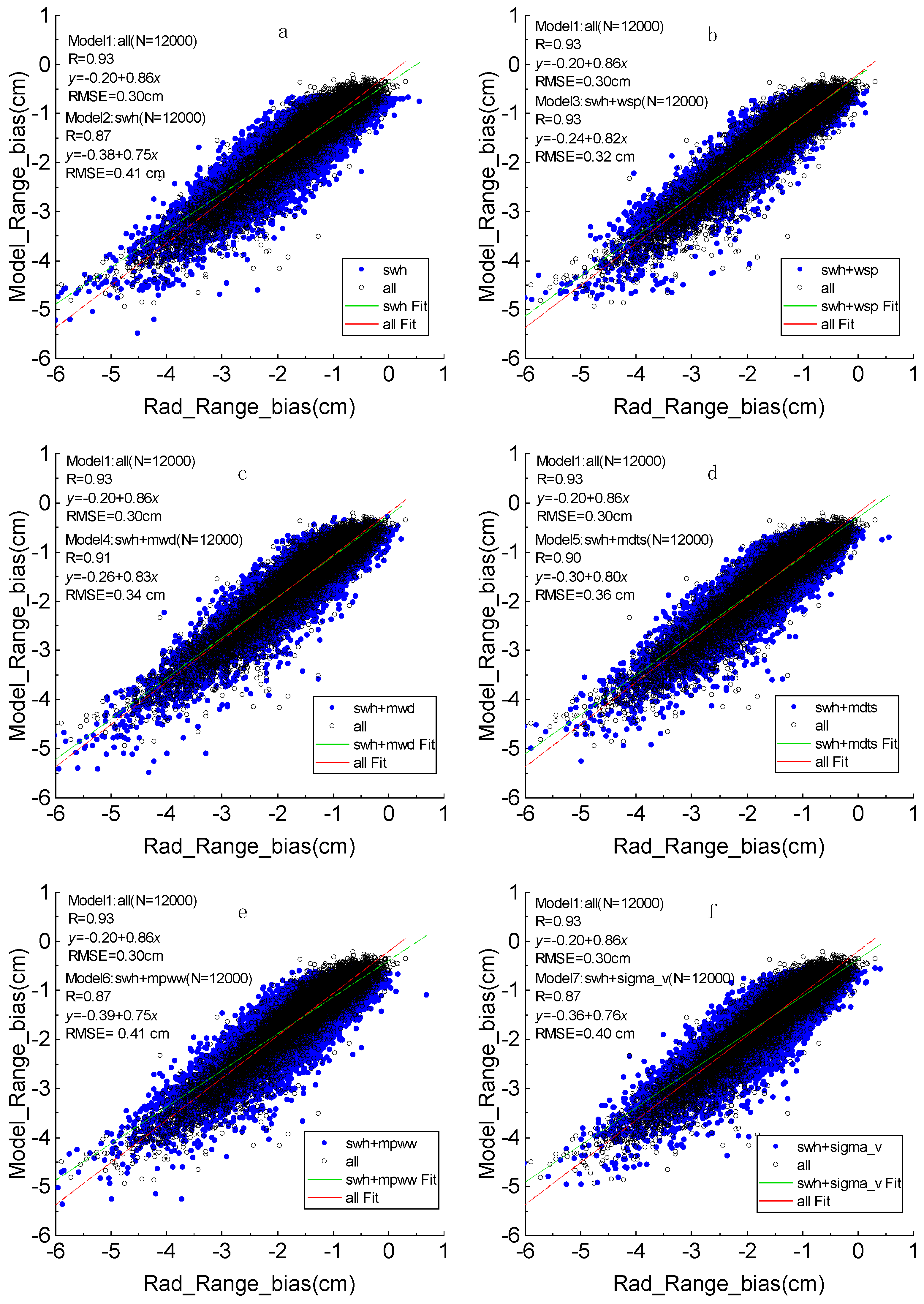
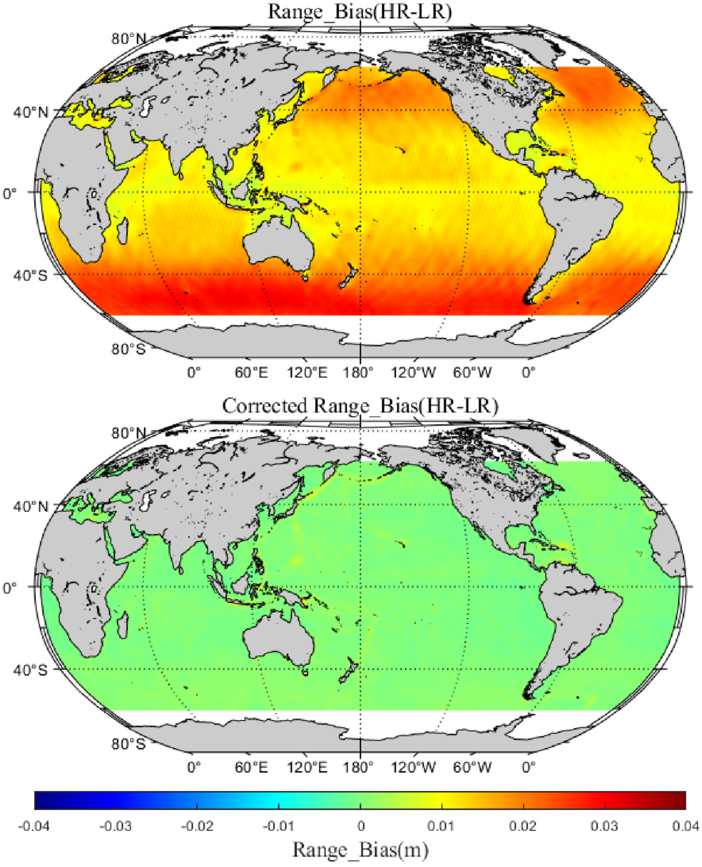
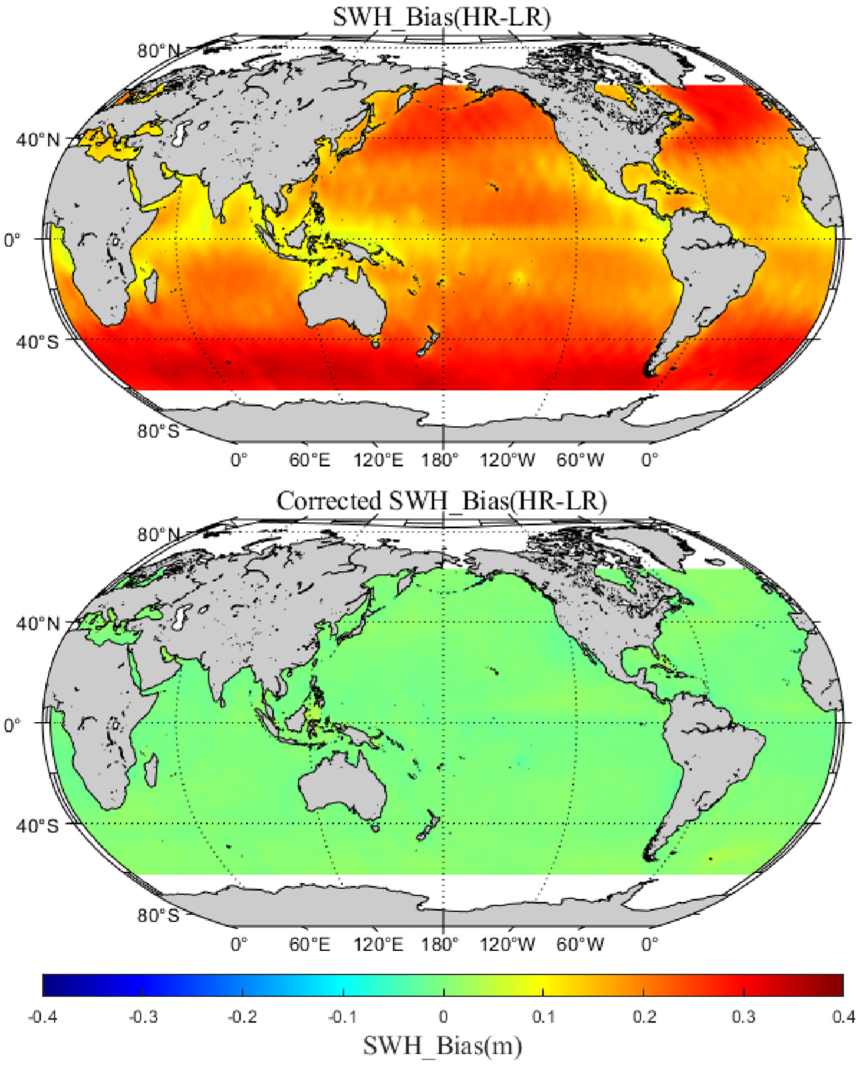
4.2. Comparison of the Range and SWH Biases Before and After Correction

By using the correction network trained in the previous step, we put wave parameters (input parameters in Figure 11 and Figure 12) into the corresponding correction network to obtain the range and SWH correction values. Then, the corrected range and SWH values in HRM can be obtained by adding the derived correction values to the previous HRM measurements.

Next, we repeat the previous impact analysis using the corrected range and SWH values to analyze the effect of different wave parameters on the corrected range bias and SWH bias in different SWH ranges and compare it with the impact analysis at uncorrected values.

In discussing the effects of the correction, we still use the one year of data mentioned in Section 2.1.

Figure 16a,b show the trend of range bias with relative wind direction before and after correction for different SWH ranges. It can be observed that under different SWH conditions, the magnitude of the variation in the corrected range bias with different wind directions is reduced compared to that before correction, especially at SWH = 1 m and SWH = 2 m, which indicates that the correction process effectively reduces the impact of waves on the range measurements. At the same time, the incremental magnitude of the range bias with SWH change is also greatly reduced after correction, showing the positive effect of the correction on improving the stability of the measurements.

Figure 16c,d show the trend of SWH bias with relative wind direction before and after correction in different SWH ranges. It can be seen that the correction achieves the same effect as that of the range bias correction, which reduces the influence of wind direction on the HRM measurement results and improves the stability and accuracy of the measurement.

Figure 17a,b show the trend of range bias with wind speed projection before and after correction. In Figure 17a, the range bias shows a increasing trend with increasing wind speed projection for all conditions from SWH = 1 m to SWH = 6 m, and range bias increases significantly with increasing SWH values. However, in Figure 17b, the change in range bias with wind speed projection is very small and almost constant for all SWH conditions, indicating that the impact of wind speed and SWH on range bias is significantly reduced after correction. Figure 17c,d show results for SWH bias. Again, it can be observed that the impact of wind speed on SWH bias is also significantly reduced after correction. SWH bias from varying with wind speed and SWH to almost a straight line. It means that the correction effect is also very effective.

Figure 18 illustrates the trend of range bias with relative MWD, relative MDWW and relative WDTS before and after correction. The left part of Figure 18 is before correction and the right part is after correction. Figure 18a,b are the comparison of range bias with relative MWD before and after correction, and we can find that the corrected range bias hardly varies with relative MWD. Figure 18c,d are the comparisons of range bias with relative MDWW before and after correction, and it can be observed that the variation in the corrected range bias tends to flatten out with relative MDWW for different SWH conditions, which indicates that the impact similarly reduced after correction. Figure 18e,f show the comparison of range bias with the relative mean direction of total swell before and after correction. Similarly, the corrected range bias is also almost a straight line around zero.

Figure 19 shows the trend of SWH bias with relative MWD, MDWW, and WDTS before and after correction. Like range bias, with the change in direction and SWH, the corrected SWH bias changes from a regular fluctuation before correction to a change with almost no fluctuation, which also proves that the correction effect is more obvious.

Figure 20 and Figure 21 show the trends of range bias and SWH bias with the MWP, MPWW, and MPTS before and after correction. As with the previous before and after correction figures where the bias changes with wave direction, the left side of Figure 20 and Figure 21 represents the bias before correction and the right side represents the bias after correction. It can be seen that with the change in wave period, there is a significant reduction in the bias after correction relative to before correction, which also indicates that the impact of the wave period is significantly reduced.

Figure 22 demonstrates the trend of range bias and SWH bias with vertical velocity standard deviation before and after correction. The upper panel of Figure 22 shows the comparison of the change in range bias with the STD of vertical velocity, and the lower panel for SWH bias. We can find that the impact of ${\sigma }_v$ on range bias and SWH bias is reduced obviously after correction, which demonstrates that the correction process effectively reduces the impact of the vertical motion of waves on the HRM values.

Figure 23 shows the global average distribution of range biases between HRM and LRM before and after correction. In the upper and lower plots, we can observe the impact of different geographic locations and the global effect of the correction. The before-correction bias is in the range of −0.04 m to 0.04 m, and the after-correction bias is concentrated near 0 m, i.e., a large area that shows a green color. This indicates that the correction effect is significant and no obvious range inconsistencies exist between HRM and LRM, which may provide better measurements for global and regional sea level rise studies.

Figure 24 shows the results for the SWH biases. It can also be seen that there is a good correction effect by comparing up and down. From the range of −0.4 m to 0.4 m before correction to the concentration near 0 m after correction, it also shows green color in a large area, indicating that the correction effect on SWH is also significant. The SWH biases may induce biases in the sea level measurements through sea state bias corrections. Therefore, the corrected SWH measurements can be used to provide more accurate sea level measurements.

As shown in Figure 24 we can see that there is a relationship between SWH bias and latitude. The SWH is relatively high in high-altitude areas; therefore the range and SWH biases are relatively high. In addition, through Figure 8 and Figure 10 we can see that the swell direction and the vertical velocity have a significant effect on the measurement of the SAR altimeter, and the waves at high latitudes usually have longer wavelengths and higher vertical velocities, which may be one of the reasons for the larger deviation of SWH at high latitudes.

5. Accuracy Assessment of the Corrected SSH and SWH Measurements

As shown in Section 4.2, the application of range and SWH corrections significantly reduces the biases between the HRM and LRM range and SWH measurements. It is also necessary to evaluate whether the application of range and SWH corrections changes the accuracies of the SSH and SWH measurements. In this study, we assess the accuracies of the corrected SSH and SWH measurements by using crossover analysis and comparing them against the NDBC buoy data, respectively.

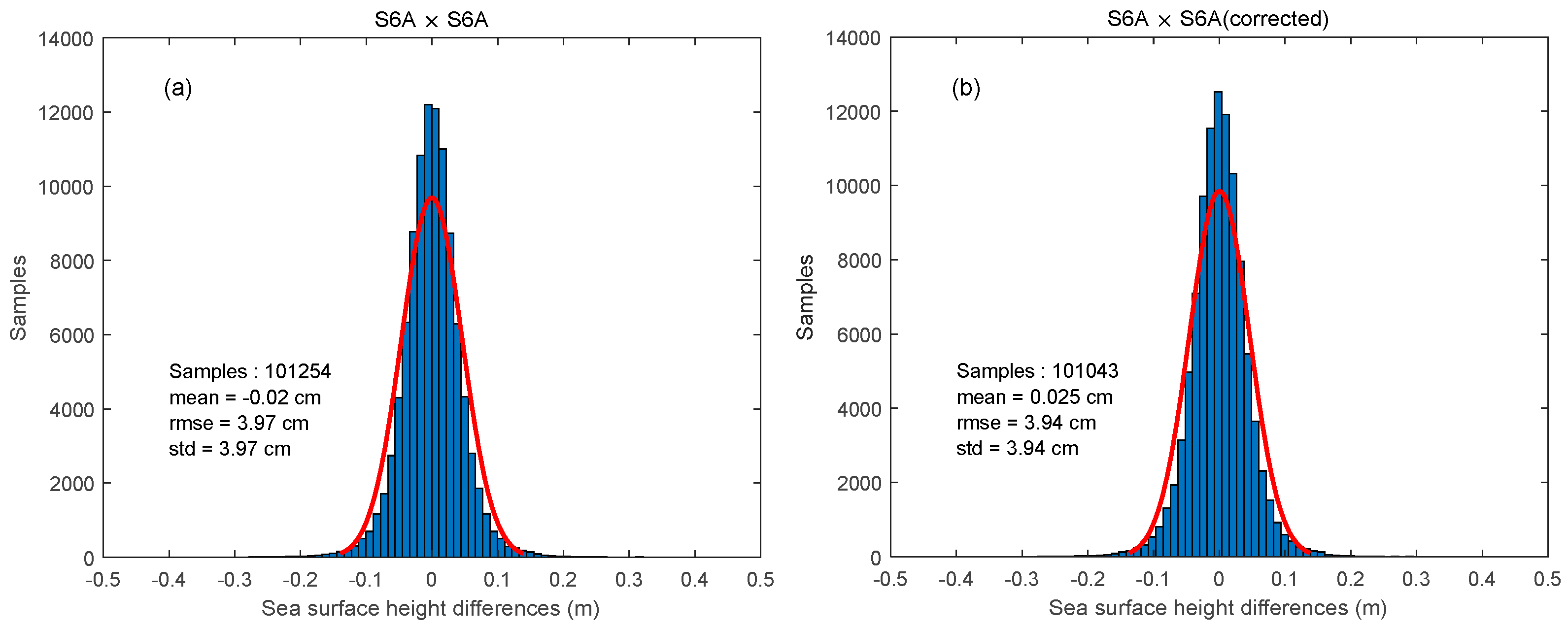
5.1. Assessment of SSH Using Crossover Analysis

The global sea surface height (SSH) crossover analysis is a prevalent technique for evaluating the accuracy of SSH values derived from altimetry data. The mono-mission crossover study evaluates the consistency between ascending and descending satellite orbits. In this study, we use the crossover analysis method [52] to assess the accuracy of the SSH measurements prior to and subsequent to correction. The SSH obtained from the altimeter can be represented as:

$$SSH=H-(R+\Delta R_{corr})$$

(7)

$$\Delta R_{corr}=\Delta R_{dry}+\Delta R_{wet}+\Delta R_{iono}+\Delta R_{ssb}+\Delta R_{ocean}+\Delta R_{solid}+\Delta R_{pole}+\Delta R_{DAC}$$

(8)

where $H$ is the satellite altitude above the reference ellipsoid, and $R$ is the altimeter range, $\Delta R_{dry}$ is the dry tropospheric correction, $\Delta R_{wet}$ is the wet tropospheric correction, $\Delta R_{iono}$ is the ionospheric correction, $\Delta R_{ssb}$ is the sea state bias correction, $\Delta R_{ocean}$ is the geocentric ocean tide, $\Delta R_{solid}$ is the solid earth tide, $\Delta R_{pole}$ is the polar tide and $\Delta R_{DAC}$ is the dynamic atmospheric correction. The range corrections we use are those provided in the altimetry products. The SSH measurements are calculated by applying the radiometer wet tropospheric correction and the filtered dual-frequency ionospheric correction.

The mean and STD of the SSH crossover differences are computed. To mitigate the effect of sea ice, only data within 50° of the Equator were used. The duration for the crossover variations in this study was set to 3 days. Figure 25 shows the histogram of the distribution of the SSH crossover differences before and after correction, respectively. The mean and STD of the HRM SSH differences at crossovers have no significant changes before (mean: −0.02 cm, STD: 3.97 cm) and after (mean: −0.025 cm, STD: 3.94 cm) correction. Therefore, the application of range correction does not change the accuracy of the HRM SSH measurements.

The crossover analysis is only a relative accuracy evaluation method, and it cannot provide accurate reference sea surface height measurements. The directional effect in the new correction may not be detected using this method. In addition, the range used in this study are not corrected for SSB. The SSB corrections used to calculate the SSH measurements are derived from the Sentinel-6 L2 altimetry data and it may affect the results. In the future, we will further develop an empirical method to correct the range or SSH including the classical SSB (tilt and hydrodynamic modulations) and the new effects (dynamics or ocean waves).

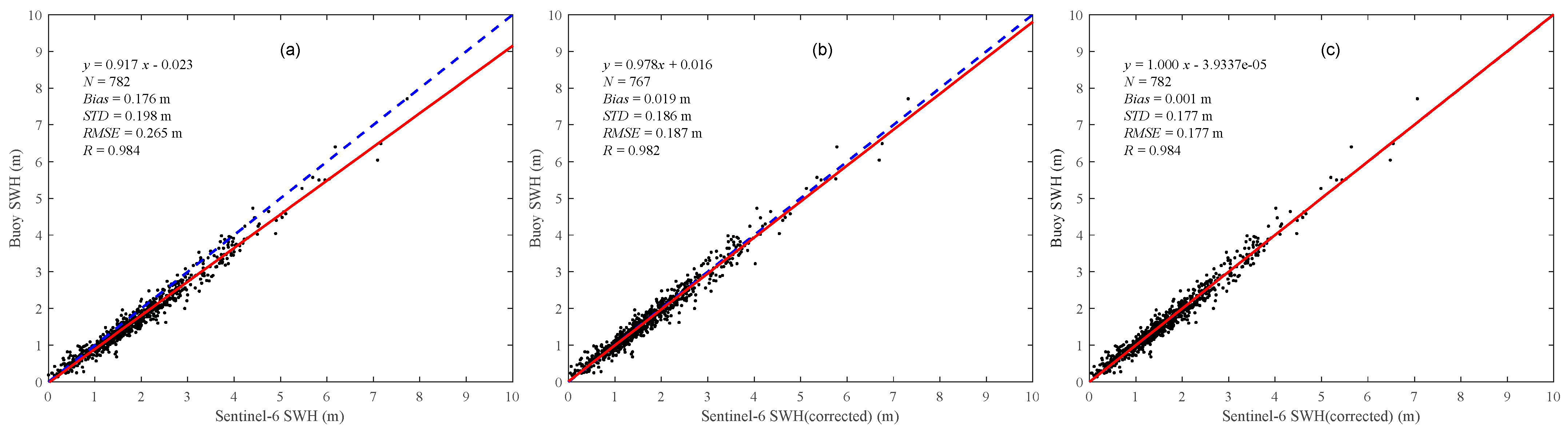
5.2. Assessment of SWH Using NDBC Buoys Data

The SWH measurements obtained from altimeters are usually validated by comparing them with NDBC data. The first step was to collate the altimeter and NDBC buoy data. We select altimeter data that are within 50 km of the buoy position and calculated the average of these values to represent the satellite altimeter data. Quality control was carried out before taking the average value. NDBC SWH measurements are linearly interpolated to correspond with the timing of the altimeter observations. A single collocation is formed from this interpolated NDBC data and the averaged altimeter measurement. Only those collocations with a time difference in under 0.5 h are utilized.

Figure 26a,b shows the scatterplots of Sentinel-6 HRM SWH measurements against the NDBC buoys before and after correction, respectively. The Sentinel-6 HRM SWH measurements after correction have an RMSE of 0.187 m with a bias of 0.019 m, which is significantly lower than the results before correction (RMSE: 0.265 m, bias: 0.176 m). Therefore, the application of SWH correction significantly improves the accuracy of the HRM SWH measurements.

Figure 26c shows that a simple linear adjustment of original SWH (SWH_corrected = 0.917×SWH_HRM − 0.023) would give almost the same overall improvement as BPNN. The analysis results in Section 3.2 show that the SWH bias significantly depends on the value of SWH and minorly on other impact factors. Therefore, a simple method to directly correct the SWH using only SWH is feasible. However, the SWH biases are also impacted by some parameters such as wind speed and vertical velocity. Therefore, we think it is more reliable to correct the HRM SWH values using more parameters such as SWH, wind speed and vertical velocity. In addition, as shown in Figure 3, the spatial coverage of the NDBC buoys is poor and irregular and the NDBC buoys SWH measurements are not able to be used to evaluate the SWH measurements over the open ocean.

6. Summary and Conclusions

The SAR altimeter has demonstrated better precision and along-track resolution compared to the conventional pulse-limited altimeter, facilitating extensive research into the observation of small-scale ocean phenomena. However, the SAR altimeter measurements exhibit sensitivity to ocean waves, resulting in inaccuracies in the estimates. In this study, we focus on analyzing the impact of ocean waves on the SAR altimeter measurements using Sentinel-6 real HRM and LRM data analysis and reducing the inconsistencies between the HRM and LRM range and SWH measurements.

The Sentinel-6 altimetry data and ERA5 re-analysis data are used to characterize the impact of ocean waves on the SAR altimeter measurements. The analysis is based on range and SWH differences between HRM and LRM concerning different wave parameters derived from model data. Results show that each wave parameter has different trends and degrees of impact on the range bias and SWH bias. The HRM range and SWH measurements are significantly impacted by SWH, vertical velocity and wind speed.

After analyzing the impact of different wave parameters on the range bias and SWH bias, we use the BP neural network training to obtain a correction network. Using this network, we obtain the correction values of the HRM range and SWH and then analyze the bias of the corrected HRM range and SWH values and compare them with the HRM values before correction. Results show that the application of these corrections highly reduces the biases between the HRM and LRM range and SWH measurements.

Finally, we assess the accuracies of the corrected SSH and SWH measurements by using crossover analysis and comparing them against the NDBC buoy data, respectively. Results show that the application of range and SWH corrections do not change the accuracy of the HRM SSH measurements, whereas they significantly improve the accuracy of the HRM SWH measurements. The STD of the HRM SSH differences at crossovers has no significant changes before (3.97 cm) and after (3.94 cm) correction. Compared to the NDBC measurements, the corrected HRM SWH measurements have an RMSE of 0.187 m, significantly better than that with no correction (0.265 m). The range and wave height correction method proposed in this study may provide a high-precision, unbiased continuation of the historical timeseries of sea level and SWH.

References

1. Doglioni, F.; Ricker, R.; Rabe, B.; Barth, A.; Troupin, C.; Kanzow, T. Sea surface height anomaly and geostrophic current velocity from altimetry measurements over the Arctic Ocean (2011–2020). Earth Syst. Sci. Data 2022, 15, 225–263. [Google Scholar] [CrossRef]
2. Cao, Y.; Dong, C.; Qiu, Z.; Bethel, B.J.; Shi, H.; Lü, H.; Cheng, Y. Corrections of mesoscale eddies and kuroshio extension surface velocities derived from satellite altimeters. Remote Sens. 2023, 15, 184. [Google Scholar] [CrossRef]
3. Morrow, R.; Traon, P.Y.L. Recent advances in observing mesoscale ocean dynamics with satellite altimetry. Adv. Space Res. 2012, 50, 1062–1076. [Google Scholar] [CrossRef]
4. Wang, G.; Su, J.; Chu, P.C. Mesoscale eddies in the South China Sea observed with altimeter data. Geophys. Res. Lett. 2003, 30, OCE 6-1. [Google Scholar] [CrossRef]
5. Ablain, M.; Meyssignac, B.; Zawadzki, L.; Jugier, R.; Picot, N. Uncertainty in satellite estimates of global mean sea-level changes, trend and acceleration. Earth Syst. Sci. Data 2019, 11, 1189–1202. [Google Scholar] [CrossRef]
6. Chen, X.; Zhang, X.; Church, J.A.; Watson, C.S.; King, M.A.; Monselesan, D.; Legresy, B.; Harig, C. The increasing rate of global mean sea-level rise during 1993–2014. Nat. Clim. Change 2017, 7, 492–495. [Google Scholar] [CrossRef]
7. Zhu, C.; Guo, J.; Yuan, J.; Li, Z.; Liu, X.; Gao, J. SDUST2021GRA: Global marine gravity anomaly model recovered from Ka-band and Ku-band satellite altimeter data. Earth Syst. Sci. Data 2022, 14, 4589–4606. [Google Scholar] [CrossRef]
8. Sandwell, D.T.; Müller, R.D.; Smith, W.H.F.; Garcia, E.; Francis, R. New global marine gravity model from CryoSat-2 and Jason-1 reveals buried tectonic structure. Science 2014, 346, 65–67. [Google Scholar] [CrossRef]
9. Li, Z.; Guo, J.; Ji, B.; Wan, X.; Zhang, S. A review of marine gravity field recovery from satellite altimetry. Remote Sens. 2022, 14, 4790. [Google Scholar] [CrossRef]
10. Smith, W.H.F.; Sandwell, D.T. Global sea floor topography from satellite altimetry and ship depth soundings. Science 1997, 277, 1956–1962. [Google Scholar] [CrossRef]
11. Fan, D.; Li, S.; Li, X.; Yang, J.; Wan, X. Seafloor topography estimation from gravity anomaly and vertical gravity gradient using nonlinear iterative least square method. Remote Sens. 2021, 13, 64. [Google Scholar] [CrossRef]
12. Hart-Davis, M.G.; Piccioni, G.; Dettmering, D.; Schwatke, C.; Passaro, M.; Seitz, F. EOT20: A global ocean tide model from multi-mission satellite altimetry. Earth Syst. Sci. Data 2021, 13, 3869–3884. [Google Scholar] [CrossRef]
13. Lyard, F.H.; Allain, D.J.; Cancet, M.; Carrère, L.; Picot, N. FES2014 global ocean tide atlas: Design and performance. Ocean Sci. 2021, 17, 615–649. [Google Scholar] [CrossRef]
14. Slater, T.; Shepherd, A.; McMillan, M.; Muir, A.; Gilbert, L.; Hogg, A.E.; Konrad, H.; Parrinello, T. A new digital elevation model of Antarctica derived from CryoSat-2 altimetry. Cryosphere Discuss. 2018, 12, 1551–1562. [Google Scholar] [CrossRef]
15. Helm, V.; Humbert, A.; Miller, H. Elevation and elevation change of Greenland and Antarctica derived from CryoSat-2. Cryosphere Discuss. 2014, 8, 1539–1559. [Google Scholar] [CrossRef]
16. Laxon, S.; Peacock, N.; Smith, D. High interannual variability of sea ice thickness in the Arctic region. Nature 2003, 425, 947–950. [Google Scholar] [CrossRef] [PubMed]
17. Tilling, R.L.; Ridout, A.; Shepherd, A. Estimating Arctic sea ice thickness and volume using CryoSat-2 radar altimeter data. Adv. Space Res. 2018, 62, 1203–1225. [Google Scholar] [CrossRef]
18. Jiang, M.; Zhong, W.; Xu, K.; Jia, Y. Estimation of Arctic sea ice thickness from Chinese HY-2B radar altimetry data. Remote Sens. 2023, 15, 1180. [Google Scholar] [CrossRef]
19. Liu, G.; Schwartz, F.; Tseng, K.H.; Shum, C.K.; Lee, S. Satellite altimetry for measuring river stages in remote regions. Environ. Earth Sci. 2018, 77, 639. [Google Scholar] [CrossRef]
20. Jiang, L.; Nielsen, K.; Andersen, O.B. Improvements in mountain lake monitoring from satellite altimetry over the past 30 years—Lessons learned from Tibetan lakes. Remote Sens. Environ. 2023, 295, 113702. [Google Scholar] [CrossRef]
21. Moore, R.K.; Williams, C. Radar terrain return at near-vertical incidence. Proc. IRE 1957, 45, 228–238. [Google Scholar] [CrossRef]
22. Brown, G. The average impulse response of a rough surface and its applications. IEEE Trans. Antennas Propag. 1977, 25, 67–74. [Google Scholar] [CrossRef]
23. Yang, J.; Zhang, J.; Jia, Y.; Fan, C.; Cui, W. Validation of Sentinel-3A/3B and Jason-3 altimeter wind speeds and significant wave heights using Buoy and ASCAT data. Remote Sens. 2020, 12, 2079. [Google Scholar] [CrossRef]
24. Mertikas, S.P.; Lin, M.; Piretzidis, D.; Kokolakis, C.; Donlon, C.; Ma, C.; Zhang, Y.; Jia, Y.; Mu, B.; Frantzis, X.; et al. Absolute calibration of the Chinese HY-2B altimetric mission with fiducial reference measurement standards. Remote Sens. 2023, 15, 1393. [Google Scholar] [CrossRef]
25. Wang, J.; Aouf, L.; Jia, Y.; Zhang, Y. Validation and calibration of significant wave height and wind speed retrievals from HY2B altimeter based on deep learning. Remote Sens. 2020, 12, 2858. [Google Scholar] [CrossRef]
26. McGoogan, J.T.; Miller, L.S.; Brown, G.S.; Hayne, G.S. The S-193 radar altimeter experiment. Proc. IEEE 1974, 62, 793–803. [Google Scholar] [CrossRef]
27. Raney, R.K. The delay/Doppler radar altimeter. IEEE Trans. Geosci. Remote Sens. 1998, 36, 1578–1588. [Google Scholar] [CrossRef]
28. Peng, F.; Deng, X. Validation of Sentinel-3A SAR mode sea level anomalies around the Australian coastal region. Remote Sens. Environ. 2020, 237, 111548. [Google Scholar] [CrossRef]
29. Raynal, M.L.; Labroue, S.; Moreau, T.; Boy, F.; Picot, N. From conventional to Delay Doppler altimetry: A demonstration of continuity and improvements with the Cryosat-2 mission. Adv. Space Res. 2018, 62, 1564–1575. [Google Scholar] [CrossRef]
30. Moreau, T.; Tran, N.; Aublanc, J.; Tison, C.; Le Gac, S.; Boy, F. Impact of long ocean waves on wave height retrieval from SAR altimetry data. Adv. Space Res. 2018, 62, 1434–1444. [Google Scholar] [CrossRef]
31. Boy, F.; Desjonquères, J.-D.; Picot, N.; Moreau, T.; Raynal, M. CryoSat-2 SAR-mode over oceans: Processing methods, global assessment, and benefits. IEEE Trans. Geosci. Remote Sens. 2016, 55, 148–158. [Google Scholar] [CrossRef]
32. Buchhaupt, C.K.; Egido, A.; Vandemark, D.; Smith, W.H.; Fenoglio, L.; Leuliette, E. Towards the mitigation of discrepancies in sea surface parameters estimated from low-and high-resolution satellite altimetry. Remote Sens. 2023, 15, 4206. [Google Scholar] [CrossRef]
33. García, P.; Martin-Puig, C.; Roca, M. SARin mode, and a window delay approach, for coastal altimetry. Adv. Space Res. 2018, 62, 1358–1370. [Google Scholar] [CrossRef]
34. Abessolo, G.O.; Birol, F.; Almar, R.; Léger, F.; Bergsma, E.; Brodie, K.; Holman, R. Wave influence on altimetry sea level at the coast. Coastal Eng. 2023, 180, 104275. [Google Scholar] [CrossRef]
35. Abileah, R.; Vignudelli, S. Precise inland surface altimetry (PISA) with nadir specular echoes from Sentinel-3: Algorithm and performance assessment. Remote Sens. Environ. 2021, 264, 112580. [Google Scholar] [CrossRef]
36. Tran, N.; Chapron, B. Combined wind vector and sea state impact on ocean nadir-viewing Ku-and C-band radar cross-sections. Sensors 2006, 6, 193–207. [Google Scholar] [CrossRef]
37. Aouf, L.; Phalippou, L. On the signature of swell for the CryoSat-2 SAR-mode wave data. In Proceedings of the Ocean Surface Topography Science Team Meeting, Reston, VA, USA, 20–23 October 2015. [Google Scholar]
38. Rieu, P.; Moreau, T.; Cadier, E.; Raynal, M.; Clerc, S.; Donlon, C.; Borde, F.; Boy, F.; Maraldi, C. Exploiting the Sentinel-3 tandem phase dataset and azimuth oversampling to better characterize the sensitivity of SAR altimeter sea surface height to long ocean waves. Adv. Space Res. 2021, 67, 253–265. [Google Scholar] [CrossRef]
39. Reale, F.; Carratelli, E.P.; Leo, A.D.; Dentale, F. Wave orbital velocity effects on radar doppler altimeter for sea monitoring. J. Mar. Sci. Eng. 2020, 8, 447. [Google Scholar] [CrossRef]
40. Abdalla, S.; Dinardo, S.; Benveniste, J.; Janssen, P. Validation of Cryosat-2 SAR wind and wave products. In Proceedings of the Living Planet Symposium, Prague, Czech Republic, 9–13 May 2016. [Google Scholar]
41. Boisot, O.; Amarouche, L.; Lalaurie, J.-C.; Guérin, C.-A. Dynamical properties of sea surface microwave backscatter at low-incidence: Correlation time and doppler shift. IEEE Trans. Geosci. Remote Sens. 2016, 54, 7385–7395. [Google Scholar] [CrossRef]
42. Egido, A.; Smith, W.H.F. Pulse-to-pulse correlation effects in high PRF low-resolution mode altimeters. IEEE Trans. Geosci. Remote Sens. 2018, 57, 2610–2617. [Google Scholar] [CrossRef]
43. Amarouche, L.; Tran, N.; Herrera, D. Impact of the ocean waves motion on the delay/doppler altimeters measurements. In Proceedings of the Ocean Surface Topography Science Team Meeting, Chicago, IL, USA, 21–25 October 2019; p. 35. [Google Scholar]
44. Tran, N.; Amarouche, L.; Boy, F. Impact of the ocean waves on the Delay/Doppler altimeters: Analysis using real Sentinel-3 data. In Proceedings of the Ocean Surface Topography Science Team Meeting, Virtual, 19–23 October 2020. [Google Scholar]
45. Buchhaupt, C.; Fenoglio, L.; Becker, M.; Kusche, J. Impact of vertical water particle motions on focused SAR altimetry. Adv. Space Res. 2021, 68, 853–874. [Google Scholar] [CrossRef]
46. Quartly, G.D.; Nencioli, F.; Raynal, M.; Bonnefond, P.; Nilo Garcia, P.; Garcia-Mondéjar, A.; Flores de la Cruz, A.; Crétaux, J.-F.; Taburet, N.; Frery, M.-L. The roles of the S3MPC: Monitoring, validation and evolution of Sentinel-3 altimetry observations. Remote Sens. 2020, 12, 1763. [Google Scholar] [CrossRef]
47. Amarouche, L.; Tran, N.; Pirotte, T.; Mrad, M.; Etienne, H.; Moreau, T.; Boy, F.; Maraldi, C.; Donlon, C. Analysis of waves dynamics impact on Sentinel-6MF delay/doppler measurements. In Proceedings of the Ocean Surface Topography Science Team Meeting, San Juan, Puerto Rico, 7–11 November 2023; p. 189. [Google Scholar]
48. Egido, A.; Buchhaupt, C.K.; Boy, F.; Maraldi, C. Correcting for the vertical wave motion effect in S6-MF observations of the open ocean. In Proceedings of the Ocean Surface Topography Science Team Meeting, Venice, Italy, 31 October–4 November 2022. [Google Scholar]
49. Dinardo, S.; Maraldi, C.; Cadier, E.; Rieu, P.; Aublanc, J.; Guerou, A.; Boy, F.; Moreau, T.; Picot, N.; Scharroo, R. Sentinel-6 MF Poseidon-4 radar altimeter: Main scientific results from S6PP LRM and UF-SAR chains in the first year of the mission. Adv. Space Res. 2024, 73, 337–375. [Google Scholar] [CrossRef]
50. Scharroo, R.; Bonekamp, H.; Ponsard, C.; Parisot, F.; von Engeln, A.; Tahtadjiev, M.; de Vriendt, K.; Montagner, F. Jason continuity of services: Continuing the Jason altimeter data records as Copernicus Sentinel-6. Ocean Sci. 2016, 12, 2931–2953. [Google Scholar] [CrossRef]
51. ERA5: Data Documentation. Available online: https://confluence.ecmwf.int/display/CKB/ERA5%3A+data+documentation#ERA5:datadocumentation-Parameterlistings (accessed on 27 September 2024).
52. Jiang, M.; Xu, K.; Wang, J. Evaluation of Sentinel-6 altimetry data over ocean. Remote Sens. 2022, 15, 12. [Google Scholar] [CrossRef]
53. Hornik, K.; Stinchcombe, M.; White, H. Multilayer feedforward networks are universal approximators. Neural Netw. 1989, 2, 359–366. [Google Scholar] [CrossRef]
Figure 1. Density of data distribution for (a) bias (i.e., HRM-LRM) of range and (b) bias of SWH.
Remotesensing 17 01031 g001
Figure 2. Density of data distribution of (a) wind speed, (b) wind direction, (c) ERA5 SWH, (d) ERA5 MWD, (e) ERA5 MDWW, (f) ERA5 MDTS, (g) ERA5 MWP, (h) ERA5 MPWW and (i) ERA5 MPTS.
Remotesensing 17 01031 g002
Figure 3. (a) Locations and (b) data distribution of the NDBC buoys used in this study.
Remotesensing 17 01031 g003
Figure 4. Biases of (a) range and (b) SWH between Sentinel-6 HRM and LRM against SWH values (error bars indicate standard deviation—this is the same for all subsequent figures).
Remotesensing 17 01031 g004
Figure 5. Comparison of LRM and HRM SWH with ERA5 Model (a) HRM SWH and ERA5 SWH, (b) LRM SWH and ERA5 SWH.
Remotesensing 17 01031 g005
Figure 6. Biases of (a) range and (b) SWH between Sentinel-6 HRM and LRM against relative wind directions for different SWH values.
Remotesensing 17 01031 g006
Figure 7. Biases of (a) range and (b) SWH between Sentinel-6 HRM and LRM against wind speed projections for different SWH values.
Remotesensing 17 01031 g007
Figure 8. Biases of (left) range and (right) SWH between Sentinel-6 HRM and LRM against (a,d) relative mean wave directions, (b,e) relative mean direction of wind waves and (c,f) relative mean direction of total swell for different SWH values.
Remotesensing 17 01031 g008
Figure 9. Biases of (left) range and (right) SWH between Sentinel-6 HRM and LRM against (a,d) mean wave period, (b,e) period of wind waves and (c,f) mean period of total swell for different SWH values.
Remotesensing 17 01031 g009
Figure 10. Biases of (a) range and (b) SWH between Sentinel-6 HRM and LRM against σ v for different SWH values.
Remotesensing 17 01031 g010
Figure 11. Structure of the BP neural network for the range correction used in this study.
Remotesensing 17 01031 g011
Figure 12. Structure of the BP neural network for the SWH correction used in this study.
Remotesensing 17 01031 g012
Figure 13. Comparison of BPNN and linear fitting effects for (a) range bias and (b) SWH bias. (Rad_Range_bias and Rad_SWH_bias mean the radar measurements, Predict_Range_bias and Predict_SWH_bias mean the predict value).
Remotesensing 17 01031 g013
Figure 14. Comparison of BPNN model fitting effects with all, (a) SWH, (b) SWH and WSP, (c) SWH and MWD, (d) SWH and MDTS, (e) SWH and MPWW, and (f) SWH and σ v for range bias. (Rad_Range_bias and Rad_SWH_bias mean the radar measurements, Model_Range_bias and Model_SWH_bias mean the predict value of different model).
Remotesensing 17 01031 g014
Figure 15. Comparison of BPNN model fitting effects with all, (a) SWH, (b) SWH and WSP, (c) SWH and MWD, (d) SWH and MDTS, (e) SWH and MPWW, (f) SWH and MWP and (g) SWH and σ v for SWH bias. (Rad_Range_bias and Rad_SWH_bias mean the radar measurements, Model_Range_bias and Model_SWH_bias mean the predict value of different model).
Remotesensing 17 01031 g015
Figure 16. Biases of (a,b) range and (c,d) SWH between Sentinel-6 HRM and LRM against relative wind directions for different SWH values before (left) and after (right) correction.
Remotesensing 17 01031 g016
Figure 17. Biases of (a,b) range and (c,d) SWH between Sentinel-6 HRM and LRM against wind speed projections for different SWH values before (left) and after (right) correction.
Remotesensing 17 01031 g017
Figure 18. Biases of range between Sentinel-6 HRM and LRM against (a,b) relative mean wave directions, (c,d) relative mean direction of wind waves, and (e,f) relative mean direction of total swell for different SWH values before (left) and after (right) correction.
Remotesensing 17 01031 g018
Figure 19. Biases of SWH between Sentinel-6 HRM and LRM against (a,b) relative mean wave directions, (c,d) relative mean direction of wind waves and (e,f) relative mean direction of total swell for different SWH values before (left) and after (right) correction.
Remotesensing 17 01031 g019
Figure 20. Biases of range between Sentinel-6 HRM and LRM against (a,b) mean wave period, (c,d) period of wind waves and (e,f) mean period of total swell for different SWH values before (left) and after (right) correction.
Remotesensing 17 01031 g020
Figure 21. Biases of SWH between Sentinel-6 HRM and LRM against (a,b) mean wave period, (c,d) period of wind waves and (e,f) mean period of total swell for different SWH values before (left) and after (right) correction.
Remotesensing 17 01031 g021
Figure 22. Biases of (a,b) range and (c,d) SWH between Sentinel-6 HRM and LRM against σ v for different SWH values before (left) and after (right) correction.
Remotesensing 17 01031 g022
Figure 23. Global average distribution of range biases between HRM and LRM before (upper panel) and after (lower panel) correction.
Remotesensing 17 01031 g023
Figure 24. Global average distribution of SWH biases between HRM and LRM before (upper panel) and after (lower panel) correction.
Remotesensing 17 01031 g024
Figure 25. Histogram of the distribution of crossover SSH differences (a) before and (b) after correction.
Remotesensing 17 01031 g025
Figure 26. Scatterplots of SWH measurements against the collocated NDBC buoys (a) before correction, (b) after model correction and (c) after linear correction.
Remotesensing 17 01031 g026
Disclaimer/Publisher’s Note: The statements, opinions and data contained in all publications are solely those of the individual author(s) and contributor(s) and not of MDPI and/or the editor(s). MDPI and/or the editor(s) disclaim responsibility for any injury to people or property resulting from any ideas, methods, instructions or products referred to in the content.